A Machine Learning Framework for the Classification of Natura 2000 Habitat Types at Large Spatial Scales Using MODIS Surface Reflectance Data

Abstract

Anthropogenic climate and land use change is causing rapid shifts in the distribution and composition of habitats with profound impacts on ecosystem biodiversity. The sustainable management of ecosystems requires monitoring programmes capable of detecting shifts in habitat distribution and composition at large spatial scales. Remote sensing observations facilitate such efforts as they enable cost-efficient modelling approaches that utilize publicly available datasets and can assess the status of habitats over extended periods of time. In this study, we introduce a modelling framework for habitat monitoring in Germany using readily available MODIS surface reflectance data. We developed supervised classification models that allocate (semi-)natural areas to one of 18 classes based on their similarity to Natura 2000 habitat types. Three machine learning classifiers, i.e., Support Vector Machines (SVM), Random Forests (RF), and C5.0, and an ensemble approach were employed to predict habitat type using spectral signatures from MODIS in the visible-to-near-infrared and short-wave infrared. The models were trained on homogenous Special Areas of Conservation that are predominantly covered by a single habitat type with reference data from 2013, 2014, and 2016 and tested against ground truth data from 2010 and 2019 for independent model validation. Individually, the SVM and RF methods achieved better overall classification accuracies (SVM: 0.72–0.93%, RF: 0.72–0.94%) than the C5.0 algorithm (0.66–0.93%), while the ensemble classifier developed from the individual models gave the best performance with overall accuracies of 94.23% for 2010 and 80.34% for 2019 and also allowed a robust detection of non-classifiable pixels. We detected strong variability in the cover of individual habitat types, which were reduced when aggregated based on their similarity. Our methodology is capable to provide quantitative information on the spatial distribution of habitats, differentiate between disturbance events and gradual shifts in ecosystem composition, and could successfully allocate natural areas to Natura 2000 habitat types.

1. Introduction

In light of the increasing challenges caused by human activities, there is a growing need for effective planning and development for the conservation, restoration, and sustainable development of ecosystems [1]. A range of impacts and processes, including changes in land use and shifts in the composition of ecosystems due to rising global temperatures, affect the distribution of species and habitats as a result of human-induced change [2]. Furthermore, an increase in disturbances, such as extreme weather and fire events, is expected to strongly influence the structure and functionality of biological systems and their distribution at different scales, which could potentially further add to their vulnerability to climatic variability [1,3]. Accordingly, there is growing interest in mapping the distribution of ecosystems as an efficient tool for decision-making and conservation of natural areas [4,5]. The use of aerial and satellite imagery provides a more detailed understanding of existing ecosystems and is already being used in habitat and biodiversity monitoring [6,7]. Remote sensing techniques provide a direct source of continuous data that facilitate the assessment of the current distribution of ecosystems in the landscape and their spatio-temporal dynamics [8,9].

Several studies have addressed the development of practical applications with remote sensing data for specific needs of environmental and conservation authorities such as biodiversity mapping and monitoring [6,10,11]. One challenge of remote habitat monitoring at large spatial scales is the availability of standardised, consistent, and comparable datasets. Habitat types that occur across several countries are often difficult to compare due to diverging definitions and recording practices [12]. Lengyel et al. [13], for example, found that few biodiversity monitoring programmes within Europe are carried out at the European or international level and are mostly limited to the local or regional scale. Given the limited availability of resources and the need for continuous data to assess the conservation status of habitats and track their distribution, one of the current challenges for ecosystem monitoring is the development of readily available distribution maps for different habitats at large geographical scales [5,14].

One way to conduct satellite-based habitat monitoring at such scales is to use the habitat type as described in the Habitats Directive 92/43/EEC of the European Union [15] as the target variable of remote sensing classification approaches. Since 1992, the Habitats Directive has promoted the creation of a European network of protected areas, Natura 2000 (N2000), which is managed at the national or regional level [5]. The elements of this network are the Special Areas of Conservation (SAC), which are designated by the member states and are intended to improve the conservation status of endangered species and habitat types throughout Europe. Within these SACs, it is planned to determine the proportion of each habitat type and include that information in the publicly available N2000 data sets [16], which has already been carried out for a major part of the available data. This categorization describes natural and semi-natural habitats of common interest and classifies them into 231 habitat types throughout Europe, which are defined primarily as terrestrial or aquatic ecosystems, distinguished on the basis of botanical criteria and other biotic and abiotic features.

With regard to changes in natural habitats in Germany and Central Europe, N2000 habitat types have been used in several studies to investigate the influence of climate change impacts on habitat distribution and ecosystem vulnerability. In most cases, this has revealed evidence of negative impacts of climate change and an increase in vulnerability for the majority of habitats [17], in particular for grasslands [2], forests [18], and riparian wetland habitats [19]. Other ecological phenomena besides direct climate effects have also posed challenges to nature conservation in Germany and Central Europe in recent years. Among these, bark beetle outbreaks, caused by a convergence of highly susceptible forest structures and favourable climatic conditions [20], and the degradation of former peatland habitats [21] would be particularly noteworthy. In the face of these challenges for conservation planning for natural areas, there is an obvious benefit of remote sensing monitoring for N2000 SACs. Several recent studies have therefore focused on using reflectance data to map specific habitat type communities such as alkaline fens [11], heathlands [22], or grasslands [23,24]. However, despite the large number of studies on the use of remote sensing for biodiversity assessment, relatively few efforts have been made to map or classify N2000 habitat types outside of designated SACs using remote sensing techniques. Studies on the use of multispectral reflectance data for biodiversity assessment have mostly focused on the mapping of land cover categories, partly because there is some uncertainty in assigning land categories to N2000 habitat types [22]. We considered the multispectral habitat classification outside of already existing SACs on a large scale for a variety of different habitat types as desirable for several reasons:

On the one hand, habitat monitoring is also required on a broad spatial extent—changes in large-scale temperature and precipitation regimes affect the distribution and vulnerability of habitat types worthy of protection at multiple spatial levels [25,26]. Consequences for habitat types resulting from these changes should therefore be able to be assessed and recorded at the national or European level. On the other hand, anthropogenic or climatic transformation processes can influence the sustainable development of various different habitat types, which demonstrates the need for remote sensing approaches that can classify and distinguish between a variety of different habitats. Furthermore, in addition to monitoring changes within the SACs, reports on the presence of habitat types outside these areas are also required—partly because habitat types are not only variable in their condition but also in their spatial boundaries. Long-term habitat monitoring therefore requires models that (a) are easy to apply and repeatable on an annual basis; (b) use easily accessible, readily available data; (c) minimise dependence on ground data; and (d) can map large-scale trends and assess the status of habitat types over extended time periods.

The aim of this study was to classify natural areas within Germany on the basis of their similarity to one of 23 of the most common terrestrial N2000 habitat types for the years 2010 and 2019 and thus to provide an assessment of their dynamics of change. To this end, a conceptual framework for classification models using MODIS reflectance data [27] was designed that is capable to capture large-scale phenomena in habitat change and has a limited dependence on ground reference data. As sampling data, we used predominantly homogeneous N2000 SACs that are mainly covered by a single habitat type. Training data are congruent MODIS scenes from 2013, 2014, and 2016 to ensure independent model validation with respect to the two target years. The classification was performed with three machine learning algorithms, Support Vector Machines (SVM), Random Forest (RF), and C5.0, whose results were averaged in addition to their stand-alone application.

As the availability of habitat type data since 2010 does not allow for an analysis of their distribution further back in time, the model application to the years 2010 and 2019 is intended to assess the possibilities and limitations of this approach and its applicability in habitat monitoring. If it is possible to map the distribution of habitats over the last ten years and to detect ecological influences (such as spruce dieback), a repeatable and easily adaptable tool for large-scale habitat monitoring could be introduced.

2. Materials and Methods

2.1. Data Pre-Processing

2.1.1. Reflectance Data, Cloud Mask, and Land Cover Mask

We used the MODIS product MOD09A1 Version 6, which provides the 8-day composites of the reflectances of bands 1–7 of the Terra satellite in a resolution of 500 m (Table 1) [27]. The acquisition of the data as well as their intersection, projection, and mosaicking were made in R using the package “modistsp” [28]. To represent a vegetation period, we selected composites between 15 April and 14 September for all years (2010, 2013, 2014, 2016, and 2019), from which we selected 9 days that had the lowest cloud cover across all years, both within regions of interest (ROIs) and in the study area. Across the 9 selected days, the proportion of pixels free from clouds or cloud shadows averaged 95.5% for the year 2019 and 91.6% for the year 2010 within the study area as a whole. For ROIs, we received an average of 87.6% pixels free from clouds and shadows across all years. Pixel values that were covered by clouds or cloud shadows were replaced by the mean value of the pixel in the respective spectral channel of the other recording days. The recording dates were summarised by assigning the median value from the first three dates (15 April, 23 April, and 2 June), the middle dates (26 June, 4 July, and 20 July), and the last three dates (21 August, 29 August, and 6 September) to each pixel in each spectral channel. This reduction of dimensions from nine to three recording dates resulted in higher model quality measures for each classification procedure compared to taking all days into account.

We used CORINE Land Cover data to exclude land cover types from the classification that do not show any similarity to the studied habitat types [29]. These include, among others, urban and built-up land, water bodies, or croplands (see Appendix A for a full list of excluded land cover types). The CORINE land cover raster was resampled to meet the resolution of the reflectance data. Land cover types that should not be classified were masked and removed from the reflectance data.

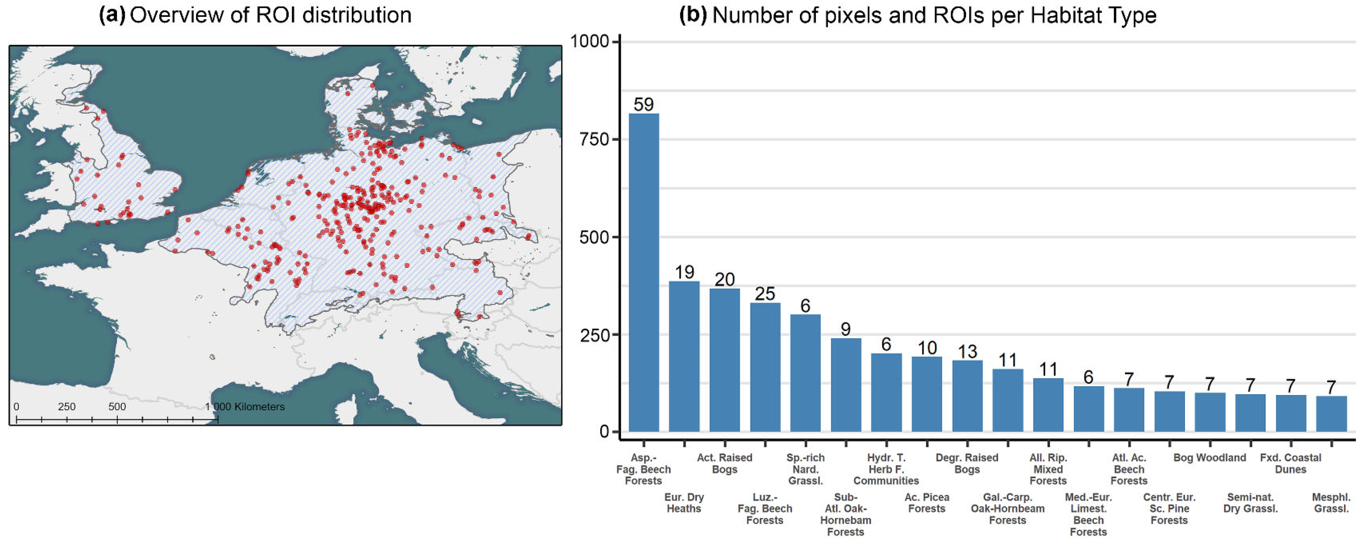
2.1.2. Regions of Interest

An important requirement of supervised remote sensing classification is to generate target spectral signatures for each class that are as representative as possible, particularly if no ground reference data are available. At the same time, we aimed to represent the diversity and variation in the individual habitat types, some of which extend over large geographical areas. Suitable ROIs for classification must therefore meet the requirements of both accuracy and comprehensiveness. This was based, in our case, on the usage of the EEA’s N2000 dataset [16]. This European database contains descriptive and spatial information on all N2000 SACs in the European Union and the habitat types they contain and is generally updated once a year since 2010. In order to avoid an excessive spatial and ecological distance to the actual study area, regions that show high ecological similarities to parts of Germany were screened for suitable areas. For this assessment, we used the climatic stratification of Europe’s environment by Metzger et al. [30], which aggregates Europe into 13 environmental zones based on climatical and ecological similarity. Zones that, while also occurring in Germany, were not separated by zones that did not occur in Germany, were taken into consideration. Suitable SACs were defined by having a coverage rate of at least 75% with only a single terrestrial habitat type and a size of at least 50 hectares. Habitat types that were represented in less than 5 SACs after applying these thresholds were excluded from the survey. That was the case for sub-pannonic steppic grasslands, wooded dunes of the Atlantic and Illyrian Fagus sylvatica forests. We grouped some of the habitat types that share structural similarities and that were at the same time represented by a relatively small number of SACs with little size (see Appendix B,

Table A2. List of habitat type abbreviations. Habitat Types as listed in Annex I of the Habitats Directive are provided with a unique code, which is also referred to here.

Habitat Type	Abbreviation	Habitat Code
Asperulo-Fagetum beech forests	Asp.-Fag. Beech Forests	9130
European Dry Heaths	Eur. Dry Heaths	4030
Active raised bogs	Act. Raised Bogs	7110
Luzulo-Fagetum beech forests	Luz.-Fag. Beech Forests	9110
Species-rich Nardus grasslands, on silicious substrates in (sub)mountain areas	Sp.-rich Nard. Grassl.	6230
Sub-Atlantic oak-hornbeam forests and Tilio-Acerion Forests	Sub-Atl. Oak- Hornebam Forests	9160 + 9180
Hydrophilous tall herb fringe communities	Hydr. T. Herb F. Communities	6430
Acidophilous Picea forests of the montane to alpine levels (Vaccinio-Piceetea)	Ac. Picea Forests	9410
Degraded raised bogs still capable of natural regeneration	Degr. Raised Bogs	7120 + 7140
Galio-Carpinetum oak-hornbeam forests	Gal.-Carp. Oak-Hornbeam Forests	9170
Alluvial Forests and Riparian mixed forests	All. Rip. Mixed Forests	91F0 + 91E0
Medio-European limestone beechforests of the Cephalanthero-Fagion	Med.-Eur. Limest. Beech Forests	9150
Atlantic acidophilous beech forests with Ilex and Taxus in the shrublayer	Atl. Ac. Beech Forests	9120
Central European lichen Scots pine forests	Centr. Eur. Sc. Pine Forests	91T0
Bog woodland	Bog Woodland	91D0
Semi-natural dry grasslands or Molinia Meadows on calcareous substrates	Semi-nat. Dry Grassl.	6210 + 6410
Fixed coastal dunes with herbaceous vegetation (‘grey dunes’)	Fxd. Coastal Dunes	2130
Mesophile Grasslands (Lowland and Mountain Hay Meadows)	Mesphl. Grassl.	6510 + 6520

).

We reduced the size of the ROIs using a negative buffer distance of 150 m. ROI polygons were then converted to raster data with the same cell size as the MODIS reflectance data (500 m). Pixels were assigned to the respective habitat type, if their centre was within the downscaled ROI. This was carried out in order to avoid mixed pixels at the edges of the ROIs as best as possible. We removed ROIs with a minimum size of 5 pixels (corresponding to 1.25 km²) to allow for a sufficient number of homogeneous training pixels per site. Furthermore, we removed pixels that had reflectance values in at least one spectral band outside of the 95th or 5th percentile of all pixels identified as the same habitat type to further reduce mixed pixels.

After reviewing all potential ROIs and applying the chosen thresholds, we obtained between 196 and 221 ROIs, depending on the year, directly representing 18 habitat types and indirectly including an additional 5 habitat types (Appendix B). The total number of ROI pixels ranged between 3846 and 4217 pixels, depending on the year. The distribution of ROI pixels per habitat type differed only slightly between years. On average across all three training years, the most training pixels were available for Asperulo-Fagetum Beech Forests (658 pixels) and European Dry Heaths (422 pixels) (Figure 1). The fewest training pixels were available for Mesophile Grasslands (108 pixels) and Fixed Coastal Dunes (110 pixels). The reflectance spectra of the habitat types compared between all five years and three seasons showed that differences in reflectance between years were generally small and variation in spectra was rather specific for the respective habitat type (see Supplementary Material Figure S1). Slight annual differences in the spring spectra of some habitat types indicate phenological differences at the beginning of the vegetation period. All data analysis was performed in R Version 3.6.0 [31]; spatial calculations were done in ArcGIS Pro 2.7.0 [32].

2.2. Machine Learning Framework

All three machine learning methods used to perform the classification have already been widely used in remote sensing classification and mapping studies [33,34,35,36]. All analyses were performed in R using the packages “randomForest” [37], “C50” [38], and “e1071” [39]. The C5.0 algorithm uses a recursive partition procedure to build decision trees. This is done by splitting the sample based on the predictor variable that provides the most discriminatory power at each internal node. Terminal nodes that do not contribute significantly to the model are removed [35]. Likewise, the RF algorithm is based on decision trees. An ensemble of trees is built from samples drawn with replacement from the training set. Each tree provides a vote selecting the class assignment of a given pixel [40]. In contrast to decision tree classifications, SVMs regard the pixels to be classified as vectors in a multidimensional feature space that results from the number of spectral bands [41]. The goal of the SVM is to fit optimal hyperplanes into the feature space, which act as boundaries between the classes. This is done by maximising the margin between the closest training samples (support vectors) and the hyperplane itself [42].

Table 1. Technical parameters of remote sensing and land cover data used in the classification.

Name	Spatial Resolution	Dates of Acquisition	Spectral Bands	Reference
			Surface Reflectance Band 1 (620–670 nm)
		Years: 2010, 2013, 2014, 2016, 2019	Surface Reflectance Band 2 (841–876 nm)
MODIS/Terra Surface Reflectance 8-Day L3		Recording dates *:	Surface Reflectance Band 3 (459–479 nm)
Global 500 m SIN Grid (MOD09A1 Version 006)	500 Meters	15/04, 23/04, 02/06	Surface Reflectance Band 4 (545–565 nm)	[27]
(Multispectral Reflectance Data)		26/06, 04/07, 20/07	Surface Reflectance Band 5 (1230–1250 nm)
		21/08, 29/08, 06/09	Surface Reflectance Band 6 (1628–1652 nm)
			Surface Reflectance Band 7 (2105–2155 nm)
Corine Land Cover (CLC) 2018, Version 2020_20u	100 Meters	2018	–
(Landuse Data)				[34]

* starting dates of the 8-day composite period.

Table 1. Technical parameters of remote sensing and land cover data used in the classification.

Name	Spatial Resolution	Dates of Acquisition	Spectral Bands	Reference
			Surface Reflectance Band 1 (620–670 nm)
		Years: 2010, 2013, 2014, 2016, 2019	Surface Reflectance Band 2 (841–876 nm)
MODIS/Terra Surface Reflectance 8-Day L3		Recording dates *:	Surface Reflectance Band 3 (459–479 nm)
Global 500 m SIN Grid (MOD09A1 Version 006)	500 Meters	15/04, 23/04, 02/06	Surface Reflectance Band 4 (545–565 nm)	[27]
(Multispectral Reflectance Data)		26/06, 04/07, 20/07	Surface Reflectance Band 5 (1230–1250 nm)
		21/08, 29/08, 06/09	Surface Reflectance Band 6 (1628–1652 nm)
			Surface Reflectance Band 7 (2105–2155 nm)
Corine Land Cover (CLC) 2018, Version 2020_20u	100 Meters	2018	–
(Landuse Data)				[34]

* starting dates of the 8-day composite period.

2.2.1. Parametrisation and Validation

For the parametrisation, all methods had the following approach in common: The ROI pixels of the three years 2013, 2014, and 2016 were divided into training and test sets 30 times each. All training sets consisted of 50% of the ROI pixels and were selected using randomised sampling stratified by habitat type. The test sets consisted of the pixels that were not chosen for the training sets (Figure 2). For each classification method and each pair of training and test sets, the best parameter combination was determined with a grid search and evaluated based on Overall Accuracy (OA) and Kappa. We adjusted RF models using the minimum size of the terminal nodes (nodesize) and the number of trees to grow (ntree) with suitable values for nodesize (1, 2, 3, 4, 5) and ntree (250, 500, 750, 1000, 1500, 2000, 2500). The C5.0 algorithm was adjusted by the smallest number of samples that must be put in at least two splits (minCases) and the trials parameter, an integer that specifies the number of boosting iterations. We tested model performance with various combinations of trials (1, 2, 5, 10, 15, 20, 25, 30, 35, 40, 50) and minCases (1, 2, 3, 4, 5, 6, 7, 8). In regard to SVM, we chose the radial basis function (RBF) as a kernel, which has been widely applied to SVM classification of remote sensing data [41] and is controlled by two hyperparameters γ and C. These parameters define how precisely the hyperplanes are adapted to the classes and control the width of the hyperplane, respectively [43]. We tuned the models using appropriate values of C (0.1, 0.5, 1, 2, 3, 4, 5, 6, 7, 8, 9, 10, 15) and γ (0.005, 0.01, 0.02, 0.03, 0.04, 0.05, 0.06, 0.07, 0.08, 0.09, 0.1, 0.2, 0.5, 1). The parameter combination that provided the best goodness-of-fit measures on average across all 30 test sets was chosen. That resulted in nine models for each of the test years—three based on the different machine learning approaches for each of the three training years. For validation, we built models with the best parameters for each of the three training years using half of their ROI pixels and applied them thirty times to half of the ROI pixels of the two selected validation years (2010 and 2019). To measure the impact of model averaging on predictive performance, the predictions for both test years were averaged by assigning a final class to each pixel based on a majority vote of the nine models.

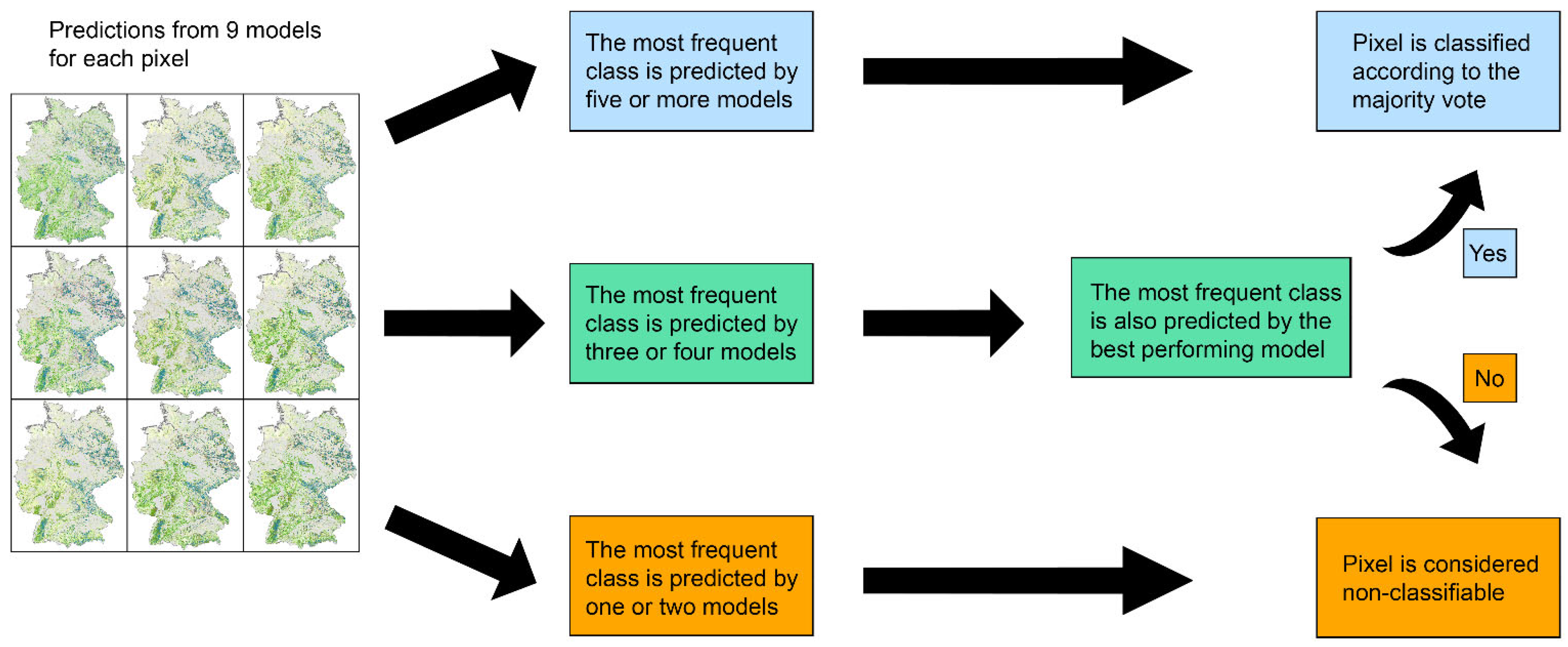
2.2.2. Distance Measure and Model Averaging

Based on all ROI pixels of the respective training year, all nine models were applied to the study area for the years 2010 and 2019 so that nine predictions were assigned to each pixel. Instead of allocating non-classifiable pixels as part of the machine learning algorithms, their assignment was mainly based on the calculation of spectral distance measurements. For pixels that deviated strongly from the average of their class, we assumed the classification to be too insecure and thus labelled these pixels as “non-classifiable.” Distance measurement was conducted by first performing a principal component analysis for all classified pixels. Then, for each pixel, the Euclidean distances between its scores and the respective mean values for all principal components, calculated for all pixels of the respective habitat type, was determined. After standardizing the Euclidean distances of each pixel to zero mean and unit variance, pixels with a Z-score >1 were considered non-classifiable.

In order to make a definitive labelling for all pixels, model averaging was performed for both test years. For each pixel that had not been previously defined as non-classifiable, we determined which class was predicted most frequently in the ensemble approach. If the most frequent class was predicted by at least five models, the majority decision was adopted directly. Pixels with the most frequently assigned class predicted by less than three models were considered non-classifiable. For those pixels whose most frequent class was predicted by three or four models, we adopted the majority decision in case of a match between the most frequently predicted class and the class predicted by the model with the best performance measures. Otherwise, the pixel was considered non-classifiable (Figure 3).

3. Results

3.1. Model Validation

Model validation showed that SVM and RF performed best (SVM: OA 0.721–0.932, Kappa 0.738–0.935; RF: OA 0.724–0.94, Kappa 0.702–0.934) and exceeded the predictive power of C5.0 (OA 0.655–0.932, Kappa 0.668–0.916,

Table 2. Summary of optimal model parameters for each method and training year and the corresponding model performance measures for each validation year.

				2010		2019
Training Year	Method	Best Parameters		Overall Accuracy	Kappa	Overall Accuracy	Kappa
	SVM	γ: 0.09	C: 9	0.778	0.784	0.721	0.738
2013	RF	nodesize: 4	ntrees: 2500	0.801	0.769	0.724	0.702
	C5.0	Trials: 50	MinCases: 5	0.805	0.781	0.655	0.674
	SVM	γ: 0.05	C: 10	0.74	0.757	0.721	0.758
2014	RF	nodesize: 3	ntrees: 2000	0.745	0.731	0.736	0.733
	C5.0	Trials: 30	MinCases: 3	0.689	0.678	0.675	0.668
	SVM	γ: 0.09	C: 15	0.932	0.935	0.78	0.793
2016	RF	nodesize: 5	ntrees: 750	0.94	0.934	0.78	0.747
	C5.0	Trials: 50	MinCases: 8	0.932	0.916	0.716	0.672

). Slightly better results were obtained in each case when the proportions of the respective habitat types were weighted, which has also been adopted for the application of the models. In terms of model performance for validation years, there were distinct differences between training sets, with 2016 models having the highest average predictive power (Kappa 0.809, OA 0.847), followed by 2013 (Kappa 0.741, OA 0.747) and 2014 (Kappa 0.72, OA 0.718). Models built from 2016 training data showed particularly high predictive power for the test year 2010, for which we generally found higher model performance measures than for 2019. We checked for consistency among the training years by having the ROI pixels of individual training years mutually predict each other, which showed performance measures largely comparable to those of the target year applications (OA: 0.658–0.831, see Appendix D). Averaging the model predictions for validation according to majority voting slightly outperformed the best individual model, with OA values of 94.23% for 2010 and 80.34% for 2019.

All models were applied to the two validation years with the determined optimal parameters. Applying the distance measure, between 11.11% (C5.0, 2016) and 13.75% (SVM, 2016) of the total pixels were considered non-classifiable for the target year 2019. The number of non-classifiable pixels differed only slightly between the training years, but it was higher for SVM models with an average of 13.68% than for the other two methods (RF 11.46%, C5.0 11.53%). The same applied to the target year 2010, where slightly more pixels, ranging from 11.29% (C5.0, 2013) to 14.87% (SVM, 2016), were non-classifiable, with the rate for SVM also being higher than for the other two methods (RF 11.94%, C5.0 12.19%) at an average of 14.44%. Overall, the number of pixels for which five or more models predicted the same habitat type was 64.47% for 2019 and 71.0% for 2010. For these pixels, the majority decision was directly accepted as the final classification. The number of pixels for which the most frequent prediction was made by fewer than three models was 1.2% for 2019 and 1.59% for 2010. These pixels were directly declared non-classifiable. For the majority of the remaining pixels (chosen from a maximum of three or four models), the prediction of the majority decision was not the same as the prediction of the model with the best performance. These pixels were also considered non-classifiable. After applying model averaging, the percentage of pixels for which a final classification was available was 64.05% for 2019 and 70.07% for 2010 (Figure 4).

The accuracy measurements of the individual habitat types are reported in

Table 3. Accuracy assessment (user’s accuracy, producer’s accuracy, and F1-score) of individual habitat types for both independent test years 2010 and 2019 for the ensemble prediction from all nine classification models for each year. CI columns show the associated 95% binomial proportion confidence intervals (Clopper-Pearson).

Habitat Type	User’s Accuracy				Producer’s Accuracy				F1-Score
	2010	CI	2019	CI	2010	CI	2019	CI	2010	2019
European Dry Heaths	1.000	0.989–1.000	0.984	0.964–0.995	0.945	0.916–0.966	0.805	0.762–0.843	0.972	0.885
Active raised bogs	1.000	0.990–1.000	0.954	0.928–0.972	0.958	0.933–0.975	0.935	0.906–0.957	0.978	0.944
Degraded raised bogs still capable of natural regeneration	0.847	0.782–0.898	0.620	0.537–0.698	0.986	0.949–0.998	0.802	0.717–0.870	0.911	0.699
Alluvial Forests and Riparian mixed forests	0.826	0.752–0.885	0.574	0.475–0.669	0.983	0.939–0.998	0.344	0.275–0.419	0.898	0.431
Luzulo-Fagetum beech forests	0.997	0.983–1.000	0.856	0.817–0.890	0.723	0.680–0.764	0.551	0.509–0.591	0.838	0.670
Sub-Atlantic oak-hornbeam forests and Tilio-Acerion Forests	0.961	0.921–0.984	0.615	0.556–0.672	0.905	0.854–0.943	0.696	0.635–0.752	0.932	0.653
Semi-natural dry grasslands or Molinia Meadows on calcareous substrates	0.940	0.867–0.980	0.806	0.686–0.896	1.000	0.954–1.000	0.893	0.781–0.960	0.969	0.847
Bog woodland	1.000	0.958–1.000	0.892	0.791–0.956	0.989	0.938–1.000	1.000	0.938–1.000	0.994	0.943
Mesophile Grasslands (Lowland and Mountain Hay Meadows)	0.892	0.804–0.949	0.978	0.885–0.999	1.000	0.951–1.000	1.000	0.921–1.000	0.943	0.989
Fixed coastal dunes with herbaceous vegetation (‘grey dunes’)	0.962	0.893–0.992	0.933	0.838–0.982	0.987	0.930–1.000	0.982	0.906–1.000	0.974	0.957
Asperulo-Fagetum beech forests	0.915	0.894–0.933	0.729	0.703–0.754	0.967	0.953–0.978	0.813	0.789–0.836	0.940	0.769
Galio-Carpinetum oak-hornbeam forests	0.627	0.550–0.700	0.458	0.377–0.540	0.991	0.949–1.000	0.805	0.706–0.882	0.768	0.583
Central European lichen Scots pine forests	0.989	0.938–1.000	0.986	0.926–1.000	1.000	0.958–1.000	0.947	0.871–0.985	0.994	0.966
Atlantic acidophilous beech forests with Ilex and Taxus in the shrublayer	0.909	0.839–0.956	0.473	0.367–0.580	1.000	0.964–1.000	0.977	0.880–0.999	0.952	0.637
Acidophilous Picea forests of the montane to alpine levels (Vaccinio-Piceetea)	0.995	0.970–1.000	0.977	0.941–0.994	0.995	0.970–1.000	0.971	0.933–0.990	0.995	0.974
Medio–European limestone beechforests of the Cephalanthero-Fagion	0.981	0.932–0.998	0.708	0.602–0.799	1.000	0.964–1.000	1.000	0.943–1.000	0.990	0.829
Species-rich Nardus grasslands on silicious substrates in (sub)mountain areas	1.000	0.988–1.000	0.937	0.906–0.960	0.993	0.976–0.999	0.997	0.983–1.000	0.997	0.966
Hydrophilous tall herb fringe communities	0.986	0.959–0.997	0.989	0.961–0.999	0.949	0.911–0.974	0.968	0.931–0.988	0.967	0.978

(user’s accuracy, producer’s accuracy, and F1-score). In overall terms, good to very good classification results were recorded for most classes in the validation process with weighted averaged F1-scores of 0.95 for 2010 and 0.848 for 2019. However, there were some significant differences in terms of accuracy measures between individual classes in 2019, with Galio-Carpinetum oak-hornbeam forests (F1-score 0.583) and Alluvial forests and riparian mixed forests (F1-score 0.431) being the least accurate. Both classes sometimes get misclassified as Asperulo-fagetum beech forest; Alluvial forests are also occasionally mistaken for Sub-Atlantic oak-hornbeam forests. Furthermore, Luzulo- and Asperulo-Fagetum beech forests are sometimes misclassified with each other. However, a more detailed report of the habitat type-specific classification results in the confusion matrices (Appendix C) shows that most individual classes are only to a small extent confused with other classes.

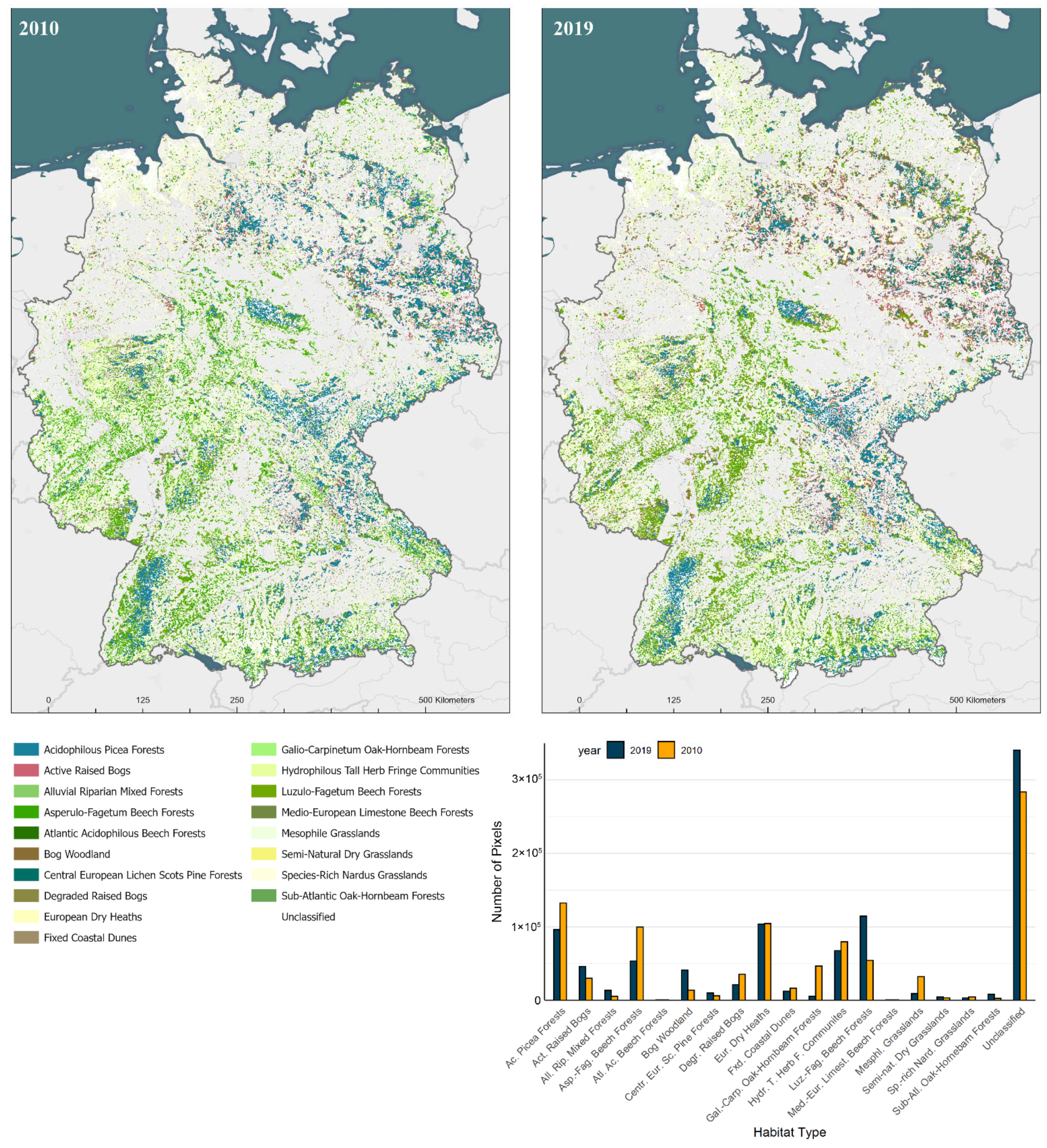
3.2. Habitat Classification

The classification shows the five most common habitat types across both years to be Acidophilous Picea forests, Asperulo-Fagetum Beech forests, Luzolo-Fagetum Beech forests, Hydrophilous tall herb fringe communities, and European Dry Heaths, which together account for 70.62% (2010) and 71.57% (2019) of classified pixels (

Table 4. Changes in the distribution of habitat types in Germany between 2010 and 2019 based on the final ensemble classification results after model averaging. Area of habitat types is given by the number of pixels belonging to a certain class multiplied by the pixel size (500 m²).

Habitat Type	Number of Pixels		Area (km2)		Change (%)
	2019	2010	2019	2010
European Dry Heaths	103,741	104,298	25,935	26,075	−0.53
Active raised bogs	45,864	29,904	11,466	7476	53.37
Degraded raised bogs still capable of natural regeneration	21,085	34,972	5271	8743	−39.71
Alluvial Forests and Riparian mixed forests	13,374	5298	3344	1325	152.43
Luzulo-Fagetum beech forests	114,230	53,938	28,558	13,485	111.78
Sub-Atlantic oak-hornbeam forests and Tilio-Acerion Forests	8017	2243	2004	561	257.42
Semi-natural dry grasslands and Molinia Meadows on calcareous substrates	4600	2910	1150	728	58.08
Bog woodland	40,777	13,455	10,194	3364	203.06
Mesophile Grasslands (Lowland and Mountain Hay Meadows)	8973	32,197	2243	8049	−72.13
Fixed coastal dunes with herbaceous vegetation (‘grey dunes’)	11,884	16,123	2971	4031	−26.29
Asperulo-Fagetum beech forests	53,166	99,378	13,292	24,845	−46.50
Galio-Carpinetum oak-hornbeam forests	5175	46,654	1294	11,664	−88.91
Central European lichen Scots pine forests	9682	6096	2421	1524	58.83
Atlantic acidophilous beech forests with Ilex and Taxus in the shrublayer	150	285	38	71	−47.37
Acidophilous Picea forests of the montane to alpine levels (Vaccinio-Piceetea)	96,253	132,286	24,063	33,072	−27.24
Medio-European limestone beechforests of the Cephalanthero-Fagion	156	386	39	97	−59.59
Species-rich Nardus grasslands, on silicious substrates in (sub)mountain areas	2878	4579	720	1145	−37.15
Hydrophilous tall herb fringe communities	67,282	79,284	16,821	19,821	−15.14
Unclassified	340,712	283,713	85,178	70,928	20.09

). The rarest habitat types are Atlantic acidophilous beech forests (2010: 0.02%, 2019: 0.01%) and Medio-European limestone beech forests (2010: 0.03%, 2019: 0.01%), furthermore, for the year 2010 Sub-atlantic oak-hornbeam forests (0.18%) and for the year 2019 Species-rich Nardus grasslands (0.24%). The average number of ROI pixels per habitat type over all three training years correlates only moderately with the distribution of habitat types in the two target years (Pearson correlation coefficient 2010: 0.56, 2019: 0.51).

A few habitat types are particularly noteworthy in the comparison between 2010 and 2019: The largest decreases in classifiable pixels are found for Galio-Carpinetum forests (−88.9%) and Mesophile grasslands (−72.13%). We saw the highest increase in pixels between 2010 and 2019 in the Sub-Atlantic Oak Hornbeam Forests habitat type with +257% and Bog Woodland with +203%. Considerable differences can also be seen in the quite similar beech forest habitat types (Asperulo-Fagetum & Luzulo-Fagetum Beech Forests). While Luzulo-Fagetum showed a substantial increase of 111.78% in classified pixels, Asperulo-Fagetum showed a decrease of −46.5%. Differences also emerged for conifers: While our results indicated a decline in spruce forests (Acidophilous Picea Forests) between 2010 and 2019 (−27.23%), there was an increase of 58.82% of the Central European lichen Scots pine forest habitat type. For two of the other most common habitat types, only minor differences can be found, namely. for European Dry Heaths (−5.3%) and Hydrophyllous Tall Herb Fringe Communities (−15.13%). Overall, the percentage change of the habitat type cover does not correlate with the number of pixels per habitat type in the ROIs (−0.098) nor with the number of pixels per habitat type predicted by the classification (−0.328). Correlations between the absolute values of the percentage change of each habitat type and its F1-score were also low (−0.23 for 2010 and −0.416 for 2019).

Regarding the spatial distribution of the classified habitat types, besides many similarities in some regions, clear differences were noticeable. The reduction in spruce forests can be recognized directly in the distribution maps, especially in the high altitudes of the Black Forest and in the northeast of the study area, in Brandenburg and Mecklenburg-Western Pomerania. Many of the pixels that are still classified as spruce forest in the Black Forest in 2010 are considered non-classifiable in 2019, which indicates a large-scale dieback of the spruce monocultures found there. In the northeast, on the other hand, a more frequent classification of Bog Woodland is noticeable, indicating a decreasing dominance of spruce in the mixed woodlands there with frequently moist to wet, peaty substrate (Figure 5).

The increasing prevalence of Luzulo-Fagetum Beech Forests can be observed mainly in the low mountain ranges of southwestern central Germany. The spread in these areas is partly at the expense of spruce forests and Galio-Carpinetum forests. Asperulo-Fagetum Beech forests are classified less frequently than Luzulo-Fagetum in 2019, with similar distribution regions mainly in near-natural larger forest areas. However, if both classes of mixed beech forest were added together, this would result in a marginal spread of only 9.1%. An increase in European lichen scots pine forest and Bog woodland, both of which are mainly found in the north-east, in the forest areas of Brandenburg and Mecklenburg-Western Pomerania, is mainly regionally limited to existing occurrences.

Across both years, non-classifiable pixels are mainly found in the north and north-west of Germany, which are strongly characterised by grasslands. A comparison between the years shows that those clusters of non-classifiable pixels are spatially intermixed with semi-natural grasslands, mainly Tall Herb Fringe Communities and Mesophile Grasslands. The same applies partly to European Dry Heaths, which, however, can primarily be located in the forest-free areas of the low mountain ranges.

Regarding raised bogs and fens, an increase in pixels classified as Active Raised Bogs (53.37%) and a decrease in Degraded Raised Bogs (−39.7%) can be observed—both habitat types are mainly found in the heath and moss landscapes of northern Germany and in parts of the low mountain ranges. When both peatland habitats are combined, however, the difference is negligible (3.19% increase).

4. Discussion

Our results show that the models are well able to produce quantitative information on the distribution of individual N2000 habitat types. We found SVM and RF models to provide comparatively high accuracies that are greater than those acquired by the C5.0 models. This is generally in line with the results of similar studies [9,44]. However, in terms of model performance, the differences between individual training years turned out to be larger than those between the individual model types, which makes the use of ensemble methods particularly useful. This could be, for example, due to variation in vegetation status between the years or due to differences in the availability of cloud-free pixels. When designing our models, we explicitly emphasised the applicability in large, heterogeneous study areas and the independence of additional on-site sampling. In this sense, the classification results can be considered successful in regard to the achieved model performance. However, a detailed examination of the results reveals some limitations of the models that are not insignificant for their potential applicability:

The results indicate that the predictive power reaches its limits with habitat types that share close spectral similarities. This can be seen in particular in the strong fluctuations in the cover of individual habitat types, such as in the case of Luzulo- and Asperulo-Fagetum Beech Forests or Active- and Degraded Raised Bogs. We detect significant changes in the spread of these similar habitat types in the comparison between both target years. At the same time, these changes shrink to a much more realistic level as soon as the habitat types are considered jointly on the basis of their similarity. This suggests difficulties in assigning pixels to similar classes due to the low inter-variability in the reflectance properties of these habitat types. On the one hand, this limitation is set by the spectral resolution. At a spatial resolution of 500 m, MODIS data are limited to seven spectral bands, and an accurate assignment between similar habitat types can thus be challenging [10,22]. On the other hand, the use of alternative sensors such as Sentinel-2 would require significantly more computing resources and time due to the size of the study area—and is currently limited to a relatively short observation period from 2015 onwards—but has shown promising results in recent vegetation classification studies [45].

Our methodology is able to provide a good overview with sufficient detail of the distribution of habitat types. The similarity of (semi-)natural areas to the N2000 habitat types studied can be well illustrated. However, depending on the area of application, additional and more precise information may be necessary. Furthermore, we assume that a classification based on our methodology can increase in accuracy in the upcoming years. The reason for this is both the expected increase in the number of SACs and thus the number of potential ROIs, as well as progress in documenting shares of habitat types in already existing SACs. With more data being available in the future, it will be easier to distinguish between individual habitat types that are spectrally similar. We consider the models to be partially able to represent large-scale ecological phenomena. With regard to spruce dieback, local differences and extent of damage can be read from the distribution maps and the reduction in the corresponding habitat type. However, this requires prior knowledge of the distribution of spruce stands and their cultivation methods. The same applies to the assessment of singular, disruptive events, such as storm damage, fire, and flood events. Such events can be identified on the basis of the distribution maps, provided that knowledge of regional impacts is available. This applies, for example, to damage caused by forest fires in the state of Brandenburg 2018 or forest damage caused by windthrow in Lower Saxony in January 2018. The visibility of such events is made possible by the classification criteria of the modelling approach and the designation of non-classifiable areas. A distinction of the causes of habitat reduction cannot be made within the modelling framework; nevertheless, changes due to disruptive weather events can be distinguished from the gradual shift of habitat shares. A regular model application in the sense of change detection would therefore be informative in order to be able to better differentiate between different types of habitat changes.

We regard the methodology of designating non-classifiable pixels to be well suited for this task. There are several indicators for this: One of the clusters of non-classifiable pixels occurring in both years is the grassland-dominated regions of north-west Germany. There is a clear overlap with areas designated as pastures in the Corine land use data. Our models have often regarded these pixels as non-classifiable instead of assigning them to one of the designated grassland habitat types. This indicates the successful delineation of spectral signatures outside and inside the target classes during the supervised classification. Furthermore, fallow areas covered by no or only a little vegetation are also successfully detected as non-classifiable. This can be seen particularly at larger military training areas and in the alpine high-altitude regions. It might be useful to designate additional classes that lie outside the N2000 habitat types (e.g., barren land) and to include pastures in the range of land cover not to be classified.

As expected, it proves difficult to draw clear conclusions about climate influences from gradual changes in the composition of habitat types. This would require a longer observation period, while a backwards-looking application of the models is limited by the data availability of the N2000 SACs. Nevertheless, it is possible to identify trends and compare them with the results of other studies. In a survey of the flora of the Black Forest, Sperle and Bruelheide [46] detected a decrease in vascular plant species characteristic for transition mires and degraded raised bogs, which was associated with climate change effects. While the decline in individual plant species does not yet affect the presence of the habitat type to which they are allocated, this finding is still consistent with trends reflected in our results, also indicating a decline at the habitat level. However, an increase in species associated with wetlands, which was also found, cannot be supported by our results. In a comprehensive study, the European Red Lists of Habitats issued by the European Commission [47] provides a systematic overview of the degree of endangerment of European habitats. Fifteen of the habitat types we studied have a counterpart in the Red List, so we could compare the change in habitat type cover with the vulnerability status of these habitats. Among them, the trend was confirmed for 10 habitat types, which showed a decrease in cover if they were classified as “vulnerable” or “endangered” in the red list and an increase if this was not the case.

5. Conclusions

We introduced a machine learning framework with remote sensing data for habitat monitoring that can evaluate the dynamics of vulnerable habitats on a broad scale. With some limitations, the proposed methodology has been shown to represent the distribution of natural areas comparable to Natura 2000 habitats, which allows the generation of consistent habitat type maps spanning the period of MODIS observations since the early 2000s and well into the future through the use of its follow-up spaceborne sensors, such as VIIRS (Visible Infrared Imaging Radiometer Suite).

Regarding the employed machine learning classifiers, the ensemble approach combining information from SVM, RF, and C5.0 classifications proved to achieve the most accurate habitat assignments while giving valuable information about pixels where clear discrimination based on spectral signatures was not possible. This approach could be further extended with a larger committee of machine learning classifiers, including, e.g., elastic nets, cubist regression trees, or neural networks. The proper classification of smaller habitats or those sharing indistinguishable spectral signatures may also be resolved in the future through the use of high spatial resolution Sentinel-2 data, which would limit the mixing of spectral signatures common in moderate resolution pixels and further allow the incorporation of land surface texture metrics into the classification process.

Although it was impossible to investigate negative impacts on ecosystems within the relatively short time span of the comparison in our study, our results highlight the need for easily applicable habitat monitoring techniques, considering the anticipated challenges in habitat conservation. Enhanced knowledge and understanding about the distribution of habitats is required for environmental managers and decision makers to successfully implement effective conservation measures and to promote ecosystem sustainability. Given that our proposed method can be adapted easily and is carried out with readily available inventory data, we suggest that this method has the potential to be applied more extensively, both temporally and spatially, to monitor habitat distribution from regional to global scales.

References

1. Randin, C.F.; Ashcroft, M.B.; Bolliger, J.; Cavender-Bares, J.; Coops, N.C.; Dullinger, S.; Dirnböck, T.; Eckert, S.; Ellis, E.; Fernández, N.; et al. Monitoring biodiversity in the Anthropocene using remote sensing in species distribution models. Remote Sens. Environ. 2020, 239, 111626. [Google Scholar] [CrossRef]
2. Bittner, T.; Jaeschke, A.; Reineking, B.; Beierkuhnlein, C. Comparing modelling approaches at two levels of biological organisation—Climate change impacts on selected Natura 2000 habitats. J. Veg. Sci. 2011, 22, 699–710. [Google Scholar] [CrossRef]
3. Mahecha, M.D.; Gans, F.; Sippel, S.; Donges, J.F.; Kaminski, T.; Metzger, S.; Migliavacca, M.; Papale, D.; Rammig, A.; Zscheischler, J. Detecting impacts of extreme events with ecological in situ monitoring networks. Biogeosciences 2017, 14, 4255–4277. [Google Scholar] [CrossRef] [Green Version]
4. Pressey, R.L.; Cabeza, M.; Watts, M.E.; Cowling, R.M.; Wilson, K.A. Conservation planning in a changing world. Trends Ecol. Evol. 2007, 22, 583–592. [Google Scholar] [CrossRef] [PubMed]
5. Álvarez-Martínez, J.M.; Jiménez-Alfaro, B.; Barquín, J.; Ondiviela, B.; Recio, M.; Silió-Calzada, A.; Juanes, J.A. Modelling the area of occupancy of habitat types with remote sensing. Methods Ecol. Evol. 2018, 9, 580–593. [Google Scholar] [CrossRef]
6. Vanden Borre, J.; Paelinckx, D.; Mücher, C.A.; Kooistra, L.; Haest, B.; de Blust, G.; Schmidt, A.M. Integrating remote sensing in Natura 2000 habitat monitoring: Prospects on the way forward. J. Nat. Conserv. 2011, 19, 116–125. [Google Scholar] [CrossRef]
7. Roelofsen, H.D.; Kooistra, L.; van Bodegom, P.M.; Verrelst, J.; Krol, J.; Witte, J.-P.M. Mapping a priori defined plant associations using remotely sensed vegetation characteristics. Remote Sens. Environ. 2014, 140, 639–651. [Google Scholar] [CrossRef]
8. Nagendra, H.; Lucas, R.; Honrado, J.P.; Jongman, R.H.G.; Tarantino, C.; Adamo, M.; Mairota, P. Remote sensing for conservation monitoring: Assessing protected areas, habitat extent, habitat condition, species diversity, and threats. Ecol. Indic. 2013, 33, 45–59. [Google Scholar] [CrossRef]
9. Keshtkar, H.; Voigt, W.; Alizadeh, E. Land-cover classification and analysis of change using machine-learning classifiers and multi-temporal remote sensing imagery. Arab. J. Geosci. 2017, 10, 154. [Google Scholar] [CrossRef]
10. Feilhauer, H.; Dahlke, C.; Doktor, D.; Lausch, A.; Schmidtlein, S.; Schulz, G.; Stenzel, S. Mapping the local variability of Natura 2000 habitats with remote sensing. Appl. Veg. Sci. 2014, 17, 765–779. [Google Scholar] [CrossRef]
11. Kopéc, D.; Michalska-Hejduk, D.; Sſawik, ſ.; Berezowski, T.; Borowski, M.; Rosadziſski, S.; Chormaſski, J. Application of multisensoral remote sensing data in the mapping of alkaline fens Natura 2000 habitat. Ecol. Indic. 2016, 70, 196–208. [Google Scholar] [CrossRef]
12. Vanden Borre, J.; Spanhove, T.; Haest, B. Towards a Mature Age of Remote Sensing for Natura 2000 Habitat Conservation: Poor Method Transferability as a Prime Obstacle. In The Roles of Remote Sensing in Nature Conservation: A Practical Guide and Case Studies; Lucas, R., Hurford, C., Díaz-Delgado, R., Eds.; Springer: Cham, Switzerland, 2017; pp. 11–37. ISBN 978-3-319-64332-8. [Google Scholar]
13. Lengyel, S.; Déri, E.; Varga, Z.; Horváth, R.; Tóthmérész, B.; Henry, P.-Y.; Kobler, A.; Kutnar, L.; Babij, V.; Seliškar, A.; et al. Habitat monitoring in Europe: A description of current practices. Biodivers. Conserv 2008, 17, 3327–3339. [Google Scholar] [CrossRef]
14. Corbane, C.; Lang, S.; Pipkins, K.; Alleaume, S.; Deshayes, M.; García Millán, V.E.; Strasser, T.; Vanden Borre, J.; Toon, S.; Michael, F. Remote sensing for mapping natural habitats and their conservation status—New opportunities and challenges. Int. J. Appl. Earth Obs. Geoinf. 2015, 37, 7–16. [Google Scholar] [CrossRef]
15. Council Directive 92/43/EEC of 21 May 1992 on the Conservation of Natural Habitats and of Wild Fauna and Flora. Off. J. Eur. Union 1992, OJ L 206, 7–50.
16. EEA. Natura 2000 Data—The European Network of Protected Sites; European Environmental Agency: Copenhagen, Denmark, 2020. [Google Scholar]
17. Harley, M.; de Soye, Y.; Dickson, B.; Tucker, G.; Keder, G. Biodiversity and climate change in relation to the Natura 2000 network. Adv. Sci. Res. 2009, 3, 35–37. [Google Scholar] [CrossRef]
18. Steinacker, C.; Beierkuhnlein, C.; Jaeschke, A. Assessing the exposure of forest habitat types to projected climate change-Implications for Bavarian protected areas. Ecol. Evol. 2019, 9, 14417–14429. [Google Scholar] [CrossRef]
19. O’Keeffe, J.; Marcinkowski, P.; Utratna, M.; Piniewski, M.; Kardel, I.; Kundzewicz, Z.; Okruszko, T. Modelling Climate Change’s Impact on the Hydrology of Natura 2000 Wetland Habitats in the Vistula and Odra River Basins in Poland. Water 2019, 11, 2191. [Google Scholar] [CrossRef] [Green Version]
20. Sommerfeld, A.; Rammer, W.; Heurich, M.; Hilmers, T.; Müller, J.; Seidl, R. Do bark beetle outbreaks amplify or dampen future bark beetle disturbances in Central Europe? J. Ecol. 2021, 109, 737–749. [Google Scholar] [CrossRef]
21. Bonn, A.; Reed, M.S.; Evans, C.D.; Joosten, H.; Bain, C.; Farmer, J.; Emmer, I.; Couwenberg, J.; Moxey, A.; Artz, R.; et al. Investing in nature: Developing ecosystem service markets for peatland restoration. Ecosyst. Serv. 2014, 9, 54–65. [Google Scholar] [CrossRef] [Green Version]
22. Haest, B.; Vanden Borre, J.; Spanhove, T.; Thoonen, G.; Delalieux, S.; Kooistra, L.; Mücher, C.; Paelinckx, D.; Scheunders, P.; Kempeneers, P. Habitat Mapping and Quality Assessment of NATURA 2000 Heathland Using Airborne Imaging Spectroscopy. Remote Sens. 2017, 9, 266. [Google Scholar] [CrossRef] [Green Version]
23. Marcinkowska-Ochtyra, A.; Gryguc, K.; Ochtyra, A.; Kopeć, D.; Jarocińska, A.; Sławik, Ł. Multitemporal Hyperspectral Data Fusion with Topographic Indices—Improving Classification of Natura 2000 Grassland Habitats. Remote Sens. 2019, 11, 2264. [Google Scholar] [CrossRef] [Green Version]
24. Demarchi, L.; Kania, A.; Ciężkowski, W.; Piórkowski, H.; Oświecimska-Piasko, Z.; Chormański, J. Recursive Feature Elimination and Random Forest Classification of Natura 2000 Grasslands in Lowland River Valleys of Poland Based on Airborne Hyperspectral and LiDAR Data Fusion. Remote Sens. 2020, 12, 1842. [Google Scholar] [CrossRef]
25. Eigenbrod, F.; Gonzalez, P.; Dash, J.; Steyl, I. Vulnerability of ecosystems to climate change moderated by habitat intactness. Glob. Chang. Biol. 2015, 21, 275–286. [Google Scholar] [CrossRef] [PubMed]
26. Pacifici, M.; Foden, W.B.; Visconti, P.; Watson, J.E.M.; Butchart, S.H.M.; Kovacs, K.M.; Scheffers, B.R.; Hole, D.G.; Martin, T.G.; Akçakaya, H.R.; et al. Assessing species vulnerability to climate change. Nat. Clim. Chang. 2015, 5, 215–224. [Google Scholar] [CrossRef]
27. Vermote, E. MOD09A1 MODIS/Terra Surface Reflectance 8-Day L3 Global 500m SIN Grid V006; 2015, distributed by NASA EOSDIS Land Processes DAAC. Available online: https://lpdaac.usgs.gov/products/mod09a1v006/ (accessed on 31 March 2021).
28. Busetto, L.; Ranghetti, L. MODIStsp: An R package for automatic preprocessing of MODIS Land Products time series. Comput. Geosci. 2016, 97, 40–48. [Google Scholar] [CrossRef] [Green Version]
29. EEA. Corine Land Cover (CLC) 2018, Version 2020_20u1. In © European Union Copernicus Land Monitoring Service; European Environmental Agency: Copenhagen, Denmark, 2018; Available online: https://land.copernicus.eu/pan-european/corine-land-cover/clc2018 (accessed on 31 March 2021).
30. Metzger, M.J.; Bunce, R.G.H.; Jongman, R.H.G.; Mücher, C.A.; Watkins, J.W. A climatic stratification of the environment of Europe. Glob. Ecol. Biogeogr. 2005, 14, 549–563. [Google Scholar] [CrossRef]
31. R Core Team. R: A Language and Environment for Statistical Computing; R Foundation for Statistical Computing: Vienna, Austria, 2019. [Google Scholar]
32. Esri Inc. ArcGIS Pro (Version 2.7); Esri Inc.: Redlands, CA, USA, 2021. [Google Scholar]
33. Adam, E.; Mutanga, O.; Odindi, J.; Abdel-Rahman, E.M. Land-use/cover classification in a heterogeneous coastal landscape using RapidEye imagery: Evaluating the performance of random forest and support vector machines classifiers. Int. J. Remote Sens. 2014, 35, 3440–3458. [Google Scholar] [CrossRef]
34. Sun, Z.; Leinenkugel, P.; Guo, H.; Huang, C.; Kuenzer, C. Extracting distribution and expansion of rubber plantations from Landsat imagery using the C5.0 decision tree method. J. Appl. Remote Sens. 2017, 11, 26011. [Google Scholar] [CrossRef] [Green Version]
35. Berhane, T.M.; Lane, C.R.; Wu, Q.; Autrey, B.C.; Anenkhonov, O.A.; Chepinoga, V.V.; Liu, H. Decision-Tree, Rule-Based, and Random Forest Classification of High-Resolution Multispectral Imagery for Wetland Mapping and Inventory. Remote Sens. 2018, 10, 580. [Google Scholar] [CrossRef] [Green Version]
36. Golkarian, A.; Naghibi, S.A.; Kalantar, B.; Pradhan, B. Groundwater potential mapping using C5.0, random forest, and multivariate adaptive regression spline models in GIS. Environ. Monit. Assess. 2018, 190, 149. [Google Scholar] [CrossRef]
37. Liaw, A.; Wiener, M. Classification and regression by randomForest. R News 2002, 2, 18–22. [Google Scholar]
38. Kuhn, M.; Quinlan, R. C50: C5.0 Decision Trees and Rule-Based Models. R Package Version 0.1.3.1. 2020. Available online: https://cran.r-project.org/web/packages/C50/index.html (accessed on 31 March 2021).
39. Meyer, D.; Dimitriadou, E.; Hornik, K.; Weingessel, A.; Leisch, F. e1071: Misc Functions of the Department of Statistics; Probability Theory Group (Formerly: E1071), TU Wien: Vienna, Austria, 2019. [Google Scholar]
40. Pal, M. Random forest classifier for remote sensing classification. Int. J. Remote Sens. 2005, 26, 217–222. [Google Scholar] [CrossRef]
41. Melgani, F.; Bruzzone, L. Classification of hyperspectral remote sensing images with support vector machines. IEEE Trans. Geosci. Remote Sens. 2004, 42, 1778–1790. [Google Scholar] [CrossRef] [Green Version]
42. Mountrakis, G.; Im, J.; Ogole, C. Support vector machines in remote sensing: A review. ISPRS J. Photogramm. Remote Sens. 2011, 66, 247–259. [Google Scholar] [CrossRef]
43. Hastie, T.; Tibshirani, R.; Friedman, J.H. The Elements of Statistical Learning: Data Mining, Inference, and Prediction, 2nd ed.; Springer: New York, NY, USA, 2017; ISBN 978-0-387-84858-7. [Google Scholar]
44. Duro, D.C.; Franklin, S.E.; Dubé, M.G. A comparison of pixel-based and object-based image analysis with selected machine learning algorithms for the classification of agricultural landscapes using SPOT-5 HRG imagery. Remote Sens. Environ. 2012, 118, 259–272. [Google Scholar] [CrossRef]
45. Preidl, S.; Lange, M.; Doktor, D. Introducing APiC for regionalised land cover mapping on the national scale using Sentinel-2A imagery. Remote Sens. Environ. 2020, 240, 111673. [Google Scholar] [CrossRef]
46. Sperle, T.; Bruelheide, H. Climate change aggravates bog species extinctions in the Black Forest (Germany). Divers. Distrib. 2021, 27, 282–295. [Google Scholar] [CrossRef]
47. Janssen, M. European Red List of Habitats—Part 2 Terrestrial and Freshwater Habitats; Publications Office of the European Union: Luxembourg, 2016. [Google Scholar] [CrossRef]
Figure 1. (a) Overview of the distribution of SACs that constitute ROIs in all years. (b) shows the number of pixels per habitat class. The number of ROIs is shown above the bars. A list of all habitat type abbreviations is shown in Appendix B.
Remotesensing 14 00823 g001
Figure 2. Methodology scheme of the classification process. Three machine learning algorithms (SVM, RF, C5.0) are trained and tested using grid search and 30-fold cross-validation on training years 2013, 2014, and 2016 individually and then validated with independent test sets consisting of ROIs from 2010 and 2019. Each model combination (training year and method) is applied to the study area of 2010 and 2019, respectively, resulting in 9 predictive models for each test year. Predictions are averaged by majority vote to generate a final ensemble class assignment.
Remotesensing 14 00823 g002
Figure 3. Methodology scheme for the model averaging process. In the ensemble of nine models, each pixel receives a final classification based on the majority vote of all models. Classes are thus assigned by majority vote if at least five of the nine models predict the same habitat type or if at least three models predict the same habitat type including the overall most accurate individual model. If the classification diverges, i.e., less than three models agree on the predicted habitat type, the pixel is also added to the amount of non-classifiable pixels, in addition to those that were previously excluded due to large spectral distances to the average of their class.
Remotesensing 14 00823 g003
Figure 4. Heatmap of the number of models predicting the most frequent class per pixel. Colour bars show the proportions of pixels whose most frequent classification is made by the corresponding number of models. In both years, five or more models predict the same class for the majority of pixels, thus directly adopting the majority decision of the ensemble. The portion of pixels that are directly defined as non-classifiable is <2% in both years (less than 3 models predicting the most frequent class).
Remotesensing 14 00823 g004
Figure 5. Final results of the habitat classification for Germany in 2010 and 2019. Each pixel was assigned a final prediction based on the ensemble of nine models for each year. The change in the number of pixels per habitat type between 2010 and 2019 is shown at the bottom right.
Remotesensing 14 00823 g005