1. Introduction
Technological progress and development methods of processing spatial data have popularized the use and increased the availability of various products presenting information about the area. Laser scanning became a dynamically developing technology at the turn of the 21st century and is finding an increasing number of applications in various fields of science. Data from an airborne laser scanning system (ALS) significantly facilitate and accelerate the collection of information about the topography and terrain, which leads to both cooperation and competition with the technology and products of classical photogrammetry and geodesy. Currently, the construction of digital terrain models (DTMs) and digital surface models (DSMs) using LiDAR data is common, but the identification of agricultural land boundaries based only on point clouds is a complex issue.
Light detection and ranging (LiDAR) is an active remote sensing system that first generates a laser pulse and then records the energy reflected from a given surface. Knowledge of the time of signal generation and the moment of its reception, as well as the properties of the generated light wave can be used to determine the distance to the object. Airborne laser scanning, which is performed using a flying plane or helicopter, works according to this principle. The system uses two main components: a laser scanner, which collects information about the distance between the scanner and a point on the ground surface, and a combination of Global Positioning System (GPS) and the inertial navigation system (INS), whose task is to measure the position and orientation of the system. As a result, data are acquired in the form of a point cloud [
1].
The point cloud is not the final product. It is a set of data (points), defined by spatial coordinates, with stored information about intensity, RGB color, and echo. This representation reveals a wealth of information, and when processed into numerical models, it enables subsequent applications.
Airborne laser scanning and its products in the form of point clouds and digital terrain models and digital surface models are increasingly used. Precise terrain models contain a large amount of detailed information. Compared to photogrammetry, they enable the study of terrain overshadowed by vegetation. Therefore, this study focuses on the possibility of using LiDAR sensor to identify places of land use changes—agricultural boundaries.
Identification of the course of agricultural boundaries is important to control in the direct agricultural subsidies system (Integrated Administration Control System—IACS) [
2]. The Land Parcel Identification System (LPIS), which is a part of IACS, is a system supporting direct subsidies to farmers, which depend on the area of crops. Farms with a minimum agricultural area of at least 1.0 ha, consisting of agricultural parcels of at least 0.1 ha, qualify for direct payments. The procedure is based on the farmer filling in a declaration, which involves specifying the area of crops intended for payments. The purpose of the control is to determine whether the submitted declaration is correct, i.e., whether the land declared by the farmer is indeed eligible for subsidies. Discrepancies are evidence of irregularities in the declarations, which should be corrected by the farmers. So far control of applications within the framework of direct payments for land is carried out by two methods, i.e., field inspection, most often carried out with the use of GPS technology, and the so-called “photo” method, based mainly on high-resolution satellite images or aerial images.
This study attempts to answer the question of whether ALS data can be used as a basis for inspecting agricultural land boundaries. LiDAR data are a powerful source of spatial information that includes not only coordinates but also intensity, return numbers, and point cloud classification data. Due to the increasing density of acquired data, ALS is increasingly used in new fields.
The purpose and novelty of this study was the attempt to automate the detection of agricultural land edges by using only LiDAR data in the analysis. The innovation of the method is the use of only airborne laser scanning data to indicate the course of agricultural land boundaries. Determination of the agricultural land boundary is important in the process of checking and updating the reference databases of the Land Parcel Identification System. The proposed algorithm—based only on free LiDAR data—was able to detect inconsistencies in farmers’ declarations.
2. Literature Review
The data coming from the LiDAR sensor are characterized by high measurement accuracy. The resulting digital terrain models and digital surface models depict the surrounding reality in detail. These features determine the multidirectional use of airborne laser scanning in various fields of science, such as engineering solutions—calculation 3D displacements of bridges [
3], 3D object detection along the road [
4,
5], building extraction [
6,
7], land cover change detection, and forest succession monitoring [
8,
9] for heterogeneous land use urban mapping [
10], coastal monitoring [
11,
12], or archeological research [
13,
14].
The subject of the LPIS is widely discussed in many publications. Among other things, researchers compare the LPIS to the national cadastre. Reference [
15] evaluated the extent to which the reference data from the cadastral register are modified in the LPIS in Poland. Reference [
16], using the LPIS of the Republic of Ireland, demonstrated significant differences in cropland/grassland reporting between an inter-annual based reporting schema and a land use history approach. Research has also been conducted on a data model for the collaboration between land administration systems and LPIS [
17]. Study [
18] focuses on a conceptual model of a large Turkish rural SDI design that combines the sensor usage and attribute datasets for all types of rural lands. In India, a government program used high-resolution aerial and satellite orthophotomaps, Global Positioning System, and electronic total stations (ETSs) to create and update land cadastres in a short time [
19]. Reference [
20] also analyzes the quality characteristics of orthoimages for visual identification of agricultural fields. Reference [
21] presents a field boundary detection technique based on deep learning and a variety of image features which was combined with the graph-based growing contours (GGCs) method to extract agricultural fields in a study area in Northern Germany.
Airborne laser scanning is increasingly used in research to identify the type of land cover [
22]. Reference [
23] evaluated the use of high-resolution LiDAR for classification of native and tame grasslands and compared these classifications to the best available landcover mapping product that is currently available for this area. Reference [
24] evaluated the effectiveness of integrating LiDAR data with high spatial resolution near-infrared digital imagery for object-based classification of land cover types and dominant tree species, using decision tree analysis. In [
25] the authors proposed a process for objective and automated identification of agricultural parcel features based on processing and combining Sentinel-2 data (to sense different types of irrigation patterns) and LiDAR data (to detect landscape elements). Another example of combination cadastral data and remote sensing is in article [
26] where high-resolution multi-spectral WorldView-2 satellite images were used with the object-oriented approach to image classification and image classification algorithm creation. The main objective is to compare the results obtained with the traditional methods of cadastral land evaluation and the results obtained by the methods of remote sensing. Analyses were performed for an area of Butmir Municipality in Sarajevo. Remote sensing data such as Sentinel-1 radar images were also used for mapping the different crops in the Camargue region in Southern France. In this study, deep machine learning was used to perform land classification [
27]. Reference [
28] proposed a geographic object-based image analysis approach to enable semiautomatic land classification and mapping using LiDAR elevation and intensity data. In [
29], the authors used a hybrid capsule network for land cover classification using multispectral light detection and ranging data. Reference [
30] focused on the extraction of uncultivable trails, ditches, and cultivated field parcels within farmland on the basis of a LIDAR high-resolution gridded DEM. Reference [
31] discussed the impact that the quality of the digital elevation model has on the final result of landslide susceptibility modeling. The landslide map was developed on the basis of the analysis of archival geological maps and the light detection and ranging digital elevation model.
3. Specification of Test Data
The test area is located in Lubelskie Voivodeship in the village of Zimno and includes only the agricultural lands on which this study focuses. The test area was characterized by varied terrain. The laser data used in the study were taken from the ISOK project [
32]. ISOK is a Polish information security system created with the aim of improving the protection of the economy, environment, and society against extraordinary threats, in the first place against floods. The basic specifications of the ISOK project are: 12 points per square meter, average distance between the points is 0.3 m, overlap between scans ≥20%, scan cross angle ≤±25°, min scan lane width ≥100 m, and laser beam diameter ≤0.5 m. The obtained data are in the PL-1992 situation system and PL-KRON86-NH elevation system, with additional information, i.e., intensity and min 4 echo. In the study area, in accordance with the Regulation of the Minister of Regional Development and Construction on land and building cadastres [
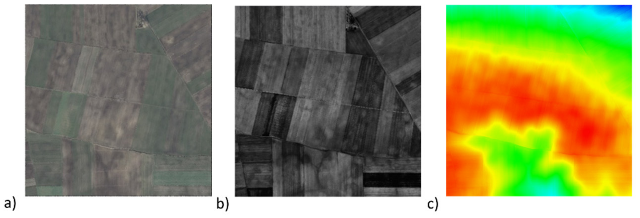
33], the following agricultural land was distinguished: arable crop land, marked with the symbol R; permanent grassland, marked by the symbol Ł; and permanent pastures, marked with the symbol Ps. In the selected area, the agricultural land should correspond to the cadastral parcels. This would make it possible to check whether there is any anomalous information in the area, indicating a discrepancy between the declarations in the payment system. Two study samples were selected for analysis in order to determine the actual land use status. A visualization of the area is shown in
Figure 1.
4. Scheme of the Proposed Algorithm
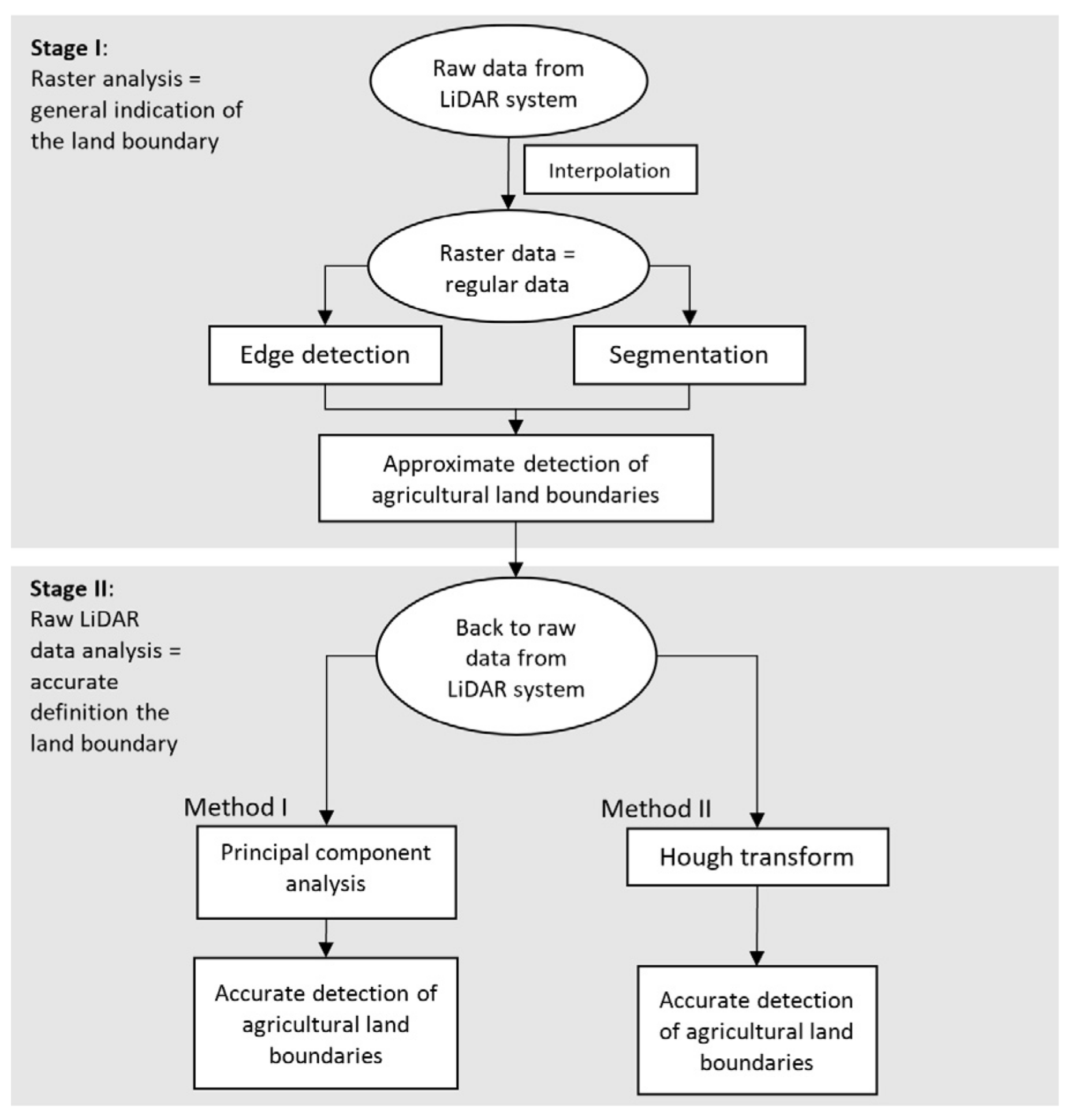
The proposed algorithm consists of two stages. In the first stage, a point cloud is interpolated into a regular grid with a resolution of 0.3 m. Nearest neighbor interpolation was used. Two algorithms are used with the obtained rasters: edge detection and segmentation, on the basis of which the approximate location of agricultural land boundaries is estimated. In the next stage, we returned to the raw point cloud for pre-selected areas from the first part. Two methods were used for the original data: PCA and Hough Transform, which allowed for precise determination of agricultural land boundaries. The scheme of the algorithm is shown in
Figure 2.
5. Detection of Agricultural Land Boundaries from Raster Data
As a first step, an initial detection of agricultural land was undertaken using a point cloud stored as a raster. For this purpose, rasters with a resolution of 0.3 m were generated—images of intensity, classification, height differences, and RGB values.
An edge detection and segmentation process were performed in the MATLAB environment.
5.1. Edge Detection
Edge detection was carried out using the combined operators of Prewitt and Canny [
34], based on intensity and classification rasters. It was decided to combine the two methods in order to obtain a more reliable agricultural land boundary. The Prewitt operator, based on gradients, more accurately determined the edges, but the information about them was point-wise. The Canny operator, on the other hand, introduced linear information but detected undesirable ploughing traces in the fields. Ploughing traces were recorded as lines, which made it difficult to eliminate them in subsequent steps. In the next step, simple morphological operators (erosion and dilation) were applied to remove noise in the image. The performed work made it possible to eliminate many errors and better illustrate land use boundaries in the analyzed area. However, errors are still visible. The result of this stage is presented in
Figure 3.
5.2. Segmentation
Segmentation was used as a further supporting step. The aim was to roughly determine the areas of individual agricultural lands. Segmentation was carried out on the intensity image.
It was decided to use the multi-resolution algorithm (MRS). This is one of the most widely used segmentation models. It is based on the minimalization of the average heterogeneity in a single object extracted from an image [
35]. This algorithm was chosen because a literature review suggested that this segmentation method would be more accurate [
36,
37].
The first key parameter of the algorithm is scale, i.e., the size of objects (segments) in the analyzed area. In this study, the value of 200 is used. In addition to the scale parameter, two additional parameters are required: shape and compactness [
38]. The best results were obtained for values of 0.9 and 0.1, respectively. The segmentation result is shown in
Figure 4.
The performed work allowed for a preliminary identification of the areas of agricultural fields, as well as their boundaries. The effect of the work is illustrated in
Figure 5.
As can be seen from
Figure 5, noise—incorrect edges in object detection—is still present. The integration of edges and segments can be used to identify some of them. Incorrect edges, related to ploughing traces in the fields, were located by correct segments in this area—this mainly concerns three parcels in the central-western part of the study and one parcel in the south-eastern part. Furthermore, in a few parts the segmentation did not work properly. This was due to the similarity of intensities in the neighboring parcels (see
Figure 1b). The different edges in these areas indicate the locations of possible errors (mainly the central and central-southern part of the study). The stage described in this subsection is considered as a prelude to further work aimed at more accurate identification of agricultural land boundaries.
6. Accurate Detection of Agricultural Land Boundaries
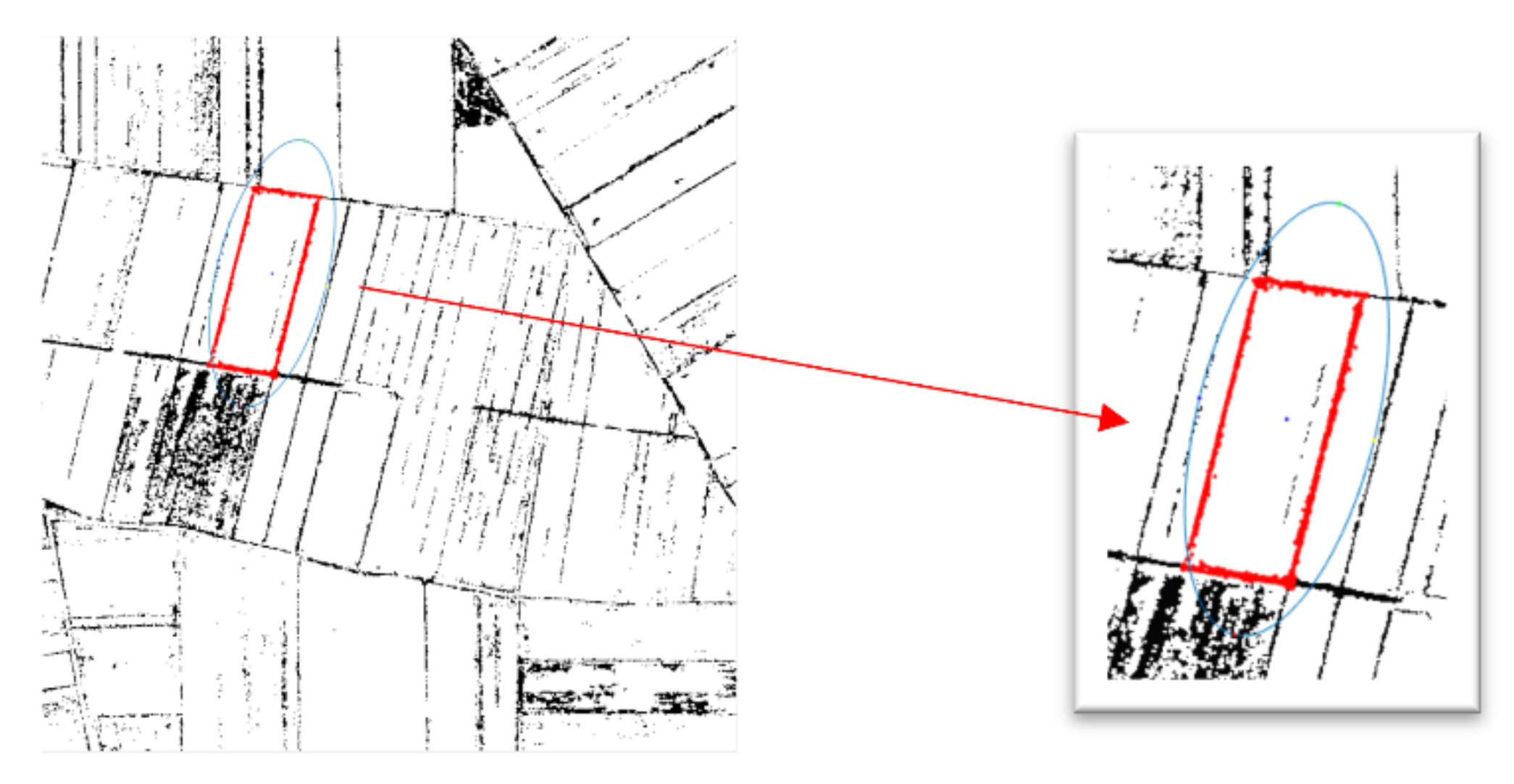
After identification of initial regions of agricultural land boundaries, there was a return to the original point cloud, but this was limited to the indicated sub-areas defining the course of agricultural land boundaries. It was decided to return to distributed data because there are several airborne laser scanning points per image pixel, which will significantly increase the accuracy of the edge location (
Figure 6). Therefore, the original data increase the amount of information that can define the agricultural land with higher accuracy.
In this study, precise detection of agricultural boundaries was presented for two test areas (segments). In the first area, the segment boundaries coincided entirely with a single area of agricultural land. In contrast, the second selected segment included additional agricultural boundaries within its area. Therefore, two approaches for precise identification of agricultural boundaries with the use of scattered data (irregular point cloud) were applied in this study. In the first one, a solution based on principal component analysis was used to determine land parcel boundaries. On the other hand, the second approach used Hough Transform.
6.1. Boundary Detection Using Principal Component Analysis—Test Area No. 1
The first test field is an area of agricultural use whose extent overlaps with the rough edges delineated in stage 1 (
Figure 7).
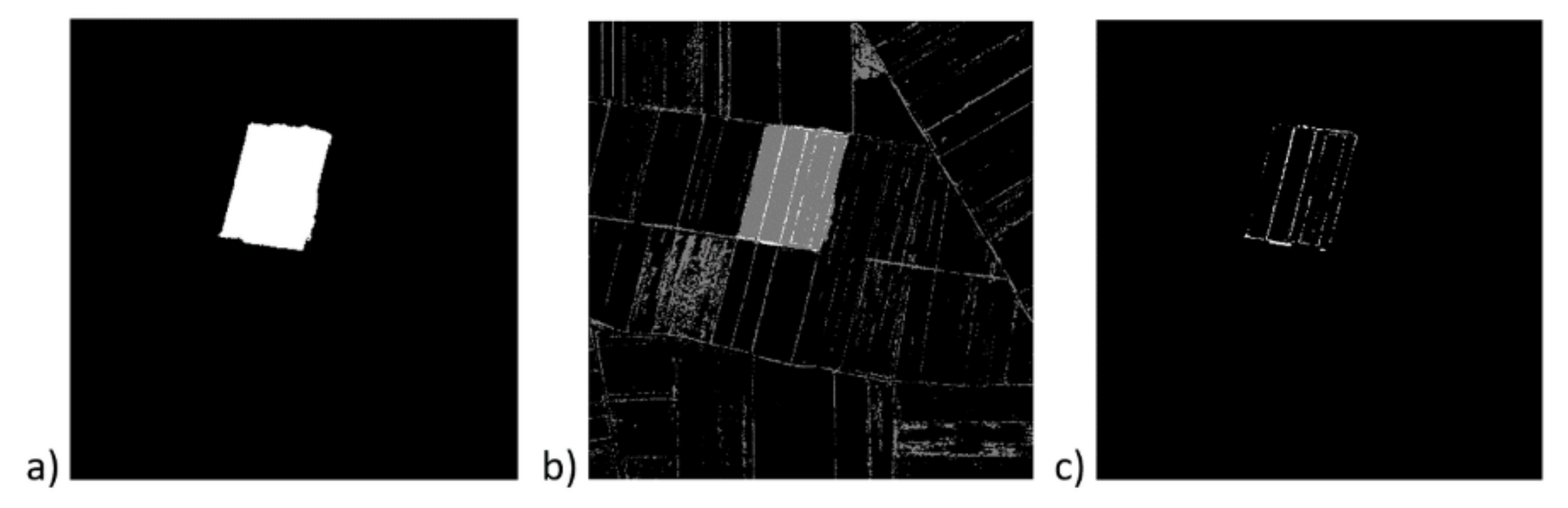
Analyses began by indicating the test area (segment) from the segmentation image (
Figure 8a), then a product was performed with the raster depicting the edges of the agricultural (
Figure 8b), resulting in an image showing only the edges of the segment (
Figure 8c).
The next stage leading to a correct determination of the edges was grouping the set of points into four parts containing points describing each parcel edge separately. For this purpose, a solution based on principal component analysis (PCA) was used. This solution allows us to determine the scatter model of the dataset in the form of a probability ellipse. Each pixel in the image is defined by two variables, the X variable and the Y variable (column number, row number). The ellipse is plotted based on the assumption that the given two variables follow a two-dimensional normal distribution (Gaussian distribution). The orientation of ellipse depends on the sign of correlation coefficient between variables, the size of the ellipse is determined by the intervals and its center is defined by the averages of the variables X and Y. The term intervals refers to the root of the eigenvalues multiplied by the user-selected value. Eigenvalues can be interpreted as proportions of the variance explained by correlations between relevant variables. Therefore, in solving this task, the values of variance and covariance were calculated for the variables X and Y to build the designated perimeter of the object.
The value of variance, which determines the diversity of the community, is equal to the sum of the arithmetic mean of squares of deviations of individual feature values from the arithmetic mean of the community. The unconstrained variance estimator for
X and
Y coordinates was calculated from the following formulas [
39]:
—the variance for X/Y calculated from the sample—unbiased variance estimator;
cov(X,Y)—covariance of a variables X, Y set;
x/y—sample mean value for X/Y;
/—value of the X/Y variable for the i-th point
n—sample size.
The covariance value, which determines the linear relationship between the random variables
X and
Y, can be calculated from the following formula:
As a result of the calculations performed, the variance–covariance matrix can be constructed for X, Y coordinates. From the obtained matrix, the eigenvalues of the matrix can be calculated.
The obtained variance–covariance matrix and eigenvalues were used to calculate the ellipse parameters, i.e., orientation and size of the ellipse according to Hausbrandt’s formulas [
40].
Ω—the omega angle between the horizontal line and the direction of the eigenvector with the larger eigenvalue;
—the variance for X/Y calculated from the sample—unbiased variance estimator;
cov(X,Y)—covariance of a variables X, Y set.
The lengths of the minor (a) and major (b) half-axes of the confidence area ellipse were calculated from the formulas below:
e1—the length value for the minor half-axis of the ellipse;
e2—the length value for the major half-axis of the ellipse;
a1—minor eigenvalue of the test area object;
a2—major eigenvalue of the test area object.
In the above formula, the square root of the eigenvalues was multiplied by 2, which means that 95.5% of the feature values lie at a distance ≤2 from the expected value. The center of gravity was calculated as the arithmetic mean of the
X,
Y coordinates, which determined the midpoint of the ellipse. The obtained parameters can be used to determine the span of the probability ellipse and to determine the main directions along which the points defining the boundaries of the parcel are arranged (
Figure 9).
The parameters of the ellipse also made it possible to divide the points into four sets of data that define four corresponding boundaries. In each of the four sets of points, a simple least squares approximation was performed (
Figure 10). The approximation is an iterative process that, in successive iterations, discards outlier points from the straight line until the agricultural edges are accurately determined. Outlier points are those points that lie further than the average distance of the points from the straight line obtained in successive iterations. The iterative process ends when the sum of the squares of the outliers reaches a minimum.
The intersections of the detected lines determined the vertices of the sought parcel.
6.2. Boundary Detection Using Hough Transform—Test Area No. 2
The second test field was an erroneously delineated segment. The rough edges produced in the first stage indicate that there is probably more agricultural land here (
Figure 11).
Similar to test area no. 1, a segment was first selected on which a raster representing the edges of the utilities was overlaid, resulting in a binary image containing only the edges of the segment (
Figure 12a–c).
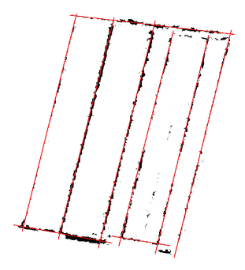
The selected segment contains not only edges describing its perimeter but also several edges inside the area. The study showed that the principal components method cannot automatically write to separate sets of points representing each edge (those inside and outside). Therefore, Hough Transform was used to select and identify all the edges of the analyzed area. Hough Transform enables fast detection of straights in a binary image [
41]. When detecting collinear pixels in an image in this method, it is possible to indicate the number of straights that need to be detected. In this study, nine lines were detected (
Figure 13).
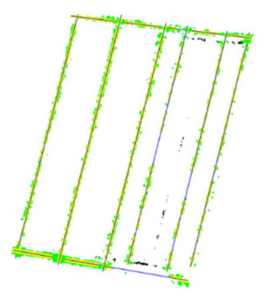
Based on the detected lines, it was possible to group the scattered points into appropriate sets, defining the course of the edge. The condition determining points belonging to a given edge was the distance of the point from the straight line. Thus, nine sets of points were defined, and in each set a straight line was approximated by the least squares method (
Figure 14).
In the next step, the vertices of the areas where the lines intersect were determined. Next, the vector cadastral data were overlaid on the raster representing the edges of the agricultural land (
Figure 15). According to IACS, there can be several types of agricultural land in each parcel of land. However, after visual verification it was found that in the third segment there is one agricultural area of land in the whole cadastral parcel. Therefore, the inclusion of two straights in further analyses was discontinued. The straights are indicated by arrows in
Figure 15.
7. Analysis and Discussion of the Obtained Results
7.1. Test Area No. 1
Test area no. 1 was the arable crop land (R) corresponding to cadastral parcel no. 700. The analysis of the obtained results consisted of comparing the borders of the agricultural land obtained by means of the PCA (
Section 6.1) with the borders of the agricultural land from the cadastral records. For this purpose, additional points were inserted on both lines at corresponding intervals of 0.5 m. Next, deviations were determined as distances between corresponding points.
Western boundary (W): Conformity of agricultural land boundaries with the data recorded in the land cadastre was observed. Obtained deviations are within the range from 0.23 to 0.35 m. The average value is 0.29 m.
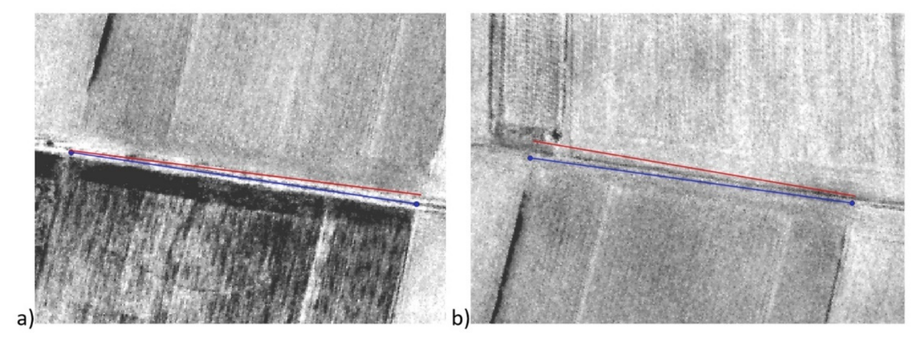
Southern boundary (S): Much larger differences are obtained. Deviations range from 0.37 to 2.16 m, with an average value of 1.26 m. Anomalous information is observed, showing a discrepancy between the declaration and the actual state of use (
Figure 16a). There is a road running in the area, and its boundary is not clear, resulting in changes in the actual state of use for these parts of the parcel.
Eastern boundary (E): Conformity of agricultural land boundaries with the data recorded in the land cadastre was observed. Deviations range from 0.13 to 0.39 m. The average value is 0.26 m.
Northern boundary (N): The largest differences were obtained for the northern boundary of the agricultural land (
Figure 16b). LiDAR determined a completely different course of the agricultural land boundary than indicated by the land cadastre. Deviations range from 1.81 to 4.21 m. The average value of deviations is as high as 3.01 m. Analyzing the data against the intensity map, it can be observed that both the LiDAR data and the cadastre data show discrepancies in relation to the actual land use.
The analysis is presented in two tables.
Table 1 gives the summarized results for the analyzed agricultural land.
It is noted that the largest amount of anomalous information occurs for areas of agricultural land boundaries with field roads.
Table 2 is a comparison carried out for two variants: The first considers the situation of the agricultural land–agricultural land boundary and the second the agricultural land–field road.
7.2. Test Area No. 2
After the analysis of the cadastral data, it was revealed that the selected segment consists of three agricultural lands—R, Ł, corresponding to cadastral parcels with the numbers: 702 (R), 705 (R), and 707 (Ł). The algorithm based on Hough Transform correctly extracted these three areas.
As a first step, a detailed analysis of the agricultural land R for parcel 702 was carried out. Western boundary (W): Conformity of agricultural land boundaries with the data recorded in the land cadastre was observed. Deviations range from 0.23 to 0.40 m. The average value is 0.31 m.
Southern boundary (S): Much larger differences were obtained. The deviations range from 1 to 1.61 m, with an average deviation of 1.31 m. In this area we are dealing with a field road, the course of which is unclear. A discrepancy between the declaration and the actual state of use can be seen in the form of a systematic shift between the LiDAR data and the agricultural land from the land cadastre (
Figure 17a).
Eastern boundary (S): For the eastern boundary, deviations of 0.40–0.70 m were obtained, with a mean value of 0.55 m.
Northern boundary (N): Much larger differences were obtained (
Figure 17b). The deviations range from 0.66 to 1.96 m, and the mean value of the deviations is 1.15 m. In this case a field road is also located in the area.
Due to the repeated spatial situation, the results for parcels 705 and 707 are grouped together in
Table 3. For both parcels similar types of differences to parcel 702 appeared, as discussed above. The results for plot 702 are also included in the table.
A similar rule was observed as in the previous analyses, i.e., a much higher agreement of boundaries for the land–land boundary variant than for the land–field road boundary variant. This is presented in
Table 4.
8. Conclusions
In summary, the proposed algorithms make it possible to carry out controls in the system of direct payments to agriculture. The use of laser data makes it possible to determine specific agricultural land and to determine the size of anomalous information. Correctness has been noted in relation to the conformity of the actual statue with the declaration in the case of boundaries of adjacent agricultural land (variant 1: land—land). However, in areas where there are borders of agricultural land with field roads, there are visible discrepancies (variant 2: land—field road). In these areas, anomalous information connected with the difference between the actual use of a given area and the legal status recorded in the declaration should be noted.
The obtained results were considered satisfactory. LiDAR proved to be very useful technology in the process of detecting agricultural boundaries. Most of the boundaries were readable in the laser data.
The advantage of using a point cloud over traditional aerial images is that an additional elevation information can be used. In the case of aerial images, analyses are carried out on 2D data stored as a raster. In the developed algorithm, the second step returns to the raw point cloud. The knowledge of an additional Z coordinate may allow for more precise edge detection in areas where the 2D information is ambiguous.
It was noted that the introduction of higher resolution data would certainly contribute to an increase in accuracy. The use of laser data from a UAV flight would allow a more precise determination of boundaries in doubtful cases, not fully legible in the case of the data used in this study (average distance between points 0.3 m).
The two-stage approach to analysis also proved to be a valuable solution. Edge detection and segmentation algorithms used in the first stage allowed us to roughly estimate the area and boundaries of individual agricultural lands. In the second stage, we returned to the original data for the locations presenting the contours of the agriculture boundaries. In the developed method of detecting straights, two approaches were used. Two approaches were chosen because the first area is a rectangular parcel of land and the second test area is a rectangle with an internal land boundary, and precise determination of the land boundary is possible if only one boundary is displayed in the raster image. Therefore, in each approach, the aim was to divide the point cloud into datasets representing only one land use boundary. With such datasets it is possible to approximate straights with higher accuracy than by using raster data. Detected land use boundaries are described by the equation of the straight line, determined in an iterative process, wherein subsequent iterations’ outliers are rejected. Thus, the obtained straight line reliably reflects the course of land use boundaries detected based on ALS data.
The created algorithm allowed the detection of inconsistencies in farmers’ declarations. These were related to areas of field roads that were incorrectly declared by farmers as donated land, when in fact they should be excluded from subsidies. It was detected that both test areas, test field 1, areas belonging to field roads with an average width of 1.26 and 3.01 m, and test field 2, areas belonging to field roads with an average width of 1.31, 1.15, 1.88, and 2.36 m, were incorrectly classified by farmers as donated land.
In this study the authors focus on identification of land boundaries between land uses covered with low vegetation. In the next research, the authors intend to analyze the boundaries of parcels that are farmed and covered with different species of plants. Such diversity can help at the stage of segmentation because each species can have a different intensity value. Different intensity value will contribute to easier initial identification of parcel edges. At the stage of precise identification of plot boundaries, on the other hand, it may be necessary to select only points reflected from the ground. Then it will be necessary to perform a filtering of the lidar data to be used for further analysis.
In conclusion, the method used in this study based on LiDAR data is useful for automatic verification and monitoring of anomalous information showing inconsistency of the declaration with the actual state of land use.


