
A Novel Method for Hyperspectral Mineral Mapping Based on Clustering-Matching and Nonnegative Matrix Factorization


Abstract
:1. Introduction
2. Materials
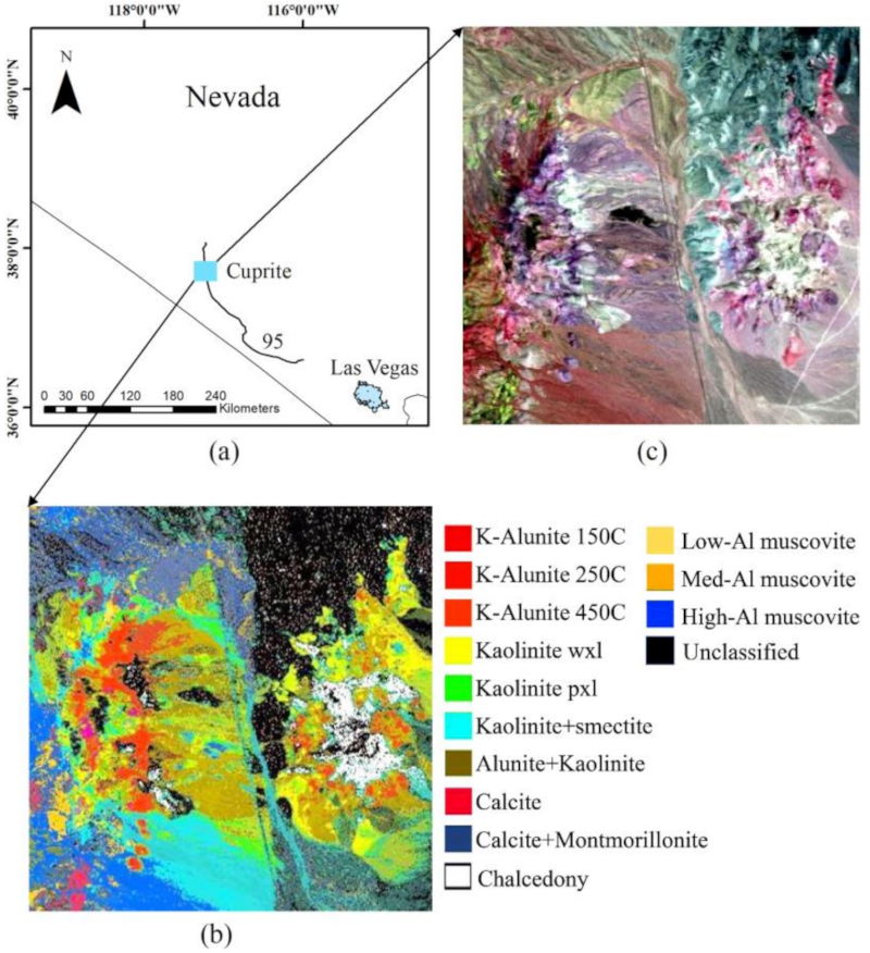
2.1. Study Area
2.2. Datasets
2.2.1. Hyperspectral Data
2.2.2. Spectral Library
3. Methodology
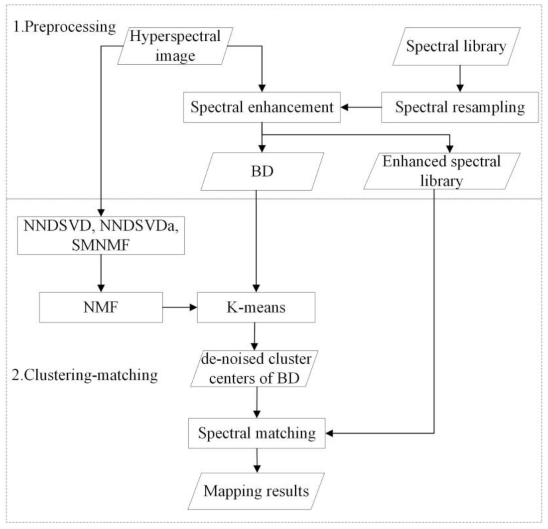
3.1. Spectral Preprocessing
3.2. Clustering-Matching
3.2.1. Feature Extraction
3.2.2. Clustering
3.2.3. Matching
3.2.4. Accuracy Assessment
4. Results
5. Discussion
6. Conclusions
- In feature extraction, the proposed NMF initialization method based on SM performs better than the widely used matrix factorization initialization method in mapping accuracy and efficiency.
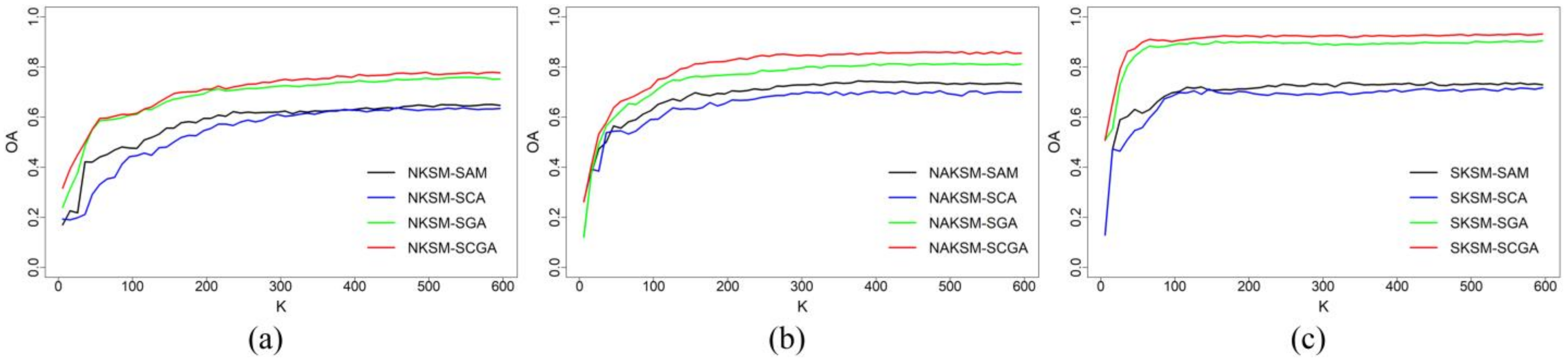
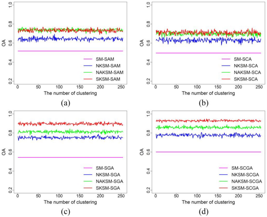
- For k-means clustering, setting K to the spectral curve number of a mineral spectral library or larger can effectively improve the mineral mapping accuracy of clustering-matching.
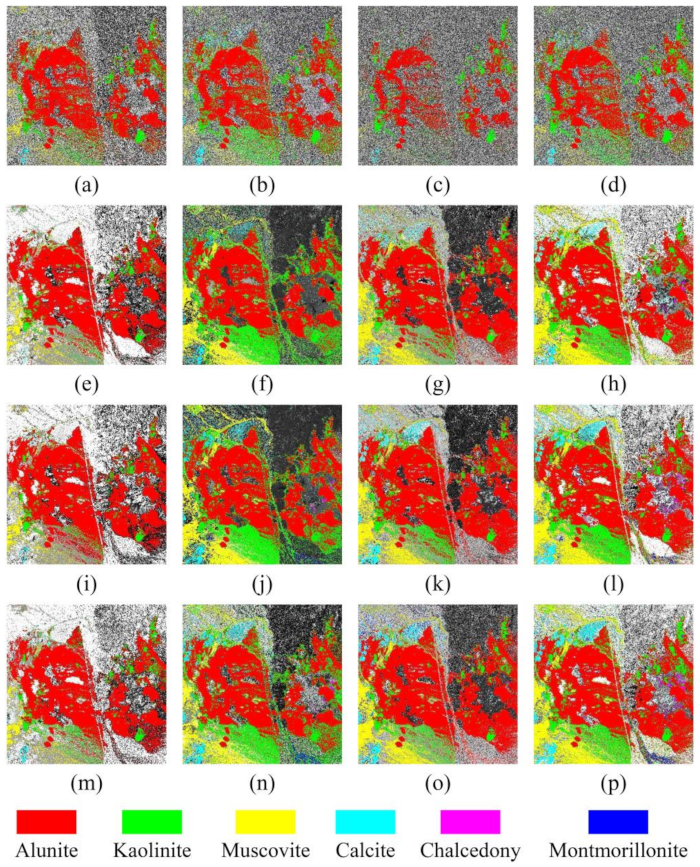
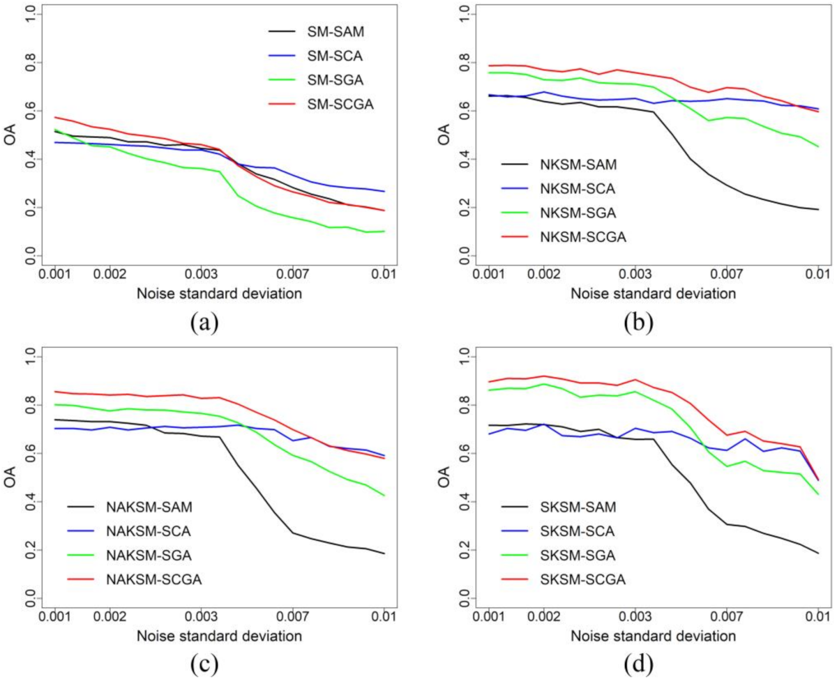
- In terms of the four matching methods, the proposed combined matching method can achieve promising mapping results at both high and low signal-to-noise ratios.
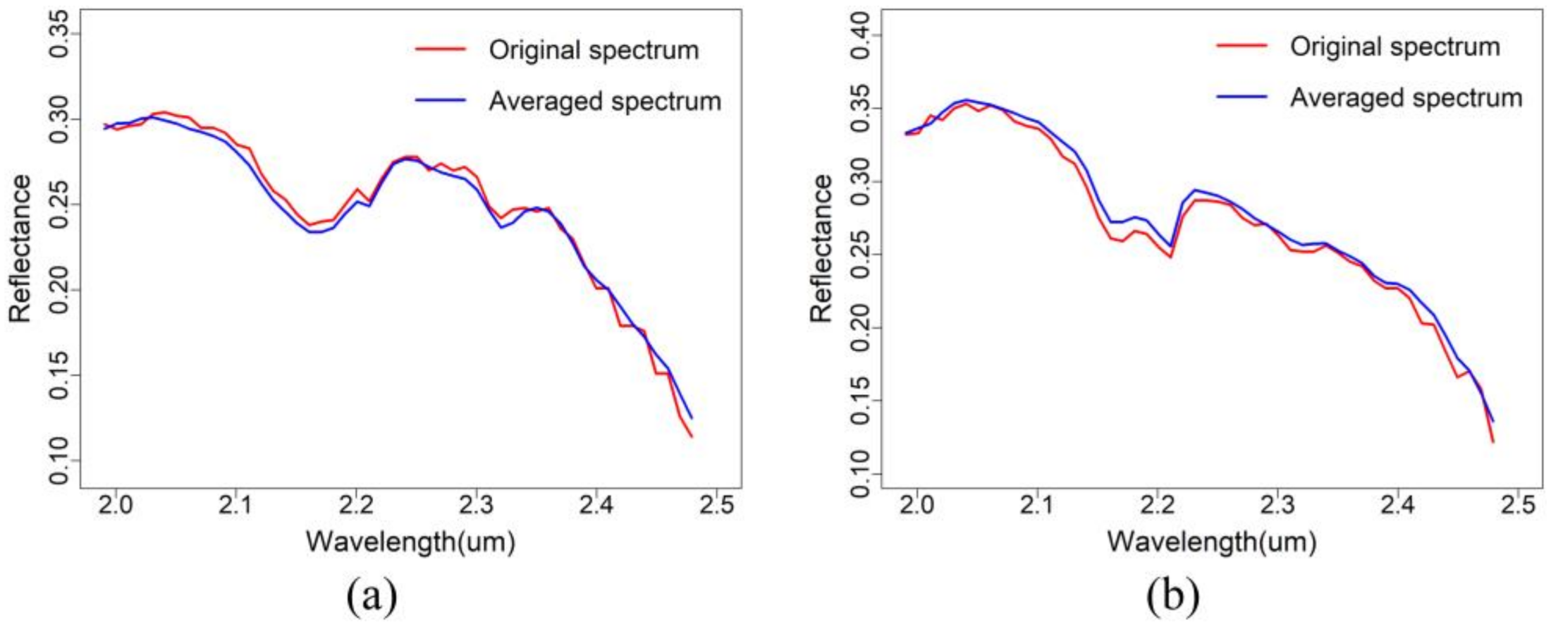
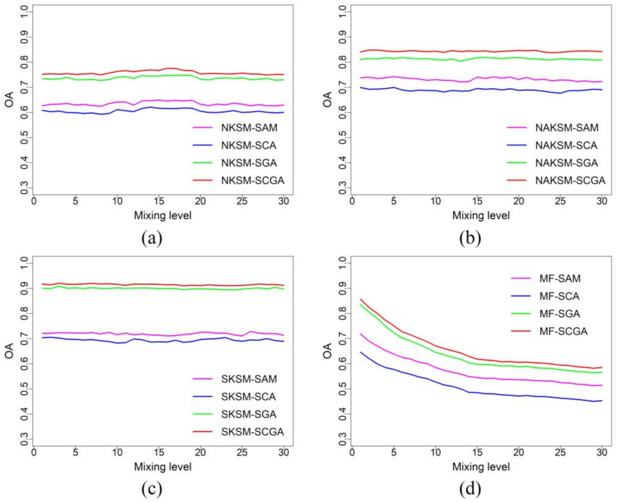
- In noise reduction, although both KSM and mean filtering remove noise by averaging, KSM does not blur out the details of the mineral mapping results and has a greater mapping efficiency. Most importantly of all, KSM is independent of the mixing of different mineral types.
Author Contributions
Funding
Institutional Review Board Statement
Informed Consent Statement
Data Availability Statement
Conflicts of Interest
Abbreviations
| The number of cluster centers | K |
| Spectral angle mapper | SAM |
| Spectral correlation angle | SCA |
| Spectral gradient angle | SGA |
| The matching method combing SCA and SGA | SCGA |
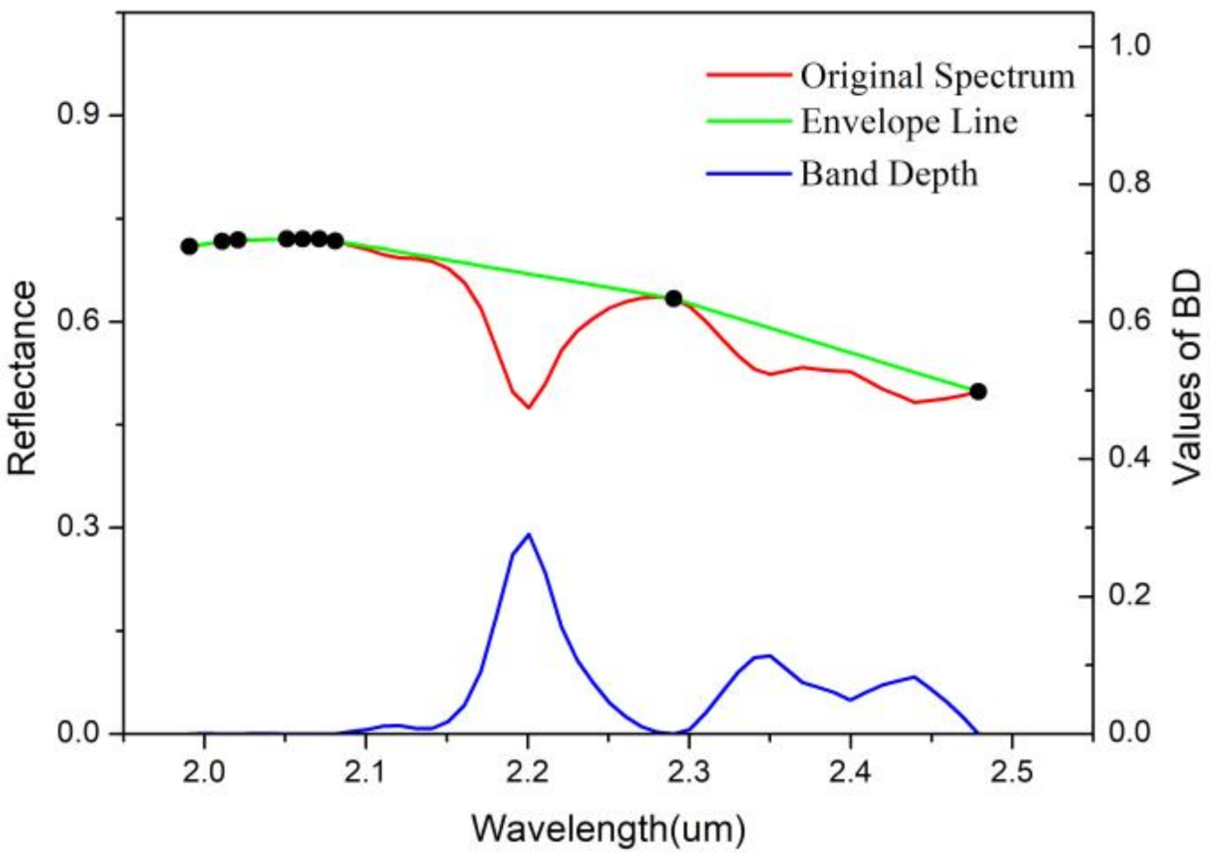
| Band depth | BD |
| Nonnegative matrix factorization | NMF |
| Singular value decomposition | SVD |
| Nonnegative Double Singular Value Decomposition | NNDSVD |
| The variant of NNDSVD | NNDSVDa |
| The NMF initialization method using spectral matching technology | SMNMF |
| Spectral matching | SM |
| The combination of k-means and SM | KSM |
| KSM mapping method based on NNDSVD | NKSM |
| KSM mapping method based on NNDSVDa | NAKSM |
| KSM mapping method based on SMNMF | SKSM |
References
- Ouahabi, M.E.; Daoudi, L.; Fagel, N. Mineralogical and geotechnical characterization of clays from northern Morocco for their potential use in the ceramic industry. Clay Miner. 2014, 49, 35–51. [Google Scholar] [CrossRef]
- Hojamberdiev, M.; Eminov, A.; Xu, Y. Utilization of muscovite granite waste in the manufacture of ceramic tiles. Ceram. Int. 2011, 37, 871–876. [Google Scholar] [CrossRef]
- Cordell, D.; Drangert, J.O.; White, S. The story of phosphorus: Global food security and food for thought. Glob. Environ. Change 2009, 19, 292–305. [Google Scholar] [CrossRef]
- Laakso, K.; Middleton, M.; Heinig, T.; Bärs, R.; Lintinen, P. Assessing the ability to combine hyperspectral imaging (HSI) data with Mineral Liberation Analyzer (MLA) data to characterize phosphate rocks. Int. J. Appl. Earth Obs. Geoinf. 2018, 69, 1–12. [Google Scholar] [CrossRef]
- Li, W.; Zhao, W.; Hu, Q. Effect of bifid triple viable tablets combined with montmorillonite powder on pediatric diarrhea and its influence on children’s immune function. Chin. Pediatr. Integr. Tradit. West. Med. 2018, 2, 150–152. [Google Scholar] [CrossRef]
- Ni, L.; Xu, H.; Zhou, X. Mineral Identification and Mapping by Synthesis of Hyperspectral VNIR/SWIR and Multispectral TIR Remotely Sensed Data with Different Classifiers. IEEE J. Sel. Top. Appl. Earth Observ. Remote Sens. 2020, 13, 3155–3163. [Google Scholar] [CrossRef]
- Vane, G.; Goetz, A.F.H. Terrestrial imaging spectrometry: Current status, future trends. Remote Sens. Environ. 1993, 44, 117–126. [Google Scholar] [CrossRef]
- Hubbard, B.E.; Crowley, J.K.; Zimbelman, D.R. Comparative alteration mineral mapping using visible to shortwave infrared (0.4-2.4 /spl mu/m) Hyperion, ALI, and ASTER imagery. IEEE Trans. Geosci. Remote Sens. 2003, 41, 1401–1410. [Google Scholar] [CrossRef]
- Meer, F.V.D.; Bakker, W. Cross correlation spectral matching: Application to surface mineralogical mapping using AVIRIS data from cuprite, Nevada. Remote Sens. Environ. 1997, 61, 371–382. [Google Scholar] [CrossRef]
- Yi, C.; Zhao, Y.Q.; Chan, J.C. Spectral Super-Resolution for Multispectral Image Based on Spectral Improvement Strategy and Spatial Preservation Strategy. IEEE Trans. Geosci. Remote Sens. 2019, 57, 9010–9024. [Google Scholar] [CrossRef]
- Acosta, I.C.C.; Khodadadzadeh, M.; Gloaguen, R. Resolution Enhancement for Drill-Core Hyperspectral Mineral Mapping. Remote Sens. 2021, 13, 2296. [Google Scholar] [CrossRef]
- Tompolidi, A.-M.; Sykioti, O.; Koutroumbas, K.; Parcharidis, I. Spectral Unmixing for Mapping a Hydrothermal Field in a Volcanic Environment Applied on ASTER, Landsat-8/OLI, and Sentinel-2 MSI Satellite Multispectral Data: The Nisyros (Greece) Case Study. Remote Sens. 2020, 12, 4180. [Google Scholar] [CrossRef]
- Jain, R.; Sharma, R.U. Airborne hyperspectral data for mineral mapping in Southeastern Rajasthan, India. Int. J. Appl. Earth Obs. Geoinf. 2019, 81, 137–145. [Google Scholar] [CrossRef]
- Cui, B.; Cui, J.; Hao, S.; Guo, N.; Lu, Y. Spectral-spatial Hyperspectral Image Classification Based on Superpixel and Multi-classifier Fusion. Int. J. Remote Sens. 2020, 41, 6157–6182. [Google Scholar] [CrossRef]
- Kang, X.; Duan, P.; Xiang, X.; Li, S.; Benediktsson, J.A. Detection and Correction of Mislabeled Training Samples for Hyperspectral Image Classification. IEEE Trans. Geosci. Remote Sens. 2018, 56, 5673–5686. [Google Scholar] [CrossRef]
- Hughes, G. On the mean accuracy of statistical pattern recognizers. IEEE Trans. Inf. Theory 1968, 14, 55–63. [Google Scholar] [CrossRef] [Green Version]
- Paoletti, M.E.; Haut, J.M.; Fernandez-Beltran, R.; Plaza, J.; Plaza, A.J.; Pla, F. Deep Pyramidal Residual Networks for Spectral-Spatial Hyperspectral Image Classification. IEEE Trans. Geosci. Remote Sens. 2019, 57, 740–754. [Google Scholar] [CrossRef]
- Iordache, M.; Bioucas-Dias, J.M.; Plaza, A. Collaborative Sparse Regression for Hyperspectral Unmixing. IEEE Trans. Geosci. Remote Sens. 2014, 52, 341–354. [Google Scholar] [CrossRef] [Green Version]
- Zhang, B.; Sun, X.; Gao, L.; Yang, L. Endmember Extraction of Hyperspectral Remote Sensing Images Based on the Ant Colony Optimization (ACO) Algorithm. IEEE Trans. Geosci. Remote Sens. 2011, 49, 2635–2646. [Google Scholar] [CrossRef]
- Chan, T.; Ma, W.; Ambikapathi, A.; Chi, C. A Simplex Volume Maximization Framework for Hyperspectral Endmember Extraction. IEEE Trans. Geosci. Remote Sens. 2011, 49, 4177–4193. [Google Scholar] [CrossRef]
- Dennison, P.E.; Halligan, K.Q.; Roberts, D.A. A comparison of error metrics and constraints for multiple endmember spectral mixture analysis and spectral angle mapper. Remote Sens. Environ. 2004, 93, 359–367. [Google Scholar] [CrossRef]
- Meer, F.V.D.; Bakker, W. CCSM: Cross Correlogram Spectral Matching. Int. J. Remote Sens. 1997, 18, 1197–1201. [Google Scholar] [CrossRef]
- Meer, F.V.D. The effectiveness of spectral similarity measures for the analysis of hyperspectral imagery. Int. J. Appl. Earth Obs. Geoinf. 2006, 8, 3–17. [Google Scholar] [CrossRef]
- Kumar, A.S.; Keerthi, V.; Manjunath, A.S.; Werff, H.V.D.; Meer, F.V.D. Hyperspectral image classification by a variable interval spectral average and spectral curve matching combined algorithm. Int. J. Appl. Earth Obs. Geoinf. 2010, 12, 261–269. [Google Scholar] [CrossRef]
- Tzortzis, G.; Likas, A. The minmax k-means clustering algorithm. Pattern Recognit. 2014, 47, 2505–2516. [Google Scholar] [CrossRef]
- Filippone, M.; Camastra, F.; Masulli, F.; Rovetta, S. A survey of kernel and spectral methods for clustering. Pattern Recognit. 2008, 41, 176–190. [Google Scholar] [CrossRef] [Green Version]
- Tompolidi, A.; Sykioti, O.; Koutroumbas, K.; Parcharidis, I. Detection of hydrothermal alteration on volcanic environments applying clustering on Landsat 8 OLI data. Case study: The Nisyros caldera (Greece). In Proceedings of the Conference HGS 2019: 12th International Conference of the Hellenic Geographical Society, Athens, Greece, 1–4 November 2019. [Google Scholar] [CrossRef]
- Klein, M.P.; Barton, G.W. Enhancement of signal-to-noise ratio by continuous averaging: Application to magnetic resonance. Rev. Sci. Instrum. 2004, 34, 754–759. [Google Scholar] [CrossRef]
- Micciancio, S. Noise reduction by averaging over the optical path in interferometry. Infrared Phys. Technol. 1977, 17, 67–70. [Google Scholar] [CrossRef]
- Manning, B.R.; Cochrane, C.J.; Lenahan, P.M. An improved adaptive signal averaging technique for noise reduction and tracking enhancements in continuous wave magnetic resonance. Rev. Sci. Instrum. 2020, 91, 033106. [Google Scholar] [CrossRef]
- Deledalle, C.A.; Denis, L.; Tupin, F. NL-InSAR: Nonlocal Interferogram Estimation. IEEE Trans. Geosci. Remote Sens. 2011, 49, 1441–1452. [Google Scholar] [CrossRef]
- Rodger, A.; Fabris, A.; Laukamp, C. Feature Extraction and Clustering of Hyperspectral Drill Core Measurements to Assess Potential Lithological and Alteration Boundaries. Minerals 2021, 11, 136. [Google Scholar] [CrossRef]
- Martel, E.; Lazcano, R.; López, J.; Madroñal, D.; Salvador, R.; López, S.; Juarez, E.; Guerra, R.; Sanz, C.; Sarmiento, R. Implementation of the Principal Component Analysis onto High-Performance Computer Facilities for Hyperspectral Dimensionality Reduction: Results and Comparisons. Remote Sens. 2018, 10, 864. [Google Scholar] [CrossRef] [Green Version]
- Nielsen, A.A. Kernel Maximum Autocorrelation Factor and Minimum Noise Fraction Transformations. IEEE Trans. Image Process. 2011, 20, 612–624. [Google Scholar] [CrossRef] [Green Version]
- Gao, L.; Zhao, B.; Jia, X.; Liao, W.; Zhang, B. Optimized Kernel Minimum Noise Fraction Transformation for Hyperspectral Image Classification. Remote Sens. 2017, 9, 548. [Google Scholar] [CrossRef] [Green Version]
- Lee, D.D.; Seung, H.S. Learning the parts of objects by nonnegative matrix factorization. Nature 1999, 401, 788–791. [Google Scholar] [CrossRef]
- Qiao, H. New SVD based initialization strategy for Nonnegative Matrix Factorization. Pattern Recognit. Lett. 2015, 63, 71–77. [Google Scholar] [CrossRef] [Green Version]
- Wild, S.; Curry, J.; Dougherty, A. Improving nonnegative matrix factorizations through structured initialization. Pattern Recognit. 2004, 37, 2217–2232. [Google Scholar] [CrossRef]
- Gong, L.; Nandi, A.K. An enhanced initialization method for non-negative matrix factorization. In Proceedings of the 2013 IEEE International Workshop on Machine Learning for Signal Processing (MLSP), Southampton, UK, 22–25 September 2013. [Google Scholar] [CrossRef] [Green Version]
- Li, T.; Ding, C. The Relationships Among Various Nonnegative Matrix Factorization Methods for Clustering. In Proceedings of the Sixth International Conference on Data Mining, Hong Kong, China, 18–22 December 2006; pp. 362–371. [Google Scholar] [CrossRef]
- Resmini, R.G.; Kappus, M.E.; Aldrich, W.S.; Harsanyi, J.C.; Anderson, M. Mineral mapping with Hyperspectral Digital Imagery Collection Experiment (HYDICE) sensor data at Cuprite, Nevada, U.S.A. Int. J. Remote Sens. 1997, 18, 1553–1570. [Google Scholar] [CrossRef]
- Siebels, K.; Gota, K.; Germain, M. Estimation of Mineral Abundance from Hyperspectral Data Using a New Supervised Neighbor-Band Ratio Unmixing Approach. IEEE Trans. Geosci. Remote Sens. 2020, 58, 6754–6766. [Google Scholar] [CrossRef]
- Clark, R.N.; Swayze, G.A.; Livo, K.E.; Kokaly, R.F.; Sutly, S.J.; Dalton, J.B.; McDougal, R.R.; Gent, C.A. Imaging spectroscopy: Earth and planetary remote sensing with the USGS Tetracorder and expert systems. J. Geophys. Res. Atmos. 2003, 108, 5131. [Google Scholar] [CrossRef]
- Chen, X.; Warner, T.A.; Campagna, D.J. Integrating visible, near-infrared and short-wave infrared hyperspectral and multispectral thermal imagery for geological mapping at cuprite, Nevada. Remote Sens. Environ. 2007, 110, 344–356. [Google Scholar] [CrossRef] [Green Version]
- Green, R.O.; Eastwood, M.L.; Sarture, C.M.; Chrien, T.G.; Aronsson, M.; Chippendale, B.J.; Faust, J.A.; Pavri, B.E.; Chovit, C.J.; Solis, M.; et al. Imaging Spectroscopy and the Airborne Visible/Infrared Imaging Spectrometer (AVIRIS). Remote Sens. Environ. 1998, 65, 227–248. [Google Scholar] [CrossRef]
- Kruse, F.A.; Boardman, J.W.; Huntington, J.F. Comparison of airborne hyperspectral data and EO-1 Hyperion for mineral mapping. IEEE Trans. Geosci. Remote Sens. 2003, 41, 1388–1400. [Google Scholar] [CrossRef] [Green Version]
- Carvalho, O.A.D.; Carvalho, A.P.F.; Guimaraes, R.F.; Lopes, R.A.S.; Guimaraes, P.A.; Martins, E.D.S.; Pedreno, J.N. Classification of hyperspectral image using SCM methods for geobotanical analysis in the Brazilian savanna region. In Proceedings of the IEEE International Symposium on Geoscience and Remote Sensing (IGARSS), Toulouse, France, 21–25 July 2003. [Google Scholar] [CrossRef]
- Ren, Z.; Sun, L.; Zhai, Q.; Liu, X. Mineral Mapping with Hyperspectral Image Based on an Improved K-Means Clustering Algorithm. In Proceedings of the IEEE International Symposium on Geoscience and Remote Sensing (IGARSS), Yokohama, Japan, 28 July–2 August 2019; pp. 2989–2992. [Google Scholar] [CrossRef]
- Noomen, M.F.; Skidmore, A.K.; Meer, F.V.D.; Prins, H.H.T. Continuum removed band depth analysis for detecting the effects of natural gas, methane and ethane on maize reflectance. Remote Sens. Environ. 2006, 105, 262–270. [Google Scholar] [CrossRef]
- Sykioti, O.; Paronis, D.; Stagakis, S.; Kyparissis, A. Band depth analysis of chris/proba data for the study of a mediterranean natural ecosystem correlations with leaf optical properties and ecophysiological parameters. Remote Sens. Environ. 2011, 115, 752–766. [Google Scholar] [CrossRef]
- Liu, X.; Xia, W.; Wang, B.; Zhang, L. An approach based on constrained nonnegative matrix factorization to unmix hyperspectral data. IEEE Trans. Geosci. Remote Sens. 2011, 49, 757–772. [Google Scholar] [CrossRef]
- Rezaei, M.; Boostani, R. An Efficient Initialization Method for Nonnegative Matrix Factorization. Appl. Sci. 2011, 11, 354–359. [Google Scholar] [CrossRef]
- Liu, H.W.; Li, X.L.; Zheng, X.Y. Solving nonnegative matrix factorization by alternating least squares with a modified strategy. Data Min. Knowl. Discov. 2013, 26, 435–451. [Google Scholar] [CrossRef]
- Xue, Y.; Tong, C.S.; Chen, Y.; Chen, W.S. Clustering-based initialization for nonnegative matrix factorization. Appl. Math. Comput. 2008, 205, 525–536. [Google Scholar] [CrossRef]
- Zhao, L.; Zhang, G.; Xu, X. Facial expression recognition based on PCA and NMF. In Intelligent Control and Automation; Scientific Research Publishing: Wuhan, China, 2008; pp. 6826–6829. [Google Scholar] [CrossRef]
- Atif, S.M.; Qazi, S.; Gillis, N. Improved SVD-based initialization for nonnegative matrix factorization using low-rank correction. Pattern Recognit. Lett. 2019, 122, 53–59. [Google Scholar] [CrossRef] [Green Version]
- Kitamura, D.; Ono, N. Efficient initialization for nonnegative matrix factorization based on nonnegative independent component analysis. In Proceedings of the 2016 IEEE International Workshop on Acoustic Signal Enhancement (IWAENC), Xi’an, China, 13–16 September 2016; pp. 1–5. [Google Scholar] [CrossRef]
- Pompili, F.; Gillis, N.; Absil, P.A.; Glineur, F. Two algorithms for orthogonal nonnegative matrix factorization with application to clustering. Neurocomputing 2014, 141, 15–25. [Google Scholar] [CrossRef] [Green Version]
- Li, X.; Cui, G.; Dong, Y. Graph Regularized Non-Negative Low-Rank Matrix Factorization for Image Clustering. IEEE Trans. Cybern. 2017, 47, 3840–3853. [Google Scholar] [CrossRef] [PubMed]
- Boutsidis, C.; Gallopoulos, E. SVD based initialization: A head start for nonnegative matrix factorization. Pattern Recognit. 2008, 41, 1350–1362. [Google Scholar] [CrossRef] [Green Version]
- Zhang, K.; Kwok, J.T. Clustered Nyström Method for Large Scale Manifold Learning and Dimension Reduction. IEEE Trans. Neural Netw. 2010, 21, 1576–1587. [Google Scholar] [CrossRef] [Green Version]
- Du, H.; Wang, Y.; Duan, L. A New Method for Grayscale Image Segmentation Based on Affinity Propagation Clustering Algorithm. In Proceedings of the 2013 Ninth International Conference on Computational Intelligence and Security, Emeishan, China, 14–15 December 2013; pp. 170–173. [Google Scholar] [CrossRef]
- Likas, A.; Vlassis, N.; Verbeek, J.J. The global k-means clustering algorithm. Pattern Recognit. 2003, 36, 451–461. [Google Scholar] [CrossRef] [Green Version]
- Pena, J.M.; Lozano, J.A.; Larranaga, P. An empirical comparison of four initialization methods for the k-means algorithm. Pattern Recognit. Lett. 1999, 20, 1027–1040. [Google Scholar] [CrossRef]
- Kumar, P.; Gupta, D.K.; Mishra, V.N.; Prasad, R. Comparison of Support Vector Machine, Artificial Neural Network, and Spectral Angle Mapper Algorithms for Crop Classification Using LISS IV Data. Int. J. Remote Sens. 2015, 36, 1604–1617. [Google Scholar] [CrossRef]
- Angelopoulou, E.; Lee, S.W.; Bajcsy, R. Spectral gradient: A material descriptor invariant to geometry and incident illumination. In Proceedings of the Seventh IEEE International Conference on Computer Vision, Kerkyra, Greece, 20–27 September 1999. [Google Scholar] [CrossRef]
- Carvalho, O.A.; Meneses, P.R. Spectral Correlation Mapper (SCM): An Improvement on the Spectral Angle Mapper (SAM). In Summaries of the Ninth Annual JPL Airborne Earth Science Workshop, February 23–25, 2000; JPL: Pasadena, CA, USA, 2000. [Google Scholar]
- Congalton, R.G. A review of assessing the accuracy of classifications of remotely sensed data. Remote Sens. Environ. 1991, 37, 35–46. [Google Scholar] [CrossRef]


| Matching Method | SM | NKSM | NAKSM | SKSM |
|---|---|---|---|---|
| SAM | 0.5167 | 0.6441 | 0.7375 | 0.7329 |
| SCA | 0.4955 | 0.6296 | 0.6954 | 0.7102 |
| SGA | 0.5431 | 0.7517 | 0.8120 | 0.8966 |
| SCGA | 0.6005 | 0.7772 | 0.8580 | 0.9282 |
| Time (sec) | SM | NKSM | NAKSM | SKSM |
|---|---|---|---|---|
| SAM | 201.8196 | 99.5971 | 136.1710 | 86.7398 |
| SCA | 1812.1085 | 102.4428 | 142.2040 | 90.5664 |
| SGA | 187.2481 | 97.6556 | 134.8296 | 85.6867 |
| SCGA | 2079.9541 | 104.1109 | 155.0557 | 92.2011 |
| Total | 4281.1302 | 403.8064 | 568.2603 | 355.1941 |
Publisher’s Note: MDPI stays neutral with regard to jurisdictional claims in published maps and institutional affiliations. |
© 2022 by the authors. Licensee MDPI, Basel, Switzerland. This article is an open access article distributed under the terms and conditions of the Creative Commons Attribution (CC BY) license (https://creativecommons.org/licenses/by/4.0/).
Share and Cite
Ren, Z.; Zhai, Q.; Sun, L. A Novel Method for Hyperspectral Mineral Mapping Based on Clustering-Matching and Nonnegative Matrix Factorization. Remote Sens. 2022, 14, 1042. https://doi.org/10.3390/rs14041042
Ren Z, Zhai Q, Sun L. A Novel Method for Hyperspectral Mineral Mapping Based on Clustering-Matching and Nonnegative Matrix Factorization. Remote Sensing. 2022; 14(4):1042. https://doi.org/10.3390/rs14041042
Chicago/Turabian StyleRen, Zhongliang, Qiuping Zhai, and Lin Sun. 2022. "A Novel Method for Hyperspectral Mineral Mapping Based on Clustering-Matching and Nonnegative Matrix Factorization" Remote Sensing 14, no. 4: 1042. https://doi.org/10.3390/rs14041042
APA StyleRen, Z., Zhai, Q., & Sun, L. (2022). A Novel Method for Hyperspectral Mineral Mapping Based on Clustering-Matching and Nonnegative Matrix Factorization. Remote Sensing, 14(4), 1042. https://doi.org/10.3390/rs14041042