Global Mangrove Watch: Updated 2010 Mangrove Forest Extent (v2.5)

Abstract

This study presents an updated global mangrove forest baseline for 2010: Global Mangrove Watch (GMW) v2.5. The previous GMW maps (v2.0) of the mangrove extent are currently considered the most comprehensive available global products, however areas were identified as missing or poorly mapped. Therefore, this study has updated the 2010 baseline map to increase the mapping quality and completeness of the mangrove extent. This revision resulted in an additional 2660 km² of mangroves being mapped yielding a revised global mangrove extent for 2010 of some 140,260 km². The overall map accuracy was estimated to be 95.1% with a 95th confidence interval of 93.8–96.5%, as assessed using 50,750 reference points located across 60 globally distributed sites. Of these 60 validation sites, 26 were located in areas that were remapped to produce the v2.5 map and the overall accuracy for these was found to have increased from 82.6% (95th confidence interval: 80.1–84.9) for the v2.0 map to 95.0% (95th confidence interval: 93.7–96.4) for the v2.5 map. Overall, the improved GMW v2.5 map provides a more robust product to support the conservation and sustainable use of mangroves globally.

1. Introduction

At the United Nations Framework Convention on Climate Change (UNFCCC) Conference of the Parties 26 (COP26) in 2021, an international agreement was made to end deforestation by 2030. To ensure adherence to this, accurate global scale maps of forested ecosystems will be critical. One such ecosystem is mangrove forests, which have witnessed an elevated rate of loss compared to terrestrial forests over the past decades [1] with regional losses exceeding 3%, driven by anthropogenic disturbances [1,2,3] such as conversion to aquaculture [4] or agriculture [5], urban expansion [6], oil palm plantations [7], and climate change [8]. Mangrove forests support a large number of ecosystem services [9], such as carbon storage and sequestration [10], coastal protection [11], food production [9], and tourism [12]. The ecosystem services of tidal mangroves and marshes were estimated to be worth 193,843 USD per hectare per year for 2007, equating to 25 trillion USD annually [13]. Accurate baseline maps of extent are therefore essential for a local and global ecosystem service accounting as well as verifying COP26 goals. Indeed, the ambitious goals set by the Global Mangrove Alliance (GMA), to restore 20% of mangrove forests by 2030, require accurate baselines upon which their efforts can be built. Furthermore, baseline maps are the keystone for mapping environmental descriptors that characterise this ecosystem, such as biomass [14], understanding the drivers of land cover change [2], and locating primary regions for potential restoration.

The Bunting et al. [15] Global Mangrove Watch (GMW) version 2.0 extent maps have emerged as the primary global dataset for characterising mangrove extent. There are a number of initiatives (e.g., GMA, GMW Portal; https://globalmangrovewatch.org; accessed 8 January 2022) that are aiming to preserve and restore mangroves and wider international objectives such as the UN Sustainable Development Goals (SDGs), for which the existing Global Mangrove Watch (GMW) version 2.0 layers [15,16] are a key dataset and are already used for reporting against. Currently, the GMW v2.0 [16] is the most up-to-date mangrove extent at the highest spatial resolution available. However, all mangrove datasets (i.e., [15,16,17,18]) published to date have areas that are missing (i.e., not mapped) or where mapping quality is poor. These limitations are evident globally and are caused by, for example, sensor specific characteristics (e.g., Landsat 7 Enhanced Thematic Mapper (ETM+) scan-line error), limited data availability, excessive cloud cover, or a combination of the above. These limitations degrade the performance of the map to meet the needs of the COP26 and GMA global initiatives by the year 2030.

For the GMW version 2.0, Bunting et al. [15] used two random forest classifiers to classify mangrove extent for the year 2010 from a combination of ALOS PALSAR and Landsat sensor data. As demonstrated by [15,19,20], the L-band radar data used in GMW v2.0 are sensitive to mapping mangrove change, while providing limited capability to classify the mangrove extent. However, optical remotely sensed data, particularly those with a Shortwave Infrared (SWIR) waveband, are well suited to the mapping of mangrove forest extent [21]. More recently, a number of studies (e.g., [21,22,23,24,25]) have made use of Sentinel-2 imagery and have demonstrated typical classification accuracies >90% for mangrove extent using ensemble machine learning classification approaches (e.g., random forests) through the Google Earth Engine platform. However, these studies have typically been undertaken over small spatial extents or for a few countries (e.g., [25]), single countries (e.g., [24]), or particular areas of interest at sub-national scales (e.g., [23]). Alternative approaches to mangrove mapping that have focused on mapping through time have also been proposed, such as [26,27], which have used the COntinuous monitoring of Land Disturbance (COLD) [28] method to provide individual site level time-series maps of mangrove extent. However, these time-series approaches are computationally intensive and therefore difficult to apply at a global scale. Nevertheless, they have demonstrated the ability of advanced machine learning and intensive computational processing for delivering maps at the quality required for international reporting.

The aim of this work was to produce an update to the 2010 Global Mangrove Watch version 2.0 [15] suitable for fully supporting the needs of ambitious global level targets relating to mangrove forest preservation and restoration. Specific regions were identified as missing or of poor quality within the GMW v2.0 product and a new method was, therefore, proposed for achieving vastly improved mapping, combining higher-resolution data at higher imaging cadence with advanced machine learning models. These results were combined with the GMW v2.0 map to create the most complete map of mangrove extent currently available and will form the basis of a subsequent study, updating the estimates of mangrove change.

2. Materials and Methods

The analysis was undertaken on the SuperComputing Wales (SCW) High Performance Computing (HPC) infrastructure using the Remote Sensing and GIS Library (RSGISLib) of tools [29], the KEA image format [30] and the pbprocesstools [31] workload management library to manage the workflow of tasks on the HPC.

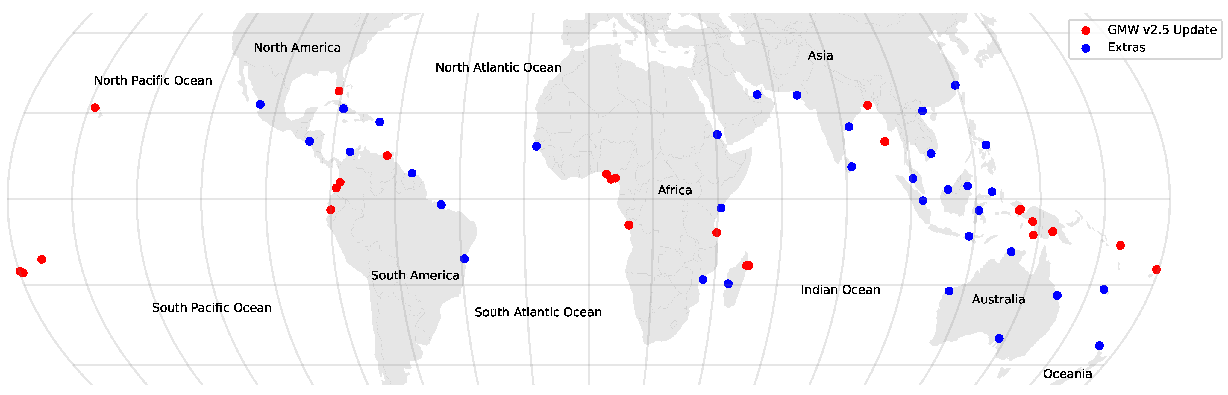
2.1. Areas to Be Mapped

Through user feedback on the GMW v2.0 maps, 204 regions were identified to be either missing or poorly mapped. As detailed by Bunting et al. [15], the choice of 2010 for the baseline map was driven by the use of ALOS PALSAR data, coverage of which was most complete for the year 2010 [15]. However, this resulted in Landsat-5 TM and Landsat-7 ETM+ temporal composites affected by ETM+ scan-line error artefacts, particularly in areas of high cloud cover (e.g., Niger Delta). These artefacts were, in some cases, present with the GMW v2.0 maps. Areas identified that required (re-)mapping as part of this study are shown in Figure 1.

2.2. Mangrove Habitat Mask

Bunting et al. [15] developed a mangrove habitat mask which was used to limit the classification of mangroves to those where mangroves can be expected to be present. For example, mangroves must generally be close to water and at or close to mean sea level. However, this mask was found to have been too tight in a number of regions (e.g., Florida, USA) and therefore caused under-classification of mangroves. Ahead of the mapping, the habitat mask was therefore revised, primarily through manually digitising regions to be added, but also intersecting the maps of [17,18] to ensure that all regions mapped in those products were fully located within the GMW habitat mask.

2.3. Mangrove Mapping

Bunting et al. [15] used the most appropriate and available data (i.e., Landsat TM and ETM+ and ALOS PALSAR) for 2010 in the original mapping (v2.0). Therefore, to improve the mapping, an approach that used alternative datasets was required. In this case, Sentinel-2 imagery was used to map the areas outlined in Figure 1. For the analysis, 100 global mangrove/non-mangrove XGBoost classifiers [32] were trained and applied to each Sentinel-2 acquisition. To produce a single unified classification, results from all acquisitions and classifiers were merged to create a probability for each pixel to be mangroves. This probability surface was then thresholded to produce the binary map, which was subject to a manual Quality Assurance (QA) process to produce the Sentinel-2-derived maps. These were then combined with the v2.0 2010 baseline and a change detection using the 2010 ALOS PALSAR data was applied to create a revised GMW v2.5 2010 baseline. The processing stages are outlined in Figure 2.

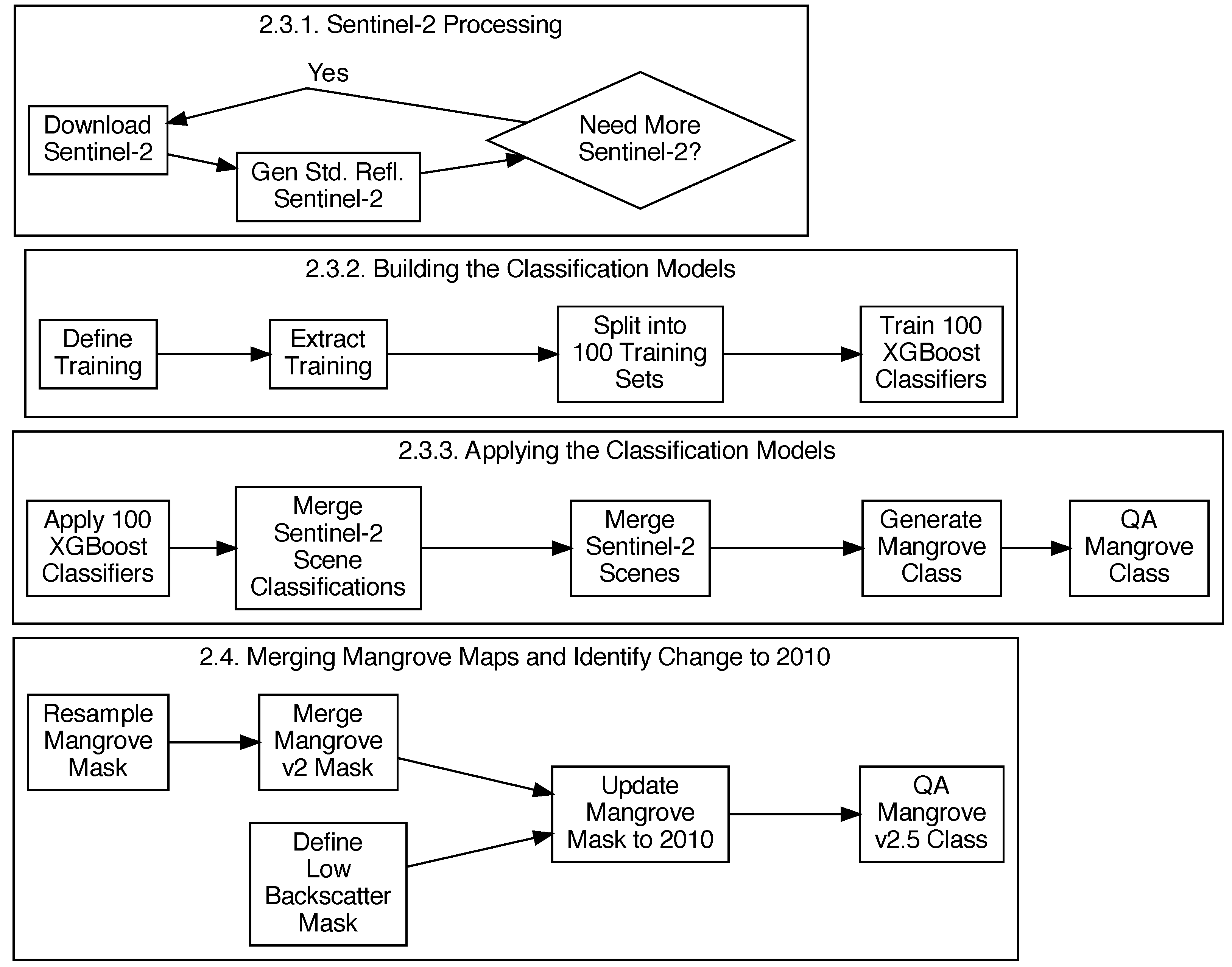
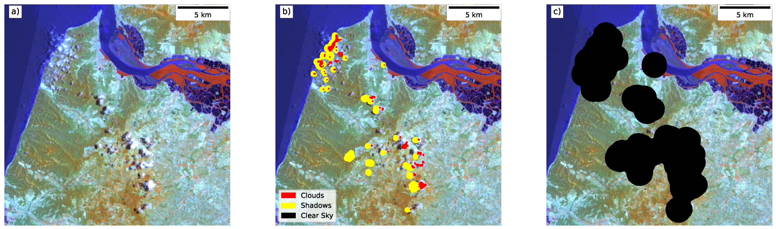
2.3.1. Sentinel-2 Processing

The Sentinel-2 imagery was downloaded from the Google Cloud public dataset [33] and, for the purpose of this work, processed to a 20-m pixel resolution (i.e., the 10-m resolution Sentinel-2 image bands were resampled to 20 m using averaging) orthorectified standardised surface reflectance product. For the 383 Sentinel-2 granules identified as intersecting with the regions of interest (Figure 1), individual acquisitions were selected for download based on cloud cover. Initially, the 10 acquisitions with the lowest cloud cover (maximum cloud cover of 20%) were identified from the entire Sentinel-2 archive (2015–2020). An iterative process was then followed where, for each granule, the scenes were downloaded and processed to produce a cloud mask. The combined cloud masks were checked to estimate whether data were available for all mangrove regions within the scene, as defined by the mangrove habitat mask. If more acquisitions were required, the thresholds for the number of acquisitions and maximum cloud cover were increased. These were increased to a maximum of 100 scenes and a maximum cloud threshold of 75%. In total, 11,262 Sentinel-2 acquisitions were downloaded and used for this analysis.

To generate a standardised reflectance product for the classifications, the ARCSI software [34] was employed, as successfully demonstrated in past studies [15,26,27,35]. The ARCSI software uses the 6S model [36] through the Py6S module [37] parameterised using the image header information and an aerosol optical depth estimated from a dark object subtraction [15]. Using the method of Shepherd and Dymond [38], the resulting images were normalised for a sensor view angle and local topography producing a standardised reflectance product. A tropical atmosphere and maritime aerosol profile was used for all scenes.

Cloud masking was undertaken using the product of two approaches. The FMask [39,40] algorithm was applied using the Python-FMask implementation [41]. The s2cloudless [42] LightGBM classifier [43] was also applied to each scene. The resulting s2cloudless classification was further refined using a morphological closing (with a $5\times 5$ circular operator) followed by a morphological dilation (with a $7\times 7$ circular operator). Finally, any cloud objects were removed if they were less than 10 pixels in size. The final cloud mask was defined as the intersection of the two masks. The cloud shadow mask was derived using the approach implemented within FMask, as described in Zhu et al. [39].

Finally, a ‘clear sky’ mask was derived for each acquisition, defining the areas of the scene to be used for further analysis. The ‘clear-sky’ mask aims to identify the larger continuous parts of the image, removing small areas between clouds. The first step buffered the cloud and cloud shadows by 30 km, clumping the remaining non-cloud regions. The non-cloud clumps with an area greater than 3000 pixels were then selected and grown to the 10-km contour of the cloud and cloud shadow pixels. An example of the ‘clear sky’ mask is shown in Figure 3c.

2.3.2. Building the Classification Models

Classification of mangrove extent was undertaken on a scene-by-scene basis rather than through the creation of image composites (i.e., merging multiple scenes using a metric such as the greenest pixel). Image composites, whilst relevant for visualisation, often have artefacts due to prevailing environmental conditions (e.g., wet or dry season or, in the case of mangroves, tidal regimes) at the time of the acquisitions or processing errors (e.g., missed cloud or cloud shadows). These artefacts can then impact the classification result. An alternative is to classify each of the scenes independently and then merge those results to create a single map.

To derive training data for the classification, 10,284 samples were created from the existing GMW v2.0 map. These were manually checked against the Sentinel-2 imagery. For regions not already within the GMW v2.0 product training regions, these were manually defined. Non-mangrove regions were defined as regions outside of the GMW habitat product, with points sampled randomly within this region and through manual selection of regions giving a total of 52,555 sample points for training.

The resulting samples were then intersected with all 11,262 Sentinel-2 acquisitions, with each scene masked to the relevant valid clear sky area. This resulted in 4,421,644 mangrove and 9,830,388 non-mangrove pixel values to train the classifier. Given the volume of sample data available, it was decided to split the training data into 100 sets, each with 400,000 samples (200,000 for mangroves and 200,000 for non-mangroves). Those samples were then split into 3 sets for training (100,000 for each class), testing (50,000 for each class), and validating (50,000 for each class) the model.

The XGBoost [32] binary classification algorithm was used for the analysis given its ability to use large training datasets and allow transfer learning (i.e., further training of an existing model). This method has been shown by John et al. [35] to provide good results for the classification of land cover from Earth observation data. To optimise the hyper-parameters of the XGBoost model, a subset of 20% was selected from the training (20,000 per class) and validation (10,000 per class) samples. Bayesian optimisation was used to identify the optimal hyper-parameters for each of the 100 classifiers. The range of values for the parameters optimised is given in

Table 1. The range of hyper-parameter values from the 100 models.

Parameter	Min.	Low. Quartile	Median	Up. Quartile	Max.	Mode
eta	0.0835	0.236	0.299	0.299	0.489	0.299
gamma	0	0	0	4	4	0
max_delta_step	0	6	7	7	10	7
max_depth	8	13	13	16	20	13
min_child_weight	1	10	10	10	10	10
num_boost_round	68	100	100	100	100	100
subsample	0.752	0.818	0.839	1.0	1.0	0.818

. Following identification of the hyper-parameters, each of the 100 models was trained using the full dataset (i.e., 400,000 samples). The testing accuracies of the models (using the 50,000 samples per class) were between 97–99%.

2.3.3. Applying the Classification Models

To apply the 100 global XGBoost classifiers to the individual Sentinel-2 acquisitions, the models were first further trained using the local training data from the Sentinel-2 acquisition, which was limited to 25,000 samples. This allowed the global classifier to be locally optimised for the individual acquisitions. The classifiers were then applied to all the acquisitions, with this creating 112,620 classifications. To avoid incorrect classification of mangroves in areas where they would not be located (e.g., in mountainous areas), the classification was only applied within an updated version of the mangrove habitat layer of Bunting et al. [15].

The individual classifications were then merged in two steps to create a mangrove probability for each pixel. The first step merged the 100 classifications applied to a scene to create a single probability output image for the scene. The probability was calculated as the number of times each pixel had been classified as mangroves (i.e., a value of 1 meant that all 100 classifiers classified the pixel as mangroves, while a value of 0.1 meant that only 10 classifiers classified the pixel as mangroves). The second step calculated the mean probability from all the acquisitions for each pixel, providing a single probability surface for all the areas mapped.

To derive the final binary mask of mangrove extent, a global threshold was applied to the probability surface. The threshold was identified through a sensitivity analysis using the mangrove samples based on the 0.1 increments (from 0.2 to 0.8). A mangrove mask was generated for each threshold where the mask with the best agreement with the mangrove samples used to train and test the XGBoost classifiers selected. A threshold of 0.5 provided the greatest correspondence and was therefore applied to all the regions updated using the Sentinel-2 imagery. For studies focused on specific regions, a further local optimisation could be undertaken by selecting a local threshold. However, for this study, a global threshold was applied as defining local regions would be difficult and could result in boundary artefacts within the resulting maps.

Finally, a visual assessment of the mangrove extent was undertaken where polygons identifying regions as incorrectly classified as mangroves were digitised with reference to the Sentinel-2 imagery and high-resolution Google Earth, Mapbox Satellite, and Bing maps imagery. The areas were then removed from the mangrove extent mask.

2.4. Merging Mangrove Maps and Identify Change to 2010

In addition to the new map produced from the Sentinel-2 analysis, two other mangrove maps were used to resolve issues for particular areas. For the Sundarbans, in India and Bangladesh, the mapping of Awty-Carroll et al. [26] for the year 2010 was added to the Sentinel-2 maps to be merged with the GMW v2.0 products. The Sundarbans were significantly affected by stripping from the Landsat ETM+ data within GMW v2.0. Additionally, mangrove maps for the French overseas territories, where there was found to be a high prevalence of cloud cover that reduces the availability of useable Sentinel-2 data, generated by the French National Mangrove Observation Network [44], were used to improve the new maps.

Following generation of the revised maps, these were merged with the existing GMW v2.0 baseline for 2010 to create the updated 2010 GMW v2.5 baseline. However, the updated areas had been mapped with data acquired over the period from 2015 to 2020 and a change detection was therefore required to backcast the map for 2010. 2010 ALOS PALSAR data were used for this and therefore the new mapping was resampled (nearest neighbour) onto the same 0.000222 degrees (∼25 m) pixel grid of the GMW v2.0 and ALOS PALSAR data layers.

As demonstrated by Thomas et al. [3,19,20], mangroves produce a high backscatter response in the L-band SAR data while the majority of non-mangrove surfaces (e.g., water bodies and mudflats) have a low L-band backscatter. As a result, there is a change trajectory between mangroves and non-mangroves, which was used by Thomas et al. [20] as the basis for a methodology for mapping mangrove change. This was applied globally to produce the GMW v2.0 change layers [16].

For implementation, a low backscatter mask was created for 2010 and used to remove mangroves that were within the new map but not present in 2010. The mask was defined using a combination of the ALOS PALSAR 2010 layer and the Landsat-based Pekel et al. [45] water occurrence layer generated for the period 1984–2020. The analysis was undertaken on a $1\times 1$ degree grid, where the water occurrence layer was used to define areas that could be considered as ‘permanent’ waterbodies, defined as a water occurrence between >90 and <100. However, if no pixels were identified, then the threshold was lowered to >70. For the pixels associated with ‘permanent’ waterbodies, the 99th percentile of the SAR backscatter was calculated for both the Horizontal-Horizontal (HH) and Horizontal-Vertical (HV) polarisations. The thresholds for classifying the water extent were then calculated for both polarisations as:

$$\mathrm{SAR}\mathrm{threshold}=99\mathrm{th}\mathrm{percentile}-(0.15\times 99\mathrm{th}\mathrm{percentile}).$$

(1)

If no ‘permanent’ waterbody pixels were identified, then the SAR thresholds where defined as $-14$ dB in the HH and $-17$ dB in the HV polarisations. To produce the low backscatter mask, the SAR backscatter was thresholded with values below those calculated above were used and the water occurrence layer had a value $>5$.

The low backscatter mask was then used to mask all the tiles, including areas which have not been remapped, updating the mangrove mask and aligning it with the ALOS PALSAR data for 2010. Finally, a Quality Assurance (QA) process was undertaken where the product was visually assessed against a variety of image sources, including high-resolution Google Earth, Mapbox Satellite and Bing Maps imagery, the Sentinel-2 data, 2010 ALOS PALSAR, and 2010 Landsat imagery data. Polygons were manually drawn for regions which should be removed from the map (i.e., not mangroves but areas that had been mapped as mangroves) or added to the map (i.e., mangroves but areas that had not been mapped as such). These QA edits were then rasterised and applied to the map producing the final GMW v2.5 layer.

2.5. Accuracy Assessment

To assess the accuracy of the new v2.5 layer, 26 sites (Figure 4) where new mapping had occurred were selected, representing a range of different mangrove settings, types, and extents. Additionally, a further 34 sites (Figure 4) were distributed globally for assessing the overall product accuracy. For each site, an area of $0.2\times 0.2$ degrees was defined and 1000 random stratified points were defined for each class (mangroves and non-mangroves). If there were less than 1000 mangrove pixels within the $0.2\times 0.2$ degree area then all mangrove pixels were defined as points and the number of mangrove reference points was reduced. The 2000 points were then split into 200 point sets (i.e., 100 mangrove and 100 non-mangrove) where the sets were assessed in turn until the 95% confidence interval for the macro F1-score was <5%. A minimum of 3 sets (i.e., 600 points) were assessed for each site, where typically 5 sets were required (1000 points) although 10 sets were used for one site. Points were manually annotated with a reference class through a combination of high-resolution Google Earth, Mapbox Satellite and Bing Maps imagery, the Sentinel-2 and 2010 ALOS PALSAR, and Landsat imagery data. In total, 50,750 points were assessed and used for the accuracy assessment. For sites where the mapping was updated, the points were also used to assess the improvement in map accuracy achieved through this study.

3. Results

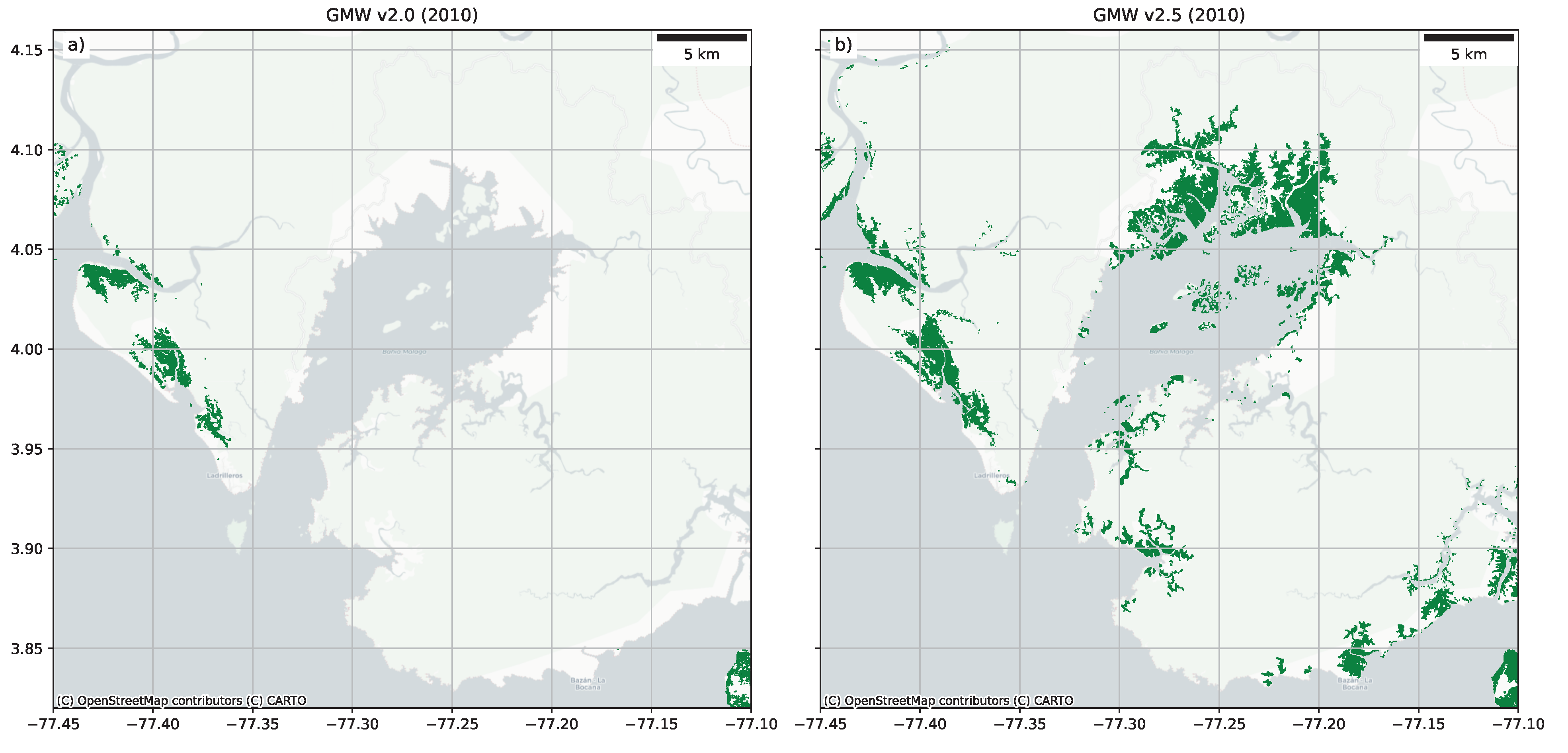
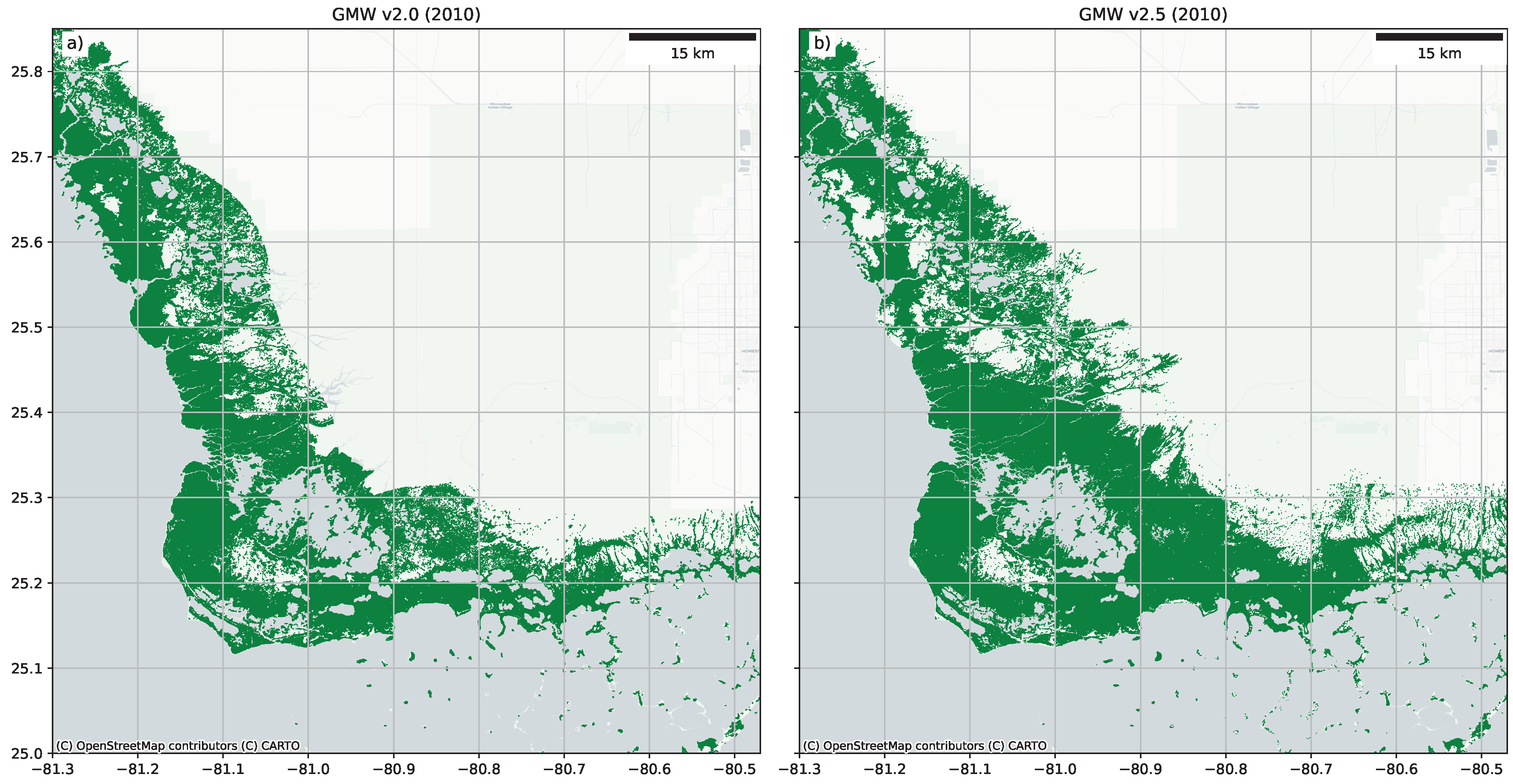
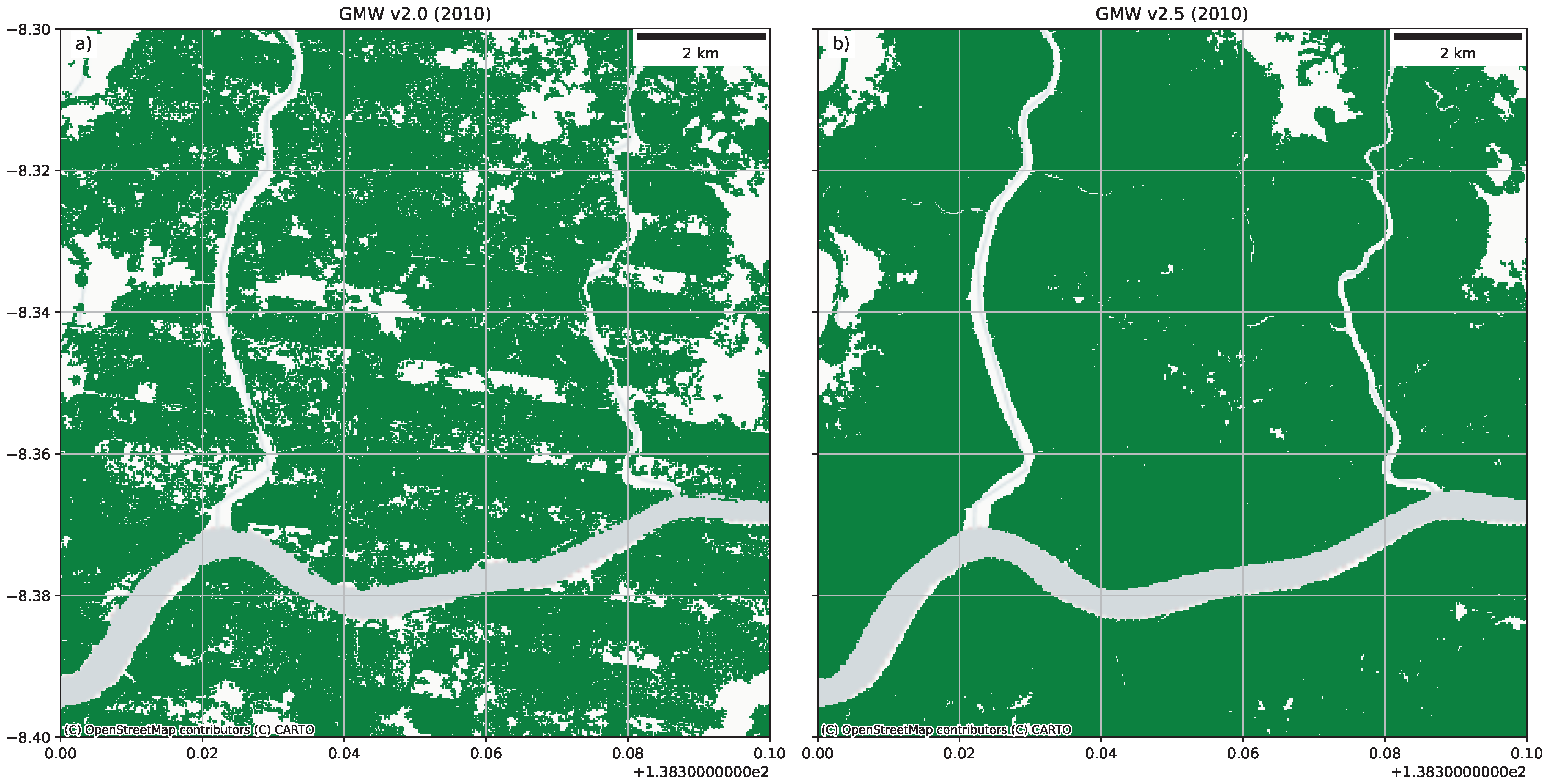
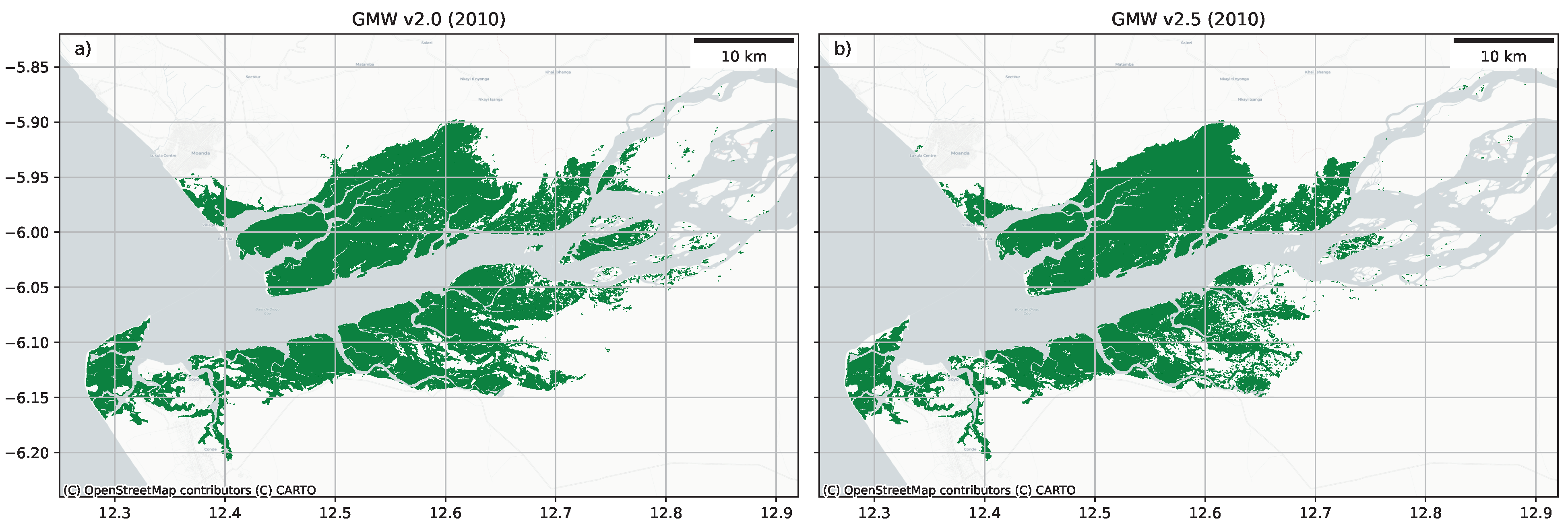
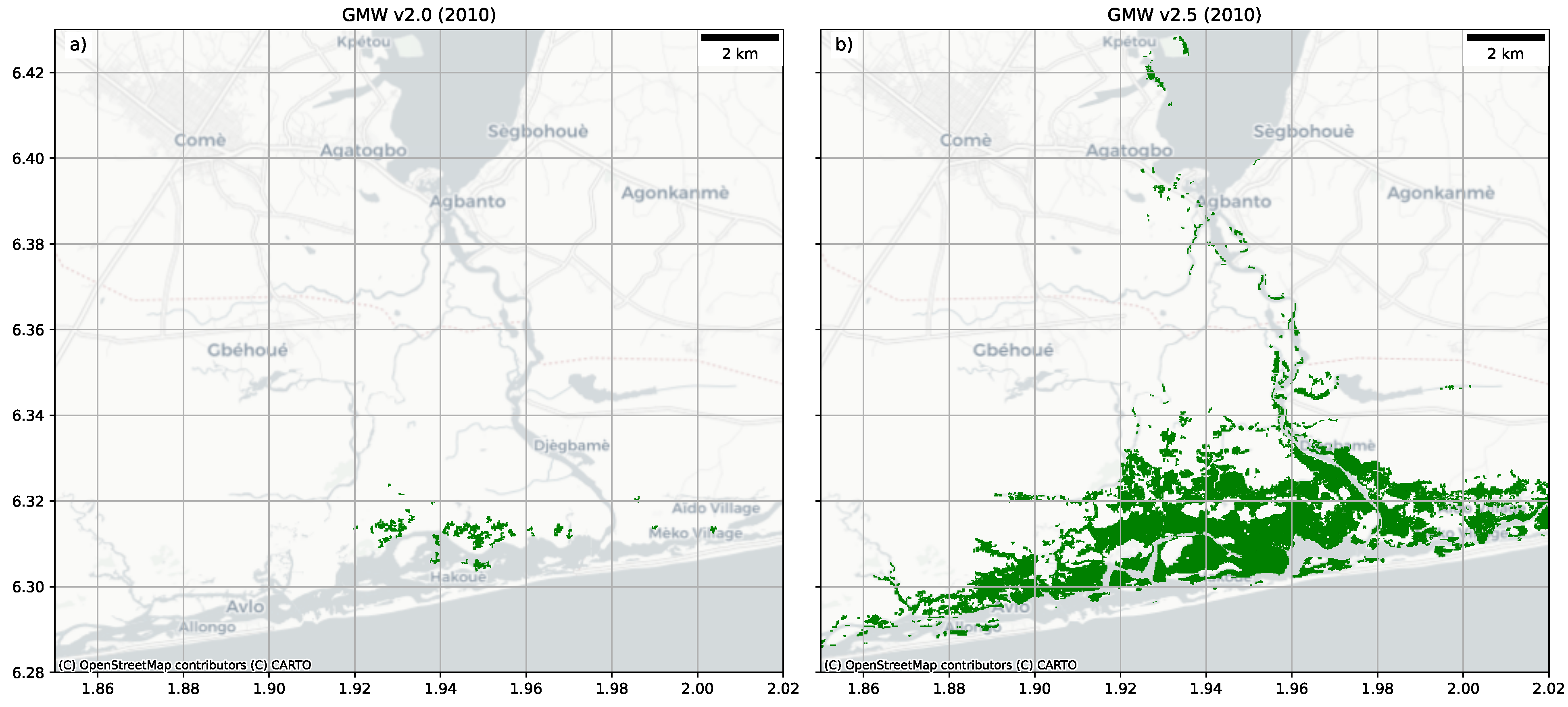
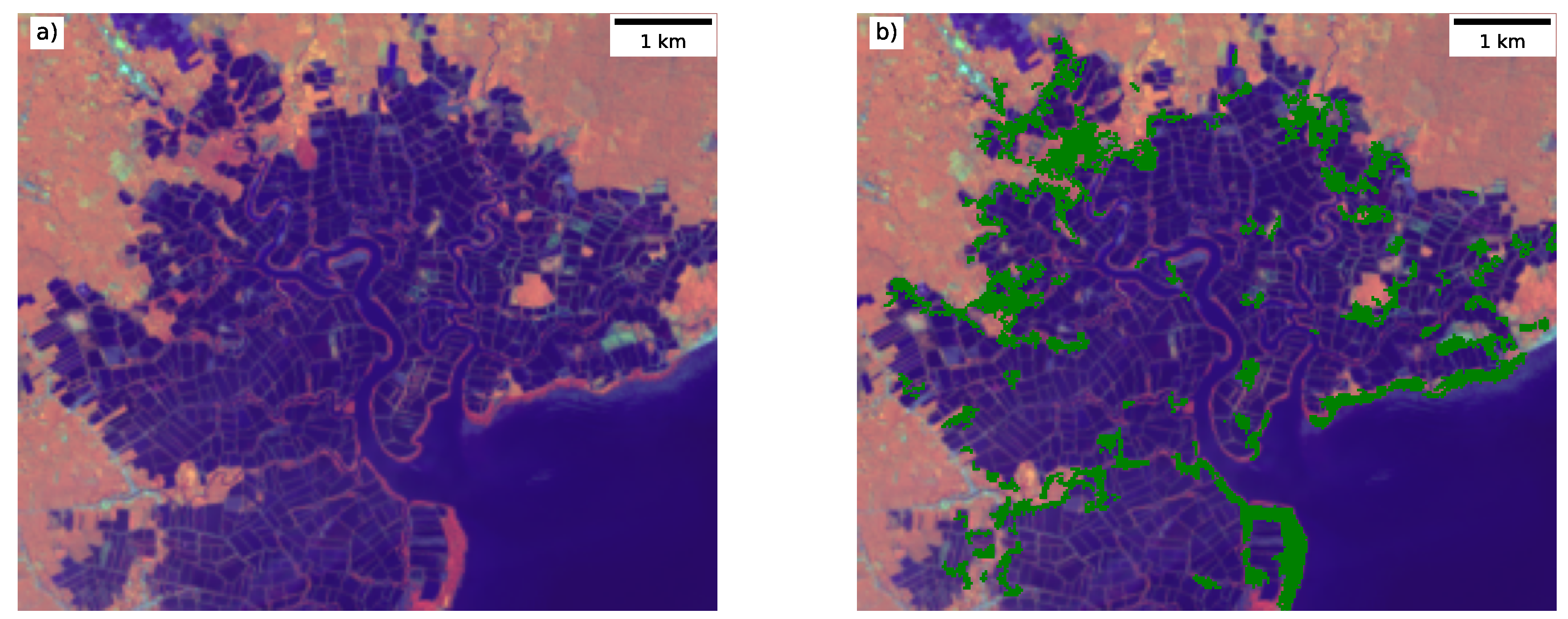
3.1. Remapped Regions Comparison

To compare the accuracy of the updated v2.5 and v2.0 GMW 2010 baselines, the reference points for the 26 sites where the baseline has been updated were intersected with both layers. Summary statistics calculated were an overall accuracy, cohen kappa, and F1 score (per-class and overall), with summaries are provided in

Table 2. For the region mapped to create v2.5, this table contains an overview of the accuracy statistics from the GMW v2.0 baseline, which can be compared to the statistics in Table 3.

Stats (GMW V2.0)	Overall	95th Confidence	Site Median	Site Min	Site Max
Overall (%)	82.6	80.1–84.9	84.8	51.6	96.3
Kappa	0.655	0.607–0.698	0.734	0.393	0.927
Macro F1-Score	0.824	0.799–0.847	0.866	0.334	0.963
Mangrove F1-Score	0.807	0.777–0.834	0.848	0.603	0.964
Mangrove Recall	0.706	0.665–0.746	0.774	0.437	0.976
Mangrove Precision	0.942	0.916–0.964	0.952	0.747	0.994
Other F1-Score	0.841	0.817–0.860	0.885	0.668	0.964
Other Recall	0.953	0.934–0.971	0.976	0.628	1.0
Other Precision	0.752	0.717–0.787	0.818	0.502	0.974

and

Table 3. For the region mapped to create v2.5, this table contains an overview of the accuracy statistics from the GMW v2.5 baseline, which can be compared to the statistics in Table 2.

Stats (GMW V2.5)	Overall	95th Confidence	Site Median	Site Min	Site Max
Overall (%)	95.0	93.7–96.4	96.3	87.4	99.8
Kappa	0.901	0.874–0.928	0.926	0.748	0.995
Macro F1-Score	0.951	0.937–0.964	0.963	0.872	0.997
Mangrove F1-Score	0.951	0.938–0.965	0.963	0.887	0.998
Mangrove Recall	0.936	0.901–0.915	0.982	0.803	1.0
Mangrove Precision	0.951	0.951–0.982	0.973	0.83	1.0
Other F1-Score	0.950	0.935–0.963	0.962	0.857	0.997
Other Recall	0.966	0.949–0.982	0.974	0.854	1.0
Other Precision	0.934	0.911–0.956	0.948	0.756	1.0

. In addition, upper and lower confidence intervals for all metrics were calculated using bootstrapping. It was not possible to calculate metrics, such as the allocation and quantity disagreement as those metrics require a closed map where all pixels are allocated to a class such that the area of the whole region can be used to normalise. However, for this study we only have a single class of interest (i.e., mangroves).

As shown in Table 2 and Table 3, the estimated accuracy of mapping in regions where the quality was identified previously as poor or missed increased from 82.6% (80.1–84.9) to 95.0% (93.7–96.4). The range for the individual site accuracies also decreased from 44.7% to 12.4%, demonstrating that the quality of mapping for these areas remapped resulted in a similar quality of mapping for all regions.

This improvement in mapping accuracy can be seen visually and is illustrated in Figure 5, Figure 6 and Figure 7. Figure 5a provides a typical example of a region that was affected by the Landsat ETM+ striping but was remapped to improve the output Figure 5b. Figure 6a illustrates an area in Colombia where some areas of mangroves were missed but have now been mapped in GMW v2.5 (Figure 6b). Figure 7 illustrates an example where the habitat mask was too restricted in GMW v2.0 but has been improved within GMW v2.5 by expanding the habitat mask. In terms of the accuracy statistics (Table 3), the example shown in Figure 6 and Figure 7 represents a region where the accuracy will have significantly improved, while Figure 5 resulted in only a modest statistical improvement but is visually much improved.

3.2. Overall Accuracy Assessment

Using all 60 sites, the overall accuracy statistics for the v2.5 map was calculated and presented in

Table 4. The overall GMW v2.5 accuracy assessment summary.

Stats (GMW V2.5)	Overall	95th Confidence	Site Median	Site Min	Site Max
Overall (%)	95.1	93.8–96.5	96.5	77.8	99.8
Kappa	0.902	0.876–0.930	0.930	0.556	0.995
Macro F1-Score	0.951	0.938–0.965	0.964	0.768	0.997
Mangrove F1-Score	0.951	0.937–0.964	0.964	0.720	0.998
Mangrove Recall	0.956	0.937–0.973	0.984	0.803	1.0
Mangrove Precision	0.947	0.926–0.964	0.969	0.570	1.0
Other F1-Score	0.952	0.938–0.965	0.966	0.817	0.997
Other Recall	0.947	0.923–0.966	0.968	0.696	1.0
Other Precision	0.956	0.938–0.973	0.986	0.756	1.0

. The global assessment estimated an overall accuracy of 95.1% with a 95th confidence interval (i.e., 95% likelihood that the true value is within the range) of 93.8 and 96.5%. This was similar to those published by Bunting et al. [15] for v2.0, which estimated an overall accuracy of 94.0% with a 99th confidence interval of 93.6 and 94.5%. This is to be expected with only approximately 33% of the map having been remapped (i.e., replaced) and with only minor changes masking low backscatter pixels applied to all regions alongside the overall high estimated accuracy of the v2.0 map. However, as demonstrated in Table 2, the local accuracy of the v2.0 map could be as low as 51% where areas were missed.

3.3. Area Statistics

The global mangrove extent mapped in v2.5 was 140,260 km ${}^2$, an increase of 2660 km ${}^2$ (2.5%) over the v2.0 GMW map, which had a global total of 137,600 km ${}^2$.

Table 5. Example country statistics illustrating the changes between GMW v2.5 and v2.0. A full table has been provided in Appendix A (Table A1).

Country	GMW v2.5 (ha) 2010	GMW v2.0 (ha) 2010	Diff (ha)	Diff (%)
Angola	28,969	37,346	−8377	−22.4
Australia	988,842	1,006,021	−17,179	−1.7
Bahrain	59	82	−23	−28.4
Bangladesh	444,159	416,283	27,876	6.7
Benin	3390	84	3307	3957.0
Bermuda	8	0	8	−
Colombia	262,212	231,187	31,025	13.4
Fiji	49,984	51,166	−1182	−2.3
French Guiana	59,466	50,187	9279	18.5
Indonesia	2,801,795	2,688,955	112,840	4.2
Mauritius	345	703	−357	−50.9
Mozambique	298,841	301,125	−2284	−0.8
Nigeria	847,894	695,775	152,119	21.9
Papua New Guinea	445,785	476,167	−30,382	−6.4
United States	209,544	193,609	15,935	8.2
Global	14,025,986	13,760,074	265,912	1.9

provides a range of example countries, some with significant changes in mangrove extent between v2.5 and 2.0. A full country table of mangrove extents for v2.5 and v2.0 has been provided in Appendix A

Table A1. Country level 2010 mangrove extents for both GMW v2.5 and v2.0.

Country	GMW v2.5 (ha) 2010	GMW 2.0 (ha) 2010	Difference (ha)	Difference (%)
American Samoa	33	19	14	74.8
Angola	28,969	37,346	−8377	−22.4
Anguilla	1	1	0	−0.9
Antigua and Barbuda	863	889	−25	−2.9
Aruba	26	34	−7	−22.1
Australia	988,842	1,006,021	−17,179	−1.7
Bahamas	93,139	99,318	−6179	−6.2
Bahrain	59	82	−23	−28.4
Bangladesh	444,159	416,283	27,876	6.7
Barbados	14	14	0	−1.8
Belize	44,507	44,784	−277	−0.6
Benin	3390	84	3307	3957.0
Bermuda	8	0	8	−
Bonaire, Sint Eustatius and Saba	165	166	−2	−1.0
Brazil	1,081,106	1,107,207	−26,101	−2.4
British Virgin Islands	83	90	−7	−7.7
Brunei	11,491	11,163	328	2.9
Cambodia	58,517	59,230	−714	−1.2
Cameroon	199,109	191,326	7783	4.1
Cayman Islands	4148	4199	−50	−1.2
China	14,221	15,084	−863	−5.7
Colombia	262,212	231,187	31,025	13.4
Comoros	99	103	−3	−3.2
Cook Islands	3	0	3	−
Costa Rica	36,475	36,872	−397	−1.1
Côte d’Ivoire	5890	6131	−241	−3.9
Cuba	332,816	337,113	−4297	−1.3
Curaçao	7	7	0	−1.2
Democratic Republic of the Congo	24,017	25,810	−1793	−6.9
Djibouti	545	498	47	9.4
Dominica	2	2	0	−9.9
Dominican Republic	18,741	18,942	−201	−1.1
Ecuador	146,544	139,416	7128	5.1
Egypt	147	180	−33	−18.2
El Salvador	37,589	37,665	−76	−0.2
Equatorial Guinea	25,904	25,984	−80	−0.3
Eritrea	6918	7006	−88	−1.3
Fiji	49,984	51,166	−1182	−2.3
French Guiana	59,466	50,187	9279	18.5
French Polynesia	122	0	122	−
French Southern Territories	672	0	672	−
Gabon	176,632	177,091	−458	−0.3
Gambia	60,673	61,294	−621	−1.0
Ghana	20,021	20,557	−536	−2.6
Grenada	190	195	−5	−2.7
Guadeloupe	3713	3735	−22	−0.6
Guam	57	0	57	−
Guatemala	23,523	23,709	−187	−0.8
Guinea	222,286	223,849	−1562	−0.7
Guinea−Bissau	262,631	262,616	15	0.0
Guyana	28,640	27,472	1168	4.3
Haiti	14,432	14,635	−203	−1.4
Honduras	59,732	60,372	−640	−1.1
India	370,984	352,052	18,933	5.4
Indonesia	2,801,795	2,688,955	112,840	4.2
Iran	7587	7912	−325	−4.1
Jamaica	9411	9520	−109	−1.1
Japan	918	987	−69	−7.0
Kenya	52,888	53,788	−900	−1.7
Kiribati	135	0	135	−
Liberia	18,938	19,153	−215	−1.1
Madagascar	260,271	260,986	−715	−0.3
Malaysia	515,743	520,071	−4329	−0.8
Maldives	97	0	97	−
Marshall Islands	6	0	6	−
Martinique	2052	1700	352	20.7
Mauritania	177	104	73	70.4
Mauritius	345	703	−357	−50.9
Mayotte	702	589	113	19.2
Mexico	939,502	953,651	−14,150	−1.5
Micronesia	9084	8399	685	8.2
Mozambique	298,841	301,125	−2284	−0.8
Myanmar	496,686	501,116	−4430	−0.9
New Caledonia	33,593	29,625	3967	13.4
New Zealand	30,216	30,627	−411	−1.3
Nicaragua	73,988	74,988	−1000	−1.3
Nigeria	847,894	695,775	152,119	21.9
Oman	111	116	−5	−4.3
Pakistan	63,600	65,240	−1641	−2.5
Palau	6014	6183	−169	−2.7
Panama	153,337	154,477	−1140	−0.7
Papua New Guinea	445,785	476,167	−30,382	−6.4
Peru	4569	4083	486	11.9
Philippines	260,993	265,108	−4115	−1.6
Puerto Rico	8685	8869	−184	−2.1
Qatar	428	444	−16	−3.6
Republic of Congo	2063	0	2063	−
Saint Kitts and Nevis	28	29	−1	−3.0
Saint Lucia	164	166	−2	−1.1
Saint Vincent and the Grenadines	31	33	−2	−5.5
Saint−Martin	14	15	0	−3.0
Samoa	264	305	−40	−13.3
São Tomé and Príncipe	0	0	0	12.0
Saudi Arabia	5367	6824	−1457	−21.4
Senegal	128,077	128,934	−856	−0.7
Seychelles	385	107	277	258.2
Sierra Leone	160,038	127,759	32,279	25.3
Singapore	534	540	−6	−1.2
Solomon Islands	55,519	51,424	4094	8.0
Somalia	2253	2098	154	7.4
South Africa	2573	2637	−64	−2.4
Sri Lanka	18,941	20,164	−1223	−6.1
Sudan	433	366	67	18.2
Suriname	77,108	78,154	−1046	−1.3
Taiwan	159	171	−12	−7.0
Tanzania	107,775	113,101	−5326	−4.7
Thailand	223,137	225,770	−2634	−1.2
Timor−Leste	957	983	−26	−2.7
Togo	21	0	21	−
Tonga	1193	872	321	36.8
Trinidad and Tobago	7696	5523	2173	39.3
Turks and Caicos Islands	10,420	12,260	−1840	−15.0
Tuvalu	9	0	9	−
United Arab Emirates	6759	7766	−1008	−13.0
United States	209,544	193,609	15,935	8.2
Vanuatu	1724	1782	−58	−3.2
Venezuela	275,325	287,130	−11,805	−4.1
Vietnam	157,028	159,952	−2924	−1.8
Virgin Islands, U.S.	197	206	−8	−4.1
Wallis and Futuna	29	0	29	−
Yemen	1314	1753	−439	−25.0
Global	14,025,986	13,760,074	265,912	1.9

.

Within the GMW v2.5 data, there are 121 countries with mangroves. Twelve countries, including Bermuda, were missing from the GMW v2.0, however they (and their areas) have now been added to the GMW v2.5 dataset. These were mostly small island nations where persistent cloud cover limits the acquisition of useable remote sensing data. The observed changes at a national level are variable, with 15 countries (e.g., Mozambique) having mangrove area differences of less than 1% between GMW v2.5 and v2.0, while 50 countries (e.g., Australia) had between 1–5% of change. The small changes between the two maps were attributed to the low backscatter pixel mask that was applied to all tiles. However, for countries with a small area of mangroves, these changes can be significant in percentage terms. For example, the area of mangroves mapped in Bahrain was 28% greater in the GMW v2.0.

Of the remaining 44 countries, 18 had a net change between the GMW v2.5 and v2.0 between 5–10% of their mangrove area, with 11 between 10–20% and 10 between 20–50% and 5 with a net change greater than 50% of the GMW v2.0 area. Many of the countries with the largest change area were those with small mangrove extents (e.g., Bahrain or Mauritius). However, in some regions remapped with Sentinel-2, substantial areas were either removed from the GMW v2.5 map (e.g., Angola had 8377 ha of fewer mangroves; Figure 8) or were added (e.g., Benin had 3307 ha more mangroves; Figure 9), with this improving the mangrove mask accuracy for these regions. In the GMW v2.0 map, a number of areas (e.g., Florida; Figure 7) were omitted because of the restricted GMW habitat mask, which was used to limit areas where mangroves could be classified. Improvements in this mask along with the remapping effort has allowed new areas to be included within the GMW v2.5 map.

However, some regions were found to have a mixture of substantial omissions and commissions within the v2.0 dataset. For example, Fiji, which was remapped with Sentinel-2, had an overall net change of −2.3% between v2.0 and v2.5. However, there were also significant regions of additional mangrove within Fiji in v2.5 as a processing error in the v2.0 product caused the mangroves in the west of the island nation (i.e., $-180$–$-178$) to be missed.

The improvement in mapping through the use of the Sentinel-2 data was significant in areas of high cloud cover and particularly in regions such as French Guiana ($18.5$%), Papua New Guinea (−6.4%), Nigeria ($21.9$%), and Colombia ($13.4$%; Figure 6). These areas had often significant striping artefacts present from the use of Landsat ETM+ data in the GMW v2.0 map (e.g., Figure 5).

These changes in the mapped mangrove area are not due to changes on the ground but rather to better input data (i.e., Sentinel-2) or new knowledge (e.g., improvements to the habitat mask) that have allowed us to generate a more accurate mangrove map for 2010.

4. Discussion

To meet the requirements of global initiatives to achieve ambitious targets on the preservation and restoration of forested ecosystems, accurate and timely maps of the extent are critical. To date, the GMW has produced the most contemporary and comprehensive maps of global mangrove ecosystems. However, poorly mapped and omitted regions were present in the v2.0 dataset. We successfully identified 204 regions in need of updating or inclusion and proposed a new method to refine the maps in the selected locations. Our approach was able to increase the low accuracy of the map in these regions from 82.6% to 95.0%, bringing them in line with the level of overall accuracy of the global map. This updated map is better suited to meet the needs of the COP26 goal of ending deforestation by 2030 and the GMA goal of restoring 20% of mangroves by 2030. Accurate baselines are critical to measuring the success of such ambitious targets and ensuring accountability in reporting. With the accuracy of the updated regions mapped here increased by approximately 10%, GMW v2.5 is situated as the primary global scale mangrove extent product.

4.1. Data and Methods

As outlined by Thomas et al. [20], radar data used for the GMW v2.0 are limited in its ability to discern mangrove extent. Here, Sentinel-2 was relied upon for high-resolution high-cadence imagery, with spectral bands suited to wetland vegetation mapping. Sentinel-2 data are acquired as often as once every 5 days and do not suffer from the instrument degradations that impacted the Landsat 7 ETM+ imagery used for generating the GMW v2.0 2010 baseline. This provides a dense stack of imagery from which to derive a baseline map for afflicted regions. As an improvement over GMW v2.0, image composites were not used as these can result in image artefacts and inconsistent imaging conditions between images which can lead to classification confusion. Instead, each image was classified separately and a probabilistic approach was used to determine the mangrove extent. This is a more robust approach as it can provide additional minimum and maximum bounds and thus allows flexibility on definitions of extent and transparency on uncertainties. Despite this, errors do persist in specific locations. While the overall accuracy of the map was 95.1%, the ranges on a site-by-site basis was from 87.4% to 99.8%. In some locations, this was caused by the limitations of using moderate spatial resolution (i.e., 20–30-m resolution Sentinel-2, Landsat, and ALOS PALSAR) imagery to map very fine fringes and fragmented stands (e.g., Figure 10), that often are associated with human disturbance. These areas are challenging to identify and interpret and reliably differentiate from other vegetation types, even using very high spatial resolution imagery (i.e., <3 m). Access to local knowledge and field data is increasingly important for achieving high quality results in these locations.

The use of the XGBoost classifier [32] provided the use of a gradient boosted decision tree, which can take advantage of larger training datasets than alternative methods such as random forests. This has advantages over the random forest algorithm used in GMW v2.0, by improving upon the single model through use of an iterative approach and training ensemble models in succession, with each new model correcting errors in the previous one. This is considered a more robust approach to ensemble learning. Our updated method also used a unique approach to classifier training, by using combinations of both local and global training data in order to derive results that are locally tuned but are also representative of the global mangrove extent.

4.2. Future Baseline Mapping

Going forward, we advocate that a new global baseline at a 10-m spatial resolution using Sentinel-2 be produced. Such a baseline would align well with other global datasets produced using Sentinel-2 and Landsat imagery. JAXA are also reprocessing the ALOS PALSAR and ALOS-2 PALSAR-2 products such that they align with this spatial baseline. Additionally, using Sentinel-2 data, this study and others (e.g., [21,22,23,24,25]) have demonstrated that optical remotely sensed data with a shortwave infrared channel (e.g., Landsat and Sentinel-2) can provide a reliable classification of mangroves and differentiation from other vegetation types in most regions. Regions where other wet tropic forests share a boundary with mangroves (e.g., Papua New Guinea and French Guiana) are however still challenging for classification. The additional spatial resolution (i.e., 10 m) should further help discriminate small mangrove patches, such as river edges and where disturbance and loss/gain patterns are complex. The spatial registration of the radar data used in GMW v2.0 has been found to have 1 or 2 pixels (i.e., 25–50 m) of mis-alignment with the latest Landsat (Collection 1 and 2) and Sentinel-2 datasets. The creation of a low backscatter mask is thought to align the remapped areas with the GMW v2.0 datasets. However, by using the ALOS PALSAR data alone, discrimination of mangroves from other vegetation types is poor, so the uncertainty in mapping the landward extent of mangroves is greater, with this also being the case for the GMW v2.0 dataset. JAXA are set to reprocess their L-band SAR data in order to alleviate this registration issue. Thus, future mapping efforts should maximise the use of these datasets when available.

5. Conclusions

The paper presented an updated version of the GMW mangrove extent baseline for 2010, producing version 2.5 of this dataset. The update focused on particular areas that were identified as being poor in quality (e.g., due to Landsat ETM+ stripping) or were missed in the GMW v2.0 product. The analysis demonstrated an increase in overall accuracy for updated regions from 82.61% (95th confidence interval 80.1–84.9%) for the GMW v2.0 product to 95.0% (95th confidence interval 93.7–96.4%) for the GMW v2.5 product. To our knowledge, this renders the GMW v2.5 baseline for 2010 as being the most complete global map of mangrove extent. This baseline will be used as the basis for an update to the GMW v3.0 change product, also extending the period from 1996–2016 to 1996–2020, which will be the subject of a forth-coming publication.

References

1. Hamilton, S.E.; Casey, D. Creation of a high spatio-temporal resolution global database of continuous mangrove forest cover for the 21st century (CGMFC-21). Glob. Ecol. Biogeogr. 2016, 25, 729–738. [Google Scholar] [CrossRef]
2. Goldberg, L.; Lagomasino, D.; Thomas, N.; Fatoyinbo, T. Global declines in human-driven mangrove loss. Glob. Chang. Biol. 2020, 26, 5844–5855. [Google Scholar] [CrossRef] [PubMed]
3. Thomas, N.; Lucas, R.; Bunting, P.; Hardy, A.; Rosenqvist, A.; Simard, M. Distribution and drivers of global mangrove forest change, 1996–2010. PLoS ONE 2017, 12, e0179302. [Google Scholar] [CrossRef] [PubMed] [Green Version]
4. Lacerda, L.D.D.; Ward, R.D.; Godoy, M.D.P.; Meireles, A.J.D.A.; Borges, R.; Ferreira, A.C. 20-Years Cumulative Impact From Shrimp Farming on Mangroves of Northeast Brazil. Front. For. Glob. Chang. 2021, 4, 653096. [Google Scholar] [CrossRef]
5. Giri, C.; Zhu, Z.; Tieszen, L.L.; Singh, A.; Gillette, S.; Kelmelis, J.A. Mangrove forest distributions and dynamics (1975–2005) of the tsunami-affected region of Asia. J. Biogeogr. 2008, 35, 519–528. [Google Scholar] [CrossRef]
6. Ai, B.; Ma, C.; Zhao, J.; Zhang, R. The impact of rapid urban expansion on coastal mangroves: A case study in Guangdong Province, China. Front. Earth Sci. 2020, 14, 37–49. [Google Scholar] [CrossRef]
7. Richards, D.R.; Friess, D.A. Rates and drivers of mangrove deforestation in Southeast Asia, 2000–2012. Proc. Natl. Acad. Sci. USA 2016, 113, 344–349. [Google Scholar] [CrossRef] [Green Version]
8. Duke, N.C.; Kovacs, J.M.; Griffiths, A.D.; Preece, L.; Hill, D.J.; Van Oosterzee, P.; Mackenzie, J.; Morning, H.S.; Burrows, D. Large-scale dieback of mangroves in Australia’s Gulf of Carpentaria: A severe ecosystem response, coincidental with an unusually extreme weather event. Mar. Freshw. Res. 2017, 68, 1816–1829. [Google Scholar] [CrossRef]
9. Ermgassen, P.S.Z.; Mukherjee, N.; Worthington, T.A.; Acosta, A.; Araujo, A.R.d.R.; Beitl, C.M.; Castellanos-Galindo, G.A.; Cunha-Lignon, M.; Dahdouh-Guebas, F.; Diele, K.; et al. Fishers who rely on mangroves: Modelling and mapping the global intensity of mangrove-associated fisheries. Estuar. Coast. Shelf Sci. 2020, 247, 106975. [Google Scholar] [CrossRef]
10. Donato, D.C.; Kauffman, J.B.; Murdiyarso, D.; Kurnianto, S.; Stidham, M.; Kanninen, M. Mangroves among the most carbon-rich forests in the tropics. Nat. Geosci. 2011, 4, 293–297. [Google Scholar] [CrossRef]
11. Menéndez, P.; Losada, I.J.; Torres-Ortega, S.; Narayan, S.; Beck, M.W. The Global Flood Protection Benefits of Mangroves. Sci. Rep. 2020, 10, 4404. [Google Scholar] [CrossRef] [PubMed]
12. Spalding, M.; Parrett, C.L. Global patterns in mangrove recreation and tourism. Mar. Policy 2019, 110, 103540. [Google Scholar] [CrossRef]
13. Costanza, R.; Groot, R.d.; Sutton, P.; Ploeg, S.v.d.; Anderson, S.J.; Kubiszewski, I.; Farber, S.; Turner, R.K. Changes in the global value of ecosystem services. Glob. Environ. Chang. 2014, 26, 152–158. [Google Scholar] [CrossRef]
14. Simard, M.; Fatoyinbo, L.; Smetanka, C.; Rivera-Monroy, V.H.; Castañeda-Moya, E.; Thomas, N.; Stocken, T.V.d. Mangrove canopy height globally related to precipitation, temperature and cyclone frequency. Nat. Geosci. 2019, 12, 40–45. [Google Scholar] [CrossRef]
15. Bunting, P.; Rosenqvist, A.; Lucas, R.; Rebelo, L.M.; Hilarides, L.; Thomas, N.; Hardy, A.; Itoh, T.; Shimada, M.; Finlayson, C. The Global Mangrove Watch—A New 2010 Global Baseline of Mangrove Extent. Remote Sens. 2018, 10, 1669. [Google Scholar] [CrossRef] [Green Version]
16. Bunting, P.; Rosenqvist, A.; Lucas, R.; Rebelo, L.M.; Hilarides, L.; Thomas, N.; Hardy, A.; Itoh, T.; Shimada, M.; Finlayson, M. Global Mangrove Watch (1996–2016) Version 2.0; Zenodo: Genève, Switzerland, 2019. [Google Scholar] [CrossRef]
17. Giri, C.; Ochieng, E.; Tieszen, L.L.; Zhu, Z.; Singh, A.; Loveland, T.; Masek, J.; Duke, N. Status and distribution of mangrove forests of the world using earth observation satellite data. Glob. Ecol. Biogeogr. 2011, 20, 154–159. [Google Scholar] [CrossRef]
18. Spalding, M. World Atlas of Mangroves; Routledge: London, UK, 2010. [Google Scholar] [CrossRef]
19. Thomas, N.; Lucas, R.; Itoh, T.; Simard, M.; Fatoyinbo, L.; Bunting, P.; Rosenqvist, A. An approach to monitoring mangrove extents through time-series comparison of JERS-1 SAR and ALOS PALSAR data. Wetl. Ecol. Manag. 2014, 23, 3–17. [Google Scholar] [CrossRef]
20. Thomas, N.; Bunting, P.; Lucas, R.; Hardy, A.; Rosenqvist, A.; Fatoyinbo, T. Mapping Mangrove Extent and Change: A Globally Applicable Approach. Remote Sens. 2018, 10, 1466. [Google Scholar] [CrossRef] [Green Version]
21. Baloloy, A.B.; Blanco, A.C.; Ana, R.R.C.S.; Nadaoka, K. Development and application of a new mangrove vegetation index (MVI) for rapid and accurate mangrove mapping. ISPRS J. Photogramm. Remote Sens. 2020, 166, 95–117. [Google Scholar] [CrossRef]
22. Li, H.; Han, Y.; Chen, J. Combination of Google Earth imagery and Sentinel-2 data for mangrove species mapping. J. Appl. Remote Sens. 2020, 14, 010501. [Google Scholar] [CrossRef]
23. Ghorbanian, A.; Zaghian, S.; Asiyabi, R.M.; Amani, M.; Mohammadzadeh, A.; Jamali, S. Mangrove Ecosystem Mapping Using Sentinel-1 and Sentinel-2 Satellite Images and Random Forest Algorithm in Google Earth Engine. Remote Sens. 2021, 13, 2565. [Google Scholar] [CrossRef]
24. Cissell, J.R.; Canty, S.W.J.; Steinberg, M.K.; Simpson, L.T. Mapping National Mangrove Cover for Belize Using Google Earth Engine and Sentinel-2 Imagery. Appl. Sci. 2021, 11, 4258. [Google Scholar] [CrossRef]
25. Liu, X.; Fatoyinbo, T.E.; Thomas, N.M.; Guan, W.W.; Zhan, Y.; Mondal, P.; Lagomasino, D.; Simard, M.; Trettin, C.C.; Deo, R.; et al. Large-Scale High-Resolution Coastal Mangrove Forests Mapping Across West Africa With Machine Learning Ensemble and Satellite Big Data. Front. Earth Sci. 2021, 8, 560933. [Google Scholar] [CrossRef]
26. Awty-Carroll, K.; Bunting, P.; Hardy, A.; Bell, G. Using Continuous Change Detection and Classification of Landsat Data to Investigate Long-Term Mangrove Dynamics in the Sundarbans Region. Remote Sens. 2019, 11, 2833. [Google Scholar] [CrossRef] [Green Version]
27. Awty-Carroll, K.; Bunting, P.; Hardy, A.; Bell, G. Evaluation of the Continuous Monitoring of Land Disturbance Algorithm for Large-Scale Mangrove Classification. Remote Sens. 2021, 13, 3978. [Google Scholar] [CrossRef]
28. Zhu, Z.; Zhang, J.; Yang, Z.; Aljaddani, A.H.; Cohen, W.B.; Qiu, S.; Zhou, C. Continuous monitoring of land disturbance based on Landsat time series. Remote Sens. Environ. 2019, 238, 111116. [Google Scholar] [CrossRef]
29. Bunting, P.; Clewley, D.; Lucas, R.M.; Gillingham, S. The Remote Sensing and GIS Software Library (RSGISLib). Comput. Geosci. 2014, 62, 216–226. [Google Scholar] [CrossRef]
30. Bunting, P.; Gillingham, S. The KEA image file format. Comput. Geosci. 2013, 57, 54–58. [Google Scholar] [CrossRef]
31. Available online: https://www.remotesensing.info/pbprocesstools/ (accessed on 8 January 2022).
32. Chen, T.; Guestrin, C. XGBoost: A Scalable Tree Boosting System. In Proceedings of the 22nd ACM SIGKDD International Conference on Knowledge Discovery and Data Mining, San Francisco, CA, USA, 13–17 August 2016; pp. 785–794. [Google Scholar] [CrossRef] [Green Version]
33. Available online: https://cloud.google.com/storage/docs/public-datasets/sentinel-2 (accessed on 8 January 2022).
34. Available online: https://www.remotesensing.info/arcsi/ (accessed on 8 January 2022).
35. John, E.; Bunting, P.; Hardy, A.; Silayo, D.S.; Masunga, E. A Forest Monitoring System for Tanzania. Remote Sens. 2021, 13, 3081. [Google Scholar] [CrossRef]
36. Vermote, E.; Tanre, D.; Deuze, J.; Herman, M.; Morcrette, J. Second Simulation of the Satellite Signal in the Solar Spectrum, 6S: An overview. IEEE Trans. Geosci. Remote Sens. 1997, 35, 675–686. [Google Scholar] [CrossRef] [Green Version]
37. Wilson, R.T. Py6S: A Python interface to the 6S radiative transfer model. Comput. Geosci. 2013, 51, 166–171. [Google Scholar] [CrossRef] [Green Version]
38. Shepherd, J.D.; Dymond, J.R. Correcting satellite imagery for the variance of reflectance and illumination with topography. Int. J. Remote Sens. 2003, 24, 3503–3514. [Google Scholar] [CrossRef]
39. Zhu, Z.; Woodcock, C.E.; Olofsson, P. Continuous monitoring of forest disturbance using all available Landsat imagery. Remote Sens. Environ. 2012, 122, 75–91. [Google Scholar] [CrossRef]
40. Zhu, Z.; Wang, S.; Woodcock, C.E. Improvement and expansion of the Fmask algorithm: Cloud, cloud shadow, and snow detection for Landsats 4–7, 8, and Sentinel 2 images. Remote Sens. Environ. 2015, 159, 269–277. [Google Scholar] [CrossRef]
41. Available online: http://www.pythonfmask.org (accessed on 8 January 2022).
42. Available online: https://github.com/sentinel-hub/sentinel2-cloud-detector (accessed on 8 January 2022).
43. Ke, G.; Meng, Q.; Finley, T.; Wang, T.; Chen, W.; Ma, W.; Ye, Q.; Liu, T.Y. LightGBM: A Highly Efficient Gradient Boosting Decision Tree. In Proceedings of the 31st Conference on Neural Information Processing Systems (NIPS 2017), Long Beach, CA, USA, 4–9 December 2017. [Google Scholar]
44. Reseau National D’observation et D’aide a la Gestion des Mangroves. Les Surfaces de Mangroves an France en 2020. Available online: https://uicn.fr/wp-content/uploads/2017/07/plaquette-rom-060717.pdf (accessed on 8 January 2022).
45. Pekel, J.F.; Cottam, A.; Gorelick, N.; Belward, A.S. High-resolution mapping of global surface water and its long-term changes. Nature 2016, 540, 418–422. [Google Scholar] [CrossRef]
Figure 1. Map of regions identified as in need of updating as part of the Global Mangrove Watch (GMW) v2.5 analysis.
Remotesensing 14 01034 g001
Figure 2. Flowchart of the methods used to generate the GMW v2.5 map for 2010.
Remotesensing 14 01034 g002
Figure 3. An example of the clear sky mask for part of a Sentinel-2 scene, where (a) is the original scene (false colour: near infrared (NIR), shortwave infrared band 1 (SWIR-1), and red bands) and (b) is the resulting cloud and cloud shadow mask, which can been seen to have missed some clouds, and (c) is the clear sky mask which has masked the regions around the cloud and cloud shadows.
Remotesensing 14 01034 g003
Figure 4. A map of the 60 sites used for the accuracy assessment. The 26 red points are over areas which have been mapped with Sentinel-2 as part of the GMW v2.5 analysis while the 34 blue points are further set of sites used to capture the global accuracy of the GMW v2.5 baseline rather than just the areas updated.
Remotesensing 14 01034 g004
Figure 5. Comparison of GMW v2.0 (a) and v2.5 (b) products illustrated with an example from West Papua, Indonesia, where remapping with Sentinel-2 removed artefacts from Landsat ETM+ in GMW v2.0.
Remotesensing 14 01034 g005
Figure 6. Comparison of GMW v2.0 (a) and v2.5 (b) products, illustrated with an example from Colombia, where regions had been omitted in GMW v2.0 but included in GMW v2.5.
Remotesensing 14 01034 g006
Figure 7. Comparison of GMW v2.0 (a) and v2.5 (b) products, illustrated with an example from Florida, USA, where the habitat mask was too restricted when used in the production of GMW v2.0 which has been improved for the GMW v2.5 product.
Remotesensing 14 01034 g007
Figure 8. Comparison of GMW v2.0 (a) and v2.5 (b) products, illustrated with an example from Angola, where there were errors of commission within the GMW v2.0 product which were improved for the GMW v2.5 product.
Remotesensing 14 01034 g008
Figure 9. Comparison of GMW v2.0 (a) and v2.5 (b) products, illustrated with an example from Benin, where regions had been omitted in GMW v2.0 but included in GMW v2.5.
Remotesensing 14 01034 g009
Figure 10. Example of fragmented mangroves from Sulawesi, Indonesia. (a) 30-m Landsat 8 imagery from 2016 (false colour: NIR, SWIR-1, and Red bands) and (b) 30-m Landsat 8 imagery from 2016 overlain with the GMW v2.5 baseline (green), illustrating the resulting v2.5 map for these fragmented areas of mangroves, which only maps the larger regions for mangroves and not the finer detail.
Remotesensing 14 01034 g010