Article

Prediction of Soil Water Content and Electrical Conductivity Using Random Forest Methods with UAV Multispectral and Ground-Coupled Geophysical Data

1
Department of Geosciences and Geological and Petroleum Engineering, Missouri University of Science and Technology, Rolla, MO 65409, USA
2
Department of Computer Science, Missouri University of Science and Technology, Rolla, MO 65409, USA
*
Author to whom correspondence should be addressed.
Remote Sens. 2022, 14(4), 1023; https://doi.org/10.3390/rs14041023
Submission received: 20 December 2021 / Revised: 2 February 2022 / Accepted: 16 February 2022 / Published: 20 February 2022

Abstract

:
The volumetric water content (VWC) of soil is a critical parameter in agriculture, as VWC strongly influences crop yield, provides nutrients to plants, and maintains the microbes that are needed for the biological health of the soil. Measuring VWC is difficult, as it is spatially and temporally heterogeneous, and most agricultural producers use point measurements that cannot fully capture this parameter. Electrical conductivity (EC) is another soil parameter that is useful in agriculture, since it can be used to indicate soil salinity, soil texture, and plant nutrient availability. Soil EC is also very heterogeneous; measuring EC using conventional soil sampling techniques is very time consuming and often fails to capture the variability in EC at a site. In contrast to the point-based methods used to measure VWC and EC, multispectral data acquired with unmanned aerial vehicles (UAV) can cover large areas with high resolution. In agriculture, multispectral data are often used to calculate vegetation indices (VIs). In this research UAV-acquired VIs and raw multispectral data were used to predict soil VWC and EC. High-resolution geophysical methods were used to acquire more than 41,000 measurements of VWC and 8000 measurements of EC in 18 traverses across a field that contained 56 experimental plots. The plots varied by crop type (corn, soybeans, and alfalfa) and drainage (no drainage, moderate drainage, high drainage). Machine learning was performed using the random forest method to predict VWC and EC using VIs and multispectral data. Prediction accuracy was determined for several scenarios that assumed different levels of knowledge about crop type or drainage. Results showed that multispectral data improved prediction of VWC and EC, and the best predictions occurred when both the crop type and degree of drainage were known, but drainage was a more important input than crop type. Predictions were most accurate in drier soil, which may be due to the lower overall variability of VWC and EC under these conditions. An analysis of which multispectral data were most important showed that NDRE, VARI, and blue band data improved predictions the most. The final conclusions of this study are that inexpensive UAV-based multispectral data can be used to improve estimation of heterogenous soil properties, such as VWC and EC in active agricultural fields. In this study, the best estimates of these properties were obtained when the agriculture parameters in a field were fairly homogeneous (one crop type and the same type of drainage throughout the field), although improvements were observed even when these conditions were not met. The multispectral data that were most useful for prediction were those that penetrated deeper into the soil canopy or were sensitive to bare soil.

1. Introduction

Soil texture and soil water content are important parameters for agricultural productivity. Soil texture affects nutrients available in the soil and the water holding capacity of the soil [1,2,3,4,5], while adequate but not excessive soil water content is critical for plant health. Nutrients and water are commonly added to crops through fertilizers and irrigation, but dwindling fresh water supplies and limited agrochemical resources, as well as the negative environmental effects of excess fertilizer use, require efficient use of these resources. To apply irrigation water and fertilizer in amounts sufficient to, but not in excess of, crop needs, soil texture and soil water content must be monitored. These parameters are spatially and, in the case of soil water content, temporally variable, so are difficult to measure adequately over large areas using conventional point-measurement techniques, such as time-domain reflectometry (TDR), neutron probes, and capacitance sensors [6,7,8,9,10,11,12,13,14].
Some geophysical methods, such as ground-penetrating radar (GPR) or electromagnetic induction, can provide information on soil texture and water content over large areas. GPR can be used to monitor the soil water content [15,16,17], while electromagnetic induction is used to measure the soil electrical conductivity, which is influenced by several soil properties, including soil texture, water content, and salinity [1,18,19,20]. These geophysical techniques can collect data continuously along selected traverses, which provides much greater coverage than conventional point-measurement techniques, but large portions of the field between traverses are still not characterized. Additionally, most geophysical instruments are expensive, and expertise is required to acquire and analyze data.
Another tool that can be very effective for soil characterization is satellite-based remote sensing. Satellite data have been used extensively to monitor several different soil properties, and these measurements can be used to independently assess soil properties or to guide ground-based collection of soil samples. Advances in satellite technology, data processing, and petrophysics ensure that these techniques will be increasingly important in the future. Many studies have used satellite data, such as the Sentinel and Landsat series, to observe and predict soil properties such as pH [21,22], cation exchange capacity [22], soil organic carbon [22,23], soil organic matter [21,24], clay content [21,22,24], salinity [25], and soil water content estimation [26,27,28,29,30,31,32]. Reference [24] showed that using Sentinel-2 satellite data to identify differences in soil properties can guide on-ground soil sampling and significantly reduce the time and cost of conventional sampling efforts. Some important advantages of satellite data are that many types of satellite data are free to end users; they can be collected in terrain that is difficult to access by a field crew; they cover large areas; and they are typically collected on a regular basis, which allows for time-series measurements. Sentinel-2 satellites have been especially useful for soil characterization; data from these satellites are relatively high resolution, contain red-edge band data, and have a 10-day re-visit frequency for the single satellite and 5-day for two satellites under cloud-free conditions [33,34]. The main disadvantage of Sentinel-2 data for soil characterization is that the resolution is currently insufficient for some types of precision agriculture, as the spatial resolution ranges from 10 m to 60 m [31,35]. Additionally, the penetration depth for the Sentinel-2 is also relatively shallow (~5 cm in most soils) [26,31], and estimation of some soil properties is less effective if the vegetation is extensive [21,22,23,24,31].
Unmanned aerial vehicles (UAVs) have some advantages over both satellite data and geophysical methods. UAV data are much easier to collect than geophysical data, and they cover the entire survey area instead of individual traverses. The equipment needed to collect UAV-based data is also much less expensive than most geophysical instruments [36,37,38,39,40,41,42,43,44,45,46]. Unlike satellite data, the data acquisition time can be chosen by the user. Additionally, the resolution of UAV data can be very high and can be adjusted by the user based on the altitude of the flight; the pixel size for this study is 0.35 m. Processing UAV data is relatively easy compared to either geophysical or satellite data processing, and there are many mature and professional processing software packages commercially available for this purpose [47,48,49,50].
Most agricultural applications using data acquired with UAVs have focused on the health of vegetation. Different vegetation indices (VIs) have been developed that focus on different aspects of plant health [51,52,53,54], and these indices can be calculated using data acquired from a multispectral camera with a limited number of bands (red, blue, green, red edge, and near infrared). These cameras are relatively inexpensive and fairly easy to operate. Vegetation indices calculated using these data have been used to predict yields in corn [55,56], rice [54,57], and sugar beets [56]. Some researchers also use UAV data for soil salinity monitoring of cropland [58] and surface soil moisture estimation [36,40,41,42].
In this research, we explore whether VIs data acquired with UAVs can be used to improve prediction of two soil properties, volumetric water content (VWC) and electrical conductivity (EC), acquired using geophysical methods. While VIs data do not directly measure either VWC or EC, the vegetation vigor is affected by these parameters. Since VIs are affected by vegetation vigor, there may be some correlation between VIs and these soil properties. We use machine learning to predict the VWC and EC of soil over a large agricultural field based on VIs data. We also investigate the effects of crop type and drainage tile configuration on soil property prediction.
The novelty of this research stems from the combination of UAV-based multispectral data with thousands of geophysical measurements to estimate soil properties. As mentioned previously, most studies using UAV data for agricultural applications focus on crop health or yield, not soil properties. Some studies have used UAV-based data for soil property estimation, but they have used a limited number of point measurements to calibrate or validate their interpretation of the UAV-based data. For example, reference [36] used an artificial neural network model to relate UAV-based data to 55 ground-based measurements of soil water content. In another study, reference [40] used machine learning to relate 70 soil water content measurements to UAV-based hyperspectral data; reference [42] used artificial neural network modeling with 184 water content measurements and UAV-based multispectral and thermal data. In a study that introduced salt into different sections of a field to change the soil salinity [58], 660 measurement of soil EC were acquired, and UAV data were compared to the stomatal conductance of a quinoa crop. Some satellite-based studies have used more ground control points [21] and compared satellite-based data to 504 pH measurements, 528 SOM measurements, and 387 measurements of clay content. The authors of reference [23] collected approximately 900 samples of soil organic carbon content for multi-variate statistical modeling to assess the ability of Sentinel-2 and EnMAP satellite data to estimate this parameter. The authors of reference [24] collected samples of clay and organic matter at 30 locations and compared them with Sentinel-2 data. The research described here is novel because the geophysical measurements provide a much larger ground-based data set of soil properties than was possible with previous studies. Each water content data set contains over 41,000 measurements, while each EC data set contains over 8000 measurements. This large number of measurements allows for the training and validation processes that are central to machine learning to be performed more effectively.
In addition to the large number of measurements, this study is unique because of the unusual field site. The field site contains plots with three different crops and three different drainage conditions in various combinations; these plots allow a comparison of the estimation accuracy for soil property prediction using variables (crop type and drainage condition) that were not available in previous studies. The field site has allowed us to address two main research questions, as expressed in Table 1. The first question focuses on whether soil property estimation is more accurate when different types of agricultural information (crop type or drainage condition) are known. The second question focuses on which types of multispectral data are most effective at estimating soil properties.

2. Materials and Methods
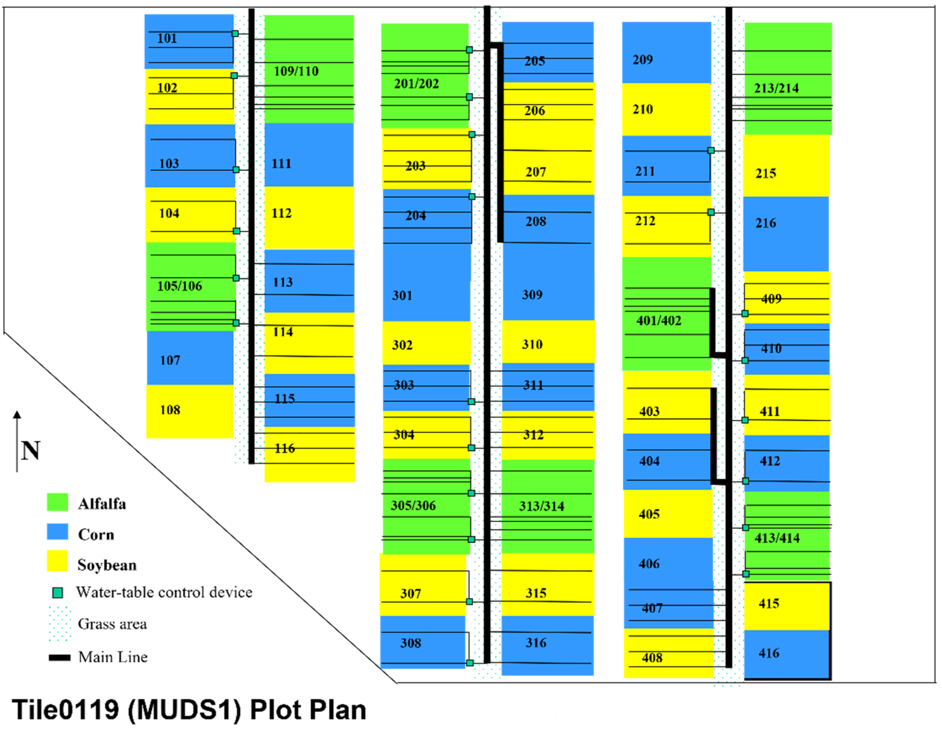
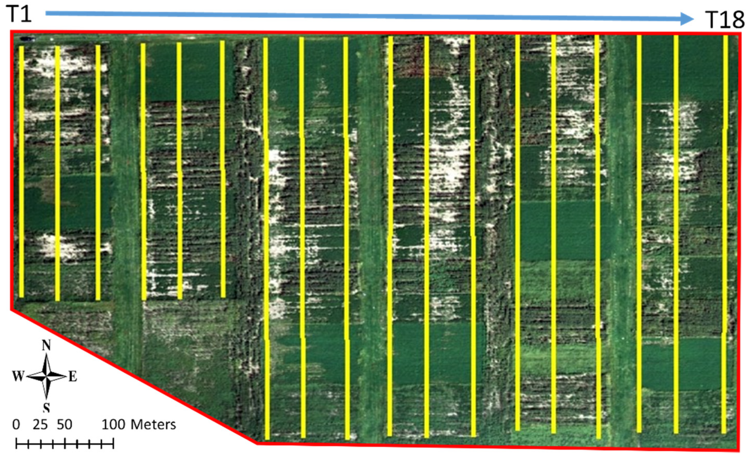
2.1. Study Area

The study area is located at the Greenley agricultural research station in Novelty, MO, USA (Figure 1).
The study area is an 8.9 ha field, and the soil type is primarily silt loam. The soil texture becomes increasingly fine at greater depths from the surface, and the field is underlain by a claypan layer at a depth of 30 to 50 cm below the ground surface. A total of 27 soil samples were collected at nine locations and three depths across the site, and these samples showed similar trends with depth and no significant lateral trends. The topography at the site is minimal. Natural drainage is poor due to the soil texture and flat topography, but tile drains are installed over portions of the site.
The study area is divided into 56 plots with different combinations of crop types and drainage tile configurations. The crops grown at the site are corn (24 plots), soybeans (24 plots), and alfalfa (8 plots). Three drainage tile configurations are used for the corn and soybeans; each plot has either no drainage tiles, drainage tiles separated by 12.2 m, or drainage tiles separated by 6.1 m. The alfalfa plots have drainage tiles installed at irregular intervals. All drainage tiles are installed at a depth of ~60 cm. Figure 2 shows the field site with crop type and drainage tile configuration for each plot; corn, soybean, and alfalfa plots are represented as blue, yellow, or green, respectively. Drainage tile locations are shown using horizontal back lines. The numbers on the plots are used only for record keeping and have no physical significance. Due to the preponderance of corn and soybean plots and the irregularity of drainage tile spacing in alfalfa plots, most of the analyses performed in this research are focused on the corn and soybean plots.

2.2. Vegetation Indices Data Acquisition and Processing

In agriculture, UAV data are normally used to calculate vegetation indices. Different VIs are sensitive to different aspects of vegetative health. A brief description of the VI used in this research is given here.
One of the most commonly used and widely known VI is the Normalized Difference Vegetation Index (NDVI), which is used to evaluate vegetation vigor by estimating the greenness and density of vegetation. One limitation of NDVI data is that they may not be suitable for evaluating vegetation vigor for some crops in the latter portion of their growth period, since very mature vegetation can more easily reach the saturation value of NDVI [45,51,55,57,59,60,61,62,63,64]. However, the Normalized Difference Red Edge Index (NDRE) can often be used under these conditions. NDRE uses a red-edge band instead of the red band in NDVI, and the red-edge band is able to penetrate deeper into the vegetative canopy; NDRE is therefore useful for evaluating permanent or later stage crops, especially for larger plants [45,55,56,59,62,65,66]. Another common vegetation index is the Green Normalized Difference Vegetation Index (GNDVI). It is similar to the NDVI but uses the green and NIR bands to better observe the changes in chlorophyll content in plants, and it is less likely to reach the saturation value than NDVI [45,51,55,62,67]. The Green Chlorophyll Index (CIG) was also selected for this project because it can accurately estimate the total chlorophyll content in leaves and is sensitive to slight changes in leaf chlorophyll content [45,55,62,63,66]. Additionally, CIG is suitable when different types of crops are planted in adjacent plots, which occurs at our study site. The last index used in this study is the Visible Atmospherically Resistant Index (VARI), which is used to estimate vegetation coverage in the image by measuring the reflectance between plants and soil [52,57,62,68]. A lower VARI value indicates very weak vegetation or bare soil. The equation used to calculate each index is given in Table 2.
All the vegetation indices listed are sensitive to and positively correlated with chlorophyll content, and higher chlorophyll content is correlated to greater vegetation vigor. Some indices are normalized for values ranging from −1 to 1, although CIG and VARI are not. Although all indices can be used to indicate areas with stronger or weaker vegetation, there is no quantitative correlation of vegetation indices values with specific crop response, and explanations for the interpretation of these indices may vary. Therefore, vegetation indices are interpreted on a site-specific basis.
The multispectral data used to calculate the vegetation indices at this site were collected on 13 September 2019, using a DJI Inspire 1 V2.0 UAV and a Sentera Double 4 K Lock & Go Sensor. Data were acquired for five spectral bands: blue (446 nm × 60 nm width), green (548 nm × 45 nm width), red (650 nm × 70 nm width), red edge (720 nm × 40 nm width), and near infrared (NIR, 840 nm × 20 nm width). The image overlap was 80%. The crops were fully mature at the time of data acquisition, and no significant precipitation occurred in the two weeks prior to data acquisition.
The multispectral data were processed using Agisoft Metashape software developed by Agisoft LLC. First, the multispectral images were mosaicked to get the orthomosaic map. Then, the raster transform tool was used to calculate the vegetation indices (equations given in Table 2) for each pixel. The vegetation indices data were input into ArcMap (Esri ArcGIS software), which was used to export quantitative values for all indices for each pixel.

2.3. Volumetric Water Content from Ground-Penetrating Radar

GPR is an electromagnetic geophysical method that is used extensively in engineering to image subsurface features. A GPR system consists of a transmitting antenna and a receiving antenna; the transmitter emits high-frequency electromagnetic energy that can be returned to the receiver through reflection, refraction, or as a direct wave between the antennas [69]. This research uses a direct wave, called the groundwave, which travels directly between the antennas in the shallow subsurface. The sampling depth of the groundwave is a function of the antenna frequency, where the sampling depth and frequency are inversely related [70]. The electromagnetic velocity of the shallow subsurface can be determined by measuring the travel time of the groundwave and using the known separation distance between the transmitting and receiving antennas. Detailed descriptions on how the groundwave is used to determine the near-surface electromagnetic velocity is provided by several researchers [15,71,72,73,74].
Once the electromagnetic velocity (v) has been determined, it can be related to the relative dielectric permittivity (εr):
v = c ε r
where c is the velocity of an electromagnetic wave in a vacuum (0.3 m/ns) [75]. The relative dielectric permittivity is primarily influenced by the amount of water in soil pores, as the permittivity of most minerals/soil solids is 3 to 8, while the permittivities of air and water are 1 and 80, respectively [76]. Several petrophysical relationships have been developed to relate the relative dielectric permittivity to a soil’s volumetric water content [12,77,78]. One of the most commonly used relationships is Topp’s equation [79]:
VWC = 5.3 × 10 2 + 2.92 × 10 2 ε r 5.5 × 10 4 ε r 2 + 4.3 × 10 6 ε r 3
This equation was developed using a range of agricultural soils and is commonly applied to agricultural site characterization for point measurements (TDR and capacitance probes), as well as for GPR data.
GPR data were acquired at this site using a PulseEkko Pro System with 500 MHz antennas. For this frequency, the sampling depth was approximately 18 cm [80]. Data were acquired at two different times. For the first data campaign, on 9 July 2019, no precipitation had fallen for approximately three weeks, and the soil was relatively dry. For the second campaign, on 20 July 2019, a 3.9 cm rainfall had occurred the night before data acquisition, and the soil was quite wet. For both campaigns, data were acquired in the common-offset mode, where the transmitting and receiving antennas were kept a constant distance apart. The antenna separation distances for the dry and wet campaigns were 14 cm and 26 cm, respectively. The antenna separation varied between campaigns to allow the most accurate identification of the groundwave when processing GPR data.
GPR data were acquired in 18 traverses across the site (Figure 3). The traverses were separated by 20 m and varied in length from 166 m to 270 m, based on the dimensions of the field. Data were acquired at 10 cm intervals along each traverse.
GPR data were processed using ReflexW software. Data processing was very simple and included only a bandpass filter that was designed using the measured GPR frequencies to remove low- and high-frequency noise. After processing, the groundwave travel time was determined, and the electromagnetic velocity was calculated using the known antenna separation distance. The electromagnetic velocity was converted to the relative dielectric permittivity using Equation (1), and permittivity was used to estimate the volumetric water content using Equation (2). Occasionally, the groundwave was obscured by reflections from a shallow interface or had a weak amplitude and was difficult to identify clearly. If the groundwave was difficult to detect clearly, these measurements were omitted. Additionally, puddles on the ground surface during the wet data acquisition campaign meant that GPR data could not be acquired for a few meters on some traverses. The areas where GPR data could not be acquired are minor, but they result in some differences in the number of measurements between the dry and wet campaigns. For the dry campaign, 41,711 water content measurements were collected, while the wet campaign had 41,480 measurements.

2.4. Electrical Conductivity from Electromagnetic Induction

Electromagnetic induction (EM) is a very mature technology. EM instruments measure the soil EC, which is a measure of how easily electrical current can flow in the subsurface. In agriculture, researchers usually correlate the measured EC with soil texture, soil water content, or soil salinity. For soil texture, higher EC values usually correlate with a greater fraction of fine-grained soil, so EC can be used to map clay content [1,2,3,4,5,81]. Higher EC values also correlate with higher water content; areas with higher water content often have a higher water holding capacity, which is again correlated with soil texture [1,2,3,4,5,12,13,82]. Soil salinity also positively affects EC, so EC has been used to map areas with high salinity [18,19,20]. Since all three of these parameters are important for agricultural management, such as irrigation, fertilization, and crop yield forecasting, EC is a very useful parameter. Additionally, most electromagnetic induction instruments can be used to acquire data quickly (up to a few miles per hour), and the data require minimal processing, so collecting data over large fields is relatively straightforward.
EC measurements were acquired at this site using a Geonics EM38-MK2 conductivity meter. Data were acquired in the horizontal dipole orientation with the transmitting and receiving antenna coils separated by 1 m, and the sampling depth of the measurements was approximately 0.75 m. Data were recorded every 0.1 s, and a high accuracy GPS unit was used to record the location. Measurements were collected along each of the traverses shown in Figure 3. The same data acquisition parameters were used for the wet and dry campaigns.
Data processing for the EC data was minimal, as EC measurements are output directly. Processing was performed to average any duplicate measurements that occurred in one location if the conductivity meter was paused at any point. The measurements acquired for the dry and wet campaigns were 8201 and 9747, respectively.

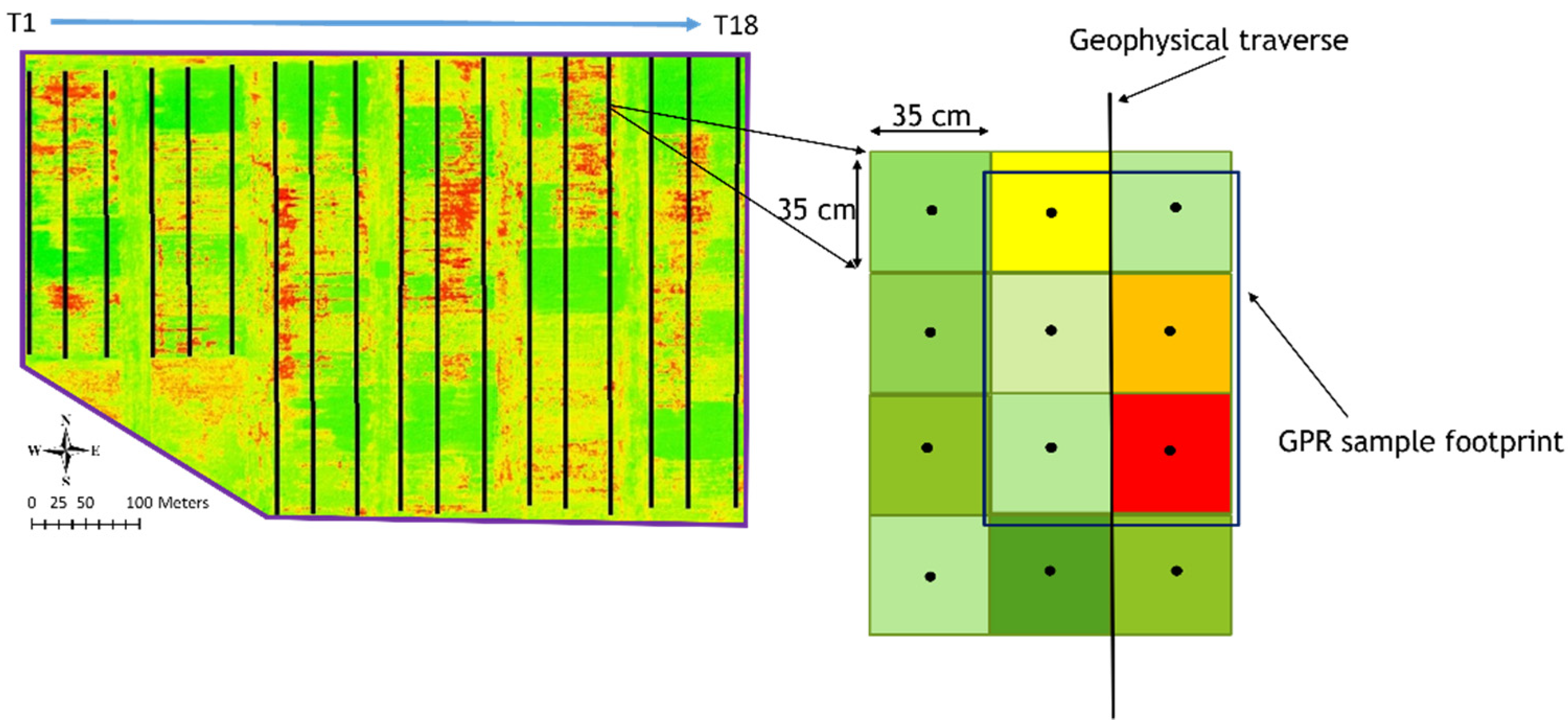
2.5. Resolving Resolution Differences between Multispectral and Geophysical Data

The spatial sampling footprints for geophysical measurements and UAV-based multispectral pixels were different, so processing was required to compare measurements from disparate techniques. The UAV-based data were higher resolution; each pixel had a footprint of 35 cm by 35 cm. For the EC data, the footprint was approximately 1 m wide and 1 m long. For the GPR, the width of the footprint was the antenna width (23 cm), and the length of the footprint was 60 cm and 72 cm for the dry and wet campaigns, respectively. To compare data from multiple data sets, data from different UAV pixels were averaged within the footprint of the geophysical measurements. Averaging was accomplished using the location of the midpoint of each UAV pixel; all UAV measurements with midpoint locations that fell within the footprint of a geophysical measurement were arithmetically averaged for comparison with the geophysical measurement (Figure 4). This process was repeated for all geophysical measurements.

2.6. Machine Learning

Machine learning was performed using the random forest method [83], with VIs and raw band data from the multispectral camera as input. These parameters were used to predict the soil water content and electrical conductivity measured using geophysical techniques. Random forest modeling was chosen because this method is often more interpretable than other types of machine learning, so it will facilitate an understanding of the relationships between VIs and geophysical data. Random forest models also handle outliers well, require less training time than some other machine-learning methods, and can account for non-linear relationships between multiple variables. The random forest method has been used in several studies relating remote-sensing data to soil properties. In one study, researchers estimated soil pH, soil organic matter, and clay content in agricultural fields using the random forest method with Sentinel-2 data [21]. Another study used the random forest method to determine which of several types of satellite-based predictor data were best at estimating the total nitrogen content in topsoil [84]. The random forest method was also used to map the spatial distribution of the organic carbon content in topsoil from satellite-based data [85].
Random forest models use decision trees, each of which predicts a value for the variable of interest, which in this research is the geophysical measurement (VWC or EC). The best estimate for the geophysical measurement is the average estimated value from all the decision trees. Before applying the random forest method, the data were first normalized, so that all variables ranged from 0 to 1. Then, the data were randomly divided into five quintiles. A total of 80% of the data were used for training, and the remaining 20% was used for testing. After the model was run, the mean absolute error (MAE) was calculated for the 20% of data used in the testing, where the MAE was calculated as
MAE = i = 1 n | y i x i | n
In this research, y i is the prediction of VWC or EC; xi is the true value of VWC or EC; and n is the total number of measurements. All calculations (normalization, running the random forest models, and calculating the MAE) were performed using Python.
The modeling process was repeated four additional times, each time using a different quintile for testing, so there are five different tests for each combination of VIs and geophysical data. This method was used to reduce the impact of outliers if any single quintile was not representative of the entire data set. After all five quintiles had been tested, the average MAE for these tests was calculated and used to evaluate each input/output combination.
Some of the hypotheses tested required the removal of a single variable (i.e., one vegetation index) when the model was run. When a variable was removed from the calculations, it was replaced by a “filler” variable consisting of random numbers from 0 to 1, so the total number of variables considered was equal for all models. To determine whether a variable was useful for the prediction of geophysical data, the MAEs that occurred when all data were used were compared to the MAEs that occurred when one variable was omitted. If the MAE was significantly higher when that variable was omitted, it was considered useful for the prediction of geophysical measurements.

3. Results

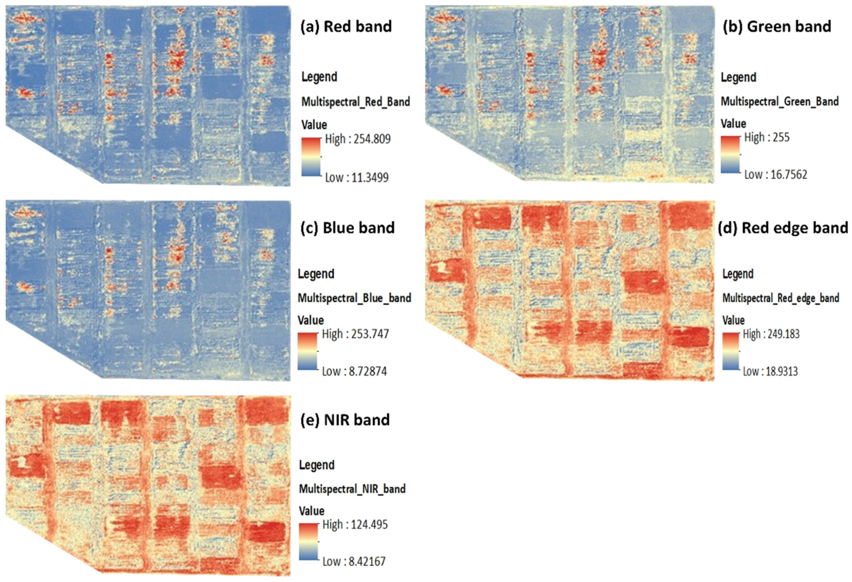
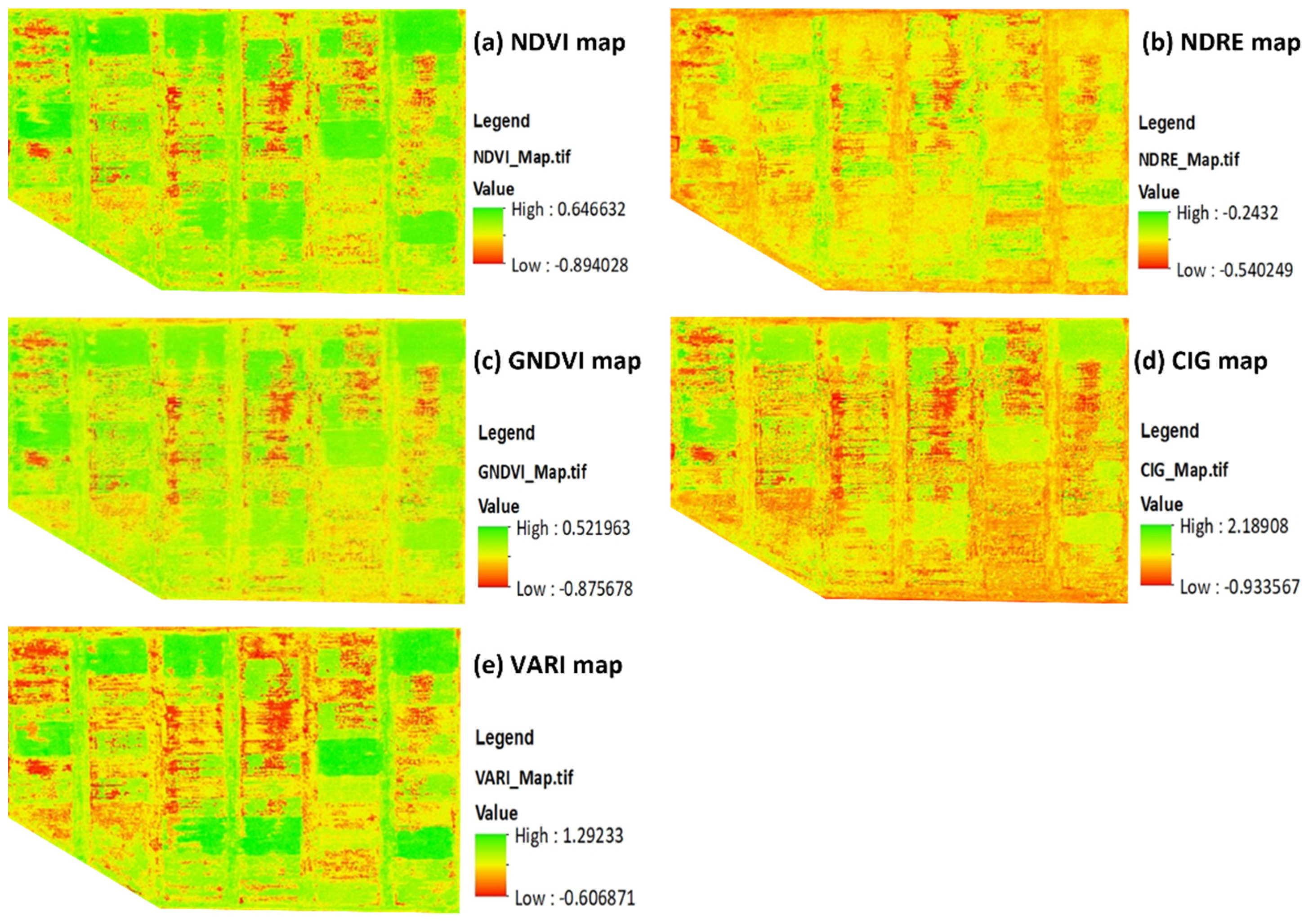
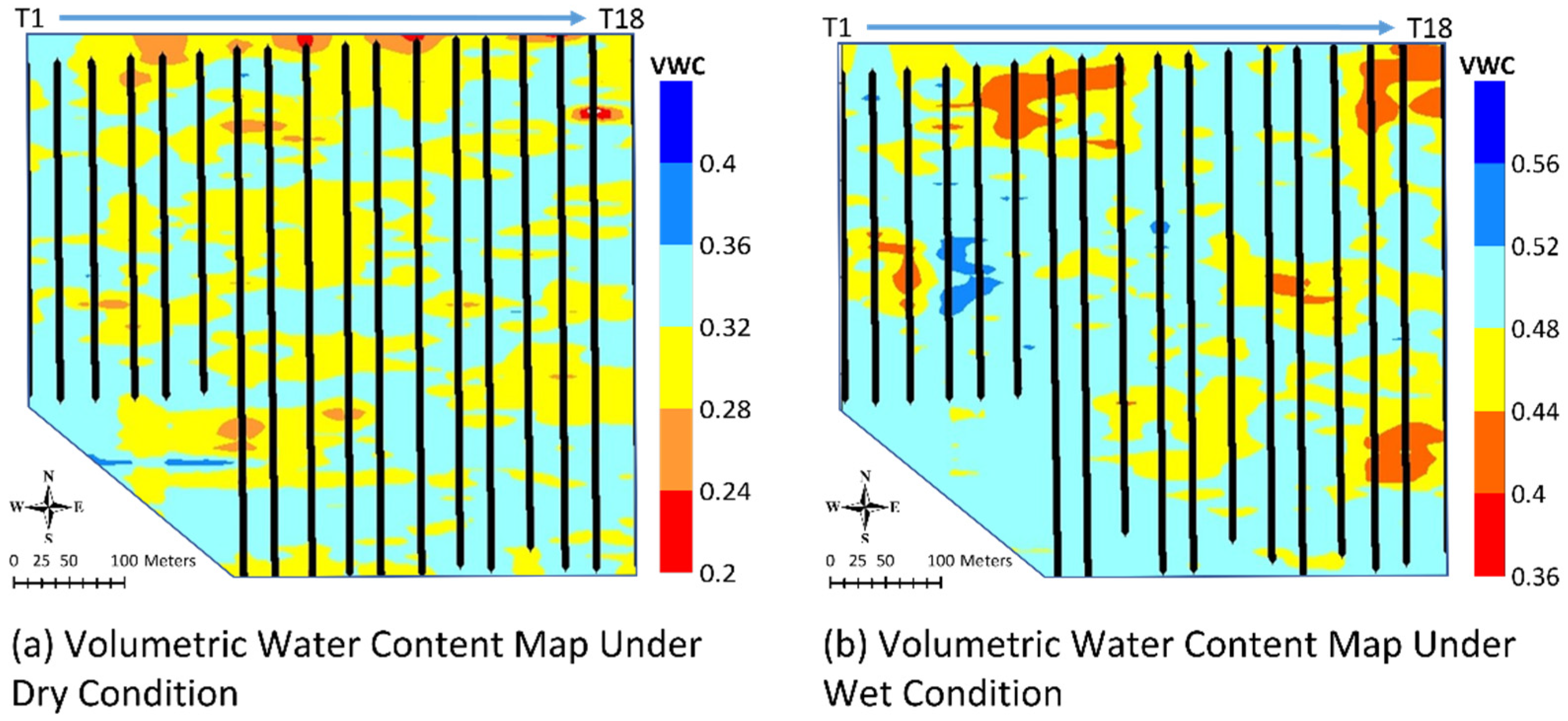
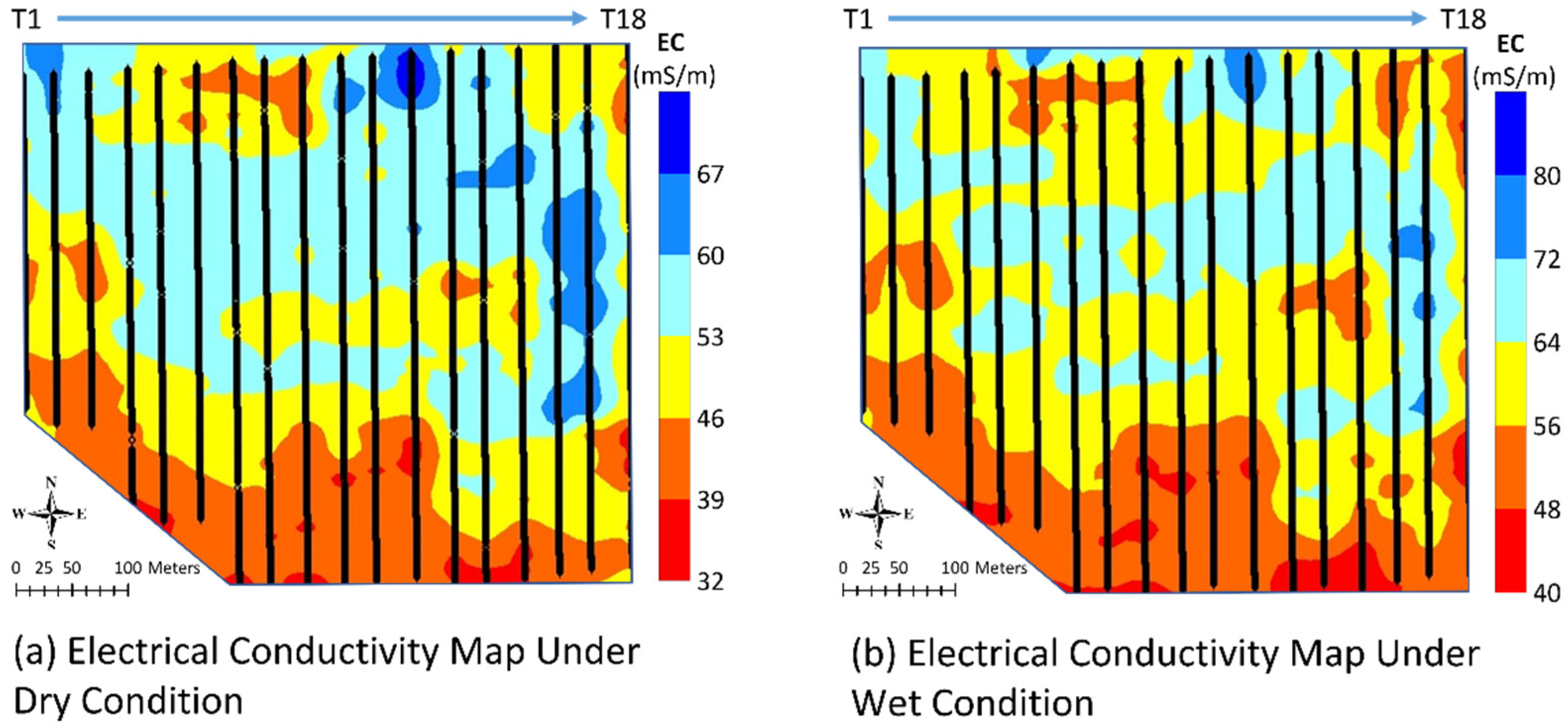
3.1. Maps of Each of the Vegetation Indices, Raw Band Data, Volumetric Water Content (VWC) and Electrical Conductivity (EC)

Figure 5 shows maps of multispectral bands, which are (a) Red band, (b) Green band, (c) Blue band, (d) Red edge band and (e) NIR band. Figure 6 shows maps of the five vegetation indices calculated in this research: (a) NDVI, (b) NDRE, (c) GNDVI, (d) CIG, and (e) VARI. Vegetation indices show significant variations across the field and are strongly influenced by vegetation type. The alfalfa plots are especially noticeable on several of the VIs maps; alfalfa may have higher values for some VIs, since it covers the majority of the ground surface in the alfalfa plots, while corn and soybeans are grown in rows and often have bare patches of soil in between the rows. Similarly, alfalfa is especially noticeable in the maps of the multispectral band data in Figure 5. Indices maps and bands maps are drawn using Agisoft and ArcMap software and show each pixel without interpolation.
Figure 7 and Figure 8 are maps of the VWC and EC, respectively, under dry and wet conditions. These maps were drawn using Surfer, and interpolation was conducted using the nearest neighbor method. (Kriging was tried, but kriging is less successful when data are acquired with closely spaced measurements but widely spaced traverses.) Figure 7 shows that water content varies across the field, and when the soil is very wet, this variability is more pronounced. Figure 8 shows a similar trend for EC.

3.2. Evaluation of Prior Site Knowledge for Estimating Soil Properties Using UAV-Based Multispectral Data

One of the goals of this research was to determine the extent to which prior knowledge of the site, specifically crop type and drainage conditions, affected estimation of soil properties. Four analyses were performed to answer this question. In the first analysis, described in Section 3.2.1, no prior knowledge of the site was assumed, so all data were included, irrespective of crop type or drainage condition. In the second and third analyses, knowledge of either the drainage condition (Section 3.2.2) or crop type (Section 3.2.3) was assumed. In the last analysis (Section 3.2.4), knowledge of both the drainage condition and crop type was assumed.

3.2.1. Prediction of VWC and EC Using All Data, Undifferentiated by Crop Type or Drainage

The data were first analyzed using all the data acquired, regardless of crop type or drainage tile configuration. The purpose of this analysis was to determine how well VIs data could be used to estimate VWC or EC if there was no prior information about the site or if no pre-processing has been performed to separate different sites based on crop type or drainage. Results of this analysis are shown in Table 3; discussion of these results is given in Section 4.1.1.

3.2.2. Prediction of VWC and EC if Only the Drainage Tile Configuration Is Known

This analysis was performed to determine whether more accurate estimates of VWC and EC could be determined from VIs data if the drainage tile configuration of the field was known. For this analysis, the data were sorted based on drainage tile configuration, but not crop type. Because the drainage within the alfalfa plots was irregular, data from these plots were removed from this analysis. Corn and soybean data were then considered together for each of the three drainage tile configurations. Results of this analysis are shown in Table 4; discussion of these results is given in Section 4.1.2.

3.2.3. Prediction of VWC and EC if Only the Crop Type Is Known

The purpose of this analysis was to determine the importance of crop type on the prediction of VWC or EC from VIs data. In this analysis, the data were sorted based on three crop types (corn, soybean, or alfalfa), but drainage tile configuration was not considered. Machine learning was performed separately for each of the three crop types. Results of this analysis are shown in Table 5; discussion of these results is given in Section 4.1.3.

3.2.4. Prediction of VWC and EC if Both the Crop Type and Drainage Configuration Are Known

This analysis was performed to see whether the prediction of VWC and EC could be optimized if both crop type and drainage tile configuration were known. Machine learning was performed separately for each of the three drainage tile configuration data sets for two crop types, corn and soybeans. Plots containing alfalfa were omitted from this analysis because the drainage tile spacing within the alfalfa is irregular. Results of this analysis are shown in Table 6; discussion of these results is given in Section 4.1.4.

3.3. Evaluation of Different UAV-Based Multispectral Data for Estimating Soil Properties

The second major research question in this project was to determine which types of multispectral data were most useful for predicting soil properties. In Section 3.3.1, the importance of different vegetation indices is investigated. In Section 3.3.2, a similar analysis is performed for raw band data.

3.3.1. Evaluation of Individual Vegetation Indices for Predicting VWC and EC

This analysis was performed to determine which VI was the most useful for predicting VWC and EC. To determine this, the MAE was iteratively calculated using all indices except one. If the MAE increased significantly when one index was removed, that index was considered more important for VWC or EC estimation. This analysis was performed for plots separated by drainage tile and crop type and when plots were separated by crop type but not by drainage tile. The only exception was alfalfa, where the plots were not separated by drainage tile configuration because of the irregular tile spacing in the alfalfa.
To summarize the impact of the most important VI, we noted the three VIs which had the most impact (caused the most increase in error when they were removed) each time the analysis was performed. Then, for each crop type and campaign (dry or wet), we summed the number of times each VI was one of the three most important (Table 7). For example, for VWC in corn during the dry campaign, CIG was one of the three most important VIs for no tile drainage, drainage with 12.2 m spacing, and all drainage configurations considered together, so it receives a value of 3 in the table. (The maximum value possible in Table 7 is a 4) Table 7 also records the average increase in MAE that results when each VI was omitted. Discussion of the results shown in Table 7 is given in Section 4.2.1.

3.3.2. Evaluation of Raw Band Data for Predicting VWC and EC

Although most crop evaluations are performed using VIs data, raw band data can also be considered for estimation of VWC and EC. In this analysis, we considered the prediction accuracy of both raw band data and VIs by repeating the analysis described in Section 3.2.2, but this time also including the raw band data. Table 8 can be compared to Table 4 to determine the impact of adding raw band data to the analysis. Additionally, we noted which bands or VIs were most important for prediction following the same process as described in Section 3.3.1 The most important bands or VIs and the error that resulted when these data were removed are noted in Table 8. Discussion of these results is given in Section 4.2.2.

4. Discussion

4.1. Prediction of Soil Properties Using VIs Data

Correlations between VWC and EC and VIs data could be caused by direct causative factors or by indirect correlation between these parameters and soil properties. Vegetation vigor, as measured by VIs, can be directly correlated to VWC when parts of the field are subjected to water stress. Similarly, if parts of the field experience high salinity and have correspondingly high EC, that could also directly impact vegetation vigor and cause a strong correlation between EC and VIs. When water stress or soil salinity are not concerns at a site, vegetation vigor can still be influenced by soil properties. At this site, neither water shortages nor soil salinity are concerns, so correlations between VIs and VWC or EC are most likely to occur because VWC, EC, and vegetation vigor are all influenced by soil properties.

4.1.1. Prediction of VWC and EC Using All Data, Undifferentiated by Crop Type or Drainage

The data shown in Table 3 indicate that the estimation of VWC or EC using machine learning with VIs data is somewhat sensitive to the moisture conditions at the time of the geophysical survey. The estimation of VWC and EC was more accurate (had a lower MAE) when VIs data were correlated to drier data, but this may reflect the lower overall variability in VWC and EC that occurred in the dry soil rather than an improved correlation between VIs and these parameters. If the ratio between the MAE and the standard deviation (σ) is considered, the MAE/σ is somewhat higher for the dry VWC than for the wet VWC, indicating that the improvement in prediction was greater for the wet data. For the EC, MAE/σ is very similar for both wet and dry conditions. The MAE/σ ratio is similar for EC and VWC, indicating that the correlation between these parameters and VIs is also similar. Both VWC and EC are influenced by soil texture, which can also influence VIs values; it is likely that soil texture contributes strongly to correlations between these parameters.

4.1.2. Prediction of VWC and EC if Only the Drainage Tile Configuration Is Known

Comparison of the results in Table 3 and Table 4 shows that for both VWC and EC, VIs data more accurately predict these parameters when the data are separated by drainage tile configuration than when the configuration is unknown. For both VWC and EC data, parameter prediction does not appear to be affected by the specific drainage configuration (i.e., predictions in plots with no drainage are not notably more accurate than in plots with high drainage), and similar MAE/σ ratios are observed in the VWC and EC data for most drainage configurations for both wet and dry soils. These results suggest that, although sorting based on tile configuration can improve estimation of VWC and EC, there is no obvious improvement in estimation based upon the degree of drainage in a field.

4.1.3. Prediction of VWC and EC if Only the Crop Type Is Known

Comparison of Table 3 and Table 5 shows that for both wet and dry VWC, the MAE is less when crop types are considered separately for corn and soybeans, but the MAE in alfalfa increases when the alfalfa is considered separately. This trend reflects changes in variability when the crop types are considered separately; the VWC σ of the corn and soybeans decreases when crops are considered separately, but the σ of the alfalfa increases. The higher variability of VWC in alfalfa may reflect the irregular tile drainage configuration in the alfalfa, but it may also be caused by the state of maturity of the alfalfa plants at the time of GPR data acquisition; the alfalfa plants were larger and more mature than the corn or soybean plants, and therefore were probably extracting water more differentially through their root systems. Additionally, alfalfa plants did not grow in rows like the corn and soybeans, so they covered more of the ground surface. Although the overall MAE in the alfalfa is higher when it is considered separately, the MAE/σ of VWC is considerably less than when all crops are considered together, while this ratio remains about the same or increases slightly for the corn and soybeans. Thus, separating plots based on crop type overall results in a more accurate estimation of VWC from VIs data for all crop types. Predictions of EC from VIs data are somewhat different from those of VWC after the impact of crop type is considered. Separating out corn crops makes little difference in predicting EC; the MAE and the MAE/σ are slightly higher than for dry data or the same as for wet data for just corn when compared to all crops considered together. For soybeans, these parameters are lower when soybeans are considered separately, and they are considerably lower when alfalfa is considered separately. This improved prediction seems to largely be a function of the lower EC variability with each crop type, as the MAE/σ is higher for each of the separated crop types than when all crops are considered together. This is especially notable for alfalfa, which had a significantly lower MAE/σ ratio for VWC, but not for EC; for EC, all crop types have similar MAE/σ ratios, which are also similar to these ratios for VWC in corn and soybeans.
EC is also different from VWC, in that there is a notable difference between wet and dry EC predictions. For VWC, the variability and the MAE are similar for dry and wet conditions. For EC data, drier conditions have less variability and lower MAE, although the MAE/σ ratio is slightly higher for the dry soil. A possible explanation for the greater variability of the EC data when the soil is wet may be the response of the mostly clay soil to additional moisture. As the pores fill with water, some of the clay minerals also start to expand, which causes greater connectivity between grains and can increase bulk EC. The higher EC variability observed during the wet campaign may therefore be caused by changes in both the pore water content and the connectivity of the soil matrix.

4.1.4. Prediction of VWC and EC if Both the Crop Type and Drainage Configuration Are Known

Comparison of Table 3 and Table 6 shows that separating out crop type and drainage configuration reduces the σ of VWC for both wet and dry data. Unsurprisingly, the MAE is also reduced. However, the MAE/σ is also lower for the separated data, indicating that the improvement in prediction is not solely due to the reduction in variability and that separating plots based on crop type and drainage tile configuration will provide the most accurate VWC estimates. For EC, the MAE is lower when the plots are considered separately, but the variability is not always reduced compared to the combined data sets, especially for the dry data.
Comparison of Table 4 and Table 6 was performed to see whether VWC and EC could be better predicted by separating plots based on both crop type and drainage than could be done by separating only based on drainage. Analysis of these data shows that crop type is an important variable; Table 6 shows that the MAE in corn is considerably higher than in soybeans for both the wet and dry VWC and EC. Comparison of Table 4 and Table 6 shows that the MAEs in corn plots separated by drainage tile are usually greater than or the same as corn+soybean plots separated by drainage tile when the soil is dry, while the MAE in soybeans is less than the corn+soybean plots separated by drainage tile for both dry and wet soils. Separating out by crop type and drainage tile overall produces better estimates (lower MAE/σ ratios) than keeping crop types together, but because of the disparity in prediction in corn and soybeans, the MAE does not always decrease in corn when the plots are separated by crop type.
Comparison of Table 5 and Table 6 was performed to see whether VWC and EC could be better predicted by separating plots based on both crop type and drainage than could be done by separating only based on crop type. Analysis of data in these tables shows that separating crops by drainage after first sorting by crop type improves both VWC and EC estimates, although the improvement was somewhat more notable in the VWC than in the EC.

4.2. Evaluation of Different Multispectral Data for Estimating Soil Properties

Different bands of multispectral data respond to different aspects of vegetation vigor or soil properties. VIs, which are calculated using different combinations of these bands, are similarly dependent upon vegetative and soil characteristics. Section 4.2.1 discusses why different VIs may correlate with VWC and EC, while Section 4.2.2 provides a similar discussion for raw band data.

4.2.1. Evaluation of Individual Vegetation Indices for Predicting VWC and EC

Analysis of Table 7 shows that for both VWC and EC and for all three crops, the three indices that have the most impact on estimation are usually NDRE, VARI, and CIG, although NDVI and GNDVI appear occasionally. Possible explanations for why these indices are important are discussed below.
The NDRE is calculated using NIR and red-edge instead of visible bands. The red-edge band is able to penetrate deeper into the canopy than visible bands, so this index is often effective for crops in the later stages of growth. The VIs data for this experiment were collected when the three crops were in the later stages of growth, especially for the corn, where the top leaves and tassels had begun to turn yellow and withered. The deeper penetration of the NDRE was able to obtain information from the healthier leaves in the lower layer that better represented the vigor of the entire plant. For alfalfa and soybeans, most of the leaves remained green at all levels, so the NDRE data also captured this information. Vegetation vigor is related to VWC and EC, so the better representation of vigor observed in the NDRE data was useful for VI prediction.
The VARI was the second most important VI for predicting VWC and EC. VARI is calculated using three visible bands (green, red, and blue), and it is often useful in determining areas with vegetation instead of bare soil. There were frequent patches of bare soil in the experimental area; since vegetation typically changes the VWC (and thus the EC of soil), it is likely that these bare patches differed in VWC and EC compared to areas with vegetation. Thus, the identification of these areas helps to predict these parameters.
The third most important VI in this experiment was CIG, which is calculated using NIR and the green band. CIG is directly proportional to the NIR and inversely proportional to the green band. The importance of CIG to this analysis is probably due to the influence of the green band, which is highly sensitive to the amount of chlorophyll [63]. The green band is thus closely related to plant vigor, but it does not penetrate as far into the canopy as red edge, so CIG may reflect the vigor of the leaves near the surface of the canopy. Although this analysis showed that measurements that penetrated deeper into the canopy (NDRE) were more correlated to the soil properties, the prominence of CIG data in the results indicated that shallower canopy measurements can also be correlated to soil properties.
Although the results are not included in this study, simple linear correlation was also performed between VIs and VWC or EC data. The regression coefficients for these relationships were generally too low (usually R2 < 0.1) for individual VI to be used for VWC or EC prediction; multi-variate machine learning was much more successful. However, the simple linear correlation results can be compared to the evaluation of the importance of individual VI in machine learning. The two VIs that had the highest regression coefficients when simple linear correlations were calculated were VARI and NDRE. These VIs were also the most important predictors for machine learning, as discussed above. The VI that had the third best simple linear correlation with VWC or EC data was NDVI. This is slightly different from what was observed in the machine-learning results, where CIG was the third most significant VI. This indicates that CIG is useful for prediction in conjunction with other types of data but may be less useful by itself.

4.2.2. Evaluation of Raw Band Data for Predicting VWC and EC

Comparison of the MAE in Table 4 and Table 8 shows that for both VWC and EC data, under both wet and dry conditions, inclusion of the raw band data significantly reduces the MAE and the MAE/σ ratio for all drainage configurations. This shows that the estimation of these parameters can be improved when raw data (band values) are included in the machine-learning process.
Comparison of Table 7 and Table 8 shows that, while VIs are still important for estimation, the raw band data are also important. For VWC, the blue band, VARI, and NDRE have the most impact on MAE. For EC, the blue band is the most important parameter, followed by the red band, VARI, and CIG. The importance of the blue band compared to the VIs was unexpected but may be partially due to the lack of blue band input into most VIs. Table 2 shows that of the VIs used in this study, only VARI use blue band as input. Therefore, if the blue band is correlated to VWC or EC, this correlation is less likely to be discovered through a VI. The blue band is correlated primarily with the health of vegetation [86], which is probably correlated with soil texture, and thus with EC and VWC. The same is true for red band data, although, at this site, the blue band appears more important, since blue appeared more than twice as often as red in the top three correlations for EC and VWC.

5. Conclusions

This research investigated using UAV multispectral data and machine learning to predict VWC and EC, which were acquired using geophysical methods. The prediction of VWC and EC was investigated as a function of crop type and drainage tile configuration, as well as by the data input (different VIs and raw band data). Results showed that VIs data can help with the prediction of VWC and EC, and that the most accurate results for these parameters were obtained when both the crop type and drainage tile configuration were known. If limited information was known about a field, VIs data still improved the estimation if either crop type or drainage tile configuration was known; knowledge of the drainage tile configuration resulted in more improvement than knowledge of the crop type at this site.
For VWC, the prediction was better in drier soil than in wet soil if the drainage tile configuration was unknown. If the drainage tile configuration was known, the prediction of VWC was similar for dry and wet soils. For EC, the prediction was generally better in dry soil than in wet soil. These trends probably reflect the overall variability during drier and wetter times, but they do indicate that prediction will be more difficult in wetter soils.
Analysis of the contributions of different VIs and raw band data to the prediction of VWC and EC shows that VIs that penetrate more deeply into the canopy (NDRE) and that are sensitive to bare soil (VARI) were most important. Raw band data, especially the blue band, improved the prediction of VWC and EC. This implies that raw band data, which are often not analyzed by producers, should be included in future analyses.
One factor that probably reduces the accuracy of predictions of VWC and EC from UAV data for this study is that the data collection for the geophysical data and the VIs data was performed on different days. This was unavoidable for this study, as the geophysical data had to be acquired while the crops were small enough to move the geophysical equipment between plants, but the UAV data were acquired when the crops were mature. UAV data acquisition was performed at this later date to better mimic data collected by producers and to better distinguish different crops, as VIs data on very immature crops is less useful. Our results show that UAV data were helpful for improving the predictions of VWC and EC, but the improvements might have been greater if geophysical and UAV data were able to be acquired at the same time.
Although the time lapse between data acquisition with geophysical methods and multispectral data may reduce the accuracy of the estimated VWC and EC somewhat, we feel that this time lapse does not impact the overall validity of our results. First, the relationships between soil properties and multispectral data that were found with machine learning are not primarily based on the direct response of the multispectral data to bare soil. Instead, the multispectral data are mostly sensitive to vegetation vigor. While vegetation vigor is related to soil VWC and EC, it is an averaged response to these soil properties over time. Thus, the vegetation vigor can be better understood to correlate to the average VWC or EC in the field. In this research, multispectral data were found to be useful for estimating VWC and EC at two different times (with both wetter and dryer soil), showing that the patterns of VWC and EC are somewhat continuous with time. This is also shown in Figure 7 and Figure 8, which show similar distributions under wet and dry times; this pattern is what would be expected if VWC and EC were strongly influenced by soil texture, which does not change with time. Thus, it is likely that the correlations between VWC and EC data and multispectral data are indicative of correlations between soil texture and multispectral data/vegetation vigor, and the temporal stability of soil texture reduces the importance of the timing of geophysical data acquisition. Additionally, other researchers have observed strong correlations between remotely sensed data and ground-based measurements that were acquired at different times. The authors of reference [2] observed that Landsat-5 imagery had a strong correlation with soil EC acquired three years prior to the satellite measurements. The authors of reference [24] successfully correlated Sentinel-2 data with soil samples of clay and organic matter that were acquired one to two months later than the satellite data. The authors of [85] related multispectral data acquired from Landsat imagery with soil carbon that was acquired two years after the Landsat imagery. These studies show that if some underlying soil properties are constant, remote-sensing imagery can be correlated to ground-based measurements acquired at a different time.
Another reason that we feel our results are valid is the rigor of the machine-learning process. Our data set was robust, and we observed machine learning to make sure enough data points were provided for training to occur successfully. To ensure that outliers did not influence our results, we randomly divided the data into five quintiles and ran the machine-learning algorithm five times for each set of predictors and output, each time reserving a different quintile for testing of the developed relationships. The MAE values shown in the results are the averages of the five MAE values calculated for the five quintiles. Thus, we feel that the machine-learning procedure we followed was suitably rigorous and that the resulting correlations are credible.
The correlation of ground-based geophysical data with UAV data is a new field, and much further work is needed. Studies with no time lapse between data acquisition of different techniques are needed, as are studies using different crops, soil textures, and geophysical methods. Finally, other types of machine learning could be employed to determine which techniques are optimal for this application.

Author Contributions

Conceptualization, Y.G. and K.G.; methodology, Y.G. and K.G.; software, J.S.; formal analysis, Y.G.; investigation, Y.G., K.G. and K.L.; resources, K.G.; data curation, J.S.; writing—original draft preparation, Y.G.; writing—review and editing, K.G.; supervision, K.G.; project administration, K.G. All authors have read and agreed to the published version of the manuscript.

Funding

This research received no external funding.

Data Availability Statement

Not applicable.

Acknowledgments

Our sincere gratitude is extended to Kelly Nelson, who provided site access, maps, and invaluable site guidance.

Conflicts of Interest

The authors declare no conflict of interest.

References

  1. Corwin, D.; Lesch, S. Application of Soil Electrical Conductivity to Precision Agriculture. Agron. J. 2003, 95, 455–471. [Google Scholar] [CrossRef]
  2. Guo, W.; Maas, S.; Bronson, K. Relationship between cotton yield and soil electrical conductivity, topography, and Landsat imagery. Precis. Agric. 2012, 13, 678–692. [Google Scholar] [CrossRef]
  3. Wiatrak, P.; Khalilian, A.; Mueller, J.; Henderson, W. Applications of Soil Electrical Conductivity In Production Agriculture. Better Crops 2009, 93, 16–17. [Google Scholar]
  4. Robinson, D.; Lebron, I.; Kocar, B.; Phan, K.; Sampson, M.; Crook, N.; Fendorf, S. Time-lapse geophysical imaging of soil moisture dynamics in tropical deltaic soils: An aid to interpreting hydrological and geochemical processes. Water Resour. Res. 2009, 45. [Google Scholar] [CrossRef]
  5. Stadler, A.; Rudolph, S.; Kupisch, M.; Langensiepen, M.; van der Kruk, J.; Ewert, F. Quantifying the effects of soil variability on crop growth using apparent soil electrical conductivity measurements. Eur. J. Agron. 2015, 64, 8–20. [Google Scholar] [CrossRef]
  6. Bittelli, M. Measuring Soil Water Content: A Review. HortTechnology 2011, 21, 293–300. [Google Scholar] [CrossRef]
  7. Chan, D.; Rajeev, P.; Gallage, C.; Kodikara, J. Taiwan Ge-Otechnical Society/Southeast Asian Geotechnical Society. In Proceedings of the Seventeenth Southeast Asian Geotechnical Conference, Taipei, Taiwan, 10–13 May 2010; pp. 92–95. [Google Scholar]
  8. Evett, S.; Parkin, G. Advances in Soil Water Content Sensing: The Continuing Maturation of Technology and Theory. Vadose Zone J. 2005, 4, 986–991. [Google Scholar] [CrossRef]
  9. Gardner, C.; Dean, T.; Cooper, J. Soil Water Content Measurement with a High-Frequency Capacitance Sensor. J. Agric. Eng. Res. 1998, 71, 395–403. [Google Scholar] [CrossRef]
  10. Huisman, J.; Sperl, C.; Bouten, W.; Verstraten, J. Soil water content measurements at different scales: Accuracy of time domain reflectometry and ground-penetrating radar. J. Hydrol. 2001, 245, 48–58. [Google Scholar] [CrossRef]
  11. Piikki, K.; Söderström, M.; Wetterlind, J.; Stenberg, B. Digital Soil Mapping for Modelling of Transport Pathways for Pesticides to Surface Water; Swedish University of Agricultural Sciences: Uppsala, Sweden, 2015. [Google Scholar]
  12. Robinson, D.; Gardner, C.; Cooper, J. Measurement of relative permittivity in sandy soils using TDR, capacitance and theta probes: Comparison, including the effects of bulk soil electrical conductivity. J. Hydrol. 1999, 223, 198–211. [Google Scholar] [CrossRef]
  13. Robinson, D.; Jones, S.; Wraith, J.; Or, D.; Friedman, S. A review of advances in dielectric and electrical conductivity measurement in soils using time domain reflectometry. Vadose Zone J. 2003, 2, 444. [Google Scholar] [CrossRef]
  14. Walker, J.; Willgoose, G.; Kalma, J. In Situ Measurement of Soil Moisture: A Comparison of Techniques. J. Hydrol. 2004, 293, 85–99. [Google Scholar] [CrossRef]
  15. Huisman, J.; Hubbard, S.; Redman, J.; Annan, A. Measuring Soil Water Content with Ground Penetrating Radar: A Review. Vadose Zone J. 2003, 2, 476–491. [Google Scholar] [CrossRef]
  16. Klotzsche, A.; Jonard, F.; Looms, M.; van der Kruk, J.; Huisman, J. Measuring Soil Water Content with Ground Penetrating Radar: A Decade of Progress. Vadose Zone J. 2018, 17, 180052–180059. [Google Scholar] [CrossRef] [Green Version]
  17. Zajícová, K.; Chuman, T. Application of ground penetrating radar methods in soil studies: A review. Geoderma 2019, 343, 116–129. [Google Scholar] [CrossRef]
  18. Corwin, D.; Lesch, S.; Shouse, P.; Soppe, R.; Ayars, J. Identifying Soil Properties That Influence Cotton Yield Using Soil Sampling Directed by Apparent Soil Electrical Conductivity. Agron. J. 2003, 95, 352. [Google Scholar] [CrossRef] [Green Version]
  19. Corwin, D.; Lesch, S. Apparent soil electrical conductivity measurements in agriculture. Comput. Electron. Agric. 2005, 46, 11–43. [Google Scholar] [CrossRef]
  20. Lech, M.; Fronczyk, J.; Radziemska, M.; Podlasek, A.; Kazimierz, G.; Koda, E.; Lechowicz, Z. Monitoring of Total Dissolved Solids on Agricultural Lands Using Electrical Conductivity Measurements. Appl. Ecol. Environ. Res. 2016, 14, 285–295. [Google Scholar] [CrossRef]
  21. Yuzugullu, O.; Lorenz, F.; Fröhlich, P.; Liebisch, F. Understanding Fields by Remote Sensing: Soil Zoning and Property Mapping. Remote Sens. 2020, 12, 1116. [Google Scholar] [CrossRef] [Green Version]
  22. Vaudour, E.; Gomez, C.; Fouad, Y.; Lagacherie, P. Sentinel-2 image capacities to predict common topsoil properties of temperate and Mediterranean agroecosystems. Remote Sens. Environ. 2019, 223, 21–33. [Google Scholar] [CrossRef]
  23. Castaldi, F.; Chabrillat, S.; Van Wesemael, B. Sampling Strategies for Soil Property Mapping Using Multispectral Sentinel-2 and Hyperspectral EnMAP Satellite Data. Remote Sens. 2019, 11, 309. [Google Scholar] [CrossRef] [Green Version]
  24. Santaga, F.S.; Agnelli, A.; Leccese, A.; Vizzari, M. Using Sentinel-2 for Simplifying Soil Sampling and Mapping: Two Case Studies in Umbria, Italy. Remote Sens. 2021, 13, 3379. [Google Scholar] [CrossRef]
  25. Ramos, T.B.; Castanheira, N.; Oliveira, A.R.; Paz, A.M.; Darouich, H.; Simionesei, L.; Farzamian, M.; Gonçalves, M.C. Soil salinity assessment using vegetation indices derived from Sentinel-2 multispectral data. application to Lezíria Grande, Portugal. Agric. Water Manag. 2020, 241, 106387. [Google Scholar] [CrossRef]
  26. Zribi, M.; Nativel, S.; Le Page, M. Analysis of Agronomic Drought in a Highly Anthropogenic Context Based on Satellite Monitoring of Vegetation and Soil Moisture. Remote Sens. 2021, 13, 2698. [Google Scholar] [CrossRef]
  27. Yang, Y.; Zhang, J.; Bao, Z.; Ao, T.; Wang, G.; Wu, H.; Wang, J. Evaluation of Multi-Source Soil Moisture Datasets over Central and Eastern Agricultural Area of China Using in Situ Monitoring Network. Remote Sens. 2021, 13, 1175. [Google Scholar] [CrossRef]
  28. Jia, Y.; Jin, S.; Savi, P.; Yan, Q.; Li, W. Modeling and Theoretical Analysis of GNSS-R Soil Moisture Retrieval Based on the Random Forest and Support Vector Machine Learning Approach. Remote Sens. 2020, 12, 3679. [Google Scholar] [CrossRef]
  29. Han, L.; Wang, C.; Yu, T.; Gu, X.; Liu, Q. High-Precision Soil Moisture Mapping Based on Multi-Model Coupling and Background Knowledge, Over Vegetated Areas using Chinese GF-3 and GF-1 Satellite Data. Remote Sens. 2020, 12, 2123. [Google Scholar] [CrossRef]
  30. Babaeian, E.; Sadeghi, M.; Jones, S.; Montzka, C.; Vereecken, H.; Tuller, M. Ground, Proximal, and Satellite Remote Sensing of Soil Moisture. Rev. Geophys. 2019, 57, 530–616. [Google Scholar] [CrossRef] [Green Version]
  31. Gangat, R.; van Deventer, H.; Naidoo, L.; Adam, E. Estimating Soil Moisture Using Sentinel-1 and Sentinel-2 Sensors for Dryland and Palustrine Wetland Areas. S. Afr. J. Sci. 2020, 116, 1–9. [Google Scholar] [CrossRef]
  32. Liu, Y.; Qian, J.; Yue, H. Comprehensive Evaluation of Sentinel-2 Red Edge and Shortwave-Infrared Bands to Estimate Soil Moisture. IEEE J. Sel. Top. Appl. Earth Obs. Remote Sens. 2021, 14, 7448–7465. [Google Scholar] [CrossRef]
  33. Phiri, D.; Simwanda, M.; Salekin, S.; Nyirenda, V.R.; Murayama, Y.; Ranagalage, M. Sentinel-2 Data for Land Cover/Use Mapping: A Review. Remote Sens. 2020, 12, 2291. [Google Scholar] [CrossRef]
  34. Sentinel-2—Missions—Sentinel Online. Available online: https://sentinel.esa.int/web/sentinel/missions/sentinel-2 (accessed on 11 June 2021).
  35. Sentinel 2—Bands and Combinations—GIS Geography. Available online: https://gisgeography.com/sentinel-2-bands-combinations/ (accessed on 11 January 2021).
  36. Aboutalebi, M.; Allen, L.N.; Torres-Rua, A.F.; McKee, M.; Coopmans, C. Estimation of soil moisture at different soil levels using machine learning techniques and unmanned aerial vehicle (UAV) multispectral imagery. In Autonomous Air and Ground Sensing Systems for Agricultural Optimization and Phenotyping IV; Thomasson, J.A., McKee, M., Moorhead, R.J., Eds.; SPIE: Baltimore, MD, USA, 2019; Volume 11008, pp. 216–226. [Google Scholar] [CrossRef] [Green Version]
  37. Allred, B.; Eash, N.; Freeland, R.; Martinez, L.; Wishart, D. Effective and efficient agricultural drainage pipe mapping with UAS thermal infrared imagery: A case study. Agric. Water Manag. 2018, 197, 132–137. [Google Scholar] [CrossRef]
  38. Allred, B.; Martinez, L.; Fessehazion, M.; Rouse, G.; Williamson, T.; Wishart, D.; Koganti, T.; Freeland, R.; Eash, N.; Batschelet, A.; et al. Overall results and key findings on the use of UAV visible-color, multispectral, and thermal infrared imagery to map agricultural drainage pipes. Agric. Water Manag. 2020, 232, 106036. [Google Scholar] [CrossRef]
  39. Freeland, R.; Allred, B.; Eash, N.; Martinez, L.; Wishart, D. Agricultural drainage tile surveying using an unmanned aircraft vehicle paired with Real-Time Kinematic positioning—A case study. Comput. Electron. Agric. 2019, 165, 104946. [Google Scholar] [CrossRef]
  40. Ge, X.; Wang, J.; Ding, J.; Cao, X.; Zhang, Z.; Liu, J.; Li, X. Combining UAV-based hyperspectral imagery and machine learning algorithms for soil moisture content monitoring. PeerJ 2019, 7, e6926. [Google Scholar] [CrossRef]
  41. Gu, H.; Lin, Z.; Guo, W.; Deb, S. Retrieving Surface Soil Water Content Using a Soil Texture Adjusted Vegetation Index and Unmanned Aerial System Images. Remote Sens. 2021, 13, 145. [Google Scholar] [CrossRef]
  42. Hassan-Esfahani, L.; Torres-Rua, A.; Jensen, A.; McKee, M. Assessment of Surface Soil Moisture Using High-Resolution Mul-ti-Spectral Imagery and Artificial Neural Networks. Remote Sens. 2015, 7, 2627–2646. [Google Scholar] [CrossRef] [Green Version]
  43. Sona, G.; Passoni, D.; Pinto, L.; Pagliari, D.; Masseroni, D.; Ortuani, B.; Facchi, A. UAV Multispectral Survey to Map Soil and Crop for Precision Farming Applications; International Society for Photogrammetry and Remote Sensing (ISPRS): Nice, France, 2016; Volume XLI-B1, pp. 1023–1029. [Google Scholar]
  44. Williamson, T.; Dobrowolski, E.; Meyer, S.; Frey, J.; Allred, B. Delineation of Tile-Drain Networks Using Thermal and Mul-tispectral Imagery—Implications for Water Quantity and Quality Differences from Paired Edge-of-Field Sites. J. Soil Water Conserv. 2018, 74, 1–11. [Google Scholar] [CrossRef] [Green Version]
  45. Yeom, J.; Jung, J.; Chang, A.; Ashapure, A.; Maeda, M.; Maeda, A.; Landivar, J. Comparison of Vegetation Indices Derived from UAV Data for Differentiation of Tillage Effects in Agriculture. Remote Sens. 2019, 11, 1548. [Google Scholar] [CrossRef] [Green Version]
  46. Zhang, C.; Kovacs, J. The application of small unmanned aerial systems for precision agriculture: A review. Precis. Agric. 2012, 13, 693–712. [Google Scholar] [CrossRef]
  47. Daponte, P.; Vito, L.D.; Glielmo, L.; Iannelli, L.; Liuzza, D.; Picariello, F.; Silano, G. A Review on the Use of Drones for Precision Agriculture. IOP Conf. Ser. Earth Environ. Sci. 2019, 275, 012022. [Google Scholar] [CrossRef]
  48. Delgado Vera, C.; Aguirre Munizaga, M.; Jiménez, M.; Manobanda, N.; Rodríguez-Méndez, A. A Photogrammetry Software as a Tool for Precision Agriculture: A Case Study; Springer: Cham, Switzerland, 2017; pp. 282–295. [Google Scholar] [CrossRef]
  49. Govorcin, M.; Pribicevic, B.; Đapo, A. Comparison and Analysis of Software Solutions for Creation of a Digital Terrain Model Using Unmanned Aerial Vehicles. In Proceedings of the 14th International Multidisciplinary Scientific Geo-Conference and Expo 2014 (SGEM 2014), Albena, Bulgaria, 17–26 June 2014; Volume 3. [Google Scholar]
  50. Ziliani, M.; Parkes, S.; Hoteit, I.; McCabe, M. Intra-Season Crop Height Variability at Commercial Farm Scales Using a Fixed-Wing UAV. Remote Sens. 2018, 10, 2007. [Google Scholar] [CrossRef] [Green Version]
  51. Candiago, S.; Remondino, F.; De Giglio, M.; Dubbini, M.; Gattelli, M. Evaluating Multispectral Images and Vegetation Indices for Precision Farming Applications from UAV Images. Remote Sens. 2015, 7, 4026–4047. [Google Scholar] [CrossRef] [Green Version]
  52. Li, S.; Yuan, F.; Ata-Ui-Karim, S.; Zheng, H.; Cheng, T.; Liu, X.; Tian, Y.; Zhu, Y.; Cao, W.; Cao, Q. Combining Color Indices and Textures of UAV-Based Digital Imagery for Rice LAI Estimation. Remote Sens. 2019, 11, 1763. [Google Scholar] [CrossRef] [Green Version]
  53. Turner, D.; Lucieer, A.; Watson, C. Development of an Unmanned Aerial Vehicle (UAV) for hyper resolution vineyard mapping based on visible, multispectral, and thermal imagery. In Proceedings of the 34th International Symposium on Remote Sensing of Environment, Sydney, Australia, 10–15 April 2011. [Google Scholar]
  54. Zheng, H.; Cheng, T.; Li, D.; Zhou, X.; Yao, X.; Tian, Y.; Cao, W.; Zhu, Y. Evaluation of RGB, Color-Infrared and Multispectral Images Acquired from Unmanned Aerial Systems for the Estimation of Nitrogen Accumulation in Rice. Remote Sens. 2018, 10, 824. [Google Scholar] [CrossRef] [Green Version]
  55. Ramos, A.P.M.; Osco, L.P.; Furuya, D.E.G.; Gonçalves, W.N.; Santana, D.C.; Teodoro, L.P.R.; da Silva Junior, C.A.; Capristo-Silva, G.F.; Li, J.; Baio, F.H.R.; et al. A Random Forest Ranking Approach to Predict Yield in Maize with UAV-Based Vegetation Spectral Indices. Comput. Electron. Agric. 2020, 178, 105791. [Google Scholar] [CrossRef]
  56. Olson, D.; Chatterjee, A.; Franzen, D.; Day, S. Relationship of Drone-Based Vegetation Indices with Corn and Sugarbeet Yields. Agron. J. 2019, 111, 2545–2557. [Google Scholar] [CrossRef]
  57. Zhou, X.; Zheng, H.; Xu, X.; He, J.; Ge, X.; Yao, X.; Cheng, T.; Zhu, Y.; Cao, W.; Tian, Y. Predicting grain yield in rice using multi-temporal vegetation indices from UAV-based multispectral and digital imagery. ISPRS J. Photogramm. Remote Sens. 2017, 130, 246–255. [Google Scholar] [CrossRef]
  58. Ivushkin, K.; Bartholomeus, H.; Bregt, A.; Pulatov, A.; Franceschini, M.; Kramer, H.; van Loo, E.; Roman, V.J.; Finkers, R. UAV based soil salinity assessment of cropland. Geoderma 2019, 338, 502–512. [Google Scholar] [CrossRef]
  59. Easterday, K.; Kislik, C.; Dawson, T.; Hogan, S.; Kelly, M. Remotely Sensed Water Limitation in Vegetation: Insights from an Experiment with Unmanned Aerial Vehicles (UAVs). Remote Sens. 2019, 11, 1853. [Google Scholar] [CrossRef] [Green Version]
  60. Hoyos-Villegas, V.; Fritschi, F. Relationships Among Vegetation Indices Derived from Aerial Photographs and Soybean Growth and Yield. Crop Sci. 2013, 53, 2631–2642. [Google Scholar] [CrossRef]
  61. Rouse, J.; Haas, R.; Schell, J.; Deering, D. Monitoring vegetation systems in the Great Plains with ERTS. NASA Spec. Publ. 1974, 351, 309–317. [Google Scholar]
  62. Band Multispectral Band Math. Sentera. Retrieved 31 October 2019. Available online: https://sentera.com/ (accessed on 11 January 2021).
  63. Viña, A.; Gitelson, A.; Nguy-Robertson, A.; Peng, Y. Comparison of different vegetation indices for the remote assessment of green leaf area index of crops. Remote Sens. Environ. 2011, 115, 3468–3478. [Google Scholar] [CrossRef]
  64. Xue, J.; Su, B. Significant Remote Sensing Vegetation Indices: A Review of Developments and Applications. J. Sens. 2017, 2017, 1353691. [Google Scholar] [CrossRef] [Green Version]
  65. Barnes, E.; Clarke, T.; Richards, S.; Colaizzi, P.; Haberland, J.; Kostrzewski, M.; Waller, P.; Choi, C.; Riley, E.; Thompson, T.; et al. Coincident detection of crop water stress, nitrogen status and canopy density using ground based multispectral data. In Proceedings of the 5th International Conference on Precision Agriculture and Other Resource Management, Bloomington, MN, USA, 16–19 July 2000. [Google Scholar]
  66. Gitelson, A.; Gritz, Y.; Merzlyak, M. Relationships Between Leaf Chlorophyll Content and Spectral Reflectance and Algo-rithms for Non-Destructive Chlorophyll Assessment in Higher Plant Leaves. J. Plant Physiol. 2003, 160, 271–282. [Google Scholar] [CrossRef]
  67. Gitelson, A.; Kaufman, Y.; Merzlyak, M. Use of a green channel in remote sensing of global vegetation from EOS-MODIS. Remote Sens. Environ. 1996, 58, 289–298. [Google Scholar] [CrossRef]
  68. Gitelson, A.; Stark, R.; Grits, U.; Rundquist, D.; Kaufman, Y.; Derry, D. Vegetation and soil lines in visible spectral space: A concept and technique for remote estimation of vegetation fraction. Int. J. Remote Sens. 2002, 23, 2537–2562. [Google Scholar] [CrossRef]
  69. Jol, H. Ground Penetrating Radar Theory and Applications; Elsevier: Amsterdam, The Netherlands, 2009. [Google Scholar]
  70. Galagedara, L.; Redman, J.; Parkin, G.; Annan, A.; Endres, A. Numerical Modeling of GPR to Determine the Direct Ground Wave Sampling Depth. Vadose Zone J. 2005, 4, 1096–1106. [Google Scholar] [CrossRef]
  71. Grote, K.; Hubbard, S.; Rubin, Y. Field-scale estimation of volumetric water content using ground-penetrating radar ground wave techniques. Water Resour. Res. 2003, 39, SBH5-1–SBH5-13. [Google Scholar] [CrossRef] [Green Version]
  72. Lu, Y.; Song, W.; Lu, J.; Wang, X.; Tan, Y. An Examination of Soil Moisture Estimation Using Ground Penetrating Radar in Desert Steppe. Water 2017, 9, 521. [Google Scholar] [CrossRef] [Green Version]
  73. Kummode, S.; Thitimakorn, T.; Sasikan, K. Determination of the Volumetric Soil Water Content of Two Soil Types Using Ground Penetrating Radar: A Case Study in Thailand. Environ. Asia 2020, 12, 78–87. [Google Scholar]
  74. Weihermüller, L.; Huisman, J.; Lambot, S.; Herbst, M.; Vereecken, H. Mapping the spatial variation of soil water content at the field scale with different ground penetrating radar techniques. J. Hydrol. 2007, 340, 205–216. [Google Scholar] [CrossRef] [Green Version]
  75. Reppert, P.; Morgan, F.; Toksöz, M. Dielectric Constant Determination Using Ground-Penetrating Radar Reflection Coefficients. J. Appl. Geophys. 2000, 43, 189–197. [Google Scholar] [CrossRef]
  76. Robinson, D. Measurement of the Solid Dielectric Permittivity of Clay Minerals And Granular Samples Using A Time Domain Reflectometry Immersion Method. Vadose Zone J. 2004, 3, 705–713. [Google Scholar] [CrossRef]
  77. Jacobsen, O.; Schjønning, P. Field evaluation of time domain reflectometry for soil water measurements. J. Hydrol. 1993, 151, 159–172. [Google Scholar] [CrossRef]
  78. Roth, C.; Malicki, M.; Plagge, R. Empirical evaluation of the relationship between soil dielectric constant and volumetric water content as the basis for calibrating soil moisture measurements by TDR. Eur. J. Soil Sci. 1992, 43, 1–13. [Google Scholar] [CrossRef]
  79. Topp, G.; Davis, J.; Annan, A. Electromagnetic determination of soil water content: Measurements in coaxial transmission lines. Water Resour. Res. 1980, 16, 574–582. [Google Scholar] [CrossRef] [Green Version]
  80. Grote, K.; Crist, T.; Nickel, C. Experimental estimation of the GPR groundwave sampling depth. Water Resour. Res. 2010, 46. [Google Scholar] [CrossRef] [Green Version]
  81. Lund, E.; Christy, C.; Drummond, P. Using Yield and Soil Electrical Conductivity (EC) Maps to Derive Crop Production Performance Information. In Proceedings of the 5th International Conference on Precision Agriculture, Bloomington, MN, USA, 16–19 July 2000. [Google Scholar]
  82. Molin, J.; Faulin, G. Spatial and temporal variability of soil electrical conductivity related to soil moisture. Sci. Agricola 2013, 70, 1–5. [Google Scholar] [CrossRef]
  83. Breiman, L. Random Forests. Mach. Learn. 2001, 45, 5–32. [Google Scholar] [CrossRef] [Green Version]
  84. Zhang, Y.; Sui, B.; Shen, H.; Ouyang, L. Mapping stocks of soil total nitrogen using remote sensing data: A comparison of random forest models with different predictors. Comput. Electron. Agric. 2019, 160, 23–30. [Google Scholar] [CrossRef]
  85. Yang, R.-M.; Zhang, G.-L.; Liu, F.; Lu, Y.-Y.; Yang, F.; Yang, F.; Yang, M.; Zhao, Y.-G.; Li, D.-C. Comparison of boosted regression tree and random forest models for mapping topsoil organic carbon concentration in an alpine ecosystem. Ecol. Indic. 2016, 60, 870–878. [Google Scholar] [CrossRef]
  86. Reflected Near-Infrared Waves|Science Mission Directorate. Available online: https://science.nasa.gov/ems/08_nearinfraredwaves (accessed on 15 September 2021).
Figure 1. The field site (shown as a green dot) is in the northeast corner of Missouri in the United States. The nearest town to the field site is Novelty, Missouri.
Remotesensing 14 01023 g001
Figure 2. Schematic showing corn (blue), soybean (yellow), and alfalfa (green) plots.
Remotesensing 14 01023 g002
Figure 3. Geophysical data were acquired along 18 traverses, shown as yellow lines. T1 and T18 are the first and eighteenth traverses, respectively.
Remotesensing 14 01023 g003
Figure 4. VI pixels with a midpoint that fell within the footprint of a geophysical measurement were averaged for comparison with that measurement.
Remotesensing 14 01023 g004
Figure 5. Multispectral band maps.
Remotesensing 14 01023 g005
Figure 6. Vegetation indices maps.
Remotesensing 14 01023 g006
Figure 7. Volumetric water content contour map for the dry campaign (a) and wet campaign (b). Note that the VWC scale is different for (a,b).
Remotesensing 14 01023 g007
Figure 8. Electrical conductivity contour maps for the dry campaign (a) and wet campaign (b). Note that the EC scale is different for (a,b).
Remotesensing 14 01023 g008
Table 1. Estimation of soil water content and electrical conductivity from multispectral UAV-based vegetation indices and raw band data.
Estimation of Soil Property from Multispectral UAV-Based Data
Which types of a priori information result in the greatest improvement in soil property predictionNo a priori information
Drainage condition known
Crop type known
Both drainage condition and crop type known
Which types of multispectral data are most important for soil property predictionDifferent vegetation indices
Raw multispectral band data
Table 2. Vegetation indices formulas.
Vegetation IndexEquationReferences
NDVI (Normalized Difference Vegetation Index)NDVI = (NIR − Red)/(NIR + Red)[61]
NDRE (Normalized Difference Red Edge Index)NDRE = (NIR − Red Edge)/(NIR + Red Edge)[65]
GNDVI (Green Normalized Difference Vegetation Index)GNDVI = (NIR − Green)/(NIR + Green)[67]
CIG (Chlorophyll Index Green)CIG = (NIR/Green − 1)[66]
VARI (Visible Atmospherically Resistant Index)VARI = (Green − Red)/(Green + Red − Blue)[68]
Table 3. Summary statistics for prediction of VWC and EC based on VI data. All crop types and all drainage tiles combined.
DRY, VWC, Only VI DataWET, VWC, Only VI Data
Data UsedMAEMean SDCountMAEMean SDCount
All crop types and all drainage tiles together0.0169 0.3197 0.0263 41,7110.01730.48220.028841,480
DRY, EC, Only VI dataWET, EC, Only VI data
Data UsedMAE
(mS/m)
Mean
(mS/m)
SD
(mS/m)
CountMAE
(mS/m)
Mean
(mS/m)
SD
(mS/m)
Count
All crop types and all drainage tiles together4.146452.24976.646882014.542059.75657.19199747
Table 4. Summary statistics for prediction of VWC and EC based on VI data. Data separated by drainage tile configuration.
DRY, VWC, Only VI DataWET, VWC, Only VI Data
Data UsedMAEMean SDCountMAEMean SDCount
Corn and soybean data, no tile drainage0.0136 0.3233 0.0206 10,0930.01160.48700.019010,098
Corn and soybean data, 12.2 m tile spacing0.0137 0.3200 0.0221 11,3900.01450.49130.024111,070
Corn and soybean data, 6.1 m tile spacing0.0147 0.3172 0.0236 92280.01450.48850.02289377
DRY, EC, Only VI DataWET, EC, Only VI Data
Data UsedMAE
(mS/m)
Mean
(mS/m)
SD
(mS/m)
CountMAE
(mS/m)
Mean
(mS/m)
SD
(mS/m)
Count
Corn and soybean data, no tile drainage3.828352.85275.636422304.167661.52336.10352179
Corn and soybean data, 12.2 m tile spacing4.138153.12476.905025224.492761.16687.43612530
Corn and soybean data, 6.1 m tile spacing3.930354.65996.114719514.199362.40276.89282089
Table 5. Summary statistics for prediction of VWC and EC based on VI data. Data separated by crop type.
DRY, VWC, Only VI DataWET, VWC, Only VI Data
Data UsedMAE Mean SDCountMAE Mean SDCount
Corn, all drainage tile configurations0.0153 0.3155 0.0233 15,2730.01540.48830.023315,127
Soybeans, all drainage tile configurations0.0128 0.3249 0.0200 15,4380.01360.48970.021015,418
Alfalfa, all drainage tile configurations0.0203 0.3191 0.0370 90510.01900.45880.03599038
DRY, EC, Only VI DataWET, EC, Only VI Data
Data UsedMAE
(mS/m)
Mean
(mS/m)
SD
(mS/m)
CountMAE
(mS/m)
Mean
(mS/m)
SD
(mS/m)
Count
Corn, all drainage tile configurations4.226254.96006.450232414.525663.65596.99993430
Soybeans, all drainage tile configurations3.892452.09645.871334624.007859.62916.12743368
Alfalfa, all drainage tile configurations3.209146.73995.091514983.769854.91635.52532081
Table 6. Summary statistics for prediction of VWC and EC based on VI data. Data separated by crop type and drainage tile configuration.
DRY, VWC, Only VI DataWET, VWC, Only VI Data
Data UsedMAE Mean SDCountMAE Mean SDCount
Corn, no tile drainage0.0141 0.3189 0.0226 46600.01190.48580.02054625
Corn, 12.2 m tile spacing0.0138 0.3152 0.0239 55130.01380.48930.02615350
Corn, 6.1 m tile spacing0.0146 0.3129 0.0230 51000.01330.48960.02265152
Soybeans, no tile drainage0.0110 0.3271 0.0179 54330.01000.48800.01765473
Soybeans, 12.2 m tile spacing0.0117 0.3245 0.0193 58770.01280.49320.02185720
Soybeans, 6.1 m tile spacing0.0133 0.3226 0.0232 41280.01280.48720.02314225
DRY, EC, Only VI DataWET, EC, Only VI Data
Data UsedMAE
(mS/m)
Mean
(mS/m)
SD
(mS/m)
CountMAE
(mS/m)
Mean
(mS/m)
SD
(mS/m)
Count
Corn, no tile drainage3.649954.60495.61599983.975664.07026.06121025
Corn, 12.2 m tile spacing4.124554.46996.913711854.571462.66127.80781279
Corn, 6.1 m tile spacing4.225655.84406.562610584.452864.40856.69391126
Soybeans, no tile drainage3.576451.43325.241712323.675759.26105.18201154
Soybeans, 12.2 m tile spacing3.488451.93246.676813373.990559.63906.70251251
Soybeans, 6.1 m tile spacing3.033553.25715.20288933.227660.05736.3642963
Table 7. Summary of which VI reduced the MAE the most in predicting VWC and EC (corn, soybean, and alfalfa).
IndexNumber of Times This Index Is One of Top 3 Average Increase in MAE When This Index Is RemovedIndexNumber of Times This Index Is One of Top 3 Average Increase in MAE When This Index Is Removed
DRY, VWC, CornWET, VWC, Corn
NDRE413.19%NDRE420.00%
VARI310.27%VARI414.34%
CIG39.89%CIG413.28%
DRY, EC, CornWET, EC, Corn
NDRE47.29%NDRE44.92%
VARI45.06%VARI44.55%
GNDVI25.10%NDVI23.23%
DRY, VWC, SoybeanWET, VWC, Soybean
NDRE411.03%NDRE420.41%
CIG49.04%VARI315.76%
VARI28.12%GNDVI217.24%
DRY, EC, SoybeanWET, EC, Soybean
NDRE415.27%NDRE411.45%
CIG49.45%VARI47.04%
VARI48.07%CIG36.16%
IndexTop 3 rankingIncrease in MAE when this index is removedIndexTop 3 rankingIncrease in MAE when this index is removed
DRY, VWC, AlfalfaWET, VWC, Alfalfa
NDRE112.70%NDRE128.01%
VARI27.98%VARI216.65%
CIG37.31%NDVI312.79%
DRY, EC, AlfalfaWET, EC, Alfalfa
NDRE118.15%NDRE19.55%
VARI211.46%CIG24.63%
CIG310.44%NDVI34.12%
Table 8. Summary statistics for prediction of VWC and EC based on VIs and raw band data. Data separated by drainage tile configuration.
DRY VWC WET VWC
Data UsedAll VIs + Bands, MAE VI/Band That Had Greatest ImpactIncrease in Error When This VI/Band Is RemovedAll VIs + Bands, MAE VI/Band That Had Greatest ImpactIncrease in Error When This VI/Band Is Removed
Corn and soybean data, no tile drainage0.0125VARI8.99%0.0101NDRE10.92%
NDRE8.90%VARI8.66%
Green6.68%Red7.63%
Corn and soybean data, 12.2 m tile spacing0.0120Blue9.00%0.0112Blue15.94%
NIR8.48%CIG9.95%
Red7.53%Green9.49%
Corn and soybean data, 6.1 m tile spacing0.0123NDRE17.07%0.0120NDRE10.90%
Blue15.33%Blue8.70%
VARI15.00%VARI8.06%
DRY ECWET EC
Data usedAll VIs + bands, MAE
(mS/m)
VI/band that had greatest impactIncrease in error when this VI/band is removedAll VIs + bands, MAE
(mS/m)
VI/band that had greatest impactIncrease in error when this VI/band is removed
Corn and soybean data, no tile drainage3.3686VARI8.702%3.6522Blue9.067%
Blue8.070%Red6.889%
GNDVI7.194%CIG5.744%
Corn and soybean data, 12.2 m tile spacing3.5286Blue15.919%3.7690Blue18.594%
NDRE6.700%VARI10.245%
Red6.001%CIG9.357%
Corn and soybean data, 6.1 m tile spacing3.5238Blue7.144%3.7513Blue6.084%
VARI6.546%NIR5.098%
CIG6.178%Red4.890%
Publisher’s Note: MDPI stays neutral with regard to jurisdictional claims in published maps and institutional affiliations.

