
Potential of Airborne LiDAR Derived Vegetation Structure for the Prediction of Animal Species Richness at Mount Kilimanjaro

 , , , , , , , , , , , , ,
Abstract
:1. Introduction
2. Materials and Methods
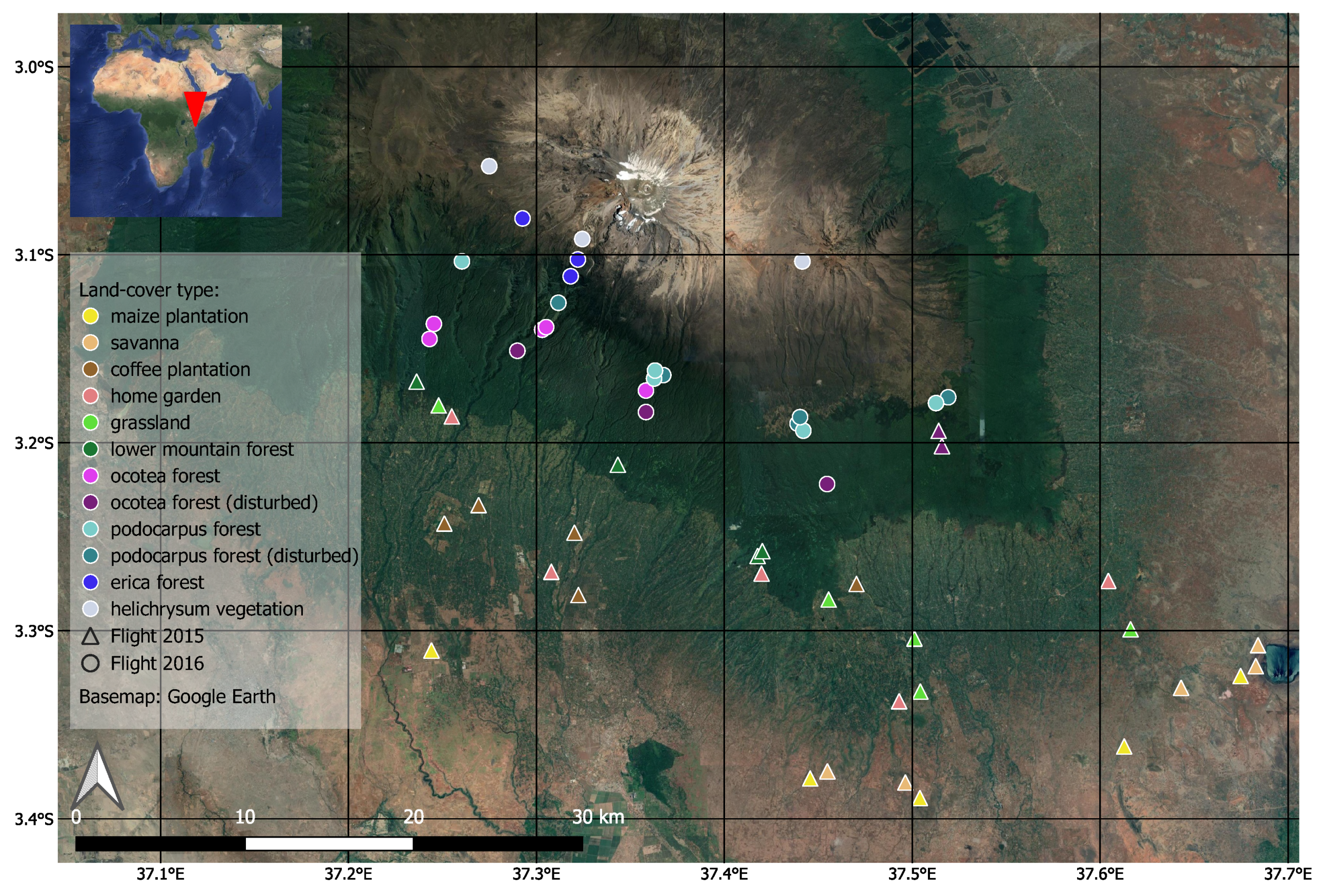
2.1. Study Area and Sampling Design
2.2. Data and Preprocessing
2.2.1. Diversity Data
2.2.2. LiDAR Data
2.3. Predictive Modeling of Diversity
Validation Strategy and Model Tuning
3. Results
4. Discussion
Author Contributions
Funding
Institutional Review Board Statement
Data Availability Statement
Acknowledgments
Conflicts of Interest
Appendix A

| Land Cover | Elevation [m a.s.l] | Number of Plots | Ecosystem |
|---|---|---|---|
| maize plantation | 866–1009 | 5 | non-forest |
| savanna | 871–1153 | 5 | non-forest |
| coffe plantation | 1124–1648 | 5 | non-forest |
| homegarden | 1169–1788 | 5 | non-forest |
| grassland | 1303–1748 | 5 | non-forest |
| lower mountain forest | 1560–2040 | 5 | forest |
| ocotea forest | 2120–2750 | 5 | forest |
| ocotea forest (disturbed) | 2220–2560 | 5 | forest |
| podocarpus forest | 2720–2970 | 5 | forest |
| podocarpus forest (disturbed) | 2770–3060 | 5 | forest |
| erica forest | 3500–3880 | 5 | forest |
| helichrysum vegetation | 3880–4390 | 4 | non-forest |
| Taxon | General Sampling Method | Sampling Specifics | Species Richness Calculation |
|---|---|---|---|
| ants | plastic tubes with diverse set of resource baits on the ground | 2 h at times of peak ant activity | |
| bees | pan traps in different vegetation heights | 48 h with 3 sampling rounds | |
| birds | audiovisual point counts | 15 min before sunrise, completed before 9 am | |
| dung beetles | baited pitfall trap | 72 h sampling time | |
| grass hoppers | sightings and two rounds of sweep net sampling | non-forested ares: repeatedly 1.5 h walking on parallel tracks, forested areas: 1.5 h shaking understory vegetation | sampling effort per site was adjusted to measure asymptotic species richness |
| insectivorous bats | acoustic monitoring (point stop method) | every corner of plot visited for 5 min | averaging species richness values of single surveys |
| large mammals | camera trap, analysis of dung remains | 5 camera trapsper site, 70 trap-days per site | number of all non-domestic mammal species recorded on study site |
| millipedes | pitfall traps and sightings | sightings: 2 h | |
| moths | light traps | 20 min with 4 sampling rounds on obstacle-free branch in 1.5–2 m height | averaging species richness values of single surveys |
| other aculeate wasps | pan traps in different vegetation heights | 48 h with 3 sampling rounds | |
| other beetles | pitfall traps | 7 days sampling time with a total of 5 sampling rounds | |
| parasitoid wasps | pan traps in different vegetation heights | 48 h with 3 sampling rounds | |
| snails | sightings (large taxa) and collection of leaf litter (small taxa) | sightings: four rounds of fixed time surveys of 30 min, collection: 1 litre leaf litter | |
| spiders | pitfall traps | 7 days sampling time | |
| springtails | pitfall traps | 7 days sampling time | |
| syrphid flies | pan traps in different vegetation heights | 48 h with 3 sampling rounds | total (cumulative) number of species richness with varying number of samples among study sites |
| true bugs | sweep net sampling | 100 sweeps along two 50 m transects |
| Decomposer | Generalist | Herbivore | Predator | |
|---|---|---|---|---|
| ants | 0 | 0.24 | 0.02 | 0.02 |
| bees | 0 | 0 | 0.14 | 0 |
| birds | 0 | 0.24 | 0.08 | 0.1 |
| dung beetles | 0.41 | 0 | 0 | 0 |
| grasshoppers | 0 | 0.03 | 0.17 | 0.01 |
| insectivorous bats | 0 | 0 | 0 | 0.02 |
| large mammals | 0 | 0.11 | 0.01 | 0 |
| millipedes | 0.16 | 0 | 0 | 0 |
| moths | 0 | 0 | 0.47 | 0 |
| other aculeate wasps | 0 | 0 | 0 | 0.12 |
| other beetles | 0.24 | 0.37 | 0.07 | 0.17 |
| parasitoid wasps | 0 | 0 | 0 | 0.51 |
| snails | 0.08 | 0.02 | 0.03 | 0.02 |
| syrphid flies | 0.11 | 0 | 0 | 0.02 |
| Decomposer | Generalist | Herbivore | Predator | |
|---|---|---|---|---|
| ants | 0 | 0.47 | 0.24 | 0.29 |
| bees | 0 | 0 | 1 | 0 |
| birds | 0 | 0.18 | 0.31 | 0.51 |
| dung beetles | 1 | 0 | 0 | 0 |
| grasshoppers | 0 | 0.03 | 0.9 | 0.08 |
| insectivorous bats | 0 | 0 | 0 | 1 |
| large mammals | 0 | 0.52 | 0.33 | 0.15 |
| millipedes | 1 | 0 | 0 | 0 |
| moths | 0 | 0 | 1 | 0 |
| other aculeate wasps | 0 | 0 | 0 | 1 |
| other beetles | 0.13 | 0.17 | 0.17 | 0.53 |
| parasitoid wasps | 0 | 0 | 0 | 1 |
| snails | 0.24 | 0.05 | 0.41 | 0.31 |
| syrphid flies | 0.44 | 0 | 0.09 | 0.47 |

References
- Ceballos, G.; Ehrlich, P.R.; Dirzo, R. Biological annihilation via the ongoing sixth mass extinction signaled by vertebrate population losses and declines. Proc. Natl. Acad. Sci. USA 2017, 114, E6089–E6096. [Google Scholar] [CrossRef] [Green Version]
- Pereira, H.M.; Navarro, L.M.; Martins, I.S. Global Biodiversity Change: The Bad, the Good, and the Unknown. Annu. Rev. Environ. Resour. 2012, 37, 25–50. [Google Scholar] [CrossRef] [Green Version]
- Warren, R.; Price, J.; Graham, E.; Forstenhaeusler, N.; VanDerWal, J. The projected effect on insects, vertebrates, and plants of limiting global warming to 1.5 °C rather than 2 °C. Science 2018, 360, 791–795. [Google Scholar] [CrossRef] [PubMed] [Green Version]
- Newbold, T.; Hudson, L.; Hill, S.; Contu, S.; Lysenko, I.; Senior, R.; Börger, L.; Bennett, D.; Choimes, A.; Collen, B.; et al. Global effects of land use on local terrestrial biodiversity. Nature 2015, 520, 45–50. [Google Scholar] [CrossRef] [PubMed] [Green Version]
- Hooper, D.; Chapin, F.; Ewel, J.; Hector, A.; Inchausti, P.; Lavorel, S.; Lawton, J.; Lodge, D.; Loreau, M.; Naeem, S.; et al. Effects of biodiversity on ecosystem functioning: A consensus of current knowledge. Ecol. Monogr. 2005, 75, 3–35. [Google Scholar] [CrossRef]
- Loreau, M.; Naeem, S.; Inchausti, P.; Bengtsson, J.; Grime, J.; Hector, A.; Hooper, D.; Huston, M.; Raffaelli, D.; Schmid, B.; et al. Ecology-Biodiversity and ecosystem functioning: Current knowledge and future challenges. Science 2001, 294, 804–808. [Google Scholar] [CrossRef] [Green Version]
- Soliveres, S.; van der Plas, F.; Manning, P.; Prati, D.; Gossner, M.M.; Renner, S.C.; Alt, F.; Arndt, H.; Baumgartner, V.; Binkenstein, J.; et al. Biodiversity at multiple trophic levels is needed for ecosystem multifunctionality. Nature 2016, 536, 456. [Google Scholar] [CrossRef]
- Nagendra, H.; Lucas, R.; Honrado, J.P.; Jongman, R.H.G.; Tarantino, C.; Adamo, M.; Mairota, P. Remote sensing for conservation monitoring: Assessing protected areas, habitat extent, habitat condition, species diversity, and threats. Ecol. Indic. 2013, 33, 45–59. [Google Scholar] [CrossRef]
- Noss, R. Indicators for Monitoring Biodiversity—A Hierarchical Approach. Conser. Biol. 1990, 4, 355–364. [Google Scholar] [CrossRef]
- Wiens, J.A. Landscape Ecology as a Foundation for Sustainable Conservation. Landsc. Ecol. 2009, 24, 1053–1065. [Google Scholar] [CrossRef]
- Haase, P.; Tonkin, J.D.; Stoll, S.; Burkhard, B.; Frenzel, M.; Geijzendorffer, I.R.; Häuser, C.; Klotz, S.; Kühn, I.; McDowell, W.H.; et al. The next generation of site-based long-term ecological monitoring: Linking essential biodiversity variables and ecosystem integrity. Sci. Total Environ. 2018, 613–614, 1376–1384. [Google Scholar] [CrossRef] [PubMed] [Green Version]
- Jetz, W.; McGeoch, M.; Robert, G.; Ferrier, S.; Beck, J.; Costello, M.; Fernández, M.; Geller, G.; Keil, P.; Merow, C.; et al. Essential biodiversity variables for mapping and monitoring species populations. Nat. Ecol. Evol. 2019, 3, 539–551. [Google Scholar] [CrossRef] [PubMed] [Green Version]
- Pereira, H.M.; Ferrier, S.; Walters, M.; Geller, G.N.; Jongman, R.H.G.; Scholes, R.J.; Bruford, M.W.; Brummitt, N.; Butchart, S.H.M.; Cardoso, A.C.; et al. Essential Biodiversity Variables. Science 2013, 339, 277–278. [Google Scholar] [CrossRef] [Green Version]
- Müller, J.; Brandl, R. Assessing biodiversity by remote sensing in mountainous terrain: The potential of LiDAR to predict forest beetle assemblages. J. Appl. Ecol. 2009, 46, 897–905. [Google Scholar] [CrossRef]
- Kissling, W.D.; Ahumada, J.A.; Bowser, A.; Fernandez, M.; Fernández, N.; García, E.A.; Guralnick, R.P.; Isaac, N.J.B.; Kelling, S.; Los, W.; et al. Building essential biodiversity variables (EBVs) of species distribution and abundance at a global scale. Biol. Rev. 2018, 93, 600–625. [Google Scholar] [CrossRef] [Green Version]
- Proença, V.; Martin, L.J.; Pereira, H.M.; Fernandez, M.; McRae, L.; Belnap, J.; Böhm, M.; Brummitt, N.; García-Moreno, J.; Gregory, R.D.; et al. Global biodiversity monitoring: From data sources to Essential Biodiversity Variables. Biol. Conserv. 2017, 213, 256–263. [Google Scholar] [CrossRef] [Green Version]
- Pettorelli, N.; Wegmann, M.; Skidmore, A.; Mucher, S.; Dawson, T.P.; Fernandez, M.; Lucas, R.; Schaepman, M.E.; Wang, T.; O’Connor, B.; et al. Framing the concept of satellite remote sensing essential biodiversity variables: Challenges and future directions. Remote Sens. Ecol. Conserv. 2016, 2, 122–131. [Google Scholar] [CrossRef]
- Froidevaux, J.S.P.; Zellweger, F.; Bollmann, K.; Jones, G.; Obrist, M.K. From field surveys to LiDAR: Shining a light on how bats respond to forest structure. Remote Sens. Environ. 2016, 175, 242–250. [Google Scholar] [CrossRef] [Green Version]
- Macarthur, R.; Macarthur, J.W. On Bird Species Diversity. Ecology 1961, 42, 594–598. [Google Scholar] [CrossRef]
- Martins, A.C.M.; Willig, M.R.; Presley, S.J.; Marinho-Filho, J. Effects of forest height and vertical complexity on abundance and biodiversity of bats in Amazonia. Forest Ecol. Manag. 2017, 391, 427–435. [Google Scholar] [CrossRef]
- Melin, M.; Hinsley, S.A.; Broughton, R.K.; Bellamy, P.; Hill, R.A. Living on the edge: Utilising lidar data to assess the importance of vegetation structure for avian diversity in fragmented woodlands and their edges. Landsc. Ecol. 2018, 33, 895–910. [Google Scholar] [CrossRef] [Green Version]
- Rocchini, D.; Balkenhol, N.; Carter, G.A.; Foody, G.M.; Gillepsie, T.W.; He, K.S.; Kark, S.; Levin, N.; Lucas, K.; Luoto, M.; et al. Remotely sensed spectral heterogeneity as a proxy of species diversity: Recent advances and open challenges. Ecol. Inform. 2010, 5, 318–329. [Google Scholar] [CrossRef]
- Asner, G.P.; Martin, R.E. Spectranomics: Emerging science and conservation opportunities at the interface of biodiversity and remote sensing. Glob. Ecol. Conserv. 2016, 8, 212–219. [Google Scholar] [CrossRef] [Green Version]
- Mairota, P.; Cafarelli, B.; Labadessa, R.; Lovergine, F.; Tarantino, C.; Lucas, R.; Nagendra, H.; Didham, R. Very high resolution Earth Observation features for monitoring plant and animal community structure across multiple spatial scales in protected areas. Int. J. Appl. Earth Obs. Geoinf. 2015, 37, 100–105. [Google Scholar] [CrossRef]
- Nagendra, H.; Rocchini, D. High resolution satellite imagery for tropical biodiversity studies: The devil is in the detail. Biodivers. Conserv. 2008, 17, 3431–3442. [Google Scholar] [CrossRef]
- Wallis, C.I.B.; Brehm, G.; Donoso, D.A.; Fiedler, K.; Homeier, J.; Paulsch, D.; Suessenbach, D.; Tiede, Y.; Brandl, R.; Farwig, N.; et al. Remote sensing improves prediction of tropical montane species diversity but performance differs among taxa. Ecol. Indic. 2017, 83, 538–549. [Google Scholar] [CrossRef]
- Pettorelli, N.; Laurance, W.; O’Brien, T.; Wegmann, M.; Nagendra, H.; Turner, W. Satellite remote sensing for applied ecologists: Opportunities and challenges. J. Appl. Ecol. 2014, 51, 839–848. [Google Scholar] [CrossRef]
- Lefsky, M.A.; Cohen, W.B.; Parker, G.G.; Harding, D.J. Lidar Remote Sensing for Ecosystem Studies. Bioscience 2002, 52, 19. [Google Scholar] [CrossRef]
- Müller, J.; Vierling, K. Assessing Biodiversity by Airborne Laser Scanning. In Forestry Applications of Airborne Laser Scanning: Concepts and Case Studies; Maltamo, M., Næsset, E., Vauhkonen, J., Eds.; Springer: Dordrecht, The Netherlands, 2014; pp. 357–374. [Google Scholar] [CrossRef]
- Clawges, R.; Vierling, K.T.; Vierling, L.A.; Rowell, E. The use of airborne LiDAR to assess avian species diversity, density, and occurrence in a pine/aspen forest. Remote Sens. Environ. 2008, 112, 2064–2073. [Google Scholar] [CrossRef]
- Flashpohler, D.J.; Giardina, C.P.; Asner, G.P.; Hart, P.; Price, J.; Lyons, C.K. Long-term effects of fragmentation and fragment properties on bird species richness in Hawaiian forests. Biol. Conserv. 2010, 143, 280–288. [Google Scholar] [CrossRef]
- Goetz, S.; Steinberg, D.; Dubayah, R.; Blair, B. Laser remote sensing of canopy habitat heterogeneity as a predictor of bird species richness in an eastern temperate forest, USA. Remote Sens. Environ. 2007, 108, 254–263. [Google Scholar] [CrossRef]
- Jung, K.; Kaiser, S.; Böhm, S.; Nieschulze, J.; Kalko, E.K.V. Moving in three dimensions: Effects of structural complexity on occurrence and activity of insectivorous bats in managed forest stands. J. Appl. Ecol. 2012, 49, 523–531. [Google Scholar] [CrossRef]
- Lesak, A.A.; Radeloff, V.; Hawbaker, T.; Pidgeon, A.M.; Gobakken, T.; Contrucci, K. Follow publication Modeling forest song bird species richness using LiDAR-derived measures of forest structure. Remote Sens. Environ. 2011, 115, 2823–2835. [Google Scholar] [CrossRef]
- Müller, J.; Moning, C.; Bässler, C.; Heurich, M.; Brandl, R. Using airborne laser scanning to model potential abundance and assemblages of forest passerines. Basic Appl. Ecol. 2009, 10, 671–681. [Google Scholar] [CrossRef]
- Müller, J.; Stadler, J.; Brandl, R. Composition versus physiognomy of vegetation as predictors of bird assemblages: The role of LiDAR. Remote Sens. Environ. 2010, 114, 490–495. [Google Scholar] [CrossRef]
- Rechsteiner, C.; Zellweger, F.; Gerber, A.; Breiner, F.T.; Bollmann, K. Remotely sensed forest habitat structures improve regional species conservation. Remote Sens. Ecol. Conserv. 2017, 3, 247–258. [Google Scholar] [CrossRef]
- Vogeler, J.C.; Hudak, A.T.; Vierling, L.A.; Evans, J.; Green, P.; Vierling, K.T. Terrain and vegetation structural influences on local avian species richness in two mixed-conifer forests. Remote Sens. Environ. 2014, 147, 13–22. [Google Scholar] [CrossRef]
- Zellweger, F.; Braunisch, V.; Baltensweiler, A.; Bollmann, K. Remotely sensed forest structural complexity predict multi species occurence at the landscape scale. Forest Ecol. Manag. 2013, 307, 303–312. [Google Scholar] [CrossRef]
- Myers, N.; Mittermeier, R.A.; Mittermeier, C.G.; Da Fonseca, G.A.B.; Kent, J. Biodiversity hotspots for conservation priorities. Nature 2000, 403, 853–858. [Google Scholar] [CrossRef]
- Basset, Y.; Cizek, L.; Cuenoud, P.; Didham, R.; Guilhaumon, F.; Missa, O.; Novotny, V.; Ødegaard, F.; Roslin, T.; Schmidl, J.; et al. Arthropod Diversity in a Tropical Forest. Science 2012, 338, 1481–1484. [Google Scholar] [CrossRef] [Green Version]
- Novotny, V.; Drozd, P.; Miller, S.; Kulfan, M.; Janda, M.; Basset, Y.; Weiblen, G.D. Why are there so many species of herbivorous insects in tropcial rainforests? Nature 2006, 313, 1115–1118. [Google Scholar]
- Peters, M.K.; Hemp, A.; Appelhans, T.; Behler, C.; Classen, A.; Detsch, F.; Ensslin, A.; Ferger, S.W.; Frederiksen, S.B.; Gebert, F.; et al. Predictors of elevational biodiversity gradients change from single taxa to the multi-taxa community level. Nat. Commun. 2016, 7, 13736. [Google Scholar] [CrossRef] [PubMed] [Green Version]
- Vehmas, M.; Eerikäinen, K.; Peuhkurinen, J.; Packalén, P.; Maltamo, M. Identification of boreal forest stands with high herbaceous plant diversity using airborne laser scanning. Forest Ecol. Manag. 2009, 257, 46–53. [Google Scholar] [CrossRef]
- Borthagaray, A.I.; Arim, M.; Marquet, P.A. Connecting landscape structure and patterns in body size distributions. OIKOS 2012, 121, 697–710. [Google Scholar] [CrossRef]
- Morse, D.; Lawton, J.; Dodson, M.; Williamson, M. Fractal Dimension of Vegetation and the Distribution of Arthropod Body Length. Nature 1985, 314, 731–733. [Google Scholar] [CrossRef]
- Siemann, E.; Haarstad, J.; Tilman, D. Dynamics of plant and arthropod diversity during old field succession. Ecography 1999, 22, 406–414. [Google Scholar] [CrossRef]
- Stanska, M.; Stanski, T. Body size distribution of spider species in various forest habitats. Pol. J. Ecol. 2017, 65, 359–370. [Google Scholar] [CrossRef]
- Kaspari, M.; Weiser, M.D. The size–grain hypothesis and interspecific scaling in ants. Funct. Ecol. 1999, 13, 530–538. [Google Scholar] [CrossRef]
- Sarty, M.; Abbott, K.L.; Lester, P.J. Habitat complexity facilitates coexistence in a tropical ant community. Oecologia 2006, 149, 465–473. [Google Scholar] [CrossRef]
- Google Maps. Mt Kilimanjaro, Maxar Technologies (2020), CNES/Airbus (2020). Available online: https://www.google.de/maps/search/kilimanjaro/@-3.094907,37.282672,49189m/data=!3m1!1e3 (accessed on 22 October 2021).
- Peters, M.; Andreas, H.; Appelhans, T.; Becker, J.; Behler, C.; Classen, A.; Detsch, F.; Ensslin, A.; Ferger, S.; Frederiksen, S.B.; et al. Climate–land-use interactions shape tropical mountain biodiversity and ecosystem functions. Nature 2019, 568, 88–92. [Google Scholar] [CrossRef]
- Isenburg, M. LAStools—Efficient LiDAR Processing Software. Available online: http://rapidlasso.com/LAStools (accessed on 22 October 2021).
- Woellauer, S.; Zeuss, D.; Magdon, P.; Nauss, T. RSDB: An easy to deploy open-source web platform for remote sensing raster and point cloud data management, exploration and processing. Ecography 2020, 44, 414–426. [Google Scholar] [CrossRef]
- Jenness, J. Calculating Landscape Surface Area from Digital Elevation Models. Wildl. Soc. Bull. 2004, 32, 829–839. [Google Scholar] [CrossRef]
- Getzin, S.; Fischer, R.; Knapp, N.; Huth, A. Using airborne LiDAR to assess spatial heterogeneity in forest structure on Mount Kilimanjaro. Landsc. Ecol. 2017, 32, 1881–1894. [Google Scholar] [CrossRef]
- Kuhn, M. Caret: Classification and Regression Training, R package version 6.0-80; 2018; Available online: https://cran.r-project.org/web/packages/caret/index.html (accessed on 22 October 2021).
- R Core Team. R: A Language and Environment for Statistical Computing; R Foundation for Statistical Computing: Vienna, Austria, 2018. [Google Scholar]
- Carrascal, L.M.; Galván, I.; Gordo, O. Partial least squares regression as an alternative to current regression methods used in ecology. Oikos 2009, 118, 681–690. [Google Scholar] [CrossRef]
- Laurin, G.V.; Chen, Q.; Lindsell, J.A.; Coomes, D.A.; Frate, F.D.; Guerriero, L.; Pirotti, F.; Valentini, R. Above ground biomass estimation in an African tropical forest with lidar and hyperspectral data. ISPRS J. Photogramm. Remote Sens. 2014, 89, 49–58. [Google Scholar] [CrossRef]
- Luo, S.; Wang, C.; Xi, X.; Pan, F.; Peng, D.; Zou, J.; Nie, S.; Qin, H. Fusion of airborne LiDAR data and hyperspectral imagery for aboveground and belowground forest biomass estimation. Ecol. Indic. 2017, 73, 378–387. [Google Scholar] [CrossRef]
- Næsset, E.; Bollandsås, O.M.; Gobakken, T. Comparing regression methods in estimation of biophysical properties of forest stands from two different inventories using laser scanner data. Remote Sens. Environ. 2005, 94, 541–553. [Google Scholar] [CrossRef]
- Meyer, H. CAST: ’Caret’ Applications for Spatial-Temporal Models, R package version 0.3.1; 2018; Available online: https://cran.r-project.org/web/packages/CAST/index.html (accessed on 22 October 2021).
- Meyer, H.; Reudenbach, C.; Hengl, T.; Katurji, M.; Nauss, T. Improving performance of spatio-temporal machine learning models using forward feature selection and target-oriented validation. Environ. Model. Softw. 2018, 101, 1–9. [Google Scholar] [CrossRef]
- Acebes, P.; Lillo, P.; Jaime-Gonzalez, C. Disentangling LiDAR Contribution in Modelling Species-Habitat Structure Relationships in Terrestrial Ecosystems Worldwide. A Systematic Review and Future Directions. Remote Sens. 2021, 13, 3447. [Google Scholar] [CrossRef]
- Smart, L.S.; Swenson, J.J.; Christensen, N.L.; Sexton, J.O. Three-dimensional characterization of pine forest type and red-cockaded woodpecker habitat by small-footprint, discrete-return lidar. Forest Ecol. Manag. 2012, 281, 100–110. [Google Scholar] [CrossRef]
- Vogeler, J.C.; Hudak, A.T.; Vierling, L.A.; Vierling, K.T. Lidar-derived Canopy Architecture Predicts Brown Creeper Occupancy of Two Western Coniferous Forests. Condor 2013, 115, 614–622. [Google Scholar] [CrossRef]
- Davies, A.B.; Asner, G.P. Advances in animal ecology from 3D-LiDAR ecosystem mapping. Trends Ecol. Evol. 2014, 29, 681–691. [Google Scholar] [CrossRef] [PubMed]
- Vierling, K.T.; Bässler, C.; Brandl, R.; Vierling, L.A.; Weiss, I.; Müler, J. Spinning a laser web: Predicting spider distributions using LiDAR. Ecol. Appl. 2011, 21, 577–588. [Google Scholar] [CrossRef] [PubMed]
- Zellweger, F.; Roth, T.; Bugmann, H.; Bollmann, K. Beta diversity of plants, birds and butterflies is closely associated with climate and habitat structure. Glob. Ecol. Biogeogr. 2017, 26, 898–906. [Google Scholar] [CrossRef]
- McCain, C.M.; Grytnes, J.A. Elevational Gradients in Species Richness. In eLS; American Cancer Society: Atlanta, GA, USA, 2010. [Google Scholar] [CrossRef]
- Müller, J.; Bae, S.; Röder, J.; Chao, A.; Didham, R.K. Airborne LiDAR reveals context dependence in the effects of canopy architecture on arthropod diversity. Forest Ecol. Manag. 2014, 312, 129–137. [Google Scholar] [CrossRef]
- Schooler, S.L.; Zald, H.S.J. Lidar Prediction of Small Mammal Diversity in Wisconsin, USA. Remote Sens. 2019, 11, 2222. [Google Scholar] [CrossRef] [Green Version]

| Name | Explanation |
|---|---|
| canopy | |
| maximum canopy height (CH) | Maximum canopy height |
| mean CH | Mean canopy height |
| median CH | Median canopy height |
| percentile of CH | 10% Percentile of canopy heights |
| …(in 10% steps) | x% Percentile of canopy heights |
| standard deviation CH | Standard Deviation of canopy height |
| skewness CH | Skewness of canopy height Distribution |
| variance CH | Variance of canopy height |
| curtosis CH | Excess Kurtosis of canopy height Distribution |
| coefficient of variation CH | Coefficient of Variation of canopy height |
| area ratio | area ratio of raster pixels (based on CHM) [55] |
| vegetation structure | |
| Return Density (RD) of different layers | Return density of 1 m layer |
| … (1 m steps up to 8 m/29 m) | Return density of x meter layer |
| RD canopy (>5 m) | Return density of canopy vegetation layer |
| RD regeneration (2–5 m) | Return density of regeneration vegetation layer |
| RD understory (<2 m) | Return density of understory vegetation layer |
| RD ground | Return density of ground layer |
| penetration rate (PR) of layers | Penetration rate of 1 m layer |
| … (1 m steps up to 8 m/29 m) | Penetration rate of x meter layer |
| PR canopy (>5 m) | Penetration rate of canopy vegetation layer |
| PR regeneration (2–5 m) | Penetration rate of regeneration vegetation layer |
| PR understory (<2 m) | Penetration rate of understory vegetation layer |
| maximum returns | highest number of return points per LiDAR laser pulse |
| mean returns | mean of return points per LiDAR laser pulse |
| standard deviation returns | standard deviation of return points per LiDAR laser pulse |
| median returns | median of return points per LiDAR laser pulse |
| standard deviation first return | standard deviation of first return points per plot |
| vegetation | |
| above ground biomass | Aboveground Biomass (6.85 ∗ TCH) (top-of-canopy height (TCH) based on CHM) [56] |
| foliage height diversity | Foliage height diversity (Shannon Index grouped by layers of understory, regeneration and canopy) [19] |
| leaf area index | Leaf-area index, with k = 0.3, h.bin = 1, GR.threshold = 5 (based on CHM) [56] |
| vegetation coverage (VC) of different layers | vegetation coverage in 1 m height (based on CHM) |
| …(for 2, 5, and 10 m) | vegetation coverage in x meter height (based on CHM) |
| gap fraction | fraction of clear area above 10 m compared to whole area (to be detected as gap: minimum of 9 cells, based on CHM) |
| Model Name | Independent Variables (Predictors) | Target Variables (Response) |
|---|---|---|
| elevation | elevation, elevation 2 | species richness |
| structure | structural LiDAR variables | species richness |
| residuals | structural LiDAR variables | residuals from elevation model |
| combination | sum of elevation model and structural model | species richness |
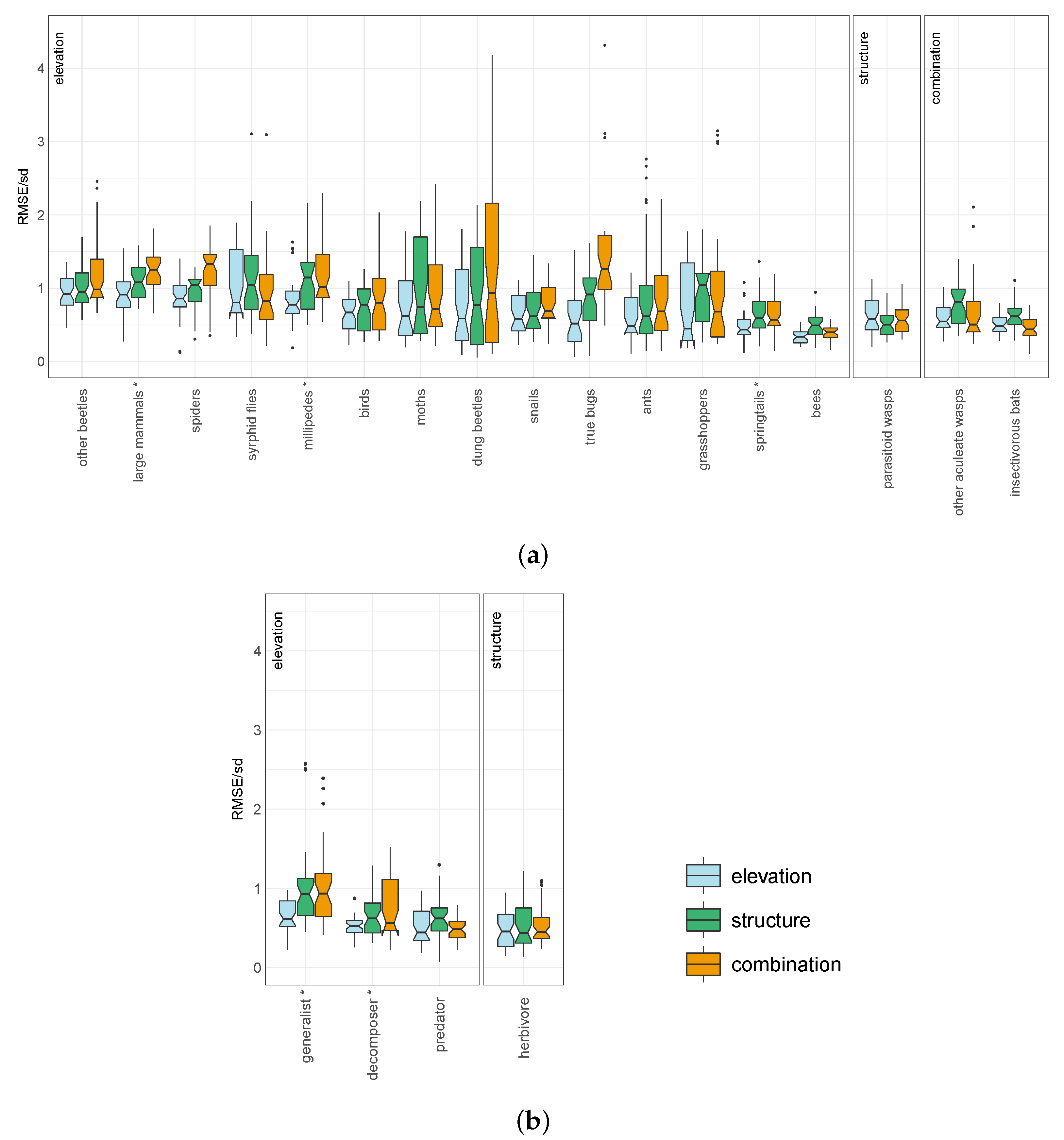
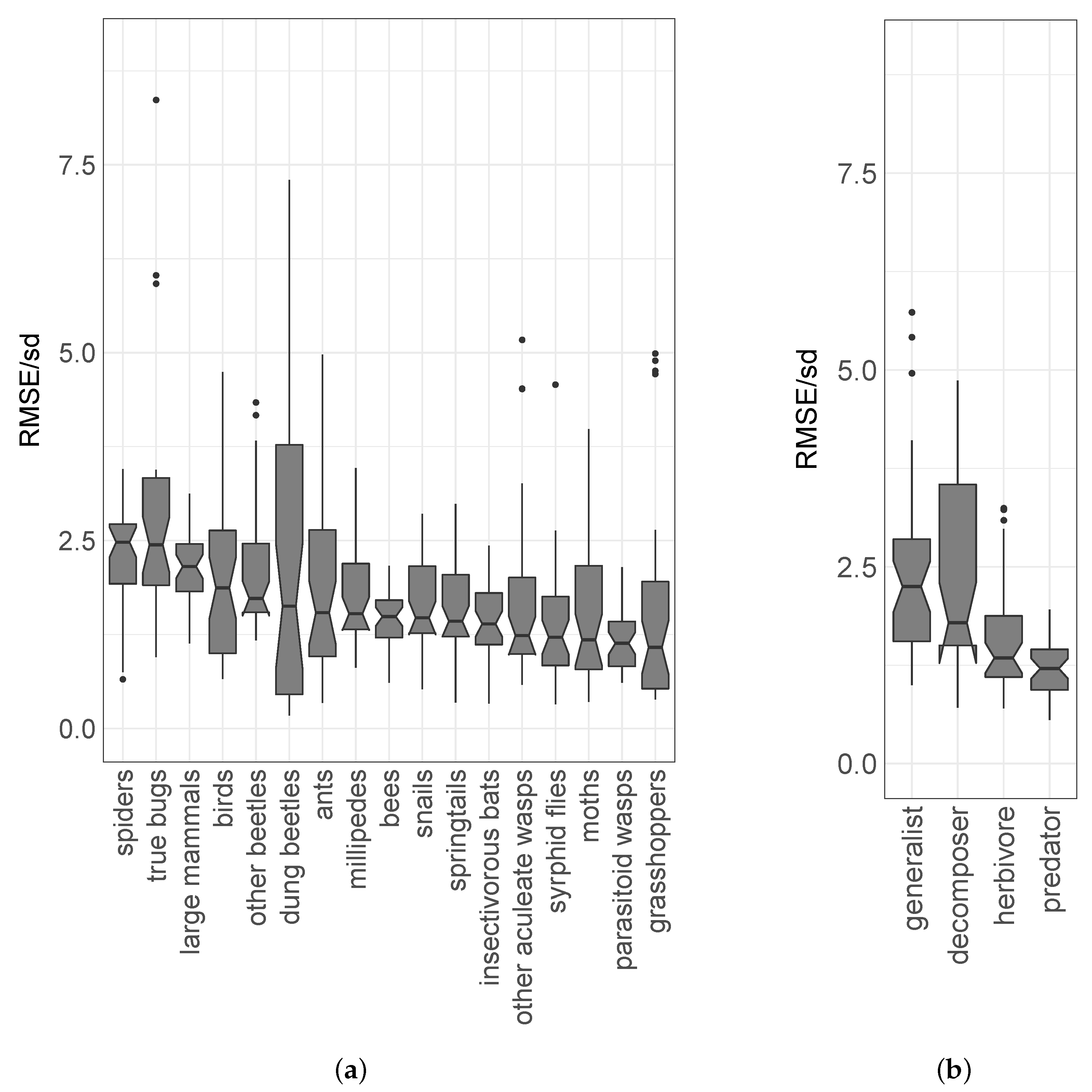
| Taxon/Feeding Guild | Species Richness per Plot | Elevation Model | Structure Model | Combined Model | Residual Model |
|---|---|---|---|---|---|
| Mean ± Standard Deviation | Median RMSE/sd ± Standard Deviation | ||||
| ants | 2.7 ± 3.4 | 0.48 ± 0.29 | 0.62 ± 0.72 | 0.69 ± 0.57 | 1.5 ± 1.3 |
| bees | 6.7 ± 5.9 | 0.34 ± 0.1 | 0.49 ± 0.17 | 0.4 ± 0.11 | 1.5 ± 0.4 |
| birds | 16 ± 8.6 | 0.67 ± 0.25 | 0.77 ± 0.31 | 0.8 ± 0.45 | 1.9 ± 1 |
| dung beetles | 5.2 ± 7.7 | 0.59 ± 0.5 | 0.77 ± 0.73 | 0.93 ± 1.3 | 1.6 ± 2.2 |
| grasshoppers (locusts, crickets) | 10 ± 14 | 0.45 ± 0.54 | 1 ± 0.41 | 0.68 ± 0.82 | 1.1 ± 1.3 |
| insectivorous bats | 5.5 ± 3.3 | 0.48 ± 0.13 | 0.62 ± 0.18 | 0.44 ± 0.14 | 1.4 ± 0.46 |
| large mammals | 2.3 ± 1.8 | 0.91 ± 0.28 | 1.1 ± 0.24 | 1.3 ± 0.26 | 2.2 ± 0.45 |
| millipedes | 1.2 ± 1.7 | 0.77 ± 0.34 | 1.1 ± 0.48 | 1 ± 0.43 | 1.5 ± 0.65 |
| moths | 9.6 ± 11 | 0.62 ± 0.48 | 0.74 ± 0.69 | 0.72 ± 0.61 | 1.2 ± 1 |
| other aculeate wasps | 3.2 ± 4 | 0.55 ± 0.21 | 0.82 ± 0.26 | 0.5 ± 0.45 | 1.2 ± 1.1 |
| other beetles | 8.6 ± 4.9 | 0.92 ± 0.24 | 0.95 ± 0.27 | 0.98 ± 0.46 | 1.7 ± 0.81 |
| parasitoid wasps | 16 ± 14 | 0.58 ± 0.26 | 0.5 ± 0.18 | 0.56 ± 0.19 | 1.1 ± 0.38 |
| snails (slugs) | 6.8 ± 5.6 | 0.58 ± 0.26 | 0.62 ± 0.31 | 0.69 ± 0.28 | 1.5 ± 0.61 |
| spiders | 5 ± 2.2 | 0.86 ± 0.26 | 1 ± 0.23 | 1.3 ± 0.39 | 2.5 ± 0.72 |
| springtails | 4.6 ± 2.4 | 0.43 ± 0.2 | 0.59 ± 0.27 | 0.57 ± 0.25 | 1.4 ± 0.63 |
| syrphid flies | 3.5 ± 3.3 | 0.8 ± 0.47 | 1 ± 0.55 | 0.82 ± 0.5 | 1.2 ± 0.74 |
| true bugs | 2.1 ± 2.3 | 0.57 ± 0.39 | 0.91 ± 0.37 | 1.3 ± 1.1 | 2.4 ± 2.2 |
| decomposer | 12 ± 7.8 | 0.53 ± 0.13 | 0.62 ± 0.25 | 0.56 ± 0.38 | 1.8 ± 1.2 |
| generalist | 6.8 ± 3.8 | 0.61 ± 0.21 | 0.93 ± 0.57 | 0.94 ± 0.48 | 2.2 ± 1.2 |
| herbivore | 40 ± 30 | 0.46 ± 0.23 | 0.44 ± 0.3 | 0.45 ± 0.26 | 1.3 ± 0.77 |
| predator | 41 ± 22 | 0.44 ± 0.22 | 0.62 ± 0.23 | 0.48 ± 0.15 | 1.2 ± 0.37 |
| Body Size | Mode of Movement | |||
|---|---|---|---|---|
| r | p | p | ||
| RMSE/sd elevation | −0.14 | 0.58 | 0.28 | |
| RMSE/sd structure | −0.13 | 0.62 | 0.28 | |
| RMSE/sd combination | −0.10 | 0.70 | 0.011 | (flying <non-flying) |
| RMSE/sd residuals | −0.22 | 0.39 | 0.006 | (flying <non-flying) |
Publisher’s Note: MDPI stays neutral with regard to jurisdictional claims in published maps and institutional affiliations. |
© 2022 by the authors. Licensee MDPI, Basel, Switzerland. This article is an open access article distributed under the terms and conditions of the Creative Commons Attribution (CC BY) license (https://creativecommons.org/licenses/by/4.0/).
Share and Cite
Ziegler, A.; Meyer, H.; Otte, I.; Peters, M.K.; Appelhans, T.; Behler, C.; Böhning-Gaese, K.; Classen, A.; Detsch, F.; Deckert, J.; et al. Potential of Airborne LiDAR Derived Vegetation Structure for the Prediction of Animal Species Richness at Mount Kilimanjaro. Remote Sens. 2022, 14, 786. https://doi.org/10.3390/rs14030786
Ziegler A, Meyer H, Otte I, Peters MK, Appelhans T, Behler C, Böhning-Gaese K, Classen A, Detsch F, Deckert J, et al. Potential of Airborne LiDAR Derived Vegetation Structure for the Prediction of Animal Species Richness at Mount Kilimanjaro. Remote Sensing. 2022; 14(3):786. https://doi.org/10.3390/rs14030786
Chicago/Turabian StyleZiegler, Alice, Hanna Meyer, Insa Otte, Marcell K. Peters, Tim Appelhans, Christina Behler, Katrin Böhning-Gaese, Alice Classen, Florian Detsch, Jürgen Deckert, and et al. 2022. "Potential of Airborne LiDAR Derived Vegetation Structure for the Prediction of Animal Species Richness at Mount Kilimanjaro" Remote Sensing 14, no. 3: 786. https://doi.org/10.3390/rs14030786
APA StyleZiegler, A., Meyer, H., Otte, I., Peters, M. K., Appelhans, T., Behler, C., Böhning-Gaese, K., Classen, A., Detsch, F., Deckert, J., Eardley, C. D., Ferger, S. W., Fischer, M., Gebert, F., Haas, M., Helbig-Bonitz, M., Hemp, A., Hemp, C., Kakengi, V., ... Nauss, T. (2022). Potential of Airborne LiDAR Derived Vegetation Structure for the Prediction of Animal Species Richness at Mount Kilimanjaro. Remote Sensing, 14(3), 786. https://doi.org/10.3390/rs14030786