Article

Spatiotemporal and Multiscale Analysis of the Coupling Coordination Degree between Economic Development Equality and Eco-Environmental Quality in China from 2001 to 2020

1
School of Geography Science and Geomatics Engineering, Suzhou University of Science and Technology, Suzhou 215009, China
2
College of Resources and Environment, Xingtai University, Xingtai 054001, China
3
Xingtai Key Laboratory of Geo-information and Remote Sensing Technology Application, Xingtai 054001, China
4
Aerospace Information Research Institute, Chinese Academy of Sciences, Beijing 100094, China
5
College of Mathematics and Informatics, Fujian Normal University, Fuzhou 350108, China
6
Piesat Information Technology Company Limited, Beijing 100195, China
7
School of Civil Architectural Engineering, Shandong University of Technology, Zibo 255000, China
8
College of Urban and Environmental Sciences, Peking University, Beijing 100871, China
9
Department of Geography and Environmental Studies, Wollo University, Dessie, Ethiopia
10
School of Resource and Environment, Hunan University of Technology and Business, Changsha 410205, China
*
Author to whom correspondence should be addressed.
These authors contributed equally to this work and should be considered co-first authors.
Remote Sens. 2022, 14(3), 737; https://doi.org/10.3390/rs14030737
Submission received: 3 December 2021 / Revised: 19 January 2022 / Accepted: 28 January 2022 / Published: 4 February 2022
(This article belongs to the Special Issue Remote Sensing Imagery for Mapping Economic Activities)

Abstract

:
Evaluating and exploring regional eco-environmental quality (EEQ), economic development equality (EDE) and the coupling coordination degree (CCD) at multiple scales is important for realizing regional sustainable development goals. The CCD can reflect both the development level and the interaction relationship of two or more systems. However, relevant previous studies have ignored non-statistical data, lacked multiscale analyses, misused the coupling coordination degree model or have not sufficiently considered economic development equality. In response to these problems, this study integrated multisource remote sensing datasets to calculate and analyse the remote sensing ecological index (RSEI) and then used nighttime light data and population density data to calculate the proposed nighttime difference index (NTDI). Next, a modified coupling coordination degree (MCCD) index was proposed to analyse the MCCD between EEQ and EDE. Then, spatiotemporal and multiscale analyses at the county, city, province, urban agglomeration and country levels were performed. Global and local spatial autocorrelation and trend analyses were performed to evaluate the spatial aggregation degree and change trends from 2001 to 2020. The main conclusions are as follows: (1) The EEQ of China displayed a fluctuating upwards trend (0.0048 a−1), with average RSEI values of 0.5950, 0.6277, 0.6164, 0.6311 and 0.6173; the EDE of China showed an upwards trend (0.0298 a−1), with average NTDI values of 0.1271, 0.1635, 0.1642, 0.2181 and 0.2490; and China’s MCCD indicated an upwards trend (0.0220 a−1), with values of 0.4614, 0.5027, 0.4978, 0.5401 and 0.5525. (2) The highest global Moran’s I of NTDI and MCCD was achieved at the city scale, while the highest RSEI was achieved at the county scale. From 2001 to 2020, the spatial agglomeration effect of the RSEI decreased, while that of the NTDI and MCCD increased. (3) A power function relationship occurred between NTDI and MCCD at different scales. Furthermore, the NTDI had a higher contribution to improving the MCCD than the RSEI and the R2 of the fitted curve at different scales ranged from 0.8183 to 0.9915.

1. Introduction

Since the implementation of the reform and opening-up policy in 1978, China has experienced tremendous changes, especially in terms of urbanization development [1]. According to the China Statistical Yearbook (2021) issued by the National Bureau of Statistics, the urbanization rate of China increased from 17.92% in 1978 to 63.89% in 2020 [2]. Based on the United Nations’ report, the world’s population living in urban areas is expected to reach 66% in 2050 [3]. However, with the acceleration of urbanization, the population density has also increased, which has caused excessive resource consumption [4]. Accordingly, several problems have been observed, such as the deterioration of the eco-environment [5], degradation of land quality [6], increased number of natural disaster cases [7] and a widening economic development gap among different regions [8]. These problems have hindered the realization of sustainable development goals [9]. In response to these problems, China’s government promulgated the regional coordinated development strategy in 2017 [1]. However, due to the complexity of urbanization and eco-environment subsystems, the coupling coordination relationship between them remains to be explored [10]. Hence, it is urgent to investigate their relationship and spatiotemporal change trends.
The eco-environment is defined as “the total quantity and quality of water resources, land resources, biological resources and climate resources that affect human survival and development” and it represents a social–economic–natural compound system [11]. Evaluations of eco-environmental quality (EEQ) include the construction of an appropriate index system based on certain standards and scientific evaluations of the regional EEQ [12]. At present, existing studies can be mainly divided into two types. The first mainly utilizes statistical data to evaluate regional EEQ; for example, Fu systematically evaluated the EEQ of China [13]. The second mainly applies remote sensing and other geospatial data to assess regional EEQ; for example, He et al. developed a comprehensive evaluation index to assess urban EEQ changes [14]. The urbanization level evaluation method can also be divided into two types. The first mainly adopts several statistical datasets to evaluate a city’s urbanization level; for example, Chen et al. selected 16 indicators from 4 aspects (population, land, society and economy) to assess China’s urbanization level [15] and Zang et al. also selected 16 indicators to evaluate the urbanization level of Jilin Province from 4 aspects, population, economy, spatiality and society [16]. The second mainly utilizes remote sensing data to assess the regional urbanization level; for example, Sun et al. adopted nighttime images to evaluate urbanization processes between China and India from 1992 to 2013 [17]. Numerous studies have been performed on the relationship between urbanization and EEQ. For example, Sarkodie and Strezov conducted an empirical study of the environmental Kuznets curve hypothesis (EKC) [18] and Li et al. explored the coupling coordination degree (CCD) between urbanization and ecosystems [19]. Several theories have also been proposed, such as the environmental Kuznets curve [20], urban metabolism theory [21], footprint family theory [22], tele-coupling theory [23], planetary boundaries theory [24], coupling coordination degree model (CCDM) [25], stochastic impacts by regression on population, affluence and technology model [26] and multi-agent model [27]. Among these theories, the EKC and CCDM have been widely used. The EKC indicates that an inverted “U” shape occurs between per capita income and EEQ. Although researchers have validated this hypothesis [28,29,30], other researchers have indicated that this hypothesis was not supported in their studies because the EKC fails to consider the interaction between urbanization and EEQ [31]. Compared with the EKC theory, the CCDM considers the interaction between two or more subsystems [32]. Coupling, originating from physics, is a phenomenon in which two or more subsystems in a whole physical system affect each other via miscellaneous interactions [33,34]. To date, the CCDM has been widely applied in exploring the coupling relationships between different subsystems. For example, Li assessed the coordinated development level of the economy, society and environment subsystem in a city [35]; Xie et al. analysed the coordinated development of the “resources-environment-ecology-economy-society” complex system in China [36]; and Shen et al. assessed the CCD between carbon emissions and EEQ [37].
Previous studies on EEQ evaluation, urbanization level assessment and exploration of their relationship have achieved fruitful results. However, certain limitations were observed. (a) Existing studies have mainly utilized statistical data to evaluate regional EEQ or urbanization level. Statistical data have the advantage of high authority; however, they may also include incomplete statistical indicators and inconsistent statistical calibres and may not be able to perceive spatial distributions. More importantly, statistical data can only be acquired at the administrative level and data at the pixel level cannot be acquired. Compared with statistical data, remote sensing data have the advantages of long time series and wide spatial distributions. For example, Ji et al. utilized MODIS data and constructed a remote sensing ecological index (RSEI) to assess the EEQ of the Jing–Jin–Ji urban agglomeration [11,12] and Xu et al. combined multisource remote sensing data to investigate the coupling mechanism between EEQ and urbanization [10]. (b) Existing studies have mainly analysed their results at one scale and thus lacked multiscale analyses. Scale effects are widely observed in geography; thus, it is important to investigate CCD at various scales. (c) Existing studies on urbanization level assessments have mainly focused on the economy and few have focused on economic development equality (EDE). (d) Several researchers have misused the CCDM [38]. In addition, the CCDM has only been used to calculate the geometric mean of the coupling degree and comprehensive development level, which has failed to distinguish cases with different coupling degrees and comprehensive development levels but the same CCD.
Therefore, in response to these shortcomings, this paper combined remote sensing data and the RSEI to evaluate China’s EEQ. Next, nighttime light data and population density data were utilized to calculate the proposed nighttime difference index (NTDI). Then, a modified coupling coordination degree index was proposed to analyse the modified coupling coordination degree (MCCD) between EDE and EEQ. Finally, spatiotemporal and multiscale analyses at the county, city, province, urban agglomeration and country levels were performed. Global and local spatial autocorrelation and trend analyses were also performed to evaluate the spatial aggregation degree and change trend from 2001 to 2020. This paper is organized as follows: the section Material and Methods describes the study area and methods, which include the methods for calculating the RSEI, NTDI, MCCD, global and local spatial autocorrelation and change trend; the section Results presents the spatiotemporal distribution, spatial autocorrelation and change trend of the RSEI, NTDI and MCCD at four scales; the section Discussion validates the RSEI, investigates the relationship among the RSEI, NTDI and MCCD and presents the implications and limitations of this study; the section Conclusion presents the main findings of this paper.

2. Materials and Methods

2.1. Study Area

China is located in east Asia (73°29′~135°20′E, 3°31′~53°33′N), covers approximately 9.6 million km2 (Figure 1) and includes 23 provinces, 5 autonomous regions, 4 municipalities and 2 special administrative regions. China has diverse terrain, different climate types and complex natural conditions [39]. In addition, China is one of the countries with the richest biodiversity in the world [40]. Regarding the population and economy, China is the most populous country and the second largest economy in the world, with approximately 1.4 billion people and 15.9 trillion dollars GDP in 2020. In this study, Hong Kong, Macao and Taiwan were excluded and only mainland China and Hainan Province were analysed.

2.2. Data Sources

In this study, multiple remote sensing datasets and administrative division data were collected, which are shown in Table 1.
According to Table 1, the MOD09A1 product provides an estimate of the surface spectral reflectance of Terra MODIS bands 1–7 at a 500 m resolution and corrected for atmospheric conditions. The MOD11A2 product provides an average 8-day land-surface temperature (LST) at a 1000 m resolution [11,12]. In addition, to exclude the phenology effect [41,42], the data collection period was from 1 June to 31 August because Zhang et al. found that the annual RSEI change trend was similar to the average RSEI value in summer [43]. NPP-VIIRS-like nighttime light data were acquired from Chen’s study [44] and they were produced through a new cross-sensor calibration method, having better spatial resolution (500 m). WorldPop data were acquired from the WorldPop website. WorldPop provides the yearly population density spatial distribution data at a resolution of 1000 m. Administrative division data provided the boundary of different levels in shapefile format. In this study, the EEQ, EDE and MCCD of 31 provincial administrative regions, 366 cities, 2842 counties and 19 urban agglomerations were analysed.

2.3. Data Methods

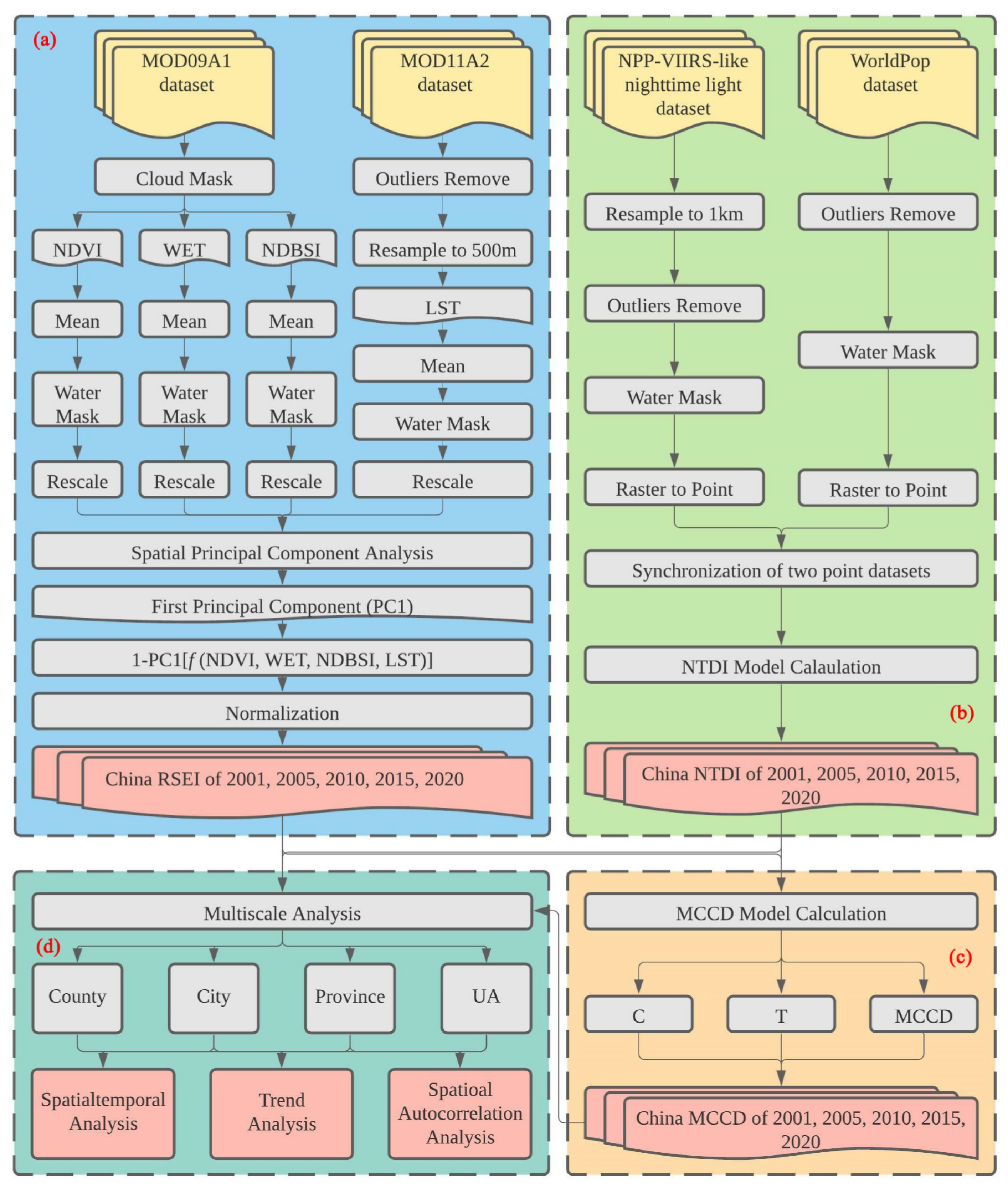
Figure 2 presents the framework of this study, which includes the following four parts: (a) RSEI calculation; (b) NTDI calculation; (c) MCCD calculation; (d) spatiotemporal, spatial autocorrelation, change trend and multiscale analyses. Among them, RSEI and NTDI were performed at the country scale and then each region’s RSEI value was acquired by calculating the average RSEI values of all grids in this region. Based on each region’s RSEI and NTDI values, the MCCD was calculated. Section 2.3.1, Section 2.3.2, Section 2.3.3, Section 2.3.4 and Section 2.3.5 introduce the calculation formulas in detail.

2.3.1. Calculation of the RSEI

The RSEI was promoted by Xu in 2013 [45]. It consists of four subindicators, normalized difference vegetation index (NDVI), wetness (WET), normalized difference build-up and soil index (NDBSI) and LST. Equations (1)–(6) were used to acquire mainland China’s RSEI in 2001, 2005, 2010, 2015 and 2020 [11]. All equations were calculated using the Google Earth Engine platform and ArcGIS 10.6 software.
NDVI = ρ nir ρ red / ρ nir + ρ red
WET = 0.1084 × ρ red + 0.0912 × ρ nir + 0.5065 × ρ blue + 0.4040 × ρ green 0.2410 × ρ mir 1 0.4658 × ρ mir 2 0.5306 × ρ mir 3
NDSBI = 1 2 2 × ρ mir 2 ρ mir 2 + ρ nir ρ nir ρ nir + ρ red ρ green ρ green + ρ mir 2 2 × ρ mir 2 ρ mir 2 + ρ nir + ρ nir ρ nir + ρ red + ρ green ρ green + ρ mir 2 + 1 2 ρ mir 2 + ρ red ρ nir ρ blue ρ mir 2 + ρ red + ρ nir + ρ blue
RSEI origin = 1 PC 1 f NDVI , WET , NDBSI , LST
X rescale = X i X min / X max X min
RSEI = RSEI origin _ i RSE I min / RSEI max RSEI min
where ρ stands for the surface reflectance bands; blue, green, red, nir, mir1, mir2 and mir3 are the MODIS bands at 459–479 nm, 545–565 nm, 620–670 nm, 841–876 nm, 1230–1250 nm, 1628–1652 nm and 2105–2155 nm, respectively; PC1 represents the first component of the spatial principal component analysis (SPCA); LST denotes the land-surface temperature acquired from MOD11A2; Xrescale indicates the normalized result of each index; and RSEI means the normalized result of the RSEIorgin.

2.3.2. Calculation of the NTDI

Traditional methods mainly utilize nighttime light data to evaluate a city’s urbanization level; however, nighttime light data cannot reflect the equality of different cities because population density is not considered in these data. The Gini coefficient has been widely applied to estimate income equality [46]. Equation (7) presents the Gini coefficient calculation equation.
Gini = 1 2 y ¯ u 1 n n 1 i n j n y i y j
where y i and y j represent the per capita GDP for regions i and j, and y ¯ u indicates the mean value of per capita GDP for n regions. The Gini coefficient ranges from 0 to 1 and a larger value corresponds to a more equal distribution of GDP. Theoretically, Gini coefficients of 1 and 0 represent absolute inequality and absolute equality, respectively. To allow the highest value to represent the highest equality, NPP-VIIRS-like nighttime light data and WorldPop data were combined and this paper proposes the NTDI. Equation (8) presents the calculation formula.
N T D I = 1 1 2 N T ¯ 1 n n 1 i n j n N T i N T j
where N T j and N T i represent the per capita nighttime light value for regions i and j, and N T ¯ indicates the mean value of the per capita nighttime light value for n regions. The per capita nighttime light value was obtained at the pixel level by dividing the light value by the population density value.

2.3.3. Calculation of the MCCD

The CCDM has been widely applied to analyse the coupling coordination degree. Equations (9)–(11) present the calculation formulas.
C = 2 × U 1 × U 2 U 1 + U 2 2 1 2
T = α × U 1 + β × U 2
D = C × T
where C represents the coupling degree; U1 and U2 represent two subsystems; T indicates the comprehensive development level of U1 and U2; α and β represent the weights of U1 and U2, respectively; and α + β = 1. In this study, α and β were set as 0.5 and D denotes the coupling coordination degree.
Although the CCDM considers the interaction of two or more subsystems, it only calculates the geometric mean of C and T. However, it cannot differentiate cases with different C and T but the same D, such as when C equals to 0.90, 0.30 and 0.10 and T equals to 0.10, 0.30 and 0.90, but D equals to 0.30 in all cases. To solve this problem, this paper proposes a modified coupling coordination degree (MCCD) index to calculate the MCCD from the perspective of distance. Equation (12) presents the calculation formula.
M C C D = 2 × C × T C 2 + T 2
where MCCD represent the modified coupling coordination degree and ranges from 0 to 1. In addition, a higher MCCD corresponds to a higher level of coupling coordination degree between U1 and U2. In this study, U1 and U2 indicate the RSEI and NTDI values, respectively.

2.3.4. Calculation of Spatial Autocorrelation

Spatial autocorrelation describes the correlation between a variable at a specific position and its neighbouring position. A positive spatial correlation occurs when one observed spatial value changes in the same direction as the surrounding values and a negative spatial correlation occurs when these two values are inversely related. A random distribution occurs when the observed values show randomness in spatial distribution, thus indicating that the spatial correlation is not apparent. Spatial autocorrelation can be measured at the global and local levels [12]. Equations (13)–(14) present the calculation methods.
I g = N i j w i j x i μ x j μ i j w i j i x i μ 2
I l = x i μ i x i μ 2 j w i j x j μ
where xi and xj represent the variable values at i and j; μ is the average value; wij is the spatial weight function; and N is the number of sample pairs. In this paper, the inverse distance method was adopted to conceptualize the spatial relationship, the Euclidean distance was selected as the distance method, the number of permutations was set to 499 and the exponent was set to 1.

2.3.5. Trend Analysis Method

In this study, a trend analysis was performed to quantitatively evaluate the change trends of the RSEI, NTDI and MCCD. The principle of the trend analysis is to analyse the change trend and intensity of a variable by performing a univariate linear regression analysis. Among them, the slope of the regression equation represents the variable’s change trend [47,48]. Compared with the Mann–Kendall trend test and Sen’s slope, the trend analysis method has the advantage of simplicity and low sample size requirements [48]. In this paper, only five periods were performed. For the Mann–Kendall trend test and Sen’s slope methods, the sample size normally needs to be higher than 10 [49,50]. Equation (15) presents the calculation formula.
θ s l o p e = n × i = 1 n i × N i i = 1 n i i = 1 n N i n × i = 1 n i 2 i = 1 n i 2
where θslope indicates the change trend; n is the number of study periods and equals 5 in this study; Ni is the ith value of the RSEI, NTDI and MCCD. θslope > 0 represents an increasing trend; and θslope ≤ 0 represents a decreasing trend.

3. Results

3.1. Spatiotemporal and Change Trends of the RSEI at Different Scales

The average RSEI values of China in the five periods were 0.5950, 0.6277, 0.6164, 0.6311 and 0.6173, which showed a fluctuating upwards trend with a change rate of 0.0048. This finding indicates that the EEQ of China has improved over the past 20 years. Figure 3 displays the spatial distribution of the RSEI and its change trend from 2001 to 2020 at different scales.
At the different scales, the spatial distribution of the RSEI was similar. Specifically, at the county scale, the RSEI was higher in northeastern, central and southern China while the RSEI was lower mainly in northwestern and north China. Over the past 20 years, counties along the Yangtze River mainly showed a negative change rate, while counties in Shanxi and Inner Mongolia mainly displayed a positive change rate. In addition, counties in western Shandong, Chengdu and Yunnan also showed a negative change rate. In 2001, 6.68% and 2.28% of all counties belonged to the first and last grades, respectively, while, in 2020, 7.42% and 1.19% of all counties were in the first and last grades, respectively. In 2020, counties in the first three grades increased while counties in the last two grades decreased compared with 2001. At the city scale, higher RSEI values were mainly distributed in northeastern, central and southern China and lower RSEI values were mostly observed in northwestern China. Cities in Shanxi, Ningxia and Inner Mongolia had higher change trends, indicating that their EEQ had improved. Chengdu, Meishan and cities along the Yangtze River showed a downwards tendency from 2001 to 2020. Most cities of Xinjiang, Qinghai and Guangdong also showed a positive trend but with a lower value. The highest and lowest change trend values were 0.0389 and −0.0217, respectively, indicating that the RSEI value of all cities did not drastically change. In 2001, 5.46% and 2.73% of cities belonged to the first and last grades, respectively. Compared with 2001, the percentage of cities belonging to these two grades in 2020 changed by 1.09% and −1.37%. At the province scale, from 2001 to 2020, the RSEI values of Heilongjiang and Jilin belonged to the first grade in five periods, while Xinjiang was always in the last grade. The RSEI of Shanxi improved by two grades, thus showing an upwards trend. In addition, Inner Mongolia, Ningxia, Shaanxi and Gansu also had a higher change trend, indicating that these provinces’ EEQ had improved. However, the provinces of Jiangsu, Shanghai, Zhejiang, Hubei, Jiangxi and Hunan displayed a downwards trend. From 2001 to 2020, the highest and lowest change trend values were 0.0245 and −0.0127, respectively. At the urban agglomeration scale, in 2001, the three urban agglomerations including northern Tianshan, northern Ningxia and central Inner Mongolia belonged to the last grade, while, in 2020, the RSEI grade of the three urban agglomerations improved. The Harbin–Changchun urban agglomeration was always in the first grade. The Yangtze River Delta and central Changjiang urban agglomerations showed a negative change trend. In addition, Shandong Peninsula, Chengdu Chongqing, central Guizhou, central Yunnan and the west coast urban agglomerations also showed negative values. Inner Mongolia and central Shanxi and Guanzhong urban agglomerations had a higher change trend value and the highest and lowest change trend values from 2001 to 2020 were 0.0227 and −0.0109, respectively.

3.2. Spatiotemporal and Change Trends of the NTDI at Different Scales

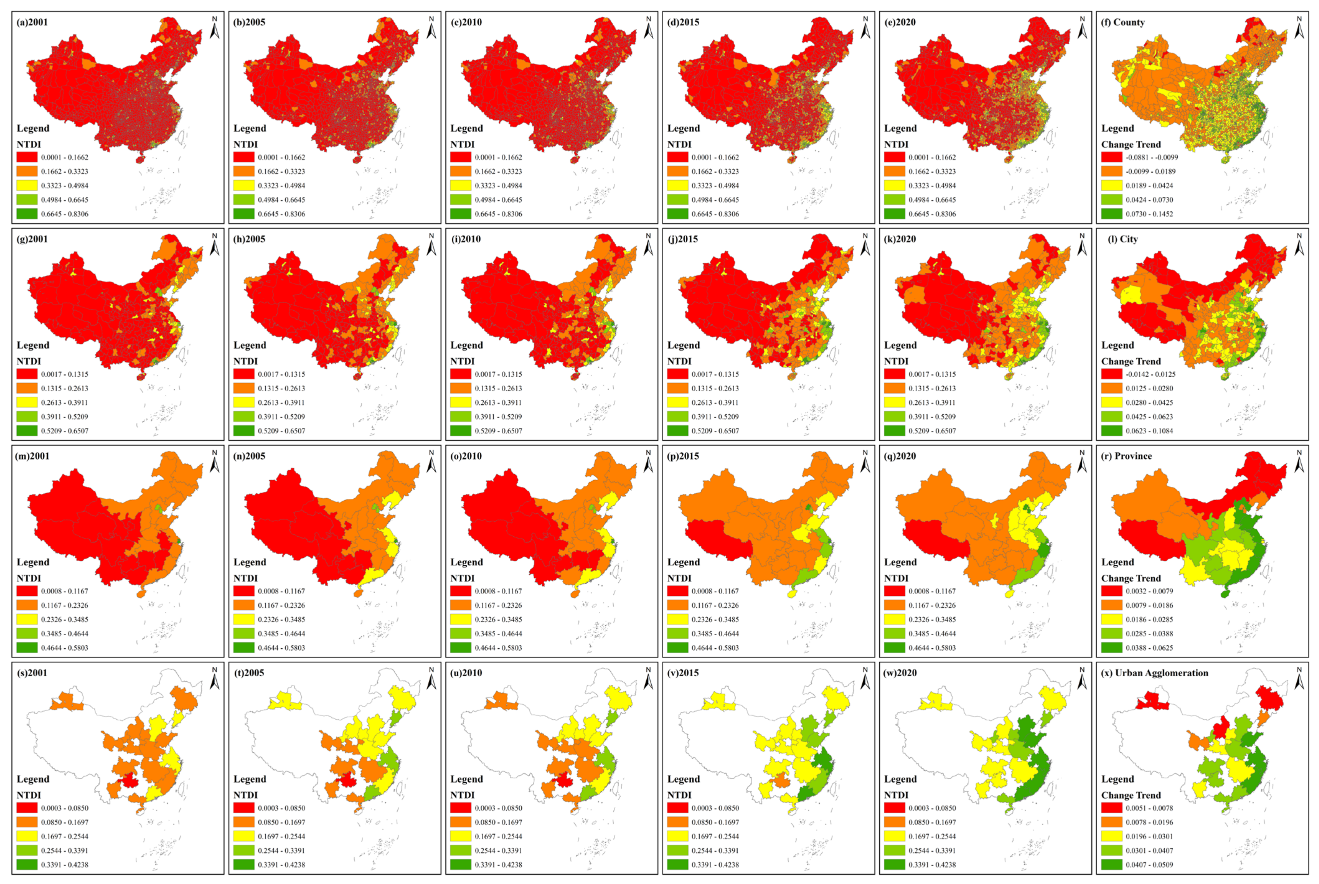
The average NTDI values of China in the five periods were 0.1271, 0.1635, 0.1642, 0.2181 and 0.2490, with a change trend value of 0.0298. Compared with 2001, the average NTDI value increased by 95.91% in 2020, indicating that the EDE improved gradually. Figure 4 shows the spatial distribution and change trend of the NTDI from 2001 to 2020 at different scales.
At the county scale, from 2001 to 2020, counties with higher NTDI values were mainly distributed in Beijing, Tianjin, southern Jiangsu, northern Zhejiang, Shanghai and the Pearl River Delta. Other counties with higher NTDI values were sporadically located in the main districts of cities with better economies, for example, provincial capital. In 2001, 75.22% and 4.43% of counties belonged to the last and the first two grades, respectively, while, in 2020, 40.46% and 10.69% of counties belonged to these grades, respectively. In addition, 34.76% of the counties’ grades had improved. The eastern coastal counties showed a positive change trend with higher values, while northeastern, northwestern and western Sichuan and Xizang had lower change values. Specifically, 90.57% of counties had a positive change value, indicating that most counties’ economic development equality had narrowed. At the city scale, over the past 20 years, cities with higher NTDI values were mainly distributed in the eastern coastal region, while cities with lower NTDI values were mostly located in northwestern and southwestern China. In 2001, 2.45% of all cities belonged to the first two grades, while 66.39% of all cities belonged to the last grade. In 2020, 14.21% of all cities belonged to the first two grades, while 19.12% of all cities belonged to the last grade. Cities with higher change trend values were mainly distributed in southern Jiangsu, central Shandong, eastern Henan, northern Zhejiang, eastern Fujian, eastern Sichuan and western Guangdong. Cities with lower change trend values were mainly located in Xizang, northwestern Xinjiang, northern Inner Mongolia and northeastern China. Generally, 96.45% of cities showed a positive change trend. At the province scale, Beijing, Tianjin and Shanghai always belonged to the first grade, while Xizang always belonged to the last grade. In 2001, all remaining provinces except Beijing, Tianjin and Shanghai belonged to the last two grades. In 2020, only half of the provinces belonged to the last two grades and seven provinces’ NTDI belonged to the top two grades. For the NTDI change trend, the NTDI of all provinces displayed a positive value. Specifically, Hebei, Shandong, Jiangsu, Zhejiang, Fujian, Guangdong and Hainan had higher change values, followed by Ningxia, Shaanxi, Sichuan, Guizhou, Guangxi, Henan and Anhui, while Xizang, Inner Mongolia, Heilongjiang and Jilin had lower change values. Beijing and Tianjin had relatively low change values, although both cities belonged to the top two grades in all periods. At the urban agglomeration scale, from 2001 to 2020, the NTDI values of urban agglomerations along the coastal region, including Beijing–Tianjin–Hebei, Shandong Peninsula, Yangtze River Delta, west Coast and Pearl River Delta, were substantially improved. In 2001, all urban agglomerations belonged to the last three grades, while, in 2020, more than half of the urban agglomerations belonged to the top two grades. All urban agglomerations displayed an upwards change trend. Specifically, the Shandong Peninsula, Yangtze River Delta and west Coast urban agglomerations had a higher trend value, followed by the Beijing–Tianjin–Hebei, central plain, northern Ningxia, Pearl River Delta, southern Guangxi, Chengdu–Chongqing and central Guizhou urban agglomerations, while the central Inner Mongolia, Harbin–Changchun and northern Tianshan urban agglomerations had a lower trend value.

3.3. Spatiotemporal and Change Trends of the MCCD at Different Scales

The average MCCD values of China in the five periods were 0.4614, 0.5027, 0.4978, 0.5401 and 0.5525, with a change trend value of 0.0220. Compared with 2001, the average MCCD value increased by 19.74% in 2020, indicating that the coupling coordination relationship between EDE and EEQ has improved over the past 20 years. Figure 5 shows the spatial distribution and change trend of the MCCD from 2001 to 2020 at different scales.
At the county scale, over the past 20 years, eastern coastal counties had a higher MCCD value. In addition, counties in Liaodong Peninsula, central Shanxi, northern Henan, main urban areas of Chengdu, Chongqing and other provincial capital cities also showed a higher MCCD. In 2001, 28.85% and 25.12% of all counties belonged to the top two and last two grades, respectively. In 2020, 69.59% and 5.38% of all counties were in the top two and last two grades, respectively. Compared with 2001, counties in the top two grades increased by 40.74% in 2020. A total of 91.91% of all counties showed a positive change trend value, indicating that the MCCD between EDE and EEQ had improved. However, counties with a negative trend value were mainly distributed in northeastern Heilongjiang and sporadically distributed in other areas. Furthermore, counties with a higher trend value were mainly distributed in central Guizhou, western Hunan, western Sichuan, southern Qinghai, southern Gansu, southern Shaanxi, eastern Fujian, northeastern Guangdong and southern Xizang. At the city scale, eastern coastal cities displayed a higher MCCD value, for example, Beijing, Tianjin, Shanghai, southern Jiangsu, northern Zhejiang, eastern Fujian and eastern Guangdong. Cities with a lower MCCD value were mainly distributed in Xinjiang, northwestern Gansu, northwestern Inner Mongolia and western Xizang. In 2001, 27.59% and 24.31% of all cities belonged to the top two and last two grades, respectively. In 2020, 73.22% and 5.19% of all cities belonged to the top two and last two grades, respectively. Compared with 2001, cities in the top two grades increased by 45.63%, while cities in the last two grades decreased by 19.12% in 2020. A total of 97.54% of cities displayed a positive change trend. Cities with a negative change trend were Hegang, Daxinganling, Yichun, Baishan, Tonghua, Changchun, Shihezi, Hulunbuir and Urumqi. At the province scale, Beijing and Shanghai always belonged to the first grade. Xizang and Xinjiang were always in the last two grades. In 2001, eleven and eight provinces belonged to the last two and top two grades, respectively. In 2020, two and twenty-three provinces belonged to the last two and top two grades, respectively. The eastern coastal provinces had a higher MCCD grade, followed by the northeastern and central provinces. Inner Mongolia, Yunnan and western China’s provinces had a lower MCCD grade. All provinces displayed a positive change trend value. Specifically, Xinjiang, Inner Mongolia, Heilongjiang, Jilin, Liaoning, Beijing, Tianjin and Shanghai had lower change trend values, while Shaanxi, Shanxi, Ningxia, Sichuan, Guizhou, Hainan, Guangdong, Zhejiang and Fujian had higher change trend values, followed by Gansu, Hebei, Shandong, Henan and Guangxi. At the urban agglomeration scale, in 2001, the four urban agglomerations northern Tianshan, northern Ningxia, central Guizhou and central Inner Mongolia were in the last grade and three urban agglomerations belonged to the second grade. In 2020, seven urban agglomerations, almost all along the coastal area, were in the first grade and only two urban agglomerations belonged to the last two grades—northern Tianshan and central Inner Mongolia. All urban agglomerations displayed a positive change trend. Specifically, the northern Tianshan, Harbin–Changchun and Liaodong Peninsula urban agglomerations had a lower trend value, while the Guanzhong, northern Ningxia, central Guizhou and west Coast urban agglomerations had a higher trend value, followed by the Pearl River Delta, Shandong Peninsula, central Plain, central Shanxi, southern Guangxi and Chengdu–Chongqing urban agglomerations.

3.4. Spatial Autocorrelation Analysis of the RSEI, NTDI and MCCD at Different Scales

Table 2 shows the global Moran’s I value at different scales.
The global Moran’s I value varied with the scale and index. Specifically, for the RSEI, the average global Moran’s I values at the four scales were 0.2663, 0.2865, 0.0864 and 0.0660. This indicates that the RSEI showed a higher spatial agglomeration effect at the city scale but a lower spatial agglomeration effect at the province and urban agglomeration scales. In summary, the global Moran’s I value of the RSEI displayed an inverted “U” shape as the scale increased. For the NTDI, the average global Moran’s I value represented an upwards shape, indicating that the spatial agglomeration effect decreased as the scale increased. For the MCCD, a similar change trend of the average Moran’s I value was found. The global Moran’s I value of the RSEI showed an upward-shaped change trend, while the NTDI and MCCD displayed an inverted “U” shape. The NTDI and MCCD showed a higher spatial agglomeration effect at the city level. In addition, the RSEI change trend at the county scale displayed a strong spatial agglomeration effect, with a global Moran’s I value of 0.6189.
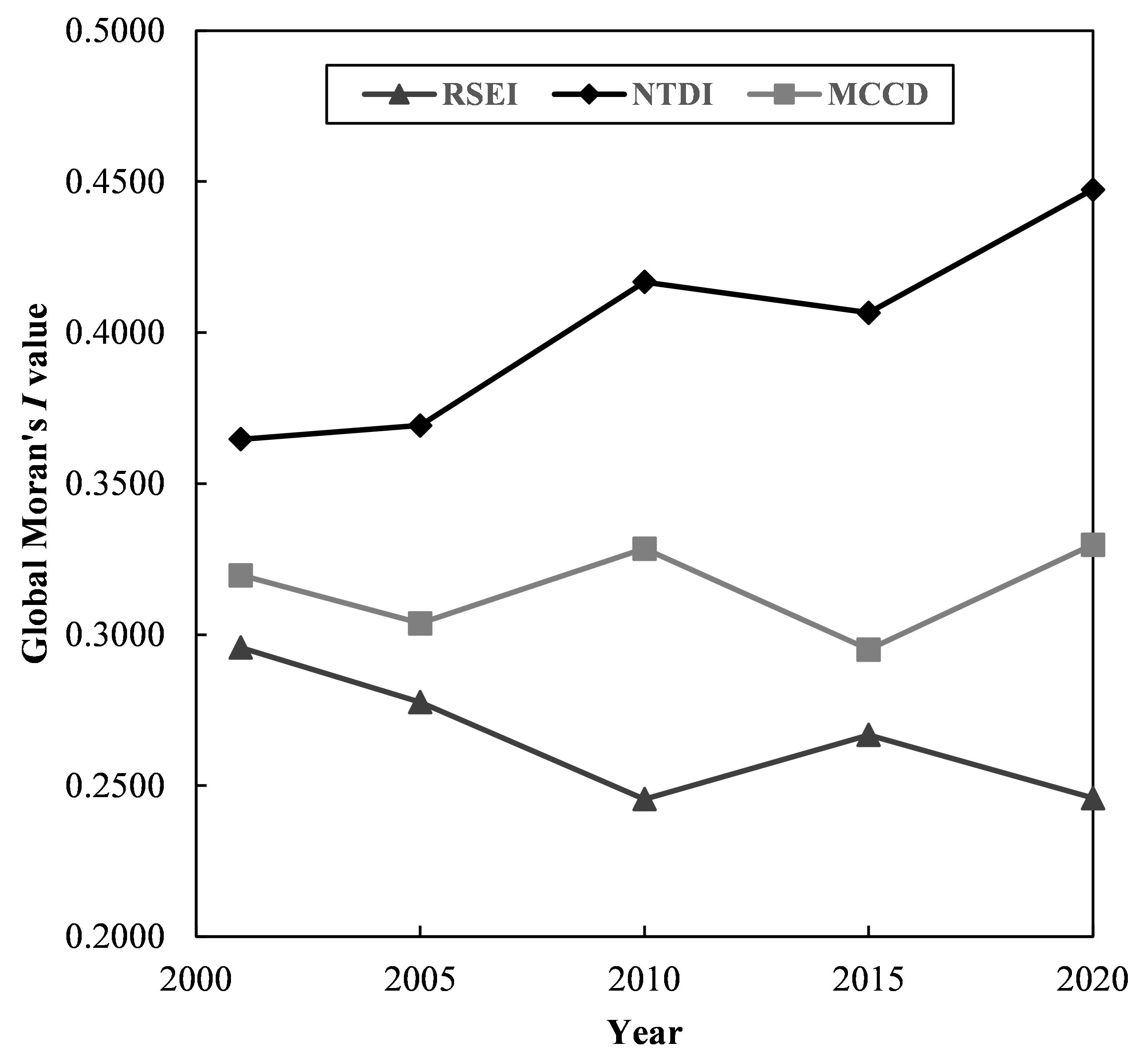
Figure 6 shows the global Moran’s I value change trend from 2001 to 2020 at the county scale. The global Moran’s I value of the RSEI displayed a downwards trend, while the NTDI showed an upwards trend. For the MCCD, it displayed a fluctuating upwards trend. Generally, the spatial agglomeration effect of the RSEI decreased from 2001 to 2020, while that of the NTDI and MCCD increased. In particular, the spatial agglomeration effect of the NTDI greatly increased, with the global Moran’s I value increasing by 22.68%.
Figure 7 shows the local Moran’s I spatial distribution of the RSEI, NTDI and MCCD from 2001 to 2020 at the county scale. For the RSEI, from 2001 to 2020, the high–high cluster type was mainly distributed in northeastern and central China, while the low–low cluster type was mainly distributed in northwestern China, southwestern Xizang and Inner Mongolia. Compared with 2001, the low–low cluster type expanded in Jiangsu, Henan and Hebei, while the high–high cluster type shrank in Hubei, Yunnan, Guangxi and Guizhou in 2020. These counties are mainly located in eastern and central China. For the NTDI, over the past 20 years, high–high cluster counties were mainly observed in eastern China, including the Yangtze River Delta, west Coast, Pearl River Delta, Shandong Peninsula, Beijing–Tianjin–Hebei and central plain. However, the low–low cluster type was mainly located in central China, Xizang, western Xinjiang, Qinghai, Shaanxi, Gansu and northeastern Inner Mongolia and Heilongjiang. Among them, northeastern Inner Mongolia and Heilongjiang were newly expanded areas, indicating that these regions’ NTDI values were lower. Furthermore, the low–low cluster type decreased in the Chengdu–Chongqing urban agglomeration. As one of five large urban agglomerations of China, Chengdu–Chongqing presented a gradually improved EDE over the past 20 years. For the MCCD, from 2001 to 2020, the high–high cluster type was mainly in eastern China and central Henan, while the low–low cluster type was mainly distributed in western China, Inner Mongolia and central China. Generally, compared with 2001, the high–high cluster type in northeastern China decreased, while the low–low cluster type in the Chengdu–Chongqing urban agglomeration, Hubei, Hunan, Shannxi, Guangxi and Jiangxi decreased in 2020. Furthermore, Hainan was a newly expanded region with a high–high cluster type. For the change trend of the RSEI, the high–high cluster type was mainly distributed in Gansu, Ningxia, Shannxi, Shanxi, Inner Mongolia and Guangdong, while the low–low cluster type was mainly distributed in these regions along the Yangtze River, Chengdu and Yunnan. Regarding the change trend of the NTDI, the high–high cluster type was mainly distributed in the eastern coastal areas and Chengdu, while the low–low cluster type was mainly distributed in Xizang, Qinghai, Xinjiang and northeastern China. Regarding the change trend of the MCCD, the high–high cluster type was mainly observed in Sichuan, Chongqing, Guizhou, Guangxi, southern Shaanxi and eastern Xizang, while the low–low cluster type was mainly distributed in northern Xinjiang, northern Inner Mongolia and northeastern China.

4. Discussion

4.1. Spatial Principal Component Analysis of the RSEI and Its Validation

Based on the aforementioned analysis, an SPCA of the RSEI was performed; then, ecological index (EI) data of Guangdong Province in 2010, 2015 and 2019 were collected. Next, the relationship between the EI and RSEI data was investigated.
Table 3 shows the SPCA results for the RSEI from 2001 to 2020. According to Table 3, all four indicators had a stable positive or negative symbol. The eigenvalues of the four indicators in different years all showed relatively high values. In all years, the NDVI and WET had a positive effect on the regional EEQ, while the NDBSI and LST had a negative effect. These results are consistent with numerous previous studies. For example, Yuan et al. found that the loadings of the NDVI and WET were all positive, while the loadings of the NDBSI and LST were negative [51]; Gao et al. also showed that the load values of the NDVI and WET were positive, while the load values of NDBSI and LST were negative [52]; and Xiong et al. found that the loadings of the NDVI and WET were positive, while the loadings of NDBSI and LST were negative in the Erhai Lake Basin [53]. Generally, different studies reached the same results regarding the loading effect of the four indicators; however, regarding the contribution percentage of PC1, the results have varied. In general, the range of PC1’s contribution rate was higher than 60% [51,52,53,54,55]. In this study, the contributions percentage of the five periods were 66.26% (2001), 63.57% (2005), 63.89% (2010), 65.79% (2015) and 65.69% (2020). Similar to previous studies, PC1 aggregated the most information of the four indicators with an average contribution percentage of 65.04%. To further validate the results of the RSEI, a comparison between the RSEI and EI was conducted. The EI was promulgated by the Ministry of Environmental Protection, China in 2015 [56]. However, calculating the EI is complicated. Therefore, due to EI data accessibility, the EI values of Guangdong Province in 2010, 2015 and 2019 were utilized for validation. Among them, the EI value of 2019 was used to perform a correlation analysis with the RSEI in 2020. Figure 8 shows the relationship between the EI and RSEI of Guangdong Province in 2010, 2015 and 2020.
According to Figure 8, in 2010, 2015 and 2020, the R2 values in the three periods were 0.4335, 0.7987 and 0.9089, with an average R2 of 0.7137. This finding indicates that the EI was strongly correlated with the RSEI. Existing studies have also validated the effectiveness of the RSEI at a large scale. For example, Ji et al. selected the Jing–Jin–Ji urban agglomeration as the study area to compare the RSEI and EI values at the urban agglomeration scale and found that the RSEI and EI displayed the same change trend [11]. Xu et al. chose Fujian Province as the study area to explore the relationship between the RSEI and EI and found that the RSEI was comparable to the EI at either the index value or grade [56]. Shan et al. compared the RSEI and EI of well-facilitated farmland and found that the index values were similar [57]. However, Xu et al. found that the RSEI was significantly underestimated based on the bias value and concluded that the traditional RSEI was not applicable at a large scale [10]. In general, similar to numerous previous studies, the RSEI and EI were comparable. In addition, four indicators of the RSEI were directly derived from remote sensing images, which was more convenient and efficient [42]. However, as for the inapplicability of RSEI at large scale, He et al. chose the RSEI to evaluate and validate China’s EEQ [39] and they found that areas with a decreasing trend were mainly in the Yangtze River Delta, central northern China Plain and central Xizang, which is consistent with this study. Hence, although differences can be observed among previous studies, the result of the SPCA and the comparison between the RSEI and EI indicate the feasibility of evaluating China’s EEQ based on the RSEI.

4.2. Relationship among the RSEI, NTDI and MCCD

To explore the relationship among the RSEI, NTDI and MCCD, data for all years were used to draw a three-dimensional diagram at different scales using Unscrambler X 10.4 software (Figure 9). Specifically, the number of samples at different scales was as follows: 14,210 (county), 1830 (city), 155 (province) and 95 (urban agglomeration).
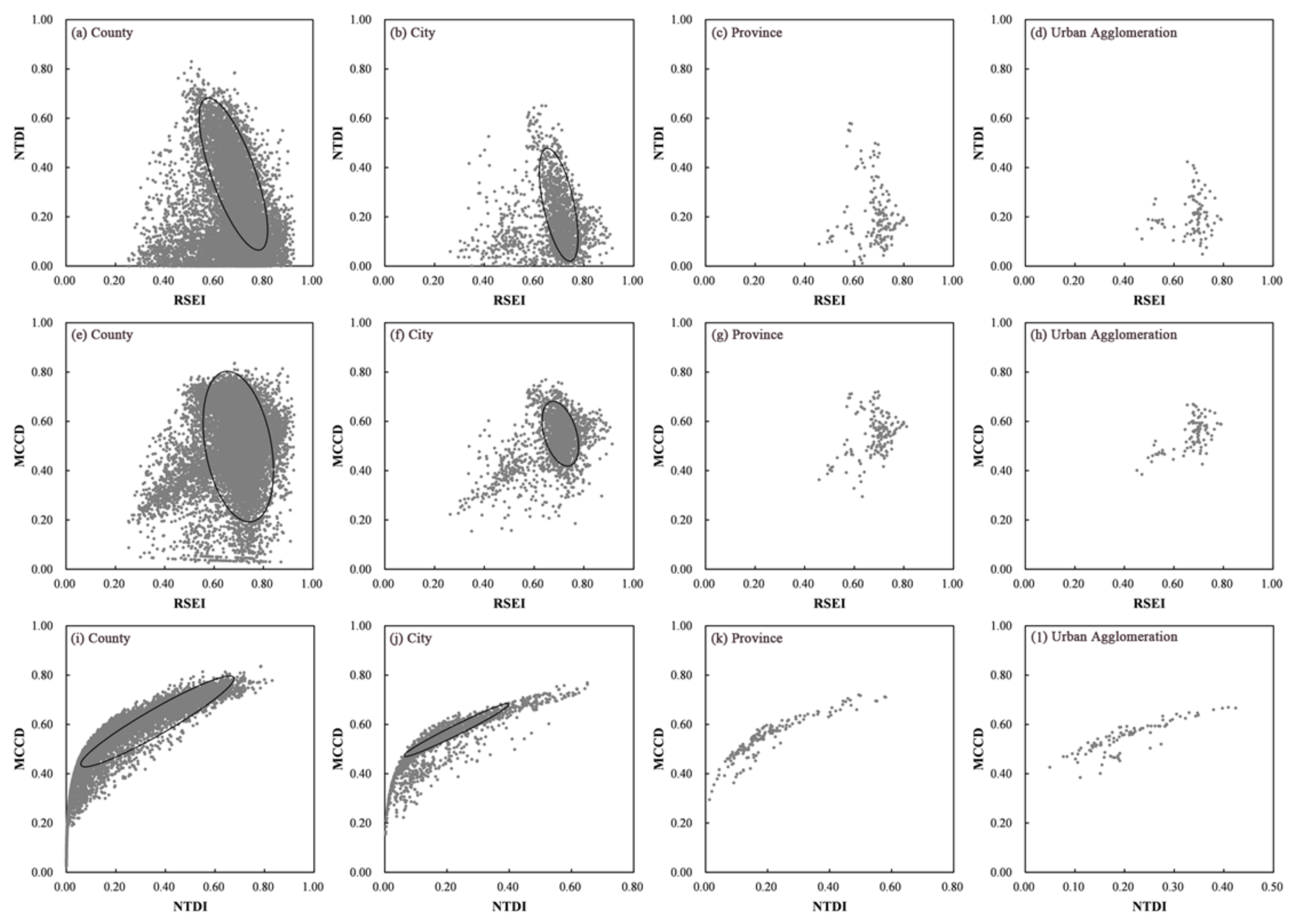
Based on Figure 9, the relationship among the RSEI, NTDI and MCCD seemed to show a saddle-shape distribution. To explore any two sets of relationships, scatter plots of the RSEI, NTDI and MCCD at four scales were drawn (Figure 10).
Based on Figure 10, the relationship of the RSEI and NTDI at different scales seemed to be negative, the relationship of the RSEI and MCCD did not show a correlation distribution, while the relationship of the NTDI and MCCD displayed a power function distribution. To explore the relationship of the RSEI, NTDI and MCCD, a multiple linear regression was performed at different scales. Fitting formulas were acquired and are displayed in Table 4.
Based on Table 4, the coefficients of RSEI and NTDI were all positive, indicating that improving the RSEI or NTDI would promote a region’s MCCD. However, compared with the RSEI, the NTDI had a higher contribution. For example, at the county scale, when a region’s NTDI increased by one unit, the MCCD would increase by 0.7831; however, when a region’s RSEI increased by one unit, the MCCD would only increase by 0.4521. In addition, the adjusted R2 showed an upwards tendency as the scale increased. To test the model accuracy, a scatter plot between the original and predicted MCCD was drawn (Figure 11).
Based on Figure 11, the original and predicted MCCD at four scales showed a good relationship with R2 values of 0.8183 (county), 0.9275 (city), 0.9732 (province) and 0.9915 (urban agglomeration). However, at the county and city scales, the predicted MCCD would be overestimated when the original MCCD was too low or too high. Generally, the fitting formula could well predict the MCCD when the original MCCD value was in the mid-range. Previous studies have explored the relationship of urbanization rate, EEQ and CCD. Specifically, Xu et al. explored the relationship between urbanization rate and CCD and found that they showed an inverted “U” shape; however, critical values for numerous cities were not observed until the urbanization rate exceeded 100% [10]. However, the highest value of urbanization rate was 100%. Hence, although there was a difference between the NTDI and Xu’s urbanization rate evaluation methods, the power function could well demonstrate the relationship for both approaches [10]. Fang et al. did not identify a stable functional relationship between the urbanization rate and EEQ at the urban agglomeration scale [58]. These results indicate that the relationship between urbanization and EEQ depended on the specific study area, which is consistent with this paper’s results. In this study, although a weak negative correlation coefficient was observed between the NTDI and RSEI, these indices could not be fitted by any function. In addition, the power function relationship between the NTDI and MCCD was further confirmed. Moreover, this paper found that the RSEI and NTDI had a positive effect on the regional MCCD at different scales; however, the NTDI had a higher contribution.

4.3. Implications, Limitations and Further Research

This study aims to explore the relationship of the RSEI, NTDI and MCCD. Based on the RSEI results, northeastern and southern China mainly had higher EEQ, while Xinjiang and Qinghai had lower EEQ. This finding is consistent with the vegetation coverage distribution of China. According to statistical bulletins on the national economic and social development of each province in 2021 [2], there were fifteen provinces with a forest coverage rate greater than 40%. In addition, Beijing, Shaanxi, Heilongjiang and Jilin were located in the northern China, while the remaining eleven provinces were located in the south. Based on the Qinling Mountains–Huaihe River line, mainland China was divided into south and north. The average RSEI value of southern China in all periods was 0.6974, which was higher than that of northern China (0.6654). The difference was not large, because the summer season was chosen to calculate the RSEI. This difference would be larger in winter because the vegetation type in the north is mainly deciduous forest. Generally, southern China had better EEQ than northern China. For the change trend, regions along the Yangtze River and part of Chengdu had a negative value. Generally, the economic development level of regions along the Yangtze River was relatively good compared with that in other regions of in China. However, these regions consumed higher energy, which exerted considerable pressure on the regional eco-environment. In addition, the Chengdu Plain, as an important economic centre in southeastern China, consumed considerable energy. Ningxia, Shanxi, Shaanxi, Gansu and Inner Mongolia had positive trend values, which is mainly due to the implementation of the “Three-North Shelter Forest Program” [11]. Since this program was launched in 1978, forestland increased by 30.14 million hectares. For Ningxia, Shanxi, Shaanxi, Gansu and Inner Mongolia, the total forestland areas were 1.67 million hectares by 2020 [2]. In addition, combined with He’s study, the RSEI value of Shanxi increased considerably, while that of Shanghai decreased considerably [39], which further validates this paper’s results.
For the NTDI, over the past 20 years, coastal provinces, including Jiangsu, Shanghai, Zhejiang, Fujian, Guangdong, Beijing and Tianjin, showed considerably increased values. Based on the NTDI-change-trend spatial distribution map, almost all coastal provinces had the highest change trend value, followed by central China and northeastern and northwestern China. In addition, the average NTDI values of the whole country in the five periods were 0.1271, 0.1635, 0.1642, 0.2181 and 0.2490, indicating that the EDE of China narrowed. Based on the statistical yearbook of each province, the coefficient of variation of China’s urbanization rate in the five periods was 0.3794 (2001), 0.3269 (2005), 0.2940 (2010), 0.2202 (2015) and 0.1707 (2020), indicating that the EDE of China had narrowed, which further validates this paper’s results [2]. In view of the highest NTDI change trend value of Zhejiang Province, each city’s urbanization rate in the five periods was determined. The coefficients of variation in the five periods were 0.2179 (2001), 0.1784 (2005), 0.1505 (2010), 0.1109 (2015) and 0.1074 (2020). Over the past 20 years, the coefficient of variation decreased by 50.71%, which is consistent with this paper’s findings. Regarding the MCCD, the coupling coordination degree between EEQ and EDE, based on Figure 5, the MCCD of China at the province scale in 2020 displayed a stepped distribution. The MCCD grade almost decreased from the east to west. Coastal provinces had a higher MCCD, followed by the central, northeastern and southern provinces. Northern and western provinces had a lower MCCD. Combined with the RSEI, although regions along the Yangtze River showed a negative change trend, these regions had a higher MCCD because of their higher NTDI. The aforementioned analysis showed that the NTDI had a higher contribution to improving the MCCD than the RSEI at different scales. Generally, this finding provides important guidance for government policy making.
Despite these implications, this study still has some limitations that need to be further explored. (a) The scientific evaluations of regional EEQ include numerous aspects. The RSEI only considers four main aspects, greenness, wetness, dryness and heat. However, other aspects, such as air quality or land-use intensity also play an important role in EEQ assessments. The RSEI has its own shortcomings and it cannot fully cover and capture the eco-environmental situation. For example, shrub invasion might be accompanied by an increase in greenness; however, the RSEI could not distinguish the greening caused by eco-environmental degradation from the greening caused by eco-environmental improvement [39]. In addition, water needs to be masked before performing the SPCA to exclude its influence on the final evaluation result [57]. However, water resources, as important ecological resources, play a key role in climate regulation, vegetation irrigation, the terrestrial water cycle and ecosystem balance [59]. Therefore, methods considering the eco-environmental function of water need to be explored in the future. (b) This paper only explores the relationship among the RSEI, NTDI and MCCD. However, accurately predicting the future coupling coordination degree is more important. Therefore, combining dynamic models or other methods to scientifically predict the MCCD remains to be investigated.

5. Conclusions

This study utilized multisource remote sensing datasets to evaluate the RSEI, NTDI and MCCD at multiple scales from 2001 to 2020. The main conclusions are as follows: (1) China’s EEQ showed a fluctuating upwards trend (0.0048 a−1), with average RSEI values of 0.5950, 0.6277, 0.6164, 0.6311 and 0.6173; China’s EDE displayed an upwards trend (0.0298 a−1), with average NTDI values of 0.1271, 0.1635, 0.1642, 0.2181 and 0.2490; and China’s MCCD represented an upwards trend (0.0220 a−1), with values of 0.4614, 0.5027, 0.4978, 0.5401 and 0.5525. (2) From 2001 to 2020, the EEQ of the Yangtze River Delta, Shandong Peninsula and Chengdu Plain mainly showed a negative change rate, while that of Shanxi Province mainly displayed a positive change rate. The EDE of most counties in China (90.57%) improved, with the eastern coastal counties displaying a positive NTDI change trend and northeastern, northwestern and western Sichuan and Xizang mainly displaying a lower one. In addition, 91.91% of China counties showed a positive change trend, with northeastern Heilongjiang presenting a lower MCCD change trend and central Guizhou, western Hunan, western Sichuan, southern Qinghai, southern Gansu, southern Shaanxi, eastern Fujian, northeastern Guangdong and southern Xizang presenting a higher one. (3) The global Moran’s I values of the NTDI and MCCD were the highest at the city scale, while the RSEI was the highest at the county scale. From 2001 to 2020, the spatial agglomeration effect of the RSEI decreased, while that of the NTDI and MCCD increased. (4) A power function relationship was observed between the NTDI and MCCD at different scales. In addition, the NTDI had a higher contribution to improving the MCCD than the RSEI.

Author Contributions

Conceptualization, J.J., W.Z. and W.L.; methodology, B.J., X.X. and Z.T. and F.W.; software, J.J. and E.S.; validation, R.Z., B.G. and Z.X.; formal analysis, J.J.; investigation, J.J.; resources, W.L.; data curation, Y.X. and S.X.; writing—original draft preparation, J.J.; writing—review and editing, W.L.; visualization, J.W. and Z.W.; supervision, W.L.; project administration, J.J. and W.L.; funding acquisition, J.J. and W.L. All authors have read and agreed to the published version of the manuscript.

Funding

This research study was funded by the Humanities and Social Sciences Foundation of Suzhou University of Science and Technology (No. 342124802), Starting Research Program of Suzhou University of Science and Technology (No. 332114809) and the National Key Research and Development Program of China (No. 2017YFB0503805).

Institutional Review Board Statement

Not applicable.

Informed Consent Statement

Not applicable.

Data Availability Statement

The data presented in this study are available upon request from the corresponding author.

Acknowledgments

We thank the National Geomatics Center of China, the United States Geological Survey (USGS), Fuzhou University and WorldPop Office for supplying the administrative division data and remote sensing datasets.

Conflicts of Interest

The authors declare no conflict of interest.

Abbreviations

CCDcoupling coordination degreeA measure of coupling coordination level between systems
CCDMcoupling coordination degree modelA model for calculating the coupling coordination degree
EDEeconomic development equalityA measure of regional economic development equality
EEQeco-environmental qualityA measure of regional eco-environmental quality
EIecological indexAn index for describing ecological quality
EKCenvironmental Kuznets curveA hypothesis between environment and per capita income
GDPgross domestic productA measure of regional economic level
MCCDmodified coupling coordination degreeA modified index for describing the coupling coordination level
NDBSInormalized difference build-up and soil indexAn index for describing regional eco-environmental dryness
NDVInormalized difference vegetation indexAn index for describing regional eco-environmental greenness
NTDInighttime difference indexAn index for describing economic development equality
RSEIremote sensing ecological indexAn index for describing eco-environmental quality
SPCAspatial principal component analysisA multivariate statistical analysis method
LSTland-surface temperatureAn index for describing regional eco-environmental heat
WETwetnessAn index for describing regional eco-environmental wetness

References

  1. Ji, J.; Wang, S.; Zhou, Y.; Liu, W.; Wang, L. Spatiotemporal Change and Coordinated Development Analysis of “Population-Society-Economy-Resource-Ecology-Environment” in the Jing-Jin-Ji Urban Agglomeration from 2000 to 2015. Sustainability 2021, 13, 4075. [Google Scholar] [CrossRef]
  2. National Bureau of Statistics of the People’s Republic of China. China Statistical Yearbook; China Statistics Press: Bejing, China, 2021.
  3. United Nations. World Urbanization Prospects; The 2013 Revision; United Nations: New York, NY, USA, 2014. [Google Scholar]
  4. Wu, H.; Guo, B.; Fan, J.; Yang, F.; Han, B.; Wei, C.; Lu, Y.; Zang, W.; Zhen, X.; Meng, C. A novel remote sensing ecological vulnerability index on large scale: A case study of the China-Pakistan Economic Corridor region. Ecol. Indic. 2021, 129, 107955. [Google Scholar] [CrossRef]
  5. Chen, S.; Guo, B.; Zhang, R.; Zang, W.; Wei, C.; Wu, H.; Yang, X.; Zhen, X.; Li, X.; Zhang, D.; et al. Quantitatively determine the dominant driving factors of the spatial-temporal changes of vegetation NPP in the Hengduan Mountain area during 2000–2015. J. Mt. Sci. 2021, 18, 427–445. [Google Scholar] [CrossRef]
  6. Zhao, G.; Mu, X.; Wen, Z.; Wang, F.; Gao, P. Soil erosion, conservation, and eco-environment changes in the Loess plateau of China. Land Degrad. Develop. 2013, 24, 499–510. [Google Scholar] [CrossRef]
  7. Ji, J.; Wang, S.; Zhou, Y.; Liu, W.; Wang, L. Studying the coupling coordination degree between socio-economic and eco-environment of Jing-Jin-Ji urban agglomeration during 2001–2015. IOP Conf. Ser. Earth Environ. Sci. 2021, 675, 012043. [Google Scholar] [CrossRef]
  8. Xu, H.; Yang, H.; Li, X.; Jin, H.; Li, D. Multi-Scale Measurement of Regional Inequality in Mainland China during 2005–2010 Using DMSP/OLS Night Light Imagery and Population Density Grid Data. Sustainability 2015, 7, 13469–13499. [Google Scholar] [CrossRef] [Green Version]
  9. Chen, Y.; Yang, R.; Wong, C.; Ji, J.; Miao, X. Efficiency and productivity of air pollution control in Chinese cities. Sustain. Cities Soc. 2022, 76, 103423. [Google Scholar] [CrossRef]
  10. Xu, D.; Yang, F.; Yu, L.; Zhou, Y.; Li, H.; Ma, J.; Huang, J.; Wei, J.; Xu, Y.; Zhang, C.; et al. Quantization of the coupling mechanism between eco-environmental quality and urbanization from multisource remote sensing data. J. Clean Prod. 2021, 321, 128948. [Google Scholar] [CrossRef]
  11. Ji, J.; Wang, S.; Zhou, Y.; Liu, W.; Wang, L. Spatiotemporal Change and Landscape Pattern Variation of Eco-Environmental Quality in Jing-Jin-Ji Urban Agglomeration From 2001 to 2015. IEEE Access 2020, 8, 125534–125548. [Google Scholar] [CrossRef]
  12. Ji, J.; Wang, S.; Zhou, Y.; Liu, W.; Wang, L. Studying the Eco-Environmental Quality Variations of Jing-Jin-Ji Urban Agglomeration and Its Driving Factors in Different Ecosystem Service Regions From 2001 To 2015. IEEE Access 2020, 8, 154940–154952. [Google Scholar] [CrossRef]
  13. Fu, B. The evaluation of eco-environmental qualities in China. China Popul. Resour. Environ. 1992, 2, 48–54. (In Chinese) [Google Scholar]
  14. He, C.; Gao, B.; Huang, Q.; Ma, Q.; Dou, Y. Environmental degradation in the urban areas of China: Evidence from multi-source remote sensing data. Remote Sens. Environ. 2017, 193, 65–75. [Google Scholar] [CrossRef]
  15. Chen, M.; Lu, D.; Zhang, H. Comprehensive Evaluation and the Driving Factors of China’s Urbanization. Acta Geogr. Sinica 2009, 64, 387–398. (In Chinese) [Google Scholar]
  16. Zang, R.; Zhang, P.; Yang, Q.; Li, L.; Zhang, X. Comprehensive Measure and Spatial-temporal Evolution of Urbanization Level in Jilin Province. Sci. Geogr. Sinica 2013, 33, 1231–1237. [Google Scholar]
  17. Sun, G.; Zhang, M.; Fan, J.; Jiang, Q.; Chen, J.; Zhang, P. A Comparative Study on the Characteristics of the Urbanization Processes Between China and India from 1992 to 2013 Using DMSP-OLS NTL Images. J. Indian Soc. Remote. Sens. 2021, 49, 3059–3070. [Google Scholar] [CrossRef]
  18. Sarkodie, S.; Strezov, V. Empirical study of the environmental Kuznets curve and environmental sustainability curve hypothesis for Australia, China, Ghana and USA. J. Clean Prod. 2018, 201, 98–110. [Google Scholar] [CrossRef]
  19. Li, W.; Yi, P.; Zhang, D.; Zhou, Y. Assessment of coordinated development between social economy and ecological environment: Case study of resource-based cities in Northeastern China. Sustain. Cities Soc. 2020, 59, 102208. [Google Scholar] [CrossRef]
  20. Fang, C.; Wang, S.; Li, G. Changing urban forms and carbon dioxide emissions in China: A case study of 30 provincial capital cities. Appl. Energy 2015, 158, 519–531. [Google Scholar] [CrossRef]
  21. Beloin-Saint-Pierre, D.; Rugani, B.; Lasvaux, S.; Mailhac, A.; Popovici, E.; Sibiude, G.; Benetto, E.; Schiopu, N. A review of urban metabolism studies to identify key methodological choices for future harmonization and implementation. J. Clean Prod. 2017, 163, 223–240. [Google Scholar] [CrossRef]
  22. Yang, Y.; Meng, G. A bibliometric analysis of comparative research on the evolution of international and Chinese ecological footprint research hotspots and frontiers since 2000. Ecol. Indic. 2019, 102, 650–665. [Google Scholar] [CrossRef]
  23. Fang, C.; Ren, Y. Analysis of emergy-based metabolic efficiency and environmental pressure on the local coupling and telecoupling between urbanization and the eco-environment in the Beijing-Tianjin-Hebei urban agglomeration. Sci. China Earth Sci. 2017, 60, 1083–1097. [Google Scholar] [CrossRef]
  24. Fanning, A.; O’Neill, D.; Büchs, M. Provisioning systems for a good life within planetary boundaries. Global Environ. Change 2020, 64, 102135. [Google Scholar] [CrossRef]
  25. Song, Q.; Zhou, N.; Liu, T.; Siehr, S.; Qi, Y. Investigation of a “coupling model” of coordination between low-carbon development and urbanization in China. Energy Pol. 2018, 121, 346–354. [Google Scholar] [CrossRef] [Green Version]
  26. Yang, S.; Dong, C.; Lo, K. Analyzing and optimizing the impact of economic restructuring on Shanghai’s carbon emissions using STIRPAT and NSGA-II. Sustain. Cities Soc. 2018, 40, 44–53. [Google Scholar] [CrossRef]
  27. Gao, Y.; Liu, G.; Casazza, M.; Hao, Y.; Zhang, Y.; Giannetti, B. Economy-pollution nexus model of cities at river basin scale based on multi-agent simulation: A conceptual framework. Ecol. Model. 2018, 379, 22–38. [Google Scholar] [CrossRef]
  28. Apergis, N.; Ozturk, I. Testing environmental Kuznets curve hypothesis in Asian countries. Ecol. Indic. 2015, 52, 16–22. [Google Scholar] [CrossRef]
  29. Shahbaz, M.; Mutascu, M.; Azim, P. Environmental Kuznets curve in Romania and the role of energy consumption. Renew. Sust. Energ. Rev. 2013, 18, 165–173. [Google Scholar] [CrossRef] [Green Version]
  30. Shahbaz, M.; Lean, H.; Shabbir, M. Environmental Kuznets curve hypothesis in Pakistan: Cointegration and granger causality. Renew. Sust. Energ. Rev. 2012, 16, 2947–2953. [Google Scholar] [CrossRef] [Green Version]
  31. Cui, D.; Chen, X.; Xue, Y.; Li, R.; Zeng, W. An integrated approach to investigate the relationship of coupling coordination between social economy and water environment on urban scale—A case study of Kunming. J. Environ. Manage. 2019, 234, 189–199. [Google Scholar] [CrossRef]
  32. Fu, S.; Zhuo, H.; Song, H.; Wang, J.; Ren, L. Examination of a coupling coordination relationship between urbanization and the eco-environment: A case study in Qingdao, China. Environ. Sci. Pollut. Res. 2020, 27, 23981–23993. [Google Scholar] [CrossRef]
  33. Liu, L.; Caloz, C.; Chang, C.; Itoh, T. Forward coupling phenomena between artificial left-handed transmission lines. J. Appl. Phys. 2002, 92, 5560–5565. [Google Scholar] [CrossRef] [Green Version]
  34. Fan, Y.; Fang, C.; Zhang, Q. Coupling coordinated development between social economy and ecological environment in Chinese provincial capital cities-assessment and policy implications. J. Clean Prod. 2019, 229, 289–298. [Google Scholar] [CrossRef]
  35. Li, W.; Yi, P. Assessment of city sustainability—Coupling coordinated development among economy, society and environment. J. Clean Prod. 2020, 256, 120453. [Google Scholar] [CrossRef]
  36. Xie, M.; Wang, J.; Chen, K. Coordinated development analysis of the “Resources-environment-ecology-economy-society” complex system in China. Sustainability 2016, 8, 582. [Google Scholar] [CrossRef] [Green Version]
  37. Shen, L.; Huang, Y.; Huang, Z.; Lou, Y.; Ye, G.; Wong, S. Improved coupling analysis on the coordination between socio-economy and carbon emission. Ecol. Indic. 2018, 94, 357–366. [Google Scholar] [CrossRef]
  38. Cong, X. Expression and Mathematical Property of Coupling Model, and Its Misuse in Geographical Science. Econ. Geogr. 2019, 39, 18–25. (In Chinese) [Google Scholar]
  39. He, Y.; You, N.; Cui, Y.; Xiao, T.; Hao, Y.; Dong, J. Spatio-temporal changes in remote sensing-based ecological index in China since 2000. J. Nat. Resour. 2021, 36, 1176–1185. (In Chinese) [Google Scholar] [CrossRef]
  40. Chi, Y.; Qian, T.; Sheng, C.; Xi, C.; Wang, J. Analysis of Differences in the Spatial Distribution among Terrestrial Mammals Using Geodetector—A Case Study of China. ISPRS Int. J. Geoinf. 2021, 10, 21. [Google Scholar] [CrossRef]
  41. Yue, H.; Liu, Y.; Li, Y.; Lu, Y. Eco-environmental quality assessment in China’s 35 major cities based on remote sensing ecological index. IEEE Access 2019, 7, 51295–51311. [Google Scholar] [CrossRef]
  42. Xu, H.; Wang, M.; Shi, T.; Guan, H.; Fang, C.; Lin, Z. Prediction of ecological effects of potential population and impervious surface increases using a remote sensing based ecological index (RSEI). Ecol. Indic. 2018, 93, 730–740. [Google Scholar] [CrossRef]
  43. Zhang, T.; Yang, R.; Yang, Y.; Li, L.; Chen, L. Assessing the Urban Eco-Environmental Quality by the Remote-Sensing Ecological Index: Application to Tianjin, North China. ISPRS Int. J. Geoinf. 2021, 10, 475. [Google Scholar] [CrossRef]
  44. Chen, Z.; Yu, B.; Yang, C.; Zhou, Y.; Yao, S.; Qian, X.; Wang, C.; Wu, B.; Wu, J. An extended time series (2000-2018) of global NPP-VIIRS-like nighttime light data from a cross-sensor calibration. Earth Syst. Sci. Data 2021, 13, 889–906. [Google Scholar] [CrossRef]
  45. Xu, H. A remote sensing urban ecological index and its application. Acta Ecol. Sinica 2013, 33, 7853–7862. (In Chinese) [Google Scholar]
  46. Zhou, Y.; Ma, T.; Zhou, C.; Xu, T. Nighttime Light Derived Assessment of Regional Inequality of Socioeconomic Development in China. Remote Sens. 2015, 7, 1242–1262. [Google Scholar] [CrossRef] [Green Version]
  47. Xu, J. Mathematical Methods in Contemporary Geography, 2nd ed.; Higher Education Press: Beijing, China, 2002. (In Chinese) [Google Scholar]
  48. Zhao, H.; Chen, Y.; Zhou, Y.; Pei, T.; Xie, B.; Wang, X. Spatiotemporal variation of NDVI in vegetation growing season and its responses to climate factors in mid and eastern Gansu Province from 2008 to 2016. Arid Land Geogra. 2019, 42, 1427–1435. (In Chinese) [Google Scholar]
  49. Gocic, M.; Trajkovic, S. Analysis of changes in meteorological variables using Mann-Kendall and Sen’s slope estimator ststistical tests in Serbia. Glob. Planet. Change 2013, 100, 172–182. [Google Scholar] [CrossRef]
  50. Li, Y.; Sun, Y.; Li, J. Heterogeneous effects of climate change and human activities on annual landscape change in coastal cities of mainland China. Ecol. Indic. 2021, 125, 107561. [Google Scholar] [CrossRef]
  51. Yuan, B.; Fu, L.; Zou, Y.; Zhang, S.; Chen, X.; Li, F.; Deng, Z.; Xie, Y. Spatiotemporal change detection of ecological quality and the associated affecting factors in Dongting Lake Basin, based on RSEI. J. Clean Prod. 2021, 302, 126995. [Google Scholar] [CrossRef]
  52. Gao, W.; Zhang, S.; Rao, X.; Lin, X.; Li, R. Landsat TM/OLI-Based Ecological and Environmental Quality Survey of Yellow River Basin, Inner Mongolia Section. Remote Sens. 2021, 13, 4477. [Google Scholar] [CrossRef]
  53. Xiong, Y.; Xu, W.; Lu, N.; Huang, S.; Wu, C.; Wang, L.; Dai, F.; Kou, W. Assessment of spatial–temporal changes of ecological environment quality based on RSEI and GEE: A case study in Erhai Lake Basin, Yunnan province, China. Ecol. Indic. 2021, 125, 107518. [Google Scholar] [CrossRef]
  54. Hu, X.; Xu, H. A new remote sensing index based on the pressure-state-response framework to assess regional ecological change. Environ. Sci. Pollut. Res. 2019, 26, 5381–5393. [Google Scholar] [CrossRef] [PubMed]
  55. Xu, H.; Wang, Y.; Guan, H.; Shi, T.; Hu, X. Detecting Ecological Changes with a Remote Sensing Based Ecological Index (RSEI) Produced Time Series and Change Vector Analysis. Remote Sens. 2019, 11, 2345. [Google Scholar] [CrossRef] [Green Version]
  56. Technical Criterion for Ecosystem Status Evaluation, Document, HJ 192–2015. 2015. Available online: https://www.mee.gov.cn/ywgz/fgbz/bz/bzwb/stzl/201503/t20150324_298011.shtml (accessed on 2 December 2021).
  57. Shan, W.; Jin, X.; Ren, J.; Wang, Y.; Xu, Z.; Fan, Y.; Gu, Z.; Hong, C.; Lin, J.; Zhou, Y. Ecological environment quality assessment based on remote sensing data for land consolidation. J. Clean Prod. 2019, 239, 118126. [Google Scholar] [CrossRef]
  58. Fang, C.; Liu, H.; Wang, S. The coupling curve between urbanization and the eco-environment: China’s urban agglomeration as a case study. Ecol. Indic. 2021, 130, 108107. [Google Scholar] [CrossRef]
  59. Han, Q.; Niu, Z. Construction of the Long-Term Global Surface Water Extent Dataset Based on Water-NDVI Spatio-Temporal Parameter Set. Remote Sens. 2020, 12, 2675. [Google Scholar] [CrossRef]
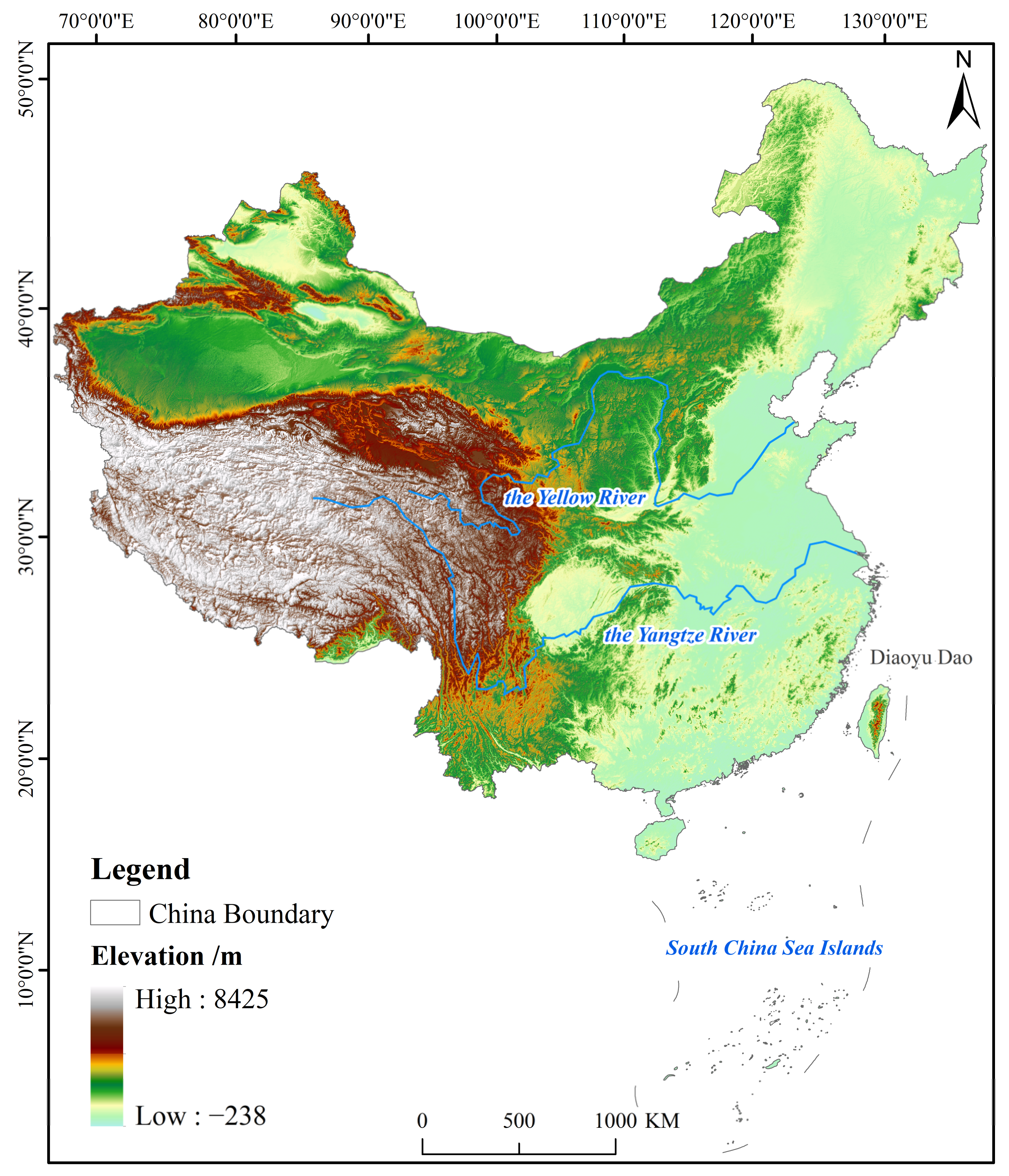
Figure 1. Location of the study area.
Remotesensing 14 00737 g001
Figure 2. Framework of this study.
Remotesensing 14 00737 g002
Figure 3. Spatial distribution and change trend of the RSEI from 2001 to 2020 at different scales. (ae), (gk), (mq) and (sw) display spatial distribution of the RSEI at the county, city, province and urban agglomeration scales, respectively. (f,l,r,x) are change trends of the RSEI at the four scales.
Remotesensing 14 00737 g003
Figure 4. Spatial distribution and change trend of the NTDI from 2001 to 2020 at different scales. (ae), (gk), (mq) and (sw) display the spatial distribution of the NTDI at the county, city, province and urban agglomeration scales, respectively. (f,l,r,x) show the change trend of the NTDI at the four scales.
Remotesensing 14 00737 g004
Figure 5. Spatial distribution and change trend of the MCCD from 2001 to 2020 at different scales. (ae), (gk), (mq) and (sw) display the spatial distribution of the MCCD at the county, city, province and urban agglomeration scales, respectively. (f,l,r,x) show the change trend of the MCCD at four scales.
Remotesensing 14 00737 g005
Figure 6. Global Moran’s I value change trend from 2001 to 2020 at the county scale.
Remotesensing 14 00737 g006
Figure 7. Local Moran’s I spatial distribution of the RSEI, NTDI and MCCD from 2001 to 2020 at the county scale. (ac) display the LISA result of RSEI in 2001, 2010 and 2020. (eg) display the LISA result of NTDI in 2001, 2010 and 2020. (ik) display the LISA result of MCCD in 2001, 2010 and 2020. (d,h,l) indicate local Moran’s I change trends of three indices.
Remotesensing 14 00737 g007
Figure 8. Relationship between the EI and RSEI of Guangdong Province in 2010, 2015 and 2020.
Remotesensing 14 00737 g008
Figure 9. Three-dimensional diagrams of the RSEI, NTDI and MCCD at different scales.
Remotesensing 14 00737 g009
Figure 10. Scatter plots of any two sets of the RSEI, NTDI and MCCD at different scales.
Remotesensing 14 00737 g010
Figure 11. Scatter plot between the original and predicted MCCD at different scales.
Remotesensing 14 00737 g011
Table 1. Introduction of datasets.
NameSpatial and Temporal ResolutionData AvailabilityBrief Description
MOD09A1500 m
8 days
https://lpdaac.usgs.gov/products/mod09a1v006/
accessed on 16 March 2021
A product of surface spectral reflectance of MODIS bands 1–7
MOD11A21000 m
8 days
https://lpdaac.usgs.gov/products/mod11a2v006/
accessed on 19 March 2021
A product of land surface temperature
NPP-VIIRS-like nighttime light data500 m
yearly
https://doi.org/10.7910/DVN/YGIVCD
accessed on 19 March 2021
A nighttime dataset for measuring regional economic development level
WorldPop1000 m
yearly
https://www.worldpop.org
accessed on 23 March 2021
A dataset for measuring population spatial distribution
Administrative division data\http://www.ngcc.cn/ngcc/html/1/index.html
accessed on 5 March 2021
A vector dataset for data clip and spatial analysis
Table 2. Global Moran’s I value at different scales.
Global Moran’s I Value20012005201020152020Change Trend
County ScaleRSEI0.29570.27770.24550.26680.24590.6189
NTDI0.36470.36930.41680.40660.44740.2326
MCCD0.31970.30370.32850.29500.32980.1993
City ScaleRSEI0.32280.30920.27950.27630.24480.5559
NTDI0.27760.30310.31290.34490.38630.3550
MCCD0.28890.30380.29770.31790.34460.2725
Province ScaleRSEI0.13920.08170.06750.09160.05220.2817
NTDI0.25040.27970.28090.24620.33200.1049
MCCD0.26260.29530.28510.21610.27550.0709
Urban Agglomeration ScaleRSEI0.14600.08270.05750.04200.00200.1690
NTDI0.07950.08210.06220.04830.07560.0831
MCCD0.15460.14610.12850.12150.11280.0627
Table 3. Spatial principal component analysis of the RSEI from 2001 to 2020.
EigenvaluePC1PC2PC3PC4
NDVIWETNDBSILSTNDVIWETNDBSILSTNDVIWETNDBSILSTNDVIWETNDBSILST
20010.730.23−0.39−0.500.58−0.31−0.040.74−0.180.76−0.430.440.290.510.810.03
20050.730.24−0.40−0.490.58−0.33−0.030.73−0.170.76−0.410.450.300.490.810.02
20100.750.22−0.41−0.450.55−0.35−0.010.75−0.170.75−0.410.470.310.500.800.02
20150.710.21−0.40−0.520.59−0.29−0.070.74−0.180.77−0.440.410.310.510.790.03
20200.670.25−0.42−0.540.61−0.27−0.130.72−0.230.77−0.420.400.340.510.780.04
Table 4. Fitting formulas of the RSEI, NTDI and MCCD at different scales.
ScaleFitting FormulaAdjusted R2
CountyMCCD = 0.0473 + 0.4521 × RSEI + 0.7831 × NTDI0.8183
CityMCCD = 0.0710 + 0.4574 × RSEI + 0.7576 × NTDI0.9156
ProvinceMCCD = 0.0682 + 0.5053 × RSEI + 0.6441 × NTDI0.9732
Urban agglomerationMCCD = 0.1022 + 0.4595 × RSEI + 0.6561 × NTDI0.9915
Publisher’s Note: MDPI stays neutral with regard to jurisdictional claims in published maps and institutional affiliations.