Assessment of Different Object Detectors for the Maturity Level Classification of Broccoli Crops Using UAV Imagery

Abstract

Broccoli is an example of a high-value crop that requires delicate handling throughout the growing season and during its post-harvesting treatment. As broccoli heads can be easily damaged, they are still harvested by hand. Moreover, human scouting is required to initially identify the field segments where several broccoli plants have reached the desired maturity level, such that they can be harvested while they are in the optimal condition. The aim of this study was to automate this process using state-of-the-art Object Detection architectures trained on georeferenced orthomosaic-derived RGB images captured from low-altitude UAV flights, and to assess their capacity to effectively detect and classify broccoli heads based on their maturity level. The results revealed that the object detection approach for automated maturity classification achieved comparable results to physical scouting overall, especially for the two best-performing architectures, namely Faster R-CNN and CenterNet. Their respective performances were consistently over 80% mAP@50 and 70% mAP@75 when using three levels of maturity, and even higher when simplifying the use case into a two-class problem, exceeding 91% and 83%, respectively. At the same time, geometrical transformations for data augmentations reported improvements, while colour distortions were counterproductive. The best-performing architecture and the trained model could be tested as a prototype in real-time UAV detections in order to assist in on-field broccoli maturity detection.

1. Introduction

The Brassicaceae are a family of flowering plants which are widely known for the multiple health benefits associated with their consumption [1]. Broccoli (Brassica oleracea L. var. italica Plenck.) is one of the most popular crops of this family, the global production of which reached 25 million tons in 2020 (Faostat, 2020). Approximately 10% of this quantity is produced within Europe (Eurostat, 2020, Faostat, 2020). Organic broccoli is an example of a high-value crop that requires delicate handling throughout the growing season and during its post-harvesting handling. In conventional farming, broccoli is mainly harvested mechanically, as the produce is typically intended for the process market (deep freezing). In the case of organic broccoli, as heads can be easily damaged, resulting in visible stains, it is still harvested ‘on sight’ by hand using handheld knives because it is targeted towards the fresh market. On top of that, this allows for a very strict time window of "optimal maturity" when the high-end quality broccoli heads should be harvested, before they remain exposed for too long in high-humidity conditions and become susceptible to fungal infections and quality degradation. Even slight delays from this time window can result in major losses in the final production (Figure 1). However, manual harvesting is a very laborious task, not only for the process of harvesting itself, but for the scouting required to initially identify the field segments where several broccoli plants have reached this maturity level. Moreover, the scouting process is performed on foot, as agricultural vehicles cruising across the fields result in soil compaction, which is highly undesirable in horticulture, especially in the case of organic systems [2].

This case creates a very interesting challenge. First of all, the scouting process can be automated using machine learning, drastically increasing the overall efficiency and reducing the human effort required. At the same time, UAVs can act as a double-benefit factor. They can easily supervise large areas rapidly, whilst diminishing any potential soil-compaction problems. There is a growing need for automated horticultural operations due to increasing uncertainty in the reliability of labour, and to allow for more targeted, data-driven harvesting [3]. To this end, images captured from Unmanned Aerial Vehicles (UAV) could be used to replace the labour work done for field observation. UAVs are widely used in precision agriculture for image capturing and the detection of specific conditions in the field [4]. Compared to the time-consuming work that should be performed by a group of people to find a potential problem in a crop, UAVs could quickly provide a high-resolution image of the field. The produced image, combined with image vision techniques, could output the potential problem/condition that would need to be dealt with [5].

Object detection is a primary field of computer vision, determining the location of certain objects in the image, and then classifying those objects [6]. Initially, the first methods used to address this problem consisted of two stages: (1) the Feature Extraction stage, in which different areas in the image are identified using sliding windows of different sizes, and (2) the Classification stage, in which the classes of the objects detected are estimated. A common method for the implementation of image classification is the sliding window approach, where the classifier runs at evenly spaced locations over the entire image. Object detection algorithms are evaluated based on the speed and the accuracy that are demonstrated, but their optimisation in both factors could be a very challenging task [6].

Object detection techniques apply classifiers or localizers to perform detections on images at multiple locations and scales. Recent approaches like the R-CNN and its variations use region proposal methods to generate, initially, several potential bounding boxes across the image, and then run the classifier on these proposed boxes. During training with those approaches, after every classification, post-processing steps are used to refine the bounding boxes, usually by increasing the score of the best-performed bounding boxes and decreasing the worse ones, ultimately eliminating potential duplicate detections [7]. Faster R-CNN [8] is one of the most widely used two-stage object detectors. The first stage uses a region proposal network, which is an attention mechanism developed as an alternative to the earlier sliding window-based approaches. In the second stage, bounding box regression and object classification are performed. Faster R-CNN is fairly well-recognized as a successful architecture for object detection, but it is not the only meta-architecture which is able to reach state-of-the-art results [9]. On the other hand, single-shot detectors, such as SSD [10] and RetinaNet [11], integrate the entire object detection process into a single neural network to generate each bounding box prediction.

Automation in agriculture presents a more challenging situation compared to industrial automation due to field conditions and the outdoor environment in general [12,13]. Fundamentally, most tasks demand a high accuracy of crop detection and localization, as they are both critical components for any automated task in agriculture [14]. The fact that there is a constant downward trend of the available agricultural labour force [15] also adds to this problem, and makes the automation of several production aspects a necessity. Accurate crop detection and classification are essential for several applications [5], including crop/fruit counting and yield estimation. Crop detection is often the preliminary step, followed by the classification operation, such as the quantification of the infestation level through the identification of disease symptoms [16], or as per the subject of the present paper, maturity detection for the automation of crop surveying. At the same time, it is the single most crucial component for automated real-time actuation tasks, such as automated targeted spraying applications or robotic harvesting.

Focusing on horticultural crops, automation in growth-stage identification has been an open challenge for multiple decades due to the very nature of the crops, which in their majority are high-value and demand timely interventions to maintain top-cut yield quality. Therefore, different approaches have been implemented to achieve the automated mapping of crop growth across larger fields and to assist harvesting, either by correlating the images’ frequency bands with broccoli head sizes for maturity detection [17,18,19] or to combine image analysis techniques and neural networks to identify broccoli quality parameters [20].

As developments in computer vision allowed the research to move from simple image analysis frameworks to more complex and automated pipelines, the interest shifted towards Artificial Intelligence. Commercial RGB cameras and machine learning algorithms can provide affordable and versatile solutions for crop detection. Computer vision systems based on deep CNN [21] are immune to variations in illumination and large inter-class variability [22], both of which have posed challenges in agricultural imaging in the past, thus achieving the robust recognition of the targets in open-field conditions. Recent research [23,24,25] have shown that the Faster R-CNN (region-based convolutional neural network) architecture [8,26] or different YOLO model versions [27,28,29] can produce accurate results for a large set of horticultural crops and fruit orchards. Moreover, a comparison of different computer vision techniques, such as object detection and object segmentation [30], has provided significant improvements in crop detection. In recent horticultural research literature, several studies have also focused on the localization of broccoli heads, without any evaluation of their maturity, by implementing deep learning techniques [31,32,33,34].

The objective of this study was to compare state-of-the-art object detection architectures and data augmentation techniques, and to assess their potential in the maturity classification of open-field broccoli crops, using a high-Ground Sampling Distance (GSD) RGB image dataset collected from low-altitude UAV flights. The best-performing architecture and the trained model could be tested as a prototype in real-time UAV detections in order to assist in on-field broccoli maturity detection.

2. Materials and Methods

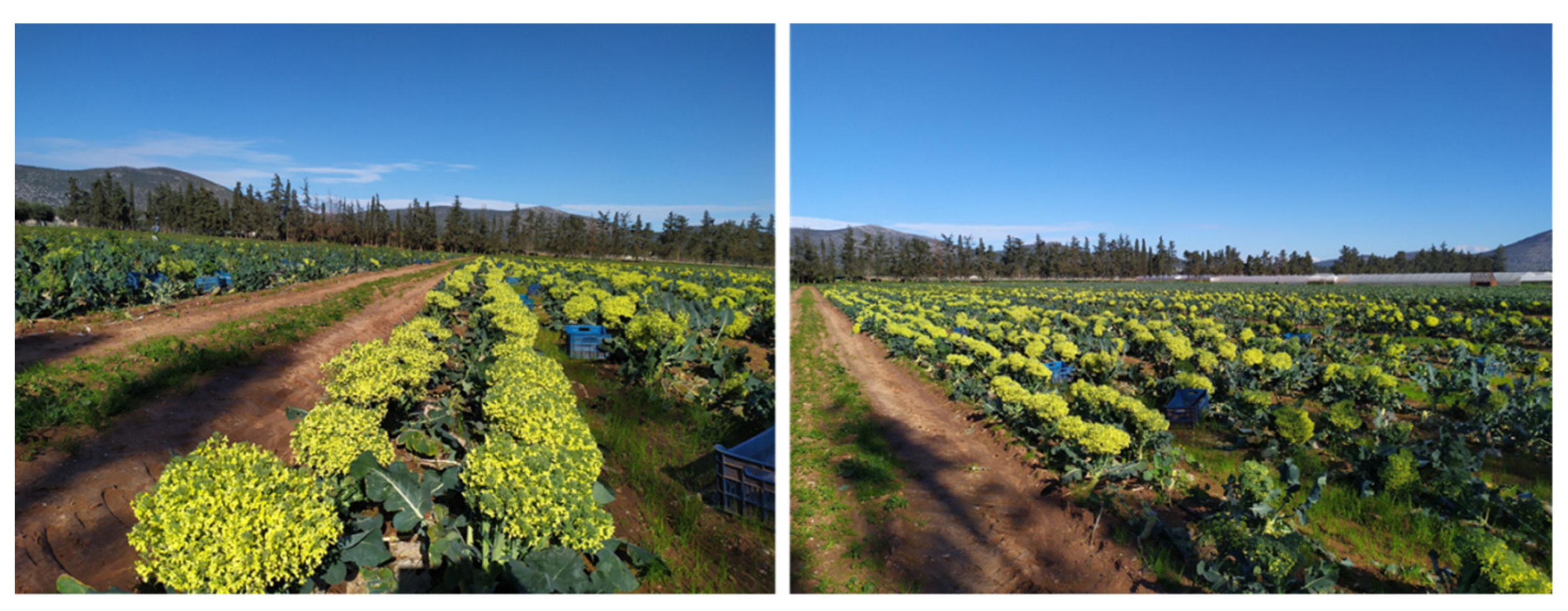
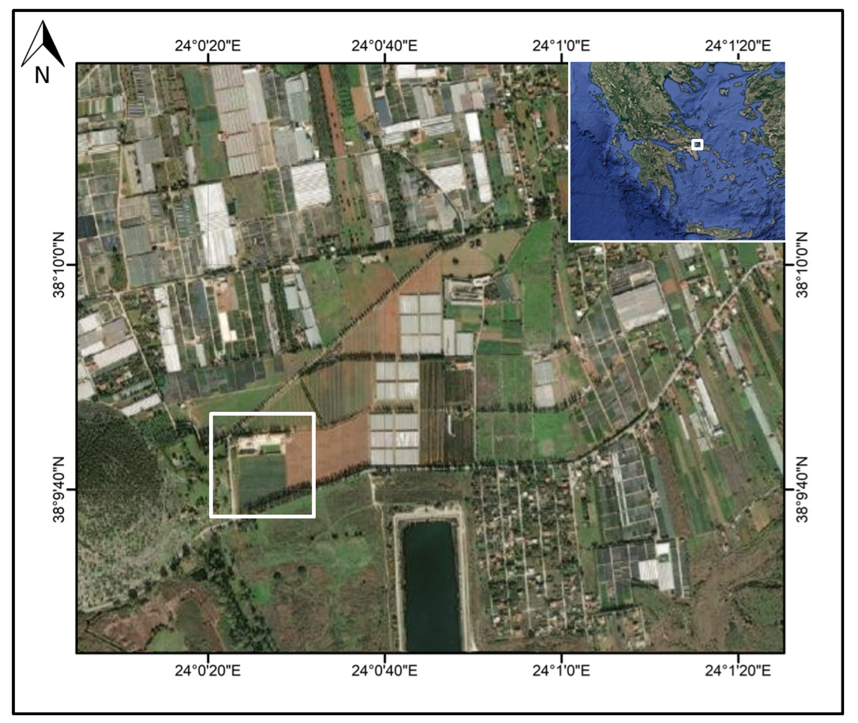
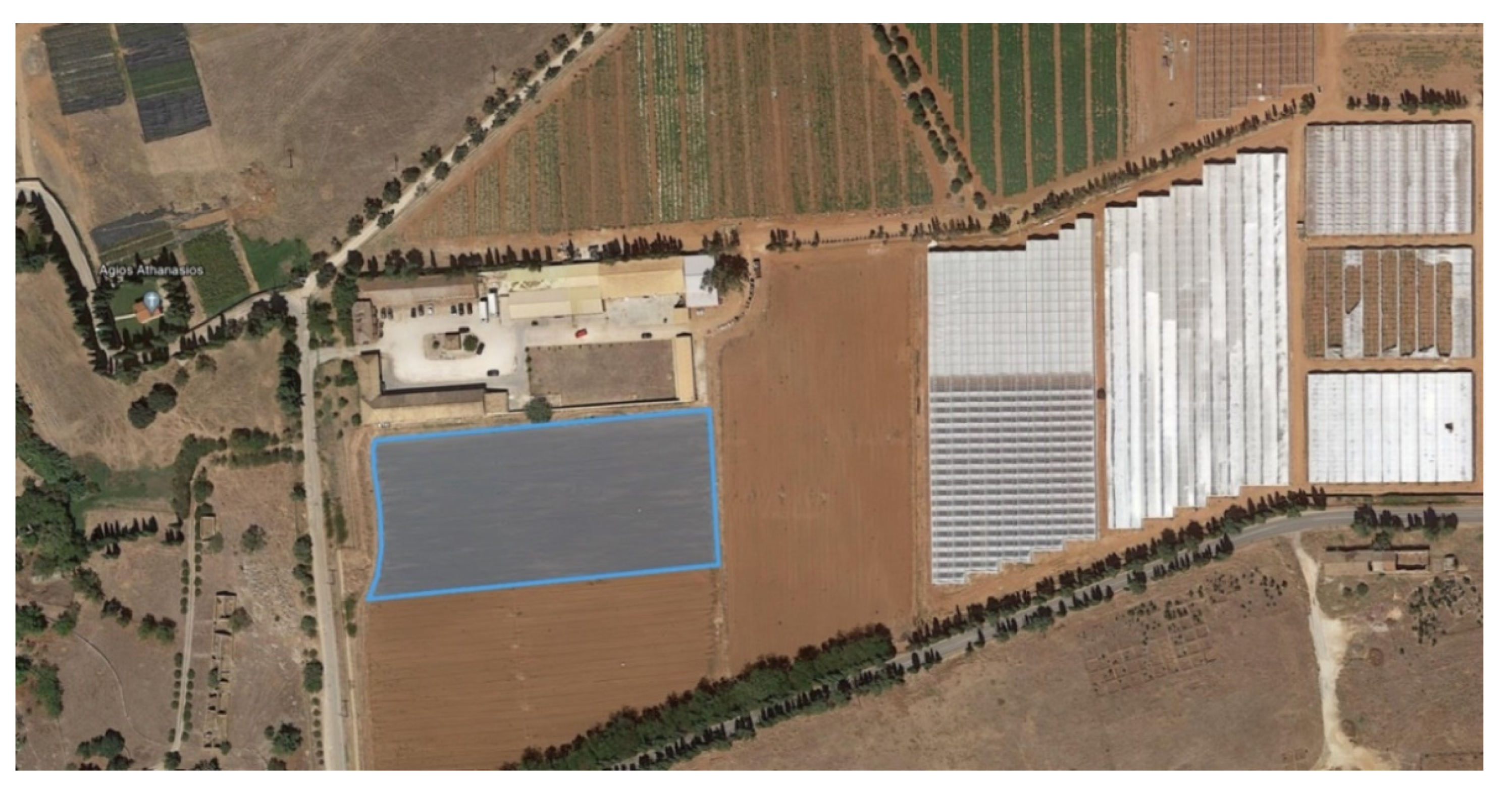
2.1. Experimental Location

The experiment took place in Marathon, Greece (42 km north from Athens), in a commercial organic vegetable production unit (Megafarm Gaia mas). This region is specifically known for its horticultural production, being the main vegetable provider for Athens. The timing of the data acquisition flights was specifically designed to be performed a few hours prior to the first wave of selective harvesting. This was desired for two reasons: (1) to ensure that the entire field was intact (no broccoli heads were harvested), maximising the sample density in every image and the generated field orthomosaic; and (2) to make sure that individual plants of different maturity levels were present across the field, as it was at the very start of the harvesting season. The selected experimental parcel was located in the south-west part of the production unit, and occupied an area of approximately 1 ha. The segment on which the ground truth targets were deployed covered slightly more than half of it (Figure 2 and Figure 3).

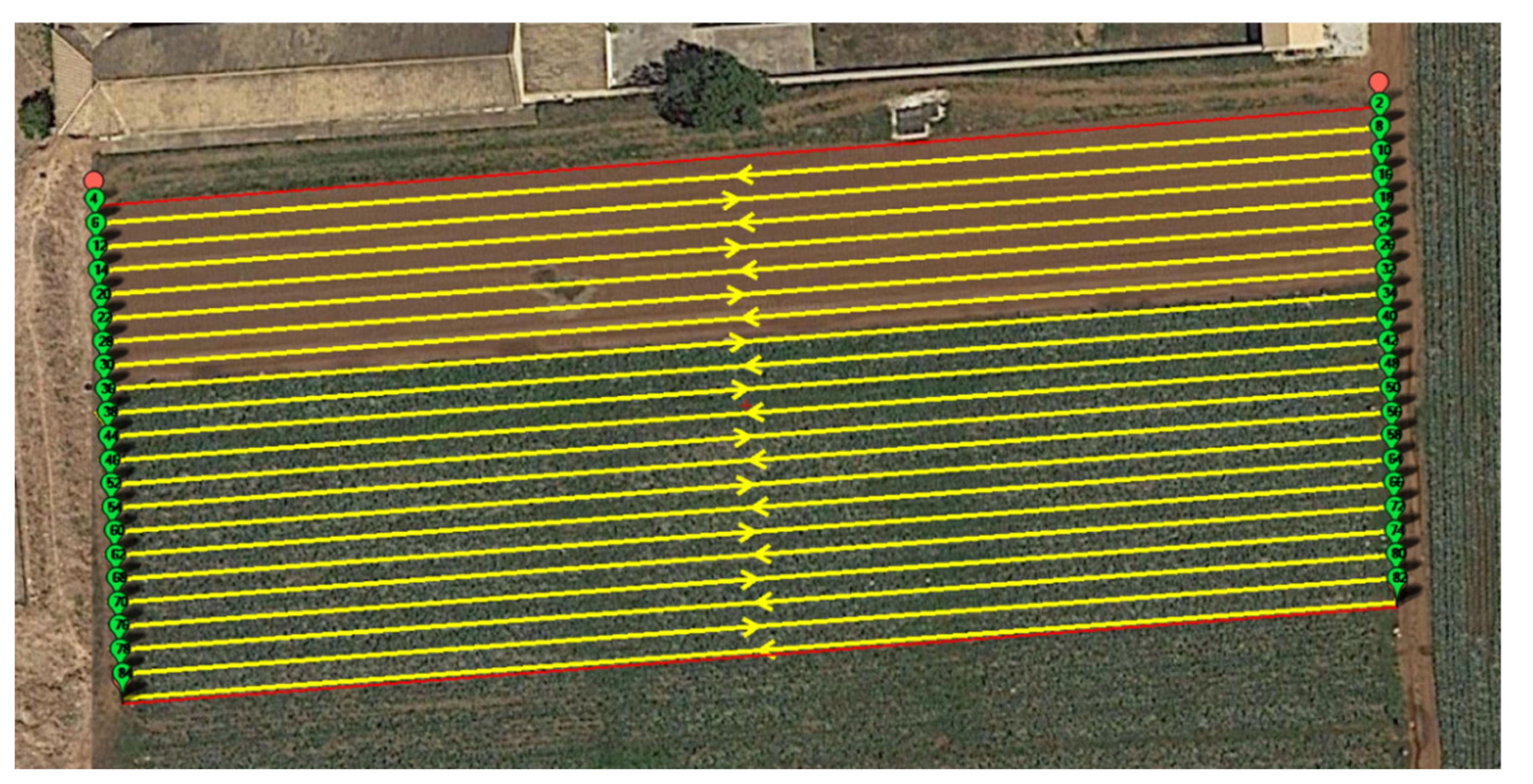
2.2. Data Acquisition

The data collection was performed by a custom quadcopter drone equipped with a 20-megapixel (4096 × 2160 resolution) CMOS mechanical shutter RGB camera, which was used to generate the low-altitude aerial imagery dataset. The images were captured and saved in the 16-bit JPG format, accompanied by the georeferencing metadata of each image. A total of 3 flight missions were executed during the time window between 11:00 and 13:00 (when the solar elevation angle was greater than 45°), in order to avoid drastic deviations in solar illumination between the flights. The flights were executed with similar flight parameters across all of the flights, operating at a fixed altitude of 10 m AGL ±0.5 m (GPS vertical hovering error), which is considered to be consistent towards the ground because the field was levelled by a flattening cultivation roller approximately 4 months prior to the measurements. The sensor was set to capture images at a fixed interval of 2 sec/capture, and therefore the flight plans were designed around this parameter. The frontal and lateral overlaps were both selected to be 80%, resulting in a cruising speed of approximately 1.1 m/s. Finally, the orientation of the flight lines was selected to be parallel to the orientation of the planting rows. The generated flight plan is also presented below (Figure 4), and was executed three times consecutively by the UAV.

Before the start of the data collection flights, a total of 45 ground truth targets were deployed and stabilised across the field, in order to support the annotation stage (described in the following section). The targets indicated the maturity level of the selected broccoli crops, as they were categorised by an expert agronomist who participated in the process. The human expert indicated a total of 15 broccoli heads of 3 different broccoli maturity classes. These classes ranged from 1 to 3, with class 1 representing immature crops that would not be harvested for at least the following 15 days, class 2 representing heads that are estimated to reach harvesting level within a week, and finally, class 3, which contained exclusively “ready to harvest” heads. Due to the high humidity of the air near the surface and the constantly wet soil, the targets were enveloped inside transparent plastic cases in order to protect them from decomposing, as they would remain on the field for approximately two hours. The cases had been tested in the university campus to verify that the labels (numbering) remained visible in the UAV imagery. In case a ground truth label was covered heavily by the surrounding leaves, a bright-yellow point-like object was also placed nearby as a pointer. Examples of the deployed targets are presented below (Figure 5).

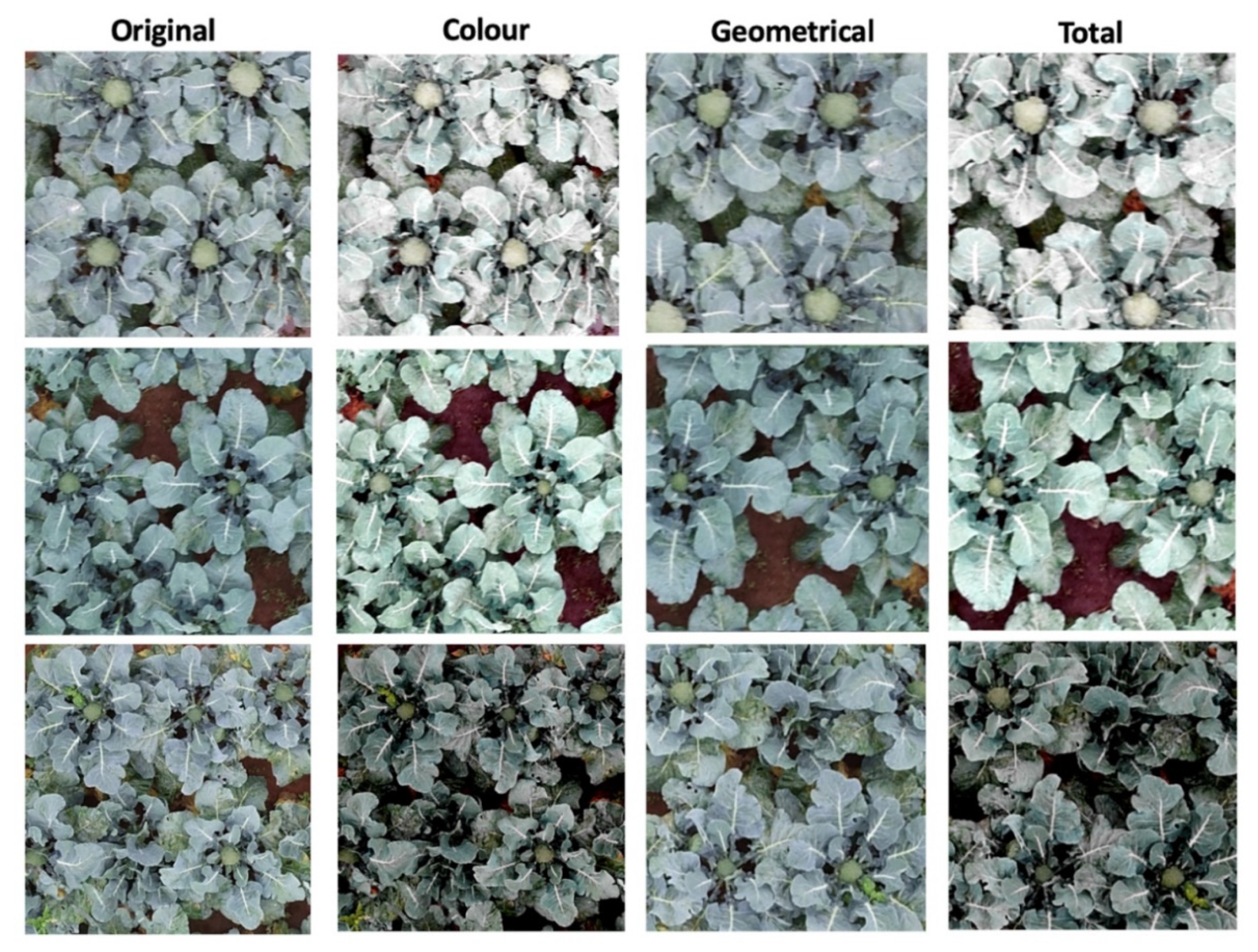
2.3. Data Pre-Processing

Following the field data acquisition by the UAV and the imaging components, data pre-processing was performed in remote computational units. The first step of the data processing phase was to generate the orthomosaic maps from each flight. For this process, the photogrammetric software Pix4D Mapper (Pix4D SA) was used, generating a total of three (3) RGB orthomosaics, with a final GSD of 0.25 cm. In the following step, the single best orthomosaic was selected in order to ensure that the final dataset that was going to be presented to the machine did not contain duplicates of the same crops, as this would increase the initial bias of the experiment. After close inspection, the mosaic of the second flight was selected, as it produced an orthomosaic of slightly higher quality (less blurry spots and zero holes), potentially indicating that the flight conditions were better during that time window, which enabled the UAV to perform its flight in a more optimal way with fewer disruptions.

Once the mosaic was selected, the next step was to create the dataset that would be fed to the models. As the generated mosaic was georeferenced, an initial crop with a vector layer was performed in a GIS (QGIS 3.10) to eliminate the majority of the black, zero-valued pixels that were created during the mosaicking process (the exported mosaic is written in a minimum-bounding-box method, surrounding the mosaic map with black pixels to create a rectangle, were all of the bands are assigned a zero value for the pixels which did not contain any data). This cropping served another purpose, as the next pre-processing step involved “cutting” the mosaics into smaller images so that they could be used as an input for the models. This was easily performed using a script written in Python that iterated the entire mosaic and then copied the first X number of pixels in one direction and Y pixels in the other direction for all of the bands of the initial mosaic. In our case, the desired image dimensions were 500 × 500 pixels, and therefore the step of each loop (one for each axis, as the rectangular mosaic is scanned) was set to 500, to result in a dataset of rectangular RGB images with a uniform resolution.

The final step of the pre-processing involved object labelling on individual images. In this phase, the generated dataset was imported to the Computer Vision Annotation Tool (CVAT), and the images were annotated using the ground truth labels as a basis (Figure 4). Finally, the annotations of the dataset were exported in the PASCAL Visual Object Classes (VOC) format [35], as this format of bounding box annotations is required by Tensorflow. PASCAL VOC is an XML annotation format that requires a pixel-positioning encoding, meaning that once drawn, each annotation file is exported in the form of a text file containing the sequence of the four coordinates of each bounding box within the image. The annotations consisted of rectangular boxes assigned with the respective maturity class of each broccoli head they contained. The final dataset contained a total of 288 images with over 640 annotations, where most of the bounding boxes presented a squared shape (Figure 6).

2.4. Object Detection Pipelines

In order to create robust object detectors which are still reliable on test images, usually, it is necessary to use a training pipeline where implicit regularization, such as data augmentation, is applied during the training process without constraining the model capacity. Data augmentation in computer vision is a set of techniques performed on the original images to increase the number of images seen by the model while training. As studied in several works [36,37], having the right data augmentation pipeline is critical in order for agricultural computer vision systems to work effectively. As shown in Figure 7, the two particular augmentation transforms that seem to have the most impact are (i) geometrical transformations and (ii) colour distortions. In this work, in the geometrical augmentation approach, horizontal and vertical flipping, and random cropping with resizing were implemented. With regard to the colour distortion, slight modifications in the brightness, contrast, hue and saturation were implemented. All of the data augmentations were executed with a probability of 50%.

Several object detectors have arisen in the last few years, with each of them having different advantages and disadvantages. Some of them are faster and less accurate, while others have higher performances but use more computational resources, which sometimes are not suitable depending on the deployment platform. In this work, five different object detectors were used: Faster R-CNN [8], SSD [10], CenterNet [38], RetinaNet [11] and EfficientDet-D1 [39].

Table 1. The selected object detection architectures used for the experiment.

Object Detector	Backbone	Input Size	FPN	COCO mAP
Faster R-CNN	ResNet-152	640 × 640	No	32.4
SSD	MobileNet-V2	640 × 640	Yes	28.2
RetinaNet	ResNet-152	640 × 640	Yes	35.4
EfficientDet-D1	EfficientNet-D1	640 × 640	Yes	38.4
CenterNet	HG-104	512 × 512	No	41.9

shows the specific detectors evaluated in this work. Except for the input size, the value of which was the closest to the original image size (500 × 500), the most promising ones were selected after some early experiments. It can be observed that ResNet-152 [22] is used as the backbone in two object detectors (Faster R-CNN and RetinaNet). Furthermore, HourGlass-104 [40], MobileNet-V2 [41] and EfficientNet-D1 [39] were evaluated. On the other hand, three of them use a Feature-Pyramid-Network (FPN), which is supposed to provide better performance in the detection of small objects. The reason for selecting these architectures is that different detection “families” are represented. For instance, SSD (e.g.: RetinaNet) and two-shot (Faster R-CNN) were compared in order to verify that the second one may lead to better performances than the basic approach (SSD and MobileNet-V2). However, the architectural improvements of RetinaNet (e.g., focal loss) could invert this assumption. On the other hand, the inference time was out of the scope of this paper, in which real-time detection is not discussed; however, theoretically, SSD could lead to faster inferences. Additionally, with these detectors, the anchorless approach was contrasted against the traditional anchor-based detection. Again, the most important theoretical gain could be the inference time, which is not discussed; however, related works presented the promising performances of CenterNet, which could be the chosen detector for future deployment on the field. Table 1 also reports the mAP (mean Average Precision) obtained on the COCO dataset. From this performance, it can be estimated that CenterNet and EfficientDet-D1 will be the best detectors, while SSD (MobileNet) and Faster R-CNN will be the least promising ones.

When developing an object detection pipeline, it is important to fine-tune different hyper-parameters in order to select the ones that better fit a specific dataset. This means that different datasets could lead to different hyper-parameter configurations in every detector.

Table 2. Hyper-parameters evaluated for each detector.

Hyper-Parameter	Values
Optimizer	{Adam, SGD}
Learning Rate (LR)	{0.05, 0.01, 0.001}
Batch Size	{4, 8}
Warmup steps	{100, 500, 1000}
IoU Threshold	{0.1, 0.25, 0.5}
Max. Detections	{10, 50, 100}

presents the evaluated hyper-parameter space used in this work to choose the most promising ones after 5 runs with different train-validations-test splits (see

Table 3. Hyper-parameters selected for the final experiments.

Object Detector	Optimizer	LR	Batch Size	Warmup Steps	IoU Threshold	Max. Detections
Faster R-CNN	SGD	0.05	4	500	0.5	100
SSD	SGD	0.01	8	1000	0.25	100
RetinaNet	SGD	0.01	8	100	0.25	50
EfficientDet-D1	SGD	0.04	4	500	0.5	50
CenterNet	Adam	0.001	8	1000	-	-

). The selected configurations were executed for 5 additional runs in order to complete the experimental trials and extract some statistics.

Two different optimizers were evaluated: Adam and SGD. All of the detectors performed better with SGD except CenterNet, which obtained its best performances with Adam. Related to the optimizer, the learning rate (LR) also played a major role. Adam worked better with the smallest evaluated LR (0.001), while SGD obtained the best performance with higher LRs (0.05 and 0.01). Two additional hyper-parameters that completely changed the training behavior were the warmup steps and the batch size. The warmup is the period of the training where the LR starts small and smoothly increases until it reaches the selected LR (0.05, 0.01 or 0.001). Every detector needed a different combination to obtain their best performance, but it is important to remark that the use of less than 500 steps (around 10 epochs) for warming obtained poor performances. Finally, all of the detectors, except CenterNet, which uses an anchorless approach, needed to run the Non-Maximum-Suppression (NMS) algorithm to remove redundant detections of the same object. Two important values configure this algorithm: the ratio to consider that two predicted bounding boxes point to the same object (the IoU threshold in the tables) and the maximum number of detections allowed (the Max. detections in the tables). As can be observed, again, all of the detectors found a different combination as the most promising one, which are presented in Table 3. Finally, an early stopping technique to avoid overfitting was implemented. Specifically, if the difference between the training and validation performances is greater than 5% for 10 epochs, the training process stops. All of the detectors were trained for a maximum of 50 epochs.

In this work, the experiments were carried out with GeForce RTX 3090 GPU under Ubuntu 18.04. For the software, Tensorflow 2.6.0 was used to implement the object detector pipelines. Early experiments to gain knowledge on the most promising detectors were implemented through parallel tasks in an HPC cluster (ARIS infrastructure https://hpc.grnet.gr/en/, accessed date: 13 January 2022) with 2 NVIDIA V100 GPU cards.

2.5. Evaluation Metrics

Because comparing the results of different architectures is not trivial, several benchmarks were developed and updated over the last few years for detection challenges, and different researchers may evaluate their model’s skills on different benchmarks. In this paper, the evaluation method for the broccoli maturity detection task was based on the Microsoft COCO: Common Objects in Context dataset [42], which is probably the most commonly used dataset for object detection in images. Like COCO, the results of the broccoli maturity detection were reported using the Average Precision (AP). Precision is defined as the number of true positives divided by the sum of true positives (TP) and false positives (FP), while AP is the precision averaged across all of the unique recall levels. Because the calculation of AP only involves one class and, in object detection, there are usually several classes (3 in this paper), the mean Average Precision (mAP) is defined as the mean of the AP across all classes. In order to decide what a TP is, the Intersection over Union (IoU) threshold was used. IoU is defined as the area of the intersection divided by the area of the union of a predicted bounding box. For example, Figure 8 shows different IoUs in the same image and ground truth (red box) by varying the prediction (yellow box). If an IoU > 0.5 is configured, only the third image will contain a TP, while the other two will contain an FP. On the other hand, if an IoU > 0.4 is used, the central image will also count as a TP. In case multiple predictions correspond to the same ground truth, only the one with the highest IoU counts as a TP, while the remaining are considered FPs. Specifically, COCO reports the AP for two detection thresholds: IoU > 0.5 (traditional) and IoU > 0.75 (strict), which are the same thresholds used in this work. Additionally, the mAP with small objects (area less than 32 × 32 pixels) was also reported.

3. Results

The experiment results were obtained by averaging 10 different trials for each individual architecture. In each case, a stratified split was performed, with 70% of the samples being used for training, 10% of the samples being used for validation, and 20% of the samples being used for testing. Besides the performances on the test set, all of the tables include the mAP@50 on the training set, in order to illustrate the chances of overfitting.

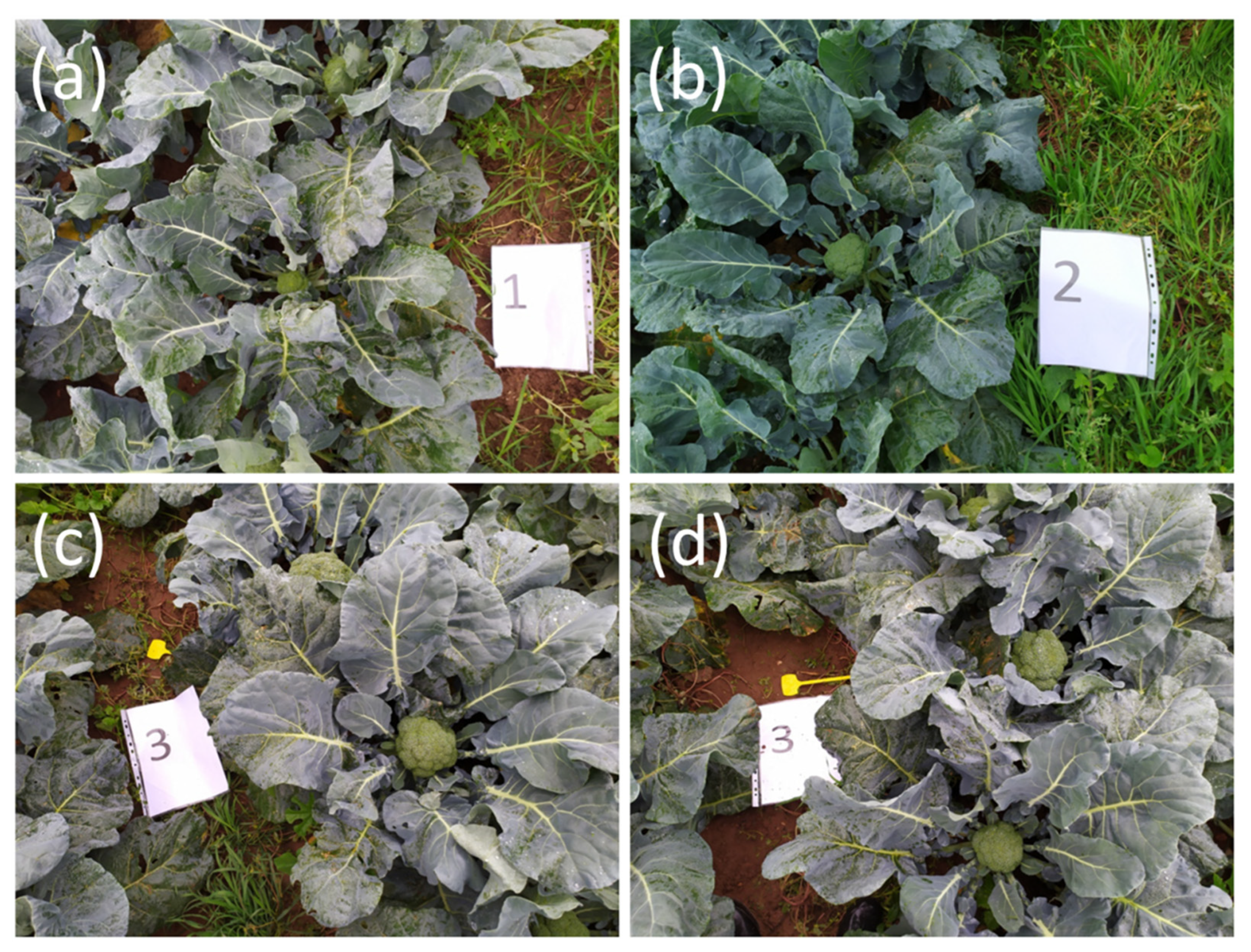
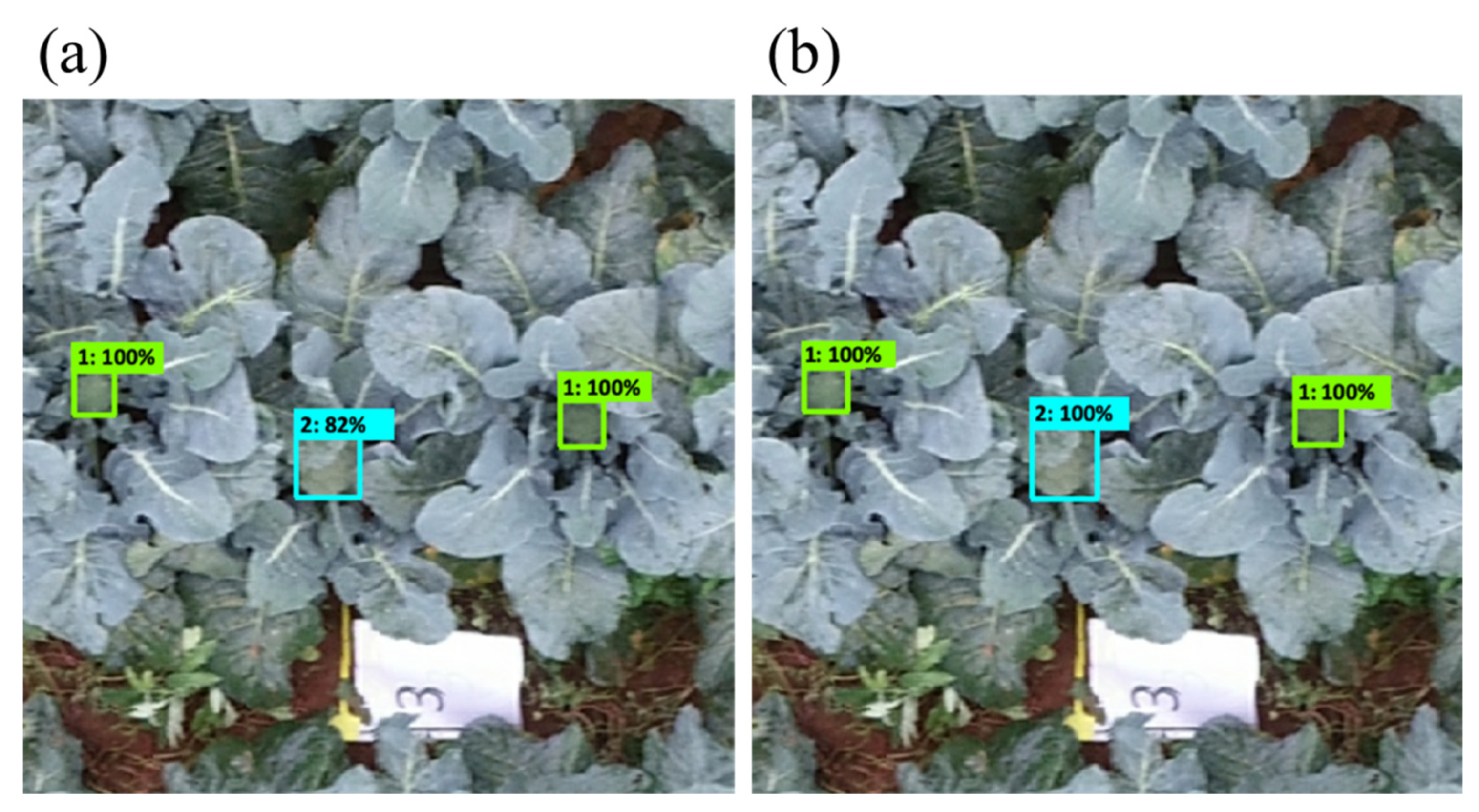
3.1. Three-Class Approach

The performance of each architecture without using any type of data augmentation is shown in

Table 4. The performance of each architecture without any data augmentation techniques. In the parentheses, the training performance is presented for mAP@50. The bold numbers correspond to the best performances.

Object Detector	mAP@50	mAP@75	mAP@small
Faster R-CNN (ResNet)	82.6 ± 4.13 (86.3)	71.1 ± 4.01	54.66 ± 9.16
CenterNet	80.43 ± 2.46 (79.15)	73.24 ± 2.81	57.05 ± 8.66
SSD (MobileNet)	78.89 ± 3.69 (82.13)	69.1 ± 3.84	44.85 ± 8.75
RetinaNet	78.36 ± 1.84 (81.48)	62.24 ± 3.3	48.09 ± 6.01
EfficientDet-D1	77.68 ± 3.48 (79.16)	65.94 ± 4.22	48.85 ± 7.9

. As can be observed, Faster R-CNN (ResNet) is the object detector that showed the highest mAP@50 on average; however, it was not the case for mAP@75 and the performance with small objects, for which CenterNet performed better. SSD-MobileNet, RetinaNet and EfficientDet-D1 all demonstrated a lower performance, especially in the detection of small objects.

In the following step, a single form of augmentation was used at a time, and all of the architectures were evaluated in a similar process.

Table 5. The performance of each architecture with only geometric augmentation active. In the parentheses, the training performance is presented for mAP@50.

Object Detector	mAP@50	mAP@75	mAP@small
Faster R-CNN (ResNet)	84.19 ± 2.96 (83.12)	73.6 ± 3.17	60.09 ± 7.78
CenterNet	83.68 ± 1.17 (85.18)	75.59 ± 1.47	59.39 ± 4.31
SSD (MobileNet)	82.81 ± 2.2 (81.36)	73.92 ± 2.1	59.17 ± 7.87
EfficientDet-D1	82.76 ± 2.56 (82.45)	71.91 ± 3.2	57.58 ± 7.89
RetinaNet	79.53 ± 3.21 (78.95)	65.44 ± 6.59	55.75 ± 5.8

shows the performances when using geometrical augmentations. The performances improved in all of the cases. Faster R-CNN (ResNet) and CenterNet obtained the best results in mAP@50, mAP@75 and mAP@small. However, in this case, Faster R-CNN (ResNet) ranked first in the detection of small objects.

Table 6. The performance of each architecture with only colour augmentation active. In the parentheses, the training performance is presented for mAP@50. The bold numbers correspond to the best performances.

Object Detector	mAP@50	mAP@75	mAP@small
Faster R-CNN (ResNet)	83.17 ± 2.72 (84.16)	73.52 ± 2.09	58.42 ± 6
CenterNet	80.82 ± 2.7 (81.33)	77.17 ± 2.82	55.75 ± 6.21
EfficientDet-D1	79 ± 2.01 (80.47)	65.71 ± 2.97	52.44 ± 7.27
RetinaNet	77.45 ± 2.52 (76.74)	63.24 ± 3.91	46.18 ± 12.16
SSD (MobileNet)	77.38 ± 2.7 (76.49)	68.44 ± 3.2	45.4 ± 5.66

shows the performances when using only colour augmentations. Similarly to the previous configurations, Faster R-CNN (ResNet) and CenterNet obtained the best performances. The bold numbers correspond to the best performances.

Table 7. The performance of each architecture with both augmentation types (geometrical and colour) active. In the parentheses, the training performance is presented for mAP@50. The bold numbers correspond to the best performances.

Object Detector	mAP@50	mAP@75	mAP@small
CenterNet	83.52 ± 1.57 (85.98)	79.53 ± 1.54	59.73 ± 6.92
RetinaNet	83.28 ± 1.83 (84.17)	71.6 ± 2.15	61.22 ± 5.21
EfficientDet-D1	83.02 ± 1.44 (82.63)	72.73 ± 3.22	58.24 ± 5.29
SSD (MobileNet)	82.56 ± 3.18 (81.92)	72.14 ± 3.27	59.3 ± 7.51
Faster R-CNN (ResNet)	82.52 ± 4.32 (85.17)	70.96 ± 5.92	56.04 ± 8.17

shows the performances when using both colour and geometrical augmentations at the same time. In general, all of the architectures improved their mAP@50 except for Faster R-CNN (ResNet), the performance of which remained similar. As in the previous experiments, CenterNet was the best detector according to mAP@75 (besides mAP@50), confirming its superiority when giving accurate locations.

Figure 9 depicts a box plot summarizing the performance of the detectors across all of the data augmentations. As can be inferred from the previous tables, Faster RCNN and CenterNet are the most consistent detectors at mAP@50 and mAP@75. However, both architectures presented a different behavior at the same time. On the one hand, Faster RCNN was able to obtain the highest performances with a higher variance. On the other hand, CenterNet did not reach the maximum, but showed more consistent performance. The other detectors (SSD, EfficientDet-D1 and RetinaNet) performed worse on average, but in some specific experiments, they were able to reach higher mAPs than CenterNet.

In order to provide a better description of how the data augmentation stage performs in the detection pipelines, Figure 10 depicts how each augmentation method has worked across all of the experiments and detectors. It can be observed that, in general, geometrical augmentation and complete augmentation show the higher median; however, with mAP@50, complete augmentation shows a more dispersed distribution, making it a less reliable augmentation. On the other hand, with mAP@75, geometrical augmentation obtains a more clear superiority over the rest of the detectors. Finally, Figure 10 also shows that all of the types of augmentations can reach the maximum performances (around 87.5%) with mAP@50, and close to maximum—obtained by geometrical augmentation—with mAP@75.

3.2. Two-Class Approach

Regarding the performance for each individual maturity class, as observed in our results, the highest performing class was maturity class 3, followed by class 2, and finally class 1. Most class-3 broccoli heads were both detected successfully and classified correctly. In the case of lower maturity classes (1 and 2), despite the fact that the broccoli heads were distinguishable and thus correctly detected as objects, they would often be mixed between them in the classification step, as the architectures could not always tell them apart, and thus misclassified them. An example of this instance is presented in Figure 11, in which the single class-3 broccoli head present in the image was detected and classified correctly, while two class-2 heads, although properly detected, were misclassified as class 1.

These observations led us to speculate that the architectures would potentially yield even better results and demonstrate a stronger performance if the problem presented was a simplified “ready to harvest” and “not ready yet” two-class problem. In order to test this hypothesis, the two best- and the two worst-performing pipelines (based on both data augmentation and architecture) were selected and evaluated on the two-class version of the dataset, where maturity classes 1 and 2 were merged into a single class, while class 3 was kept intact.

Table 8. The performance of the selected architectures and augmentation types on the two-class dataset. In the parentheses, the training performance is presented for mAP@50. The bold numbers correspond to the best performances.

Pipeline	mAP@50	mAP@75	mAP@small
Geometrical + CenterNet	83.52 ± 1.57 (84.79)	79.53 ± 1.54	59.73 ± 6.92
Geometrical + Faster R-CNN (ResNet)	83.28 ± 1.83 (82.85)	71.6 ± 2.15	61.22 ± 5.21
Colour + SSD (MobileNet)	83.02 ± 1.44 (86.19)	72.73 ± 3.22	58.24 ± 5.29
Colour + RetinaNet	82.56 ± 3.18 (82.50)	72.14 ± 3.27	59.3 ± 7.51

presents the performances of the four selected pipelines once the problem was simplified from three classes to two classes. As can be observed, all of the performances improved while the ranking of the pipelines was the expected. Finally, a similar detection example using the two-class approach, on the same image as Figure 11, is shown in Figure 12.

4. Discussion

The results have shown that, across all of the experiments, Faster R-CNN and CenterNet were the best-performing architectures for the task of broccoli maturity detection (Table 4, Table 5, Table 6 and Table 7, and Figure 9). Their performances were, on average, always over 80% for mAP@50 and 70% for mAP@75 in the three-class problem, regardless of the hyperparameter configuration and augmentation techniques, which were solid performances considering the open-field nature of the dataset. The same pattern was encountered in the detection of small objects. Nonetheless, it is important to note that the differences were too small with high standard deviations, making it difficult to claim the best detector with small objects. According to Table 1, the high performance of CenterNet was expected due to its highest mAP on the COCO dataset in comparison to the other detectors. However, Faster R-CNN was, in theory, less promising than more recent architectures such as EfficientDet-D1 and RetinaNet. Additionally, Faster R-CNN and RetinaNet shared the same backbone, which made the comparison closer to the single-shot against two-shot detectors. In this case, the two-shot approach surpassed both SSD methods. This result highlights the fact that the evaluation of old architectures on new domains is always a worthy task, and opens the question of whether SSD may need deeper backbone architectures (e.g., ResNet 164) in order to consistently overcome the two-shot approach. This experiment could be carried out because the inference time in SSD is lower, and it could be increased by a deeper backbone to match the Faster R-CNN’s times and performances. However, this approach could have a limit because embedded systems where the detector would be deployed have hardware limitations, and smaller architectures such as MobileNet would be preferable. However, according to the poor results shown in this work by MobileNet V2, the version 3 (both small and large) architectures should be evaluated to throw some light on this problem.

Another important aspect of this research was to evaluate different data augmentation approaches due to the relevance that this technique currently has in related literature. Without any form of augmentation, the best-performing architectures were Faster R-CNN (ResNet) for mAP@50 and CenterNet for mAP@75, achieving over 82% and 73%, respectively (Table 4). However, as it was hypothesized, not using augmentations did not obtain the best performances. Moreover, as can be observed in the presented tables, augmentation made the difference between training and testing lower, which can be translated into lower chances of overfitting. Focusing on the most promising augmentation techniques, geometrical techniques with and without the combination of colour distortions led to the highest performances overall (see Figure 10). By using only geometrical augmentation, Faster R-CNN (ResNet) managed to score the highest mAP@50 across all of the configurations and architectures (84.19%). On the other hand, it was quite remarkable that colour distortion by itself decreased the performance. For example, SSD-MobileNet decreased its mAP@50 from 78.89% (non-augmentation) and 82.82% (geometrical augmentation) to 77.38% (colour augmentation). Finally, with both colour and geometrical augmentations active, a surprising result was the improvement of RetinaNet, which not only obtained the second-best performance across all of the architectures but also achieved the highest mAP@small across all of the architectures and augmentation configurations. In addition, Faster R-CNN (ResNet) performed worse than the use of a single form of augmentation (colour and geometrical) separately.

The improvement of the geometrical augmentation is aligned with the results presented in [31,43], although the specific transformations were different. As discussed by these authors, these geometrically transformed images are similar to broccoli from the test set because the test images also contain broccolis of different sizes, scales, and positions. As a result, these transformed images allowed the neural network to better generalize, and to detect the broccolis in the test images with a higher mAP. However, with the colour transformations, the transformed images were less similar to the broccolis of the test set. Some unrealistic dark or bright images could appear, and even changes in textures that differed from the textural patterns learned while training could result in a lower mAP (See Figure 7). Moreover, this can lead to the conclusion that the use of standard augmentations, which usually work in popular datasets like COCO, could not work in some specific domains like agriculture and maturity level classification, where colour plays an important role. Another relevant remark for data augmentation is that all of the types of augmentation were able to reach performances of around 87.5% in some specific train–test splits and pipeline configurations. This reinforces the need to run several experiments with different splits in order to deeply understand the general behaviour of a specific detection pipeline.

For the two-class approach, the performance was significantly higher for the tested detectors, indicating that the merging of the two lower-maturity classes into one, and essentially only separating them from ready-to-harvest plants, was successful. This is another logical outcome considering that the “boundaries” between the classes were an approximation method for field labelling, and not an actual measurable metric. As a result, some level of confusion might occur even for a human observer tasked to separate the instances of these two classes. From an agronomic point of view, quantifying maturity in the early stages holds some value regarding the early planning of upcoming harvesting operations. Nevertheless, the most important aspect of maturity detection is the identification of the already-mature crops in order to avoid their prolonged exposure and delayed harvesting, which might lead to quality degradation. Additionally, for the simplified two-class problem, larger broccoli heads naturally cover more space in the image and are, therefore, more distinguishable in the first place. It can be inferred that the detection of class 3 (ready-to-harvest) outperforms the other two because the model can more easily detect them despite the fact that it is not the largest class (See Figure 6).

Focusing on the performances, the two (2) best-performing detectors both achieved over 91% mAP@50 and 83% mAP@75. These detectors were again CenterNet and Faster R-CNN, both with geometrical data augmentation. On the other hand, SSD and RetinaNet showed lower performances, but still maintained a significant improvement compared to their three-class problem counterpart. It is important to remark that, in the same way in which it happened in the three-class version of the problem, CenterNet made a larger difference when checking the mAP@75. This opens the question of whether the use of box centers instead of the box coordinates in the learning of the broccoli patterns is the only factor to boost localization accuracy. This could be discussed because Faster R-CNN, which is anchor-based, was also able to obtain high mAP@75 performances, but the variance of its results decreased the average severely.

One possible limitation of the presented work is the dataset size (288 images with 640 annotations) because it could be the cause of the overfitting. However, according to the results presented, the mAP@50 performances on the training and testing sets were quite similar. This means that, after 10 runs, the detectors did not overfit the training data, and they were able to generalize on the unseen test set. Additionally, the use of early stopping based on the difference between the training and validation performances reinforced the reduction of overfitting chances. On the other hand, these results could be seen as promising, but the real-world conditions could lead to more complex and diverse images. Therefore, this presented research is an initial experimental run of an open research subject, which is planned to be extended further (using larger data volumes and various learning techniques) in order to ensure its suitability in production.

Regarding a more technical aspect, the present study has been an opportunity to obtain knowledge regarding the proper planning and deployment of such experiments. First of all, during the orthomosaicing process, it is a common phenomenon that the flight lines around the perimeter of the flight plan, which often also reflect the boundaries of the experimental field, are the ones with the lowest values of overlap. The reason is that this area is only scanned once throughout the entire flight, such that the surrounding areas are only captured in the images of a single flight line. As a result, poor mosaicking quality can easily occur, and if most of the targets are placed in the perimeter, the entire mission is at risk of being abortive. On the other hand, the deployment of ground truth targets on the perimeter of the field is the easiest, as they are easily accessible, not covered by vegetation, and the perimeter’s lower humidity level can potentially increase the time until the targets become soggy or covered by water droplets due to humidity, if they are not protected properly. Thus, the distribution of the ground truth targets is a factor that should always be considered. Therefore, the targets should be properly scattered towards the middle of the experimental area, and ideally across a large area. Additionally, in order to ensure their survivability in high-humidity conditions, waterproof materials should be used for the targets, and ideally should be placed on a slight incline in order to avoid the formation of droplets on their surface that would decrease their visibility.

Finally, as the timeframe during which data collection can be performed for this specific type of experiments is very strict, the utmost attention should be given to the minimization of as many risks as possible before committing to the field visit. One of the most unpredictable factors for all UAV missions is the weather. Certain UAVs have the capacity to perform flights under harsher conditions, while known thresholds are always a safety switch for the pilots to potentially cancel high-risk missions in time if they judge that the conditions do not allow for a safe flight. Weather forecasts can mitigate this risk to a certain extent by giving the pilots enough time to adjust/select the appropriate fleet for each mission based on the conditions they expect to encounter, although drastic changes—especially in wind speed and direction—are anything but rare.

5. Conclusions

The generated UAV dataset with the use of object-detection techniques has managed to automate the procedure of monitoring and detecting the maturity level of broccoli in open-field conditions. The implementation of the developed methodology can drastically reduce labour and increase the efficiency in scouting operations, while ensuring effective yield quality through optimal harvest timing, eliminating potential fungal infection and quality degradation issues. The results of the experiments have clearly indicated that the models were able to perform very well for the task of automated maturity detection. All of the experimental iterations maintained high mAP@50 and mAP@75 values of over 80% and 70%. The results showed that, in general, Faster R-CNN and CenterNet were the best broccoli maturity detectors. Moreover, geometrical transformations for data augmentations reported improvements, while colour distortions were counterproductive. Specifically, RetinaNet displayed a significant improvement in performance with the use of augmentations.

Finally, the utmost caution should be taken regarding the numerous parameters that are involved in the design of each flight plan, because they are decisive factors in the success of low-altitude missions. At the same time, the technical flight-related difficulties and limitations similar to the ones encountered during this experiment will hopefully serve the potential future researchers who will continue this research in the same domain, or transfer this knowledge to their respective field. In future experiments, we aim to collect additional imagery using both different acquisition parameters and sensing devices in order to validate and expand our approach. Furthermore, different machine learning techniques, such as semi-supervised learning approaches, capsule networks [44] and transfer learning from backbones previously trained on agricultural datasets (i.e., domain transfer) are already under experimentation in similar trials, while the integration of the entire pipeline in a real-time system is also currently being tested.

References

1. Latte, K.P.; Appel, K.E.; Lampen, A. Health benefits and possible risks of broccoli–an overview. Food Chem. Toxicol. 2011, 49, 3287–3309. [Google Scholar] [CrossRef] [PubMed]
2. Soane, B.D.; van Ouwerkerk, C. Chapter 1—Soil Compaction Problems in World Agriculture. In Developments in Agricultural Engineering; Elsevier: Amsterdam, The Netherlands, 1994; Volume 11, pp. 1–21. ISSN 0167-4137. ISBN 9780444882868. [Google Scholar] [CrossRef]
3. Bechar, A.; Vigneault, C. Agricultural robots for field operations: Concepts and components. Biosyst. Eng. 2016, 149, 94–111. [Google Scholar] [CrossRef]
4. Zhao, W.; Yamada, W.; Li, T.; Digman, M.; Runge, T. Augmenting Crop Detection for Precision Agriculture with Deep Visual Transfer Learning—A Case Study of Bale Detection. Remote Sens. 2020, 13, 23. [Google Scholar] [CrossRef]
5. Fan, Z.; Lu, J.; Gong, M.; Xie, H.; Goodman, E. Automatic Tobacco Plant Detection in UAV Images via Deep Neural Networks. IEEE J. Sel. Top. Appl. Earth Obs. Remote Sens. 2021, 11, 876–887. [Google Scholar] [CrossRef]
6. Felzenszwalb, P.F.; Girshick, R.B.; McAllester, D.; Ramanan, D. Object detection with discriminatively trained part based models. IEEE Trans. Pattern Anal. Mach. Intell. 2010, 32, 1627–1645. [Google Scholar] [CrossRef] [PubMed] [Green Version]
7. Girshick, R.B. Fast R-CNN. In Proceedings of the 2015 IEEE International Conference on Computer Vision (ICCV), Santiago, Chile, 7–13 December 2015. [Google Scholar] [CrossRef]
8. Ren, S.; He, K.; Girshick, R.B.; Sun, J. Faster R-CNN: Towards Real-Time Object Detection with Region Proposal Networks. IEEE Trans. Pattern Anal. Mach. Intell. 2015, 39, 1137–1149. [Google Scholar] [CrossRef] [PubMed] [Green Version]
9. Huang, J.; Rathod, V.; Sun, C.; Zhu, M.; Korattikara, A.; Fathi, A.; Fiscer, I.; Wojna, Z.; Song, Y.; Guadarrama, S.; et al. Speed/accuracy trade-offs for modern convolutional object detectors. In Proceedings of the IEEE Conference on Computer Vision and Pattern Recognition, Honolulu, HI, USA, 21–26 July 2017; pp. 7310–7311. [Google Scholar]
10. Liu, W.; Anguelov, D.; Erhan, D.; Szegedy, C.; Reed, S.E.; Fu, C.; Berg, A.C. SSD: Single Shot MultiBox Detector. In Computer Vision—ECCV 2016; Leibe, B., Matas, J., Sebe, N., Welling, M., Eds.; ECCV 2016; Lecture Notes in Computer Science; Springer: Cham, Switzerland, 2016; Volume 9905. [Google Scholar] [CrossRef] [Green Version]
11. Lin, G.S.; Tu, J.C.; Lin, J.Y. Keyword Detection Based on RetinaNet and Transfer Learning for Personal Information Protection in Document Images. Appl. Sci. 2021, 11, 9528. [Google Scholar] [CrossRef]
12. Oetomo, D.; Billingsley, J.; Reid, J.F. Agricultural robotics. J. Field Robot. 2009, 26, 501–503. [Google Scholar] [CrossRef]
13. Kirkpatrick, K. Technologizing Agriculture. In Communications of the ACM; Association for Computing Machinery: New York, NY, USA, 2019; Volume 62, pp. 14–16. [Google Scholar] [CrossRef] [Green Version]
14. Duckett, T.; Pearson, S.; Blackmore, S.; Grieve, B. Agricultural robotics: The future of robotic agriculture. CoRR, abs/1806.06762. arXiv 2018, arXiv:1806.06762. Available online: http://arxiv.org/abs/1806.06762 (accessed on 20 December 2021).
15. Roser, M. Employment in agriculture. Our World in Data. 2019. Available online: https://ourworldindata.org/employment-in-agriculture (accessed on 20 December 2021).
16. Barbedo, J.G.A. Plant disease identification from individual lesions and spots using deep learning. Biosyst. Eng. 2019, 180, 96–107. [Google Scholar] [CrossRef]
17. Wilhoit, J.H.; Koslav, M.B.; Byler, R.K.; Vaughan, D.H. Broccoli head sizing using image texture analysis. Trans. ASAE 1990, 33, 1736–1740. [Google Scholar] [CrossRef]
18. Qui, W.; Shearer, S.A. Maturity assessment of broccoli using the discrete Fourier transform. Trans. ASAE 1992, 35, 2057–2062. [Google Scholar]
19. Shearer, S.A.; Burks, T.F.; Jones, P.T.; Qiu, W. One-dimensional image texture analysis for maturity assessment of broccoli. In Proceedings of the American Society of Agricultural Engineers, Kansas City, MO, USA, 19–22 June 1994. [Google Scholar]
20. Tu, K.; Ren, K.; Pan, L.; Li, H. A study of broccoli grading system based on machine vision and neural networks. In Proceedings of the 2007 International Conference on Mechatronics and Automation, Harbin, Heilongjiang, China, 5–8 August 2007; pp. 2332–2336. [Google Scholar]
21. LeCun, Y.; Bengio, Y.; Hinton, G. Deep learning. Nature 2015, 521, 436–444. [Google Scholar] [CrossRef] [PubMed]
22. He, K.; Zhang, X.; Ren, S.; Sun, J. Deep Residual Learning for Image Recognition. In Proceedings of the Conference on Computer Vision and Pattern Recognition (CVPR), Las Vegas, NV, USA, 27–30 June 2016. [Google Scholar] [CrossRef] [Green Version]
23. Bargoti, S.; Underwood, J. Deep fruit detection in orchards. In Proceedings of the 2017 IEEE International Conference on Robotics and Automation (ICRA), 29 May–3 June 2017; pp. 3626–3633. [Google Scholar] [CrossRef] [Green Version]
24. Sa, I.; Ge, Z.; Dayoub, F.; Upcroft, B.; Perez, T.; McCool, C. DeepFruits: A fruit detection system using deep neural networks. Sensors 2016, 16, 1222. [Google Scholar] [CrossRef] [PubMed] [Green Version]
25. Madeleine, S.; Bargoti, S.; Underwood, J. Image based mango fruit detection, localisation and yield estimation using multiple view geometry. Sensors 2016, 16, 1915. [Google Scholar]
26. García-Manso, A.; Gallardo-Caballero, R.; García-Orellana, C.J.; González-Velasco, H.M.; Macías-Macías, M. Towards selective and automatic harvesting of broccoli for agri-food industry. Comput. Electron. Agric. 2021, 188, 106263. [Google Scholar] [CrossRef]
27. Birrell, S.; Hughes, J.; Cai, J.Y.; Iida, F. A field-tested robotic harvesting system for iceberg lettuce. J. Field Robot. 2020, 37, 225–245. [Google Scholar] [CrossRef] [PubMed] [Green Version]
28. Junos, M.H.; Khairuddin, A.S.M.; Thannirmalai, S.; Dahari, M. Automatic detection of oil palm fruits from UAV images using an improved YOLO model. Vis. Comput. 2021, 1–15. [Google Scholar] [CrossRef]
29. Mutha, S.A.; Shah, A.M.; Ahmed, M.Z. Maturity Detection of Tomatoes Using Deep Learning. SN Comput. Sci. 2021, 2, 441. [Google Scholar] [CrossRef]
30. Santos, T.T.; de Souza, L.L.; dos Santos, A.A.; Avila, S. Grape detection, segmentation, and tracking using deep neural networks and three-dimensional association. Comput. Electron. Agric. 2020, 170, 105247. [Google Scholar] [CrossRef] [Green Version]
31. Blok, P.M.; van Evert, F.K.; Tielen, A.P.; van Henten, E.J.; Kootstra, G. The effect of data augmentation and network simplification on the image-based detection of broccoli heads with Mask R-CNN. J. Field Robot. 2021, 38, 85–104. [Google Scholar] [CrossRef]
32. Le Louedec, J.; Montes, H.A.; Duckett, T.; Cielniak, G. Segmentation and detection from organised 3D point clouds: A case study in broccoli head detection. In Proceedings of the IEEE/CVF Conference on Computer Vision and Pattern Recognition Workshops, Seattle, WA, USA, 14–19 June 2020; pp. 64–65. [Google Scholar]
33. Bender, A.; Whelan, B.; Sukkarieh, S. A high-resolution, multimodal data set for agricultural robotics: A Ladybird’s-eye view of Brassica. J. Field Robot. 2020, 37, 73–96. [Google Scholar] [CrossRef]
34. Zhou, C.; Hu, J.; Xu, Z.; Yue, J.; Ye, H.; Yang, G. A monitoring system for the segmentation and grading of broccoli head based on deep learning and neural networks. Front. Plant Sci. 2020, 11, 402. [Google Scholar] [CrossRef] [PubMed]
35. Everingham, M.; Gool, L.V.; Williams, C.K.; Winn, J.M.; Zisserman, A. The Pascal Visual Object Classes (VOC) Challenge. Int. J. Comput. Vis. 2009, 88, 303–338. [Google Scholar] [CrossRef] [Green Version]
36. Arsenovic, M.; Karanovic, M.; Sladojevic, S.; Anderla, A.; Stefanović, D. Solving Current Limitations of Deep Learning Based Approaches for Plant Disease Detection. Symmetry 2019, 11, 939. [Google Scholar] [CrossRef] [Green Version]
37. Zheng, Y.; Kong, J.; Jin, X.; Wang, X.; Su, T.; Zuo, M. CropDeep: The Crop Vision Dataset for Deep-Learning-Based Classification and Detection in Precision Agriculture. Sensors 2019, 19, 1058. [Google Scholar] [CrossRef] [Green Version]
38. Zhou, X.; Wang, D.; Krähenbühl, P. Objects as Points. arXiv 2019. Available online: https://arxiv.org/abs/1904.07850 (accessed on 20 December 2021).
39. Tan, M.; Pang, R.; Le, Q.V. EfficientDet: Scalable and Efficient Object Detection. In Proceedings of the 2020 IEEE/CVF Conference on Computer Vision and Pattern Recognition (CVPR), Seattle, WA, USA, 13–19 June 2020; pp. 10778–10787. [Google Scholar]
40. Newell, A.; Yang, K.; Deng, J. Stacked Hourglass Networks for Human Pose Estimation. In Proceedings of the European Conference on Computer Vision (ECCV), Amsterdam, The Netherlands, 8–16 October 2016. [Google Scholar]
41. Sandler, M.; Howard, A.G.; Zhu, M.; Zhmoginov, A.; Chen, L. MobileNetV2: Inverted Residuals and Linear Bottlenecks. In Proceedings of the 2018 IEEE/CVF Conference on Computer Vision and Pattern Recognition, Salt Lake City, UT, USA, 18–23 June 2018; pp. 4510–4520. [Google Scholar]
42. Lin, T.; Maire, M.; Belongie, S.J.; Hays, J.; Perona, P.; Ramanan, D.; Dollár, P.; Zitnick, C.L. Microsoft COCO: Common Objects in Context. In Proceedings of the European Conference on Computer Vision (ECCV), Zurich, Switzerland, 5–12 September 2014. [Google Scholar]
43. Taylor, L.; Nitschke, G.S. Improving Deep Learning with Generic Data Augmentation. In Proceedings of the 2018 IEEE Symposium Series on Computational Intelligence (SSCI), Bengaluru, India, 18–21 November 2018; pp. 1542–1547. [Google Scholar]
44. Sabour, S.; Frosst, N.; Hinton, G.E. Dynamic Routing Between Capsules. arXiv. 2017. Available online: https://arxiv.org/abs/1710.09829 (accessed on 20 December 2021).
Figure 1. Examples of broccoli fields in full bloom, representing yield losses due to quality degradation.
Remotesensing 14 00731 g001
Figure 2. The experimental location in Marathon, Greece.
Remotesensing 14 00731 g002
Figure 3. The field segment where the experiment took place.
Remotesensing 14 00731 g003
Figure 4. The flight mission executed by the UAV.
Remotesensing 14 00731 g004
Figure 5. The ground truth targets for each plant’s maturity class and their respective pointers (when deployed, in high plant coverage areas). (a) Maturity class 1; (b) maturity class 2; (c,d) maturity class 3.
Remotesensing 14 00731 g005
Figure 6. The dataset class representation (a) and annotation size plot (b).
Remotesensing 14 00731 g006
Figure 7. Example of the original images, and after applying the augmentation transformations.
Remotesensing 14 00731 g007
Figure 8. The ground truth (red box) and prediction (yellow box) determine the IoU score, which will be used to decide whether the prediction is correct or not. (a) Ground truth and predicted bounding box with IoU of 0; (b) ground truth and predicted bounding box with IoU of 0.42; and (c) ground truth and predicted bounding box with IoU of 0.98.
Remotesensing 14 00731 g008
Figure 9. Box plot showing the performance of the different object detectors. (a) mAP@50; (b) mAP@75.
Remotesensing 14 00731 g009
Figure 10. Box plot for image performance with and without augmentation transforms active. (a) mAP@50; (b) mAP@75.
Remotesensing 14 00731 g010
Figure 11. Examples of (a) broccoli head detections and (b) ground truth labels using the three-class approach.
Remotesensing 14 00731 g011
Figure 12. Examples of (a) broccoli head detections and (b) ground truth labels using the two-class approach.
Remotesensing 14 00731 g012