Article

Trajectory Recovery and Terrain Reconstruction Based on Descent Images under Dual-Restrained Conditions: Tianwen-1

1
School of Geodesy and Geomatics, Wuhan University, Wuhan 430072, China
2
Aerospace Information Research Institute, Chinese Academy of Sciences, Beijing 100094, China
3
School of Mapping and Geographical Science, Liaoning Technical University, Fuxin 123000, China
4
Beijing Institute of Spacecraft System Engineering, Beijing 100094, China
5
College of Electronic and Information Engineering, Nanjing University of Aeronautics and Astronautics, Nanjing 211106, China
6
University of Chinese Academy of Sciences, Beijing 100049, China
*
Author to whom correspondence should be addressed.
Remote Sens. 2022, 14(3), 709; https://doi.org/10.3390/rs14030709
Submission received: 17 December 2021 / Revised: 28 January 2022 / Accepted: 30 January 2022 / Published: 2 February 2022
(This article belongs to the Special Issue Planetary Remote Sensing: Chang’E-4/5 and Mars Applications)

Abstract

:
Tianwen-1 is the first Mars probe launched by China and the first mission in the world to successfully complete the three steps of exploration (orbiting, landing, and roving) at the one time. Based on the unverifiable descent images which cover the full range of the landing area, trajectory recovery and fine terrain reconstruction are important parts of the planetary exploration process. In this paper, a novel trajectory recovery and terrain reconstruction (TR-TR) algorithm employing descent images is proposed for the dual-restrained conditions: restraints of the flat terrain resulting in an unstable solution of the descent trajectory and of the parabolic descent trajectory causing low accuracy of terrain reconstruction, respectively. A landing simulation experiment on a landing field with Mars-like landform was carried out to test the robustness and feasibility of the algorithm. The experiment result showed that the horizontal error of the recovered trajectory didn’t exceed 0.397 m, and the elevation error of the reconstructed terrain was no more than 0.462 m. The algorithm successfully recovered the descent trajectory and generated high-resolution terrain products using in-orbit data of Tianwen-1, which provided effective support for the mission planning of the Zhurong rover. The analysis of the results indicated that the descent trajectory has parabolic properties. In addition, the reconstructed terrain contains abundant information and the vertical root mean square error (RMSE) of ground control points is smaller than 1.612 m. Terrain accuracy obtained by in-orbit data is lower than that obtained by field experiment. The work in this paper has made important contributions to the surveying and mapping of Tianwen-1 and has great application value.

1. Introduction

Planetary exploration began in the 1950s, developed to launch various planetary probes in the late 1980s, and entered a new era of planetary exploration with the help of the computer and other technologies by the beginning of the 21st century [1]. Among all the planets, the moon and Mars are the primary targets for exploration [2]. Although China was a late starter in planetary exploration, the series of missions from Chang’e-1 to Chang’e-5 marked the success of the three-step mission of “around, down, and back” in the lunar exploration project [3,4,5]. In addition to the lunar exploration project, Mars exploration and sample return are also part of China’s planetary exploration programs in recent years [6].
Tianwen-1 is China’s first Mars probe to land successfully [7]. After the lander landed on the surface of Mars (Utopia Plain), the Zhurong rover was planned to complete a series of important tasks of patrol and scientific exploration [8]. A large number of images were acquired by sensors carried on the Tianwen-1 orbiter before landing. The Digital Elevation Model (DEM) and Digital Orthophoto Map (DOM) of the pre-selected landing area were produced based on these images [9,10]. However, the resolution of these terrain products is too low to identify small and easily overlooked ground objects (e.g., rocks, fine trenches, uneven slates) which can be obstacles to the rover’s tour [11]. Therefore, the detailed terrain information near the landing site is necessary for the path planning of the rover [12]. Fortunately, descent images have a higher resolution than orbiter images, which can be used to obtain more detailed digital terrain products [13]. Accurate recovery of the landing camera’s trajectory including position and pose is a prerequisite for generating accurate terrain products based on descent images. In addition, it helps us understand and study the influence of wind on the flight status of the lander [14]. Therefore, trajectory recovery and landing area terrain reconstruction using descent images are the important components of the Tianwen-1 mission, which would guarantee the achievement of scientific goals [15]. Moreover, this work is an essential part of near-surface planetary surveying and mapping.
Descent images have played an important role in the probe’s landing and subsequent inspections in planetary exploration missions [16]. The Descent Image Motion Estimation System (DIMES) in the Mars Exploration Rover (MER) mission used descent images to obtain the horizontal velocity of the lander during the entry, descent, and landing (EDL) [17,18]. Xiong et al. proposed to use inertial measurement unit (IMU) and laser altimeter measurements to constrain the descent trajectory solution [19,20]. Random sample consensus (RANSAC) [21] was used to estimate homography matrix (homography matrix is a mapping between two planes [22]) and removes mismatching points (matching points not corresponding to the same spatial point, where matching points means projections of the same spatial point on different images) to recover the Chang’e-3 lander’s descent trajectory and map the landing area [23]. Meng et al. improved Xiong et al.’s method [20] by utilizing the homography matrix in reconstructing the terrain of the landing area [24,25]. Di et al. reconstructed the terrain of the landing area using descent images of Chang’e-3, but no detailed algorithm is mentioned in the paper [15]. Xu et al. proposed an optimization algorithm to improve the surface normal vector by combining the reflectivity model [26]. For the Chang’e-4 mission, Liu et al. made use of the collinear equation combined with least squares to recover the lander trajectory [27], while Di et al. mapped the landing area [28,29,30,31].
Descent trajectory recovery requires feature points of the descent images. Regarding feature point extraction and matching, operators with scale, rotation, and affine invariance include Scale-invariant feature transform (SIFT) [32], Speeded Up Robust Features (SURF) [33] and Binary Robust Invariant Scalable Keypoints (BRISK) [34], among which SIFT is found to be the most accurate descriptor for feature detector [35]. Brute-Force (BF) Matcher and Fast Library for Approximate Nearest Neighbors (FLANN) based Matcher [36] are often applied for feature point matching and combined with k-Nearest-Neighbor (KNN) to filter bad matches [37]. RANSAC combined with a minimal pose solver is the most commonly used method to eliminate mismatching points [21]. However, these methods are not effective in eliminating mismatching points in the descent images of Tianwen-1.
Geometry model estimation based on matching points is an important step of trajectory recovery. The scene of the Tianwen-1 descent images is predominantly but not entirely planar, which is (quasi-) degenerate data for robust geometry model estimation. Rebert et al. proposed a parallax beam algorithm to process the degenerate planar scene [38]. RANSAC for the (Quasi-) Degenerate data (QDEGSAC) algorithm solves the degenerate plane problem by running the RANSAC algorithm multiple times to calculate the rank of the data matrix [39]. Decker et al. detect degeneracy by continuously testing motion models with decreasing degrees of freedom [40]. The Degenerate RANSAC (DEGENSAC) perceives the degeneracies within the RANSAC sample test [41]. Torr proposed the Geometric Robust Information Criterion (GRIC) model selection approach which selects the model with the lowest score [42]. However, the GRIC model selection approach would not obtain a right model for a dominant plane scene.
In the terrain reconstruction step, the plane-sweep method is proposed to be applied to generate dense point clouds for the specific baseline direction of descent images [43]. Xiong et al. realized depth map recovery with the plane-sweep method for unstructured scenes in descent images [19]. Meng et al. modified the plane-sweep method by using the Zero-normalized cross-correlation score (ZNCC) method instead of the Sum of Squared Differences (SSD) to find the image correlation after warping, followed by combining best seed first propagation (BSFP) strategy with neighborhood value propagation to accomplish depth recovery [24,25].
The above methods have several critical disadvantages when applied to descent images of Tianwen-1 due to the dual restraints: the first restraint of terrain conditions on the trajectory recovery and the second restraint of descent trajectory on the terrain reconstruction (Figure 1). For the first restraint, the previous methods (1) cannot extract enough feature points in the textureless region (flat region with no obvious features) of descent images, which reduces the accuracy of the recovered trajectory; (2) cannot effectively remove the mismatching points caused by a large number of similarly shaped dunes in the landing area which results in the failure of trajectory recovery; (3) sometimes give the wrong trajectory solution due to (quasi-) degenerated data caused by the flat terrain. For the second restraint, the previous methods result in low accuracy of terrain reconstruction based on descent trajectory with the baseline (line connecting cameras’ optical center) approximately parallel to the optical axis of landing camera. Therefore, the dual-restraints problem brought by the combination of terrain conditions and special descent trajectory creates difficulties for the TR-TR process.
In this paper, a novel trajectory recovery and terrain reconstruction (TR-TR) algorithm is proposed for the dual constraints to overcome the above drawbacks when descent trajectory recovery and terrain reconstruction interact with each other. Firstly, the TR-TR algorithm obtains adequate feature points in the textureless region of descent images by reducing the SIFT contrast threshold, which improves the accuracy of the recovered trajectory. Next, the algorithm eliminates mismatching points by using scale constraints and a priori terrain information, which improves the success rate of trajectory recovery. Then, the algorithm uses the epipoles (the intersection of baseline and image) constrained parallax beam method to obtain a robust trajectory from (quasi-) degenerated data caused by the flat terrain. Finally, the algorithm allows the virtual planes to have multiple directions in the plane-sweep method, which improves the accuracy of terrain reconstruction under the constraint of the special trajectory. The TR-TR algorithm was tested in field experiment with improvements made based on the results, and the accuracy was evaluated. The algorithm was subsequently applied to the descent images of Tianwen-1′s in-orbit data to recover the descent trajectory and reconstruct the terrain of Tianwen-1′s landing area, which provided effective product support for the mission.
This paper presents the work of obtaining the position and pose information of the landing camera and reconstructing the terrain of the landing area. Section 1 gives the background of the research. Section 2 introduces the Tianwen-1′s in-orbit data and the TR-TR algorithm proposed. Section 3 shows the validation of the novel algorithm through field experiment. Section 4 demonstrates Tianwen-1′s in-orbit data processing results. Section 5 provides a discussion, summarizes current work, and looks forward to future work.

2. Data and Methodology

2.1. Data

The descent images used were continuously captured during the EDL phase by the landing camera, which is a downward-facing optical camera (parameters are shown in Table 1) mounted on the bottom of the landing platform.
During the whole descent process of Tianwen-1, the landing camera acquired a total of 84 descent images, among which the preceding images numbered 1~22 were sampled too early to be valuable, whereas the last images numbered 43~84 were acquired too late to be applied in the mission. Therefore, the 20 descent images numbered from 23 to 42 at a suitable altitude were chosen to recover the position and pose of the landing camera during the EDL phase as well as to map the landing area. The acquisition time of the next 19 images is as follows in Table 2 if the acquisition time of the first image (ID of 23) is recorded as T23.

2.2. Methodology

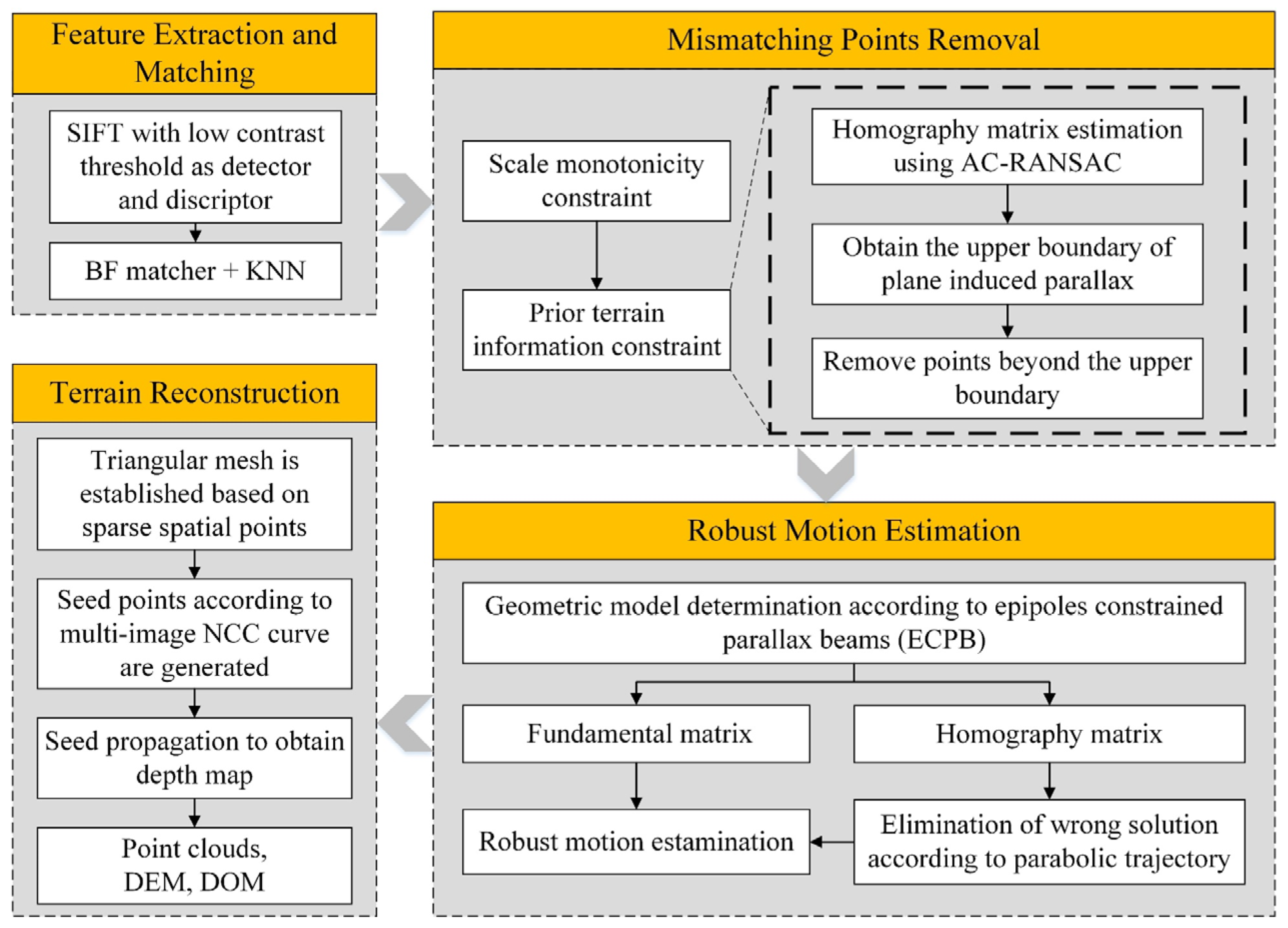
The four main steps of the TR-TR algorithm include feature extraction and matching, mismatching points removal, robust motion estimation, and terrain reconstruction. Details are as follows:
(I)
For the feature extraction and matching part, SIFT with a low contrast threshold is applied to extract and descript feature points, after which BF matcher with KNN (k = 2) is utilized to filter bad matches.
(II)
The TR-TR algorithm uses two constraints to remove mismatching points: the scale monotonicity constraint and the a priori terrain information constraint. The scale monotonicity constraint takes advantage of the fact that the feature point scale monotonically varies with the descent image order to remove mismatching points. The constraint of prior terrain information requires first finding the homography matrix (H) corresponding to the points in the scene plane by a contrario RANSAC (AC-RANSAC) method. Then, DEM of the landing area generated from the orbiter images is exploited as prior terrain information to find the upper boundary of the plane induced parallax (introduced in Section 2.2.2) corresponding to the homography matrix (H), and, finally, remove points beyond the boundary.
(III)
According to the two solutions obtained by the homography matrix (H) decomposition, two possible positions of epipoles are obtained as constraints to perform the epipoles constrained parallax beam (ECPB) algorithm. If the fundamental matrix is obtained, the determined motion solution can be obtained directly by decomposition of the fundamental. If the fundamental matrix cannot be obtained, the solution that does not conform to the parabolic descent trajectory constraint in the two solutions obtained by decomposition of the homography matrix (H) is eliminated to obtain the determined motion solution.
(IV)
After refining the motion by bundle adjustment, the accurate descent trajectory is obtained. A lot of sparse spatial points are also obtained when estimating motion between images in the previous step. Triangular mesh is established based on these sparse spatial points. Each triangle in the mesh is projected to all images that can see the triangle. Based on these projections, multi-image normalized cross-correlation score (NCC) curves are drawn and initial seed points are determined accordingly. Initial seed points are then propagated to obtain depth maps for generating dense point clouds. Finally, DEM and DOM of the landing area are generated based on dense point clouds.
The flow chart of the TR-TR algorithm proposed in this paper for processing the descent images is given below (Figure 2).

2.2.1. Feature Extraction and Matching

Compared with other operators, SIFT describes the position of points most accurately, which can improve the trajectory recovery accuracy. Therefore, SIFT is selected to extract and describe feature points in descent images. However, the uneven distribution of ground features in the landing area of Tianwen-1 leads to the emergence of large textureless areas in the descent images. Unfortunately, in these textureless areas, SIFT with default threshold in OpenCV (a famous open source computer vision library) is not able to extract sufficient feature points. In order to solve this problem, the contrast threshold of the SIFT operator should be set as small as possible.
The principle of feature point matching is to compare the Euclidean distance of two feature point descriptors as a similarity measure. For feature point p 1 in image I 1 , to find its matching point p 2 in image I 2 , the BF matcher combined with KNN ( k = 2 ) is used to return the two best matches p 21 and p 22 (with similarity measure s 1 and s 2 , respectively) from image I 2 . If s 1 / s 2 is smaller than a similarity ratio threshold (assuming s 1 < s 2 ), p 21 is considered to be the correct matching point. The BF matcher is better than the FLANN matcher because although the FLANN matcher is faster, the processing time of the descent images is sufficient. Since the landing camera moves forward along the descent trajectory, there will be overlapping areas in successive descent images. Hence, it is not enough to match feature points only in adjacent images, but it should be done in multiple consecutive images to obtain feature tracks.

2.2.2. Mismatching Points Elimination

Meng et al. uses RANSAC to search the fundamental matrix among all matching points, and removes the matching points that do not conform to the calculated fundamental matrix as mismatching points [24]. This method is suitable for a general scene, but not suitable for the scene in the Tianwen-1 descent images. The scene in the Tianwen-1 descent images is a planet surface with flat terrain, resulting in (quasi-) degenerated data. (Quasi-) degenerated data may not provide sufficient constraints on the fundamental matrix due to rank deficiency; hence, an incorrect fundamental matrix may be obtained. RANSAC consistent with an incorrect fundamental matrix will remove a large number of correct matching points. Besides, Meng’s method does not take advantage of the characteristics of the descent images, such as the monotonicity of scale changes. Based on this problem, the TR-TR algorithm chooses to use the homography matrix to eliminate mismatching points instead of using the fundamental matrix. Since most of the points (or all points) in the (quasi-) degenerated data are located in a scene plane, these data may not form sufficient constraints on the fundamental matrix, but it must form sufficient constraints on the homography matrix. Therefore, a robust homography matrix can be obtained. In addition to robustness, the homography matrix has another advantage that it can make use of the prior terrain information, which the fundamental matrix cannot do. Apart from the consistency method, the TR-TR algorithm also makes use of the scale monotonicity of the descent images.
In the TR-TR algorithm, the scale monotonicity constraint is utilized first to eliminate part of the mismatching points. The landing camera’s forward motion causes the scale (obtained from the SIFT descriptor) of one feature track in the descent images to increase monotonically with the acquisition time. As a result, feature tracks not meeting this condition must contain mismatching points. For such feature tracks, the contained features whose scale do not vary monotonically are removed to maintain the scale monotonicity of the feature tracks.
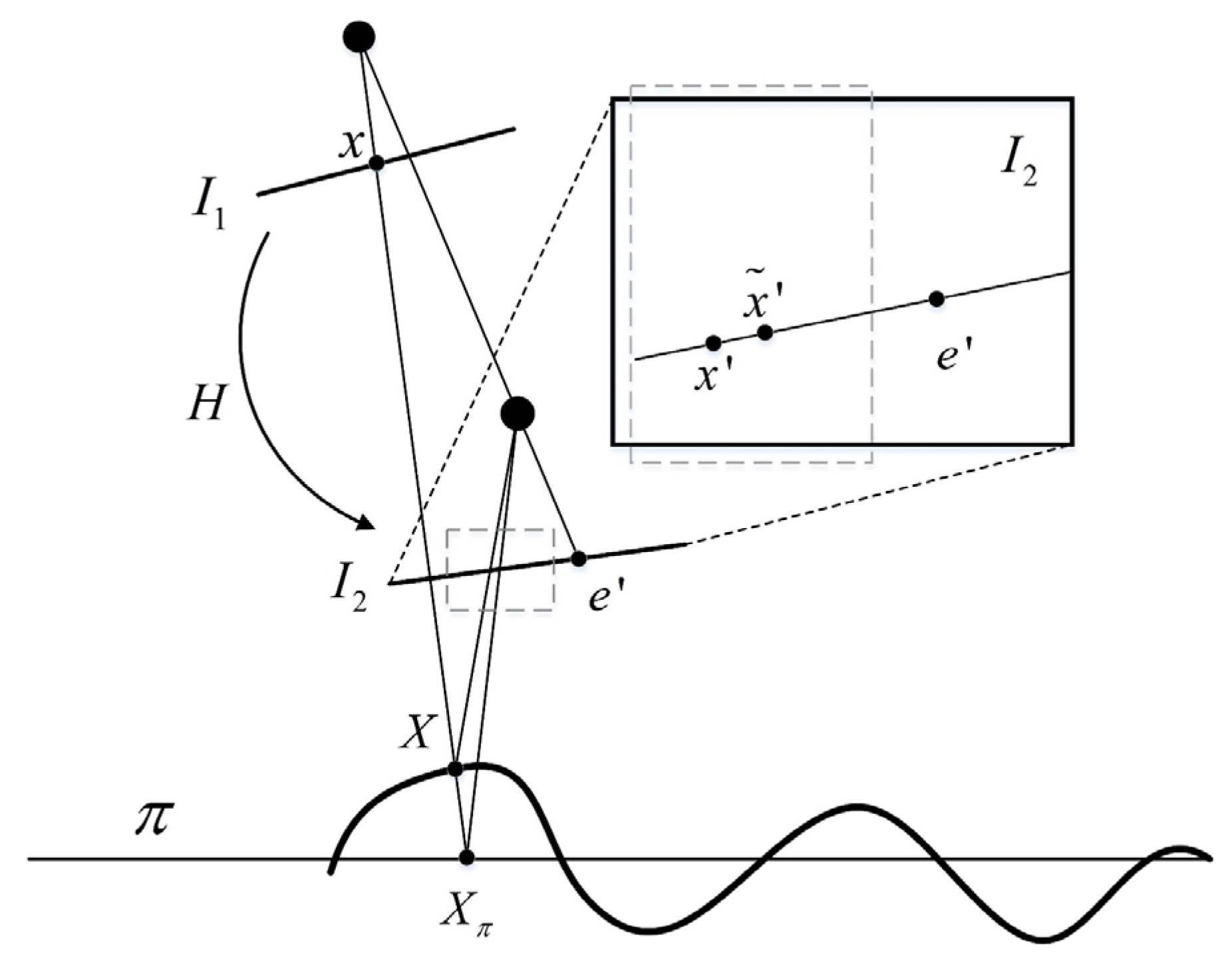
Next, mismatching points are eliminated by prior terrain information constraint. Data are degenerate when all points lie inside a plane, whereas those data are quasi-degenerate when most points lie inside a plane with the rest lying outside the plane. The terrain in the landing area of Tianwen-1 is flat and approximates a scene plane for the landing camera. Most of the ground points are inside the scene plane, with occasional undulating ground points (e.g., volcanoes, gullies, impact craters) located outside the scene plane. The maximum elevation difference of the landing area can be evaluated from the DEM generated by the orbiter images of Tianwen-1. Restricted by the maximum elevation difference, when the approximate acquisition height corresponding to each descent image is known (supplied by laser altimeter), the plane induced parallax (introduced in Figure 3 and denoted as ρ ) of points outside the plane must have an upper boundary (denoted as ρ m a x ). The points beyond the boundary must be mismatching points to remove.
In order to obtain the plane induced parallax of corresponding points, the homography matrix needs to be solved first. The homography matrix computed in conjunction with the AC-RANSAC framework is robust to noise and mismatches [44]. The number of false alarms ( N F A ) is determined by AC-RANSAC as:
N F A ( H , k ) = ( n 4 ) ( n k ) ( k 4 ) ( ε k 2 α 0 ) k 4
where H is the homography matrix to be tested, ε k denotes the k th minimum residual, α 0 indicates the proportion of the area of the circle with a radius of one pixel in the image, n represents the number of total matching points.
The homography matrix ( H ) is considered valid if
N F A ( H ) = m i n 5 k n N F A ( H , k ) 1
Let H ^ indicate the homography matrix obtained by AC-RANSAC and ε the corresponding maximum residuals; the correct matching points set P can then be figured out according to H ^ and ε . Introducing set U as the total matching points, the rest of the matching point set is obtained as the complementary set of P from U , which is represented by U P . U P = implies that all matching points lie inside the plane corresponding to H ^ , which means that the data are degenerate. If not, matching points with too large plane induced parallaxes are considered to be mismatching points and are removed from U P , leaving the matching points set U P ρ < ρ m a x .

2.2.3. Robust Motion Estimation

Meng et al. uses RANSAC to search the fundamental matrix among all matching points, and decompose the fundamental matrix to obtain the motion [24]. In this way, there is an obvious disadvantage that the (quasi-) degenerated data caused by flat terrain will easily result in an incorrect fundamental matrix, and then get the wrong motion. By contrast, in the TR-TR algorithm, motion can be obtained robustly. As mentioned in the previous section, a robust homography matrix is obtained from (quasi-) degenerated data. Based on the obtained homography matrix, the corresponding fundamental matrix is estimated according to the relationship between the fundamental matrix and the homography matrix if the data provide sufficient constraints. Specifically, the robust fundamental matrix is estimated from the points (may including some mismatching points) located outside the plane corresponding to the obtained homography matrix using the epipoles constrained parallax beam method [38]. The robust motion is obtained by decomposing the fundamental matrix. If the data cannot provide sufficient constraints, the fundamental matrix will not be obtained. For such cases, the homography matrix is decomposed into two motion solutions. The TR-TR algorithm utilizes the parabolic property of the descent trajectory to eliminate the one that does not match the actual situation, and the remaining motion solution is robust.
Continuing from the previous section, U P ρ < ρ m a x = means that matching points, except those in the plane corresponding to H ^ , are all mismatching points, indicating a case of degenerate data. Conversely, if U P ρ < ρ m a x , there may exist correct matching points that lie outside the plane which provides constraints on the epipolar geometry to estimate the fundamental matrix.
H ^ is decomposed to obtain two possible epipoles e 1 and e 2 on the second image. The i th matching point is imaged at x i and x i for the first and second view, respectively. Ideally, the line between x i and H ^ x i would either pass through point e 1 or e 2 , corresponding to the two possible fundamental matrices F 1 ^ or F 2 ^ , respectively. However, in practice, it will not happen because both x i and H ^ x i are corrupted with noise. For simplicity, let x i and H ^ x i have the same point error that has a distribution area of the circle of radius ε with the point as the center since ε (figured out from AC-RANSAC) represents point error more accurately. The parallax beams [38] of x i and H ^ x i are drawn to judge if they cover e 1 or e 2 . Set the initial values of two counters N F 1 ^ and N F 2 ^ to be zero. Let N F 1 ^ = N F 1 ^ + 1 if e 1 is covered. Similarly, let N F 2 ^ = N F 2 ^ + 1 if e 2 is covered. The geometric model ( M ) of the image pair is determined as:
{ M = H ^ ,   i f   N F 1 ^ = N F 2 ^   M = F 1 ^ ,   i f   N F 1 ^ > N F 2 ^   M = F 2 ^ ,   i f   N F 1 ^ < N F 2 ^
A definite solution of motion comes from the decomposition of the fundamental matrix if M = F 1 ^ or M = F 2 ^ when knowing the camera matrix (K), whereas two possible solutions come from the decomposition of the homography matrix if M = H ^ . In fact, the parabolic property of the descent trajectory can be used to remove the unrealistic solution.
For convenience, x and y are defined [45]:
x = R T t | | t | |
y = | | t | | n
where R and t are the rotation matrix and translation vector normalized with respect to the depth of the plane of which the normal vector is represented by n .
Equations (5) and (6) show the relationship of two solutions obtained from the decomposition of the homography matrix, which is distinguished by subscripts a and b:
y b = ± | | y a | | ρ ( y a + 2 x a )
x b = 1 ρ ( ν | | y a | | y a | | y a | | x a )
where,
ρ = | | x e × y e | | 2 + ( x e T y e + 2 ) 2
ν = 2 ( x e T y e + 1 )
where,
e = { a , b }
Replacing (3) and (4) into (5) and (6), we can figure out that
n b = ± | | t a | | | | n a | | ρ | | t b | | ( | | t a | | n a + 2 R a T t a | | t a | | )
R b T t b = | | t b | | ρ ( ν n a | | n a | | | | n a | | R a T t a )
For one descent image pair of Tianwen-1, denoting O L as the camera center of the image taken at a lower altitude and O H as the camera center of the image taken at a higher altitude, there are two possible locations of O H (marked as O H a and O H b ) corresponding to two solutions if the camera O L is fixed with a view along the inverse direction of the y-axis of the camera coordinate system, as shown in Figure 4. It can be concluded from Figure 4 that the angle θ a between | | t a | | n a and O L O H a satisfy Equation (12) when assuming that O H a is in the quadrant { + x , z } ( O H a must be located in the quadrant { ± x , z } , since O H a is higher than O L ):
π / 2 < θ a < π
R a T t a (equaling the vector O H a O L ) has the same direction as 2 R a T t a | | t a | | , which implies that 2 R a T t a | | t a | | is a vector pointing to the quadrant { x , + z } . Equation (8) shows there are two possible solutions (in opposite directions of { x , + z } and { + x , z } according to the vector algorithm) of n b , among which apparently only the one solution pointing { x , + z } fits the reality.
ν n a | | n a | | ( ν > 0 ) has the same direction with | | t a | | n a , which points towards the plane perpendicularly. At the same time, | | n a | | R a T t a has the same direction with 2 R a T t a | | t a | | . It can be inferred from Equation (9) that R b T t b points to the quadrant { + x , ± z } since ρ > 1 . Obviously, O H b O L cannot point toward { + x , z } because O H b is higher than O L , which indicates that R b T t b actually points to the quadrant { + x , + z } , since R b T t b = O H b O L . Therefore, the angle θ b between R b T t b and n b satisfies the following equation:
0 < θ b < π
where 0 < θ b < π / 2 violates the visibility constraint of I H , so:
π / 2 < θ b < π
In Figure 4, two surfaces are drawn for Solution a and Solution b separately, which does not correspond to the actual situation in which there is only one surface that can be used to analyze the relationship between two possible locations of O H when fixing O L . Next, the surfaces of Solution a and Solution b are brought together to get the following schematic diagram:
According to Equations (12) and (14), as shown in Figure 5, it can be concluded that O H a and O H b must not lie on the same side of the surface normal line of the Mars surface at the point O L .
The above discussion is for the case when O H a lies in the { + x , z } quadrant. It still satisfies the above conclusion when O H a lies in the { x , z } quadrant due to the property of equivalent exchange of the two solutions [45].
For simplicity, a 2D case has been given above. It is not difficult to deduce that two solutions follow the same principle in the actual 3D case, except that the normal line is replaced by the normal plane which is perpendicular to the horizontal component of the velocity of the lander and passes through O L . In practice, the solution in which O H lies on the opposite side of the direction of the horizontal component of the normal plane’s velocity is the correct solution.

2.2.4. Terrain Reconstruction

Due to the forward motion of the descent images, the epipole is located inside the image. The window correlation method used in binocular vision is not applicable in descent images. If we resample one image along the epipolar line to make their resolution equivalent as in stereo, then the images will be oversampled near the epipole while undersampled at the image boundaries. Hence, Meng proposed using the plane-sweep method to reconstruct the terrain [24]. The specific method is to use several parallel virtual planes to cut the terrain. For one point on image 1, the projection window of its correlating window on each virtual plane on image 2 can be obtained by homography projection. Consequently, several candidate windows are obtained on image 2 about the correlation window of that point on image 1. The ZNCC of the correlation window on image 1 and the candidate windows on image 2 are calculated as the correlation measure, and the depth value of the virtual plane corresponding to the candidate window with the greatest correlation is taken as the depth value of that point on image 1. The depth map of image 1 is generated by this method. Subsequently, Meng studied the shape of ZNCC curves and formulated rules to filter out ZNCC curves with poor conditions (such as too flat or with two similar peaks). A point whose ZNCC curve is qualified is selected as the initial seed point. Then, the initial seed points are propagated using BSFP strategy to generate a depth map [25].
Meng’s method has several disadvantages. Firstly, the method only discussed the depth recovery of two images, but did not utilize the other images. Secondly, the virtual planes used by this method in the plane-sweep algorithm has only one direction; thus, this method has low depth accuracy for the recovery of forward-tilting terrain, which is not good at the recovery of detailed terrain. Thirdly, this method does not use the sparse spatial points obtained in the previous motion estimation steps. These sparse spatial points are very accurate prior information which can be used to improve the terrain accuracy. In contrast, the TR-TR algorithm proposes the plane-sweep method using multiple images. The TR-TR algorithm uses virtual planes that do not have only one direction, so that they can better fit the small-scale undulating terrain of the Tianwen-1 landing area. TR-TR algorithm takes advantage of sparse spatial points to increase the accuracy of reconstructed terrain. Specific methods are as follows.
After camera motion refining and bundle adjustment, a series of sparse spatial points are obtained, which are employed to constitute a mesh containing many spatial triangles. The image I L with the lowest acquisition height is moved out from the image set obtained by searching images containing some triangle P , leaving an image set denoted as Γ = { I i | i = 1 N } . M virtual planes parallel to P are created around P and are marked as { V k   |   k = 1 M } . The homography H k i induced by V k between I L and I i in Γ is:
H k i = K ( R i R L 1 + R i ( C L C i ) n k T n k T X k ) K 1
where, K is the camera calibration matrix, X k represents a point passed through by V k , n k T is defined as the normal of V k , R i is the rotation matrix of I i , R L is the rotation matrix of I L , C i is the location of I i and C L is the location of I L .
Marking P L and P i as projections of P on I L and I i ( I i Γ ) , respectively, the NCC of pixel ( u , v ) P L between I L and I i ( I i Γ ) is given:
C k i ( u , v ) = ( u , v ) W c w ( u , v ) · τ ( I L i k ( u , v ) , I i ( u , v ) )
where W c is the correlation window, w ( u , v ) indicates the weight of pixel ( u , v ) and τ ( I L i k ( u , v ) ,   I i ( u , v ) ) computes the dissimilarity of I L i k and I i with regard to ( u , v ) . w ( u , v ) is obtained by:
w ( u , v ) = { 1 , ( u , v ) P i e d , ( u , v ) P i
where d is the distance between ( u , v ) and P i , implying less weight corresponding to further distance.
τ ( I L i k ( u , v ) , I i ( u , v ) ) is defined as:
τ ( I L i k ( u , v ) , I i ( u , v ) ) = γ | | I L i k ( u , v ) I i ( u , v ) | | + ( 1 γ ) | | I L i k ( u , v ) I i ( u , v ) | |
where | | I L i k ( u , v ) I i ( u , v ) | | computes the L1-distance of I L i k ( u , v ) and I i ( u , v ) ’s grey value space, | | I L i k ( u , v ) I i ( u , v ) | | computes the absolute difference of the gray-value gradients of I L i k ( u , v ) and I i ( u , v ) , and γ is a user-defined parameter.
The final score C k ( u , v ) of ( u , v ) with respect to V k is obtained by summing up the C k i ( u , v ) calculated from all images in Γ :
τ C k ( u , v ) = i = 1 N C k i ( u , v )
The points at which the C k ( u , v ) curve fluctuated with respect to k fits the condition are selected as seed points, as well as sparse spatial points. The seed points are propagated within the triangle P L to generate the depth map of I L of triangle P , thus obtaining the point clouds of P . In the same way, the point clouds of other triangles are calculated and fused to obtain the final point clouds of the whole terrain. The terrain point clouds are projected to the horizontal plane in the vertical direction according to the Mars geographic coordinate system to generate a dense Delaunay triangle network. For each triangle, the elevation and grayscale values of the raster points within the triangular surface slice can be obtained by interpolation based on the elevation and grayscale values of the three vertices. Using this method, the elevation and grayscale values of all raster points in the landing area can be obtained to generate the DEM and DOM of the landing area.

3. Field Experiment

3.1. Experiment Overview

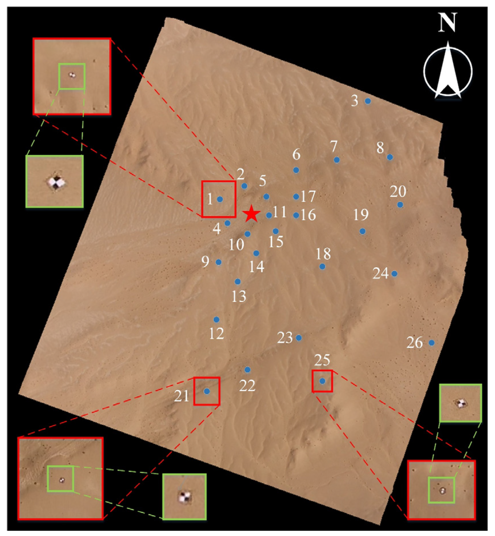
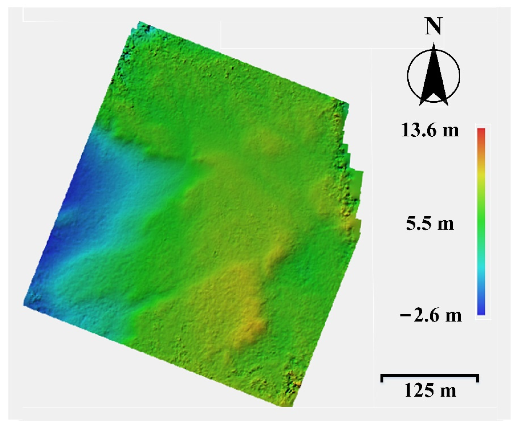
In order to verify the method proposed in this paper, a corresponding field experiment in the Red Cliff area with a Mars-like terrain was designed. The experimental data were captured in November 2019 by the unmanned aerial vehicles (UAVs), DJI Phantom 3 and Phantom 4, during descent when simulating the lander of Tianwen-1, through which far more than 2000 images were acquired. The Red Cliff area is located in the Dachaidan region of Qinghai Province, China. It is the first Mars simulation basement in China and has topographic of great value for studying planetary landforms [46]. Before aerial photography, a number of checkerboard grid plastic boards were deployed as ground control points (Figure 6). The coordinates of the ground control points were measured using the Topcon total station. The true value of the position and pose of the camera corresponding to each descent image were evaluated from the coordinates of the ground control points. In addition to the simulated landing, the UAV flew along multiple airstrips and acquired a large amount of image data which were processed to obtain the true values of the DEM of the experimental area (Figure 7). It can be seen that there are three similarities between the landforms of the experimental area and the landing area of Tianwen-1 (refer to the Tianwen-1′s orbiter image): (1) the terrain is relatively flat (Utopia Plain of Mars); (2) both contain striated feature (sand ridges on Mars); and (3) both contain small areas of obvious topographic relief (impact craters on Mars).

3.2. Matching Accuracy and Initial Motion

The combination of the mismatching points elimination methods proposed in this paper achieves higher matching accuracy. In addition, the proposed initial motion estimation algorithm in this paper achieves more robust and accurate motion results. In order to verify this, the result of Meng’s method [24] (searching fundamental matrix directly by RANSAC) is compared in the experiment (Figure 8). The comparison of matching accuracy and the comparison of initial motion error are put together in this section because the matching result directly affects the accuracy and robustness of initial motion estimation.

3.2.1. Matching Accuracy

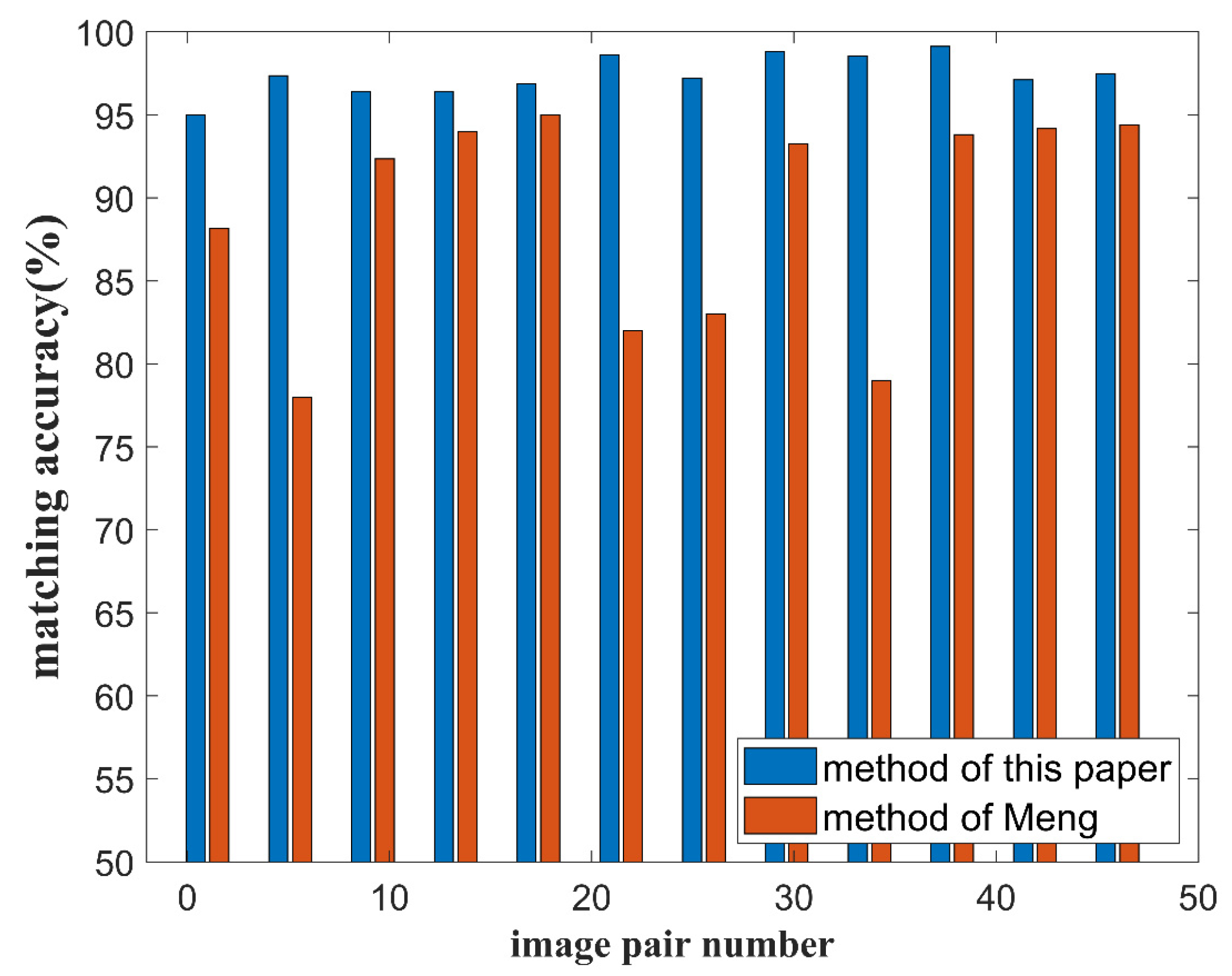
A combination of scale constraints and homography matrix constraints are proposed to eliminate mismatching points in this paper. In the experiment, the true values of the corresponding fundamental matrices can be evaluated based on the true values of the translations and poses of the descent images. It is assumed that the fundamental matrix of an image pair { I 1 , I 2 } is denoted as F . A matching point is marked as x on image I 1 and x on image I 2 . The epipolar line through x is represented by l . Taking the distance from x to l as a measure, a matching point with such distance less than one pixel is considered to be a correct matching point. The matching accuracy is obtained by dividing the number of correct matching points by the total number of matching points. Twelve out of a total of forty-five pairs were sampled to compare matching accuracy. It is obvious that the matching accuracy of four image pairs obtained by Meng’s method is too low. This is due to the elimination of correct matching points since the incorrect fundamental matrices are evaluated from (quasi-)degenerate data. These phenomena appear randomly among image pairs, whereas the geometric models obtained by the method of this paper avoid this randomness and thus can robustly eliminate the mismatching points. Apart from this, the matching accuracy of the Meng’s method is still not as high as that obtained by the method of this paper. The reason for this is that Meng’s method does not consider using the scale constraint of descent images to eliminate the mismatching points.

3.2.2. Initial Motion

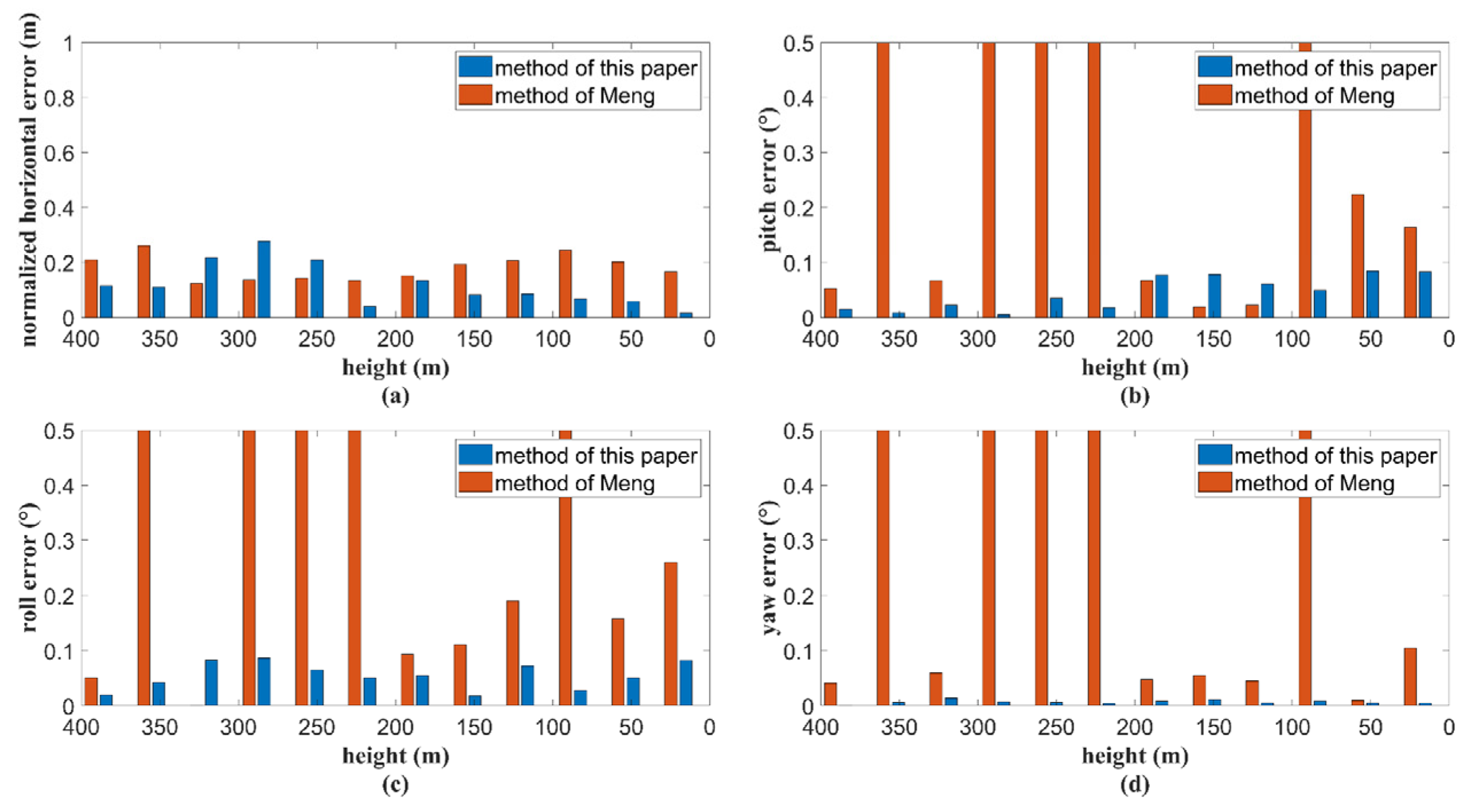
The ECPB algorithm was used to estimate an accurate geometry model of an image pair, followed by the utilization of parabolic trajectory to remove the ambiguity of solutions derived from the decomposition of the homography matrix. In order to verify that the proposed algorithm can obtain more robust motion results, the relative pose and translation of twelve image pairs selected from total forty-five image pairs by equal interval are compared in the experiment with Meng’s method [24]. Compared to the vertical translation, the horizontal translation has more influence on the accuracy of terrain reconstruction. Thus, only the horizontal translation error (obtained by differentiation from the true value) is compared. The rotational angle error calculated by Meng’s method is sometimes too large (gross error). In order to reflect the details of the comparison, the maximum value of the angle error is set to 0.5°, for which reason all angle errors over 0.5° are displayed as 0.5° (Figure 9).
From Figure 9, it can be seen that almost half of the motion solutions obtained through Meng’s method [24] have gross errors in angle, which means they are completely wrong solutions although they do not have gross errors in horizontal motion error. These wrong motion solutions are considered to be results of decomposition of incorrect fundamental matrices obtained from the (quasi-)degenerate data. In fact, this result corresponds to the matching accuracy result in Figure 9 (the incorrect fundamental matrices lead to very low matching accuracy and wrong pose solutions).The results of this paper’s algorithm do not have gross errors, which provides stable initial values for the subsequent steps of bundle adjustment.
It can also be seen from Figure 9 that the accuracy of other correct pose solutions obtained by Meng’s method is still not as high as that obtained by this paper’s method, which is mainly because this paper’s method has higher matching accuracy in other image pairs than the method of Meng.

3.3. Feature Points Extraction and Refined Motion

The feature points extraction method proposed in this paper obtains denser and more uniform feature points, which achieves more accurate refined motion results after bundle adjustment. In order to verify it, the feature points extracted by SIFT with default threshold in OpenCV is compared in the experiment.

3.3.1. Feature Points Extraction

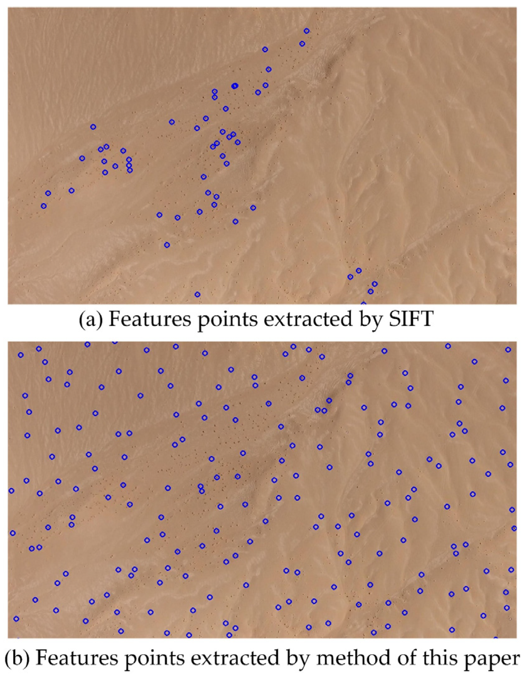
In OpenCV, the default contrast threshold for SIFT is 0.04. In the method of this paper, this value is set to 0.01; thus, more matching points in the textureless area of the descent images can be obtained; but at the same time, there will be more points in other texture-rich areas, resulting in an increase in computation. Hence, the method of this paper also sets the maximum number of extracted feature points by region to limit the number of feature points that are too dense in some areas of descent images.
In order to visually compare the extraction of feature points, a descent image containing a textureless area is selected to show the results of the two algorithms (Figure 10).
It is shown in Figure 10 that evenly distributed feature points are obtained by the method of this paper. These feature points are matched across all descent images according to the method described in Section 2.2.1 to obtain a large number of feature tracks. The comparison of the number of feature tracks obtained by the SIFT and the method of this paper is displayed in Table 3. Feature tracks of different lengths (number of images spanned by a feature track) are shown in the table.

3.3.2. Refined Motion

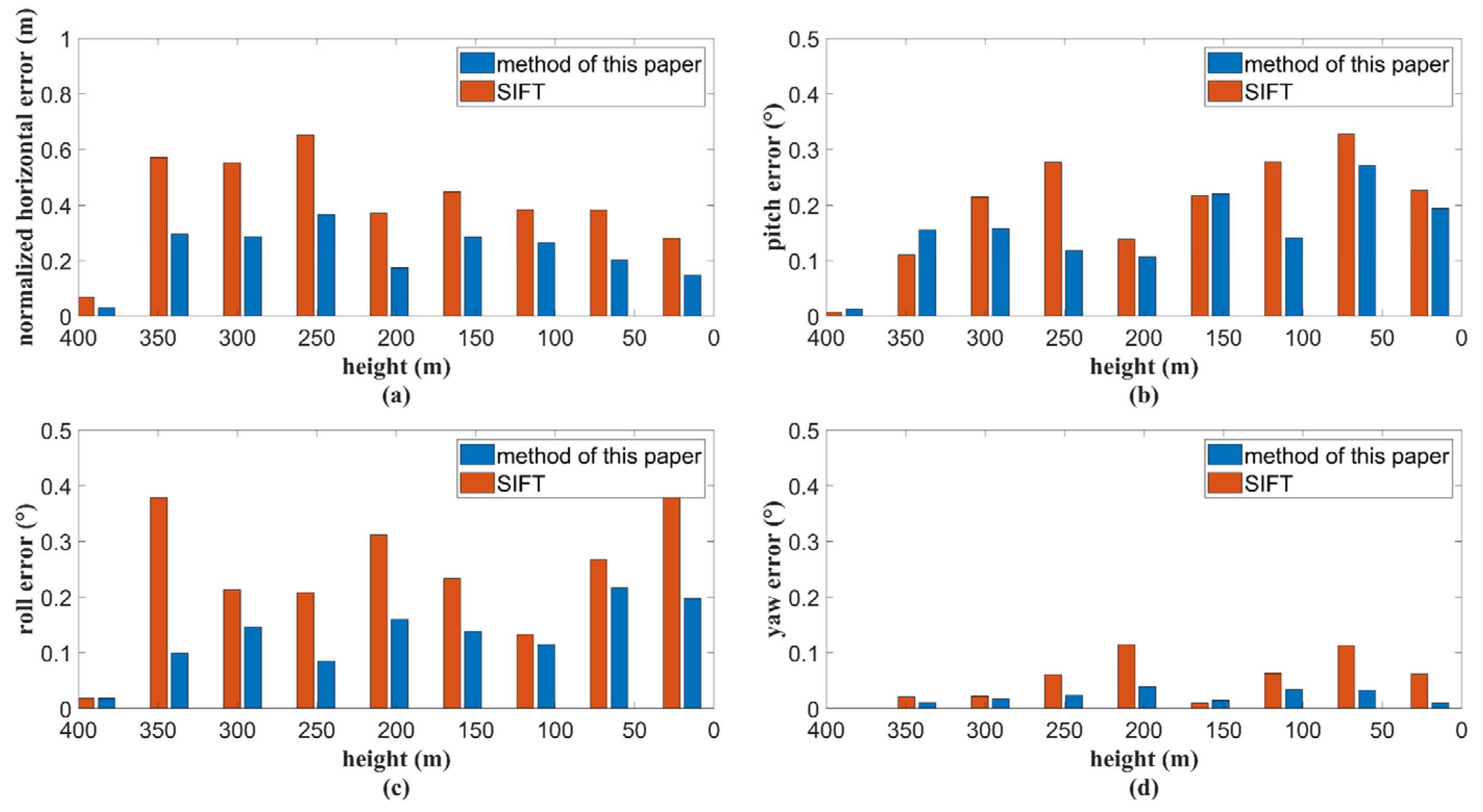
Employing reliable initial values, the uniform and dense feature points extracted by this paper’s algorithm and the SIFT feature points extracted by OpenCV with default threshold are used as the observed data of the bundle adjustment. After making a difference with true value, camera pose and translation errors are displayed for comparison (Figure 11).
It can be seen that uniformly and densely extracted and matched feature points help to obtain a more accurate motion. This is the result of control points involved adjustment. The error is small at the beginning of the descent, followed by a slow accumulation with descending height. The calculation results using feature points extracted by OpenCV fluctuate more, and the results of this paper have higher stability.

3.4. Terrain Reconstruction

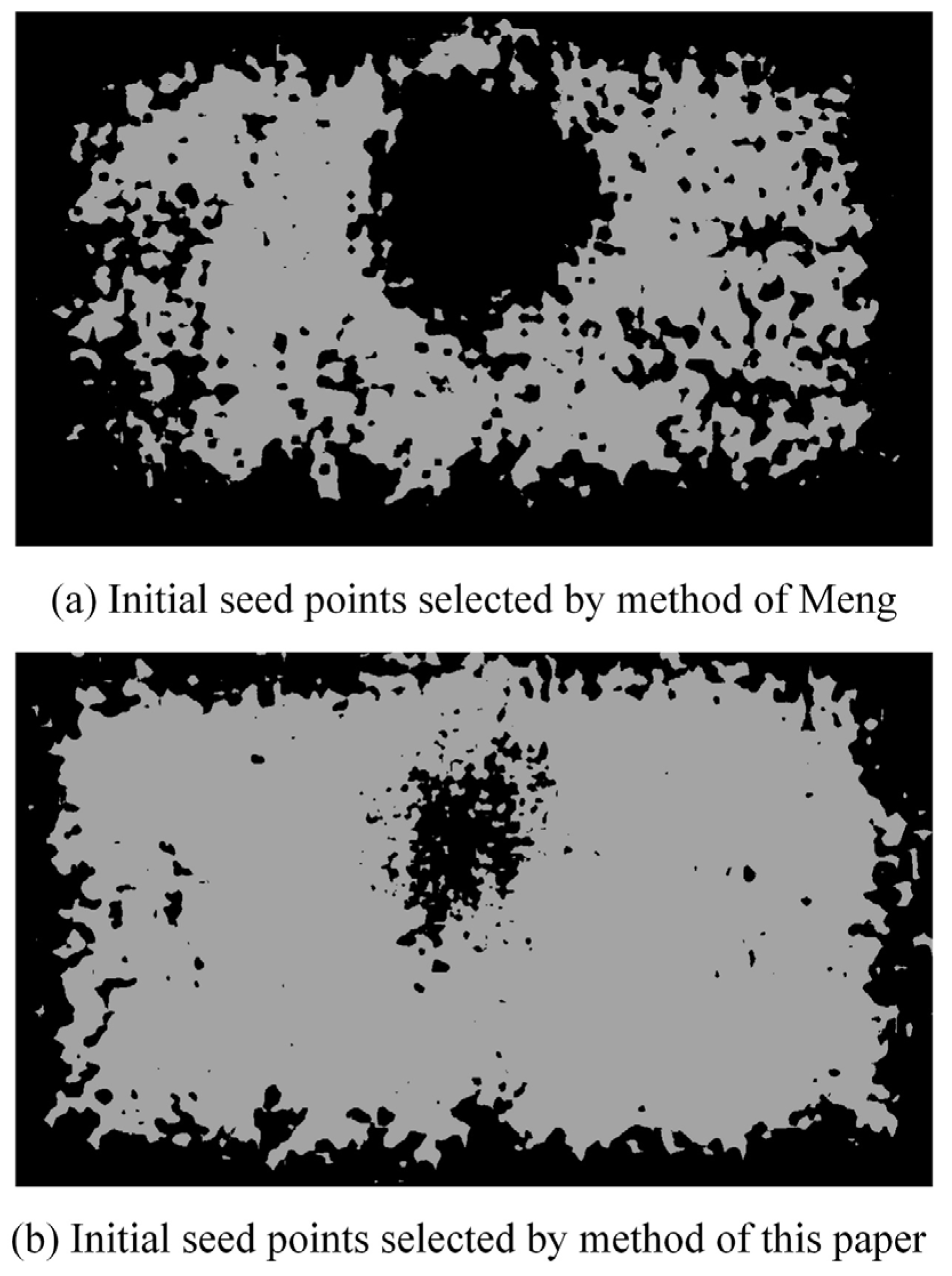
Regarding terrain reconstruction, the method of this paper adopts the plane sweep algorithm with multiple images in triangular units, whereas the previous method is the plane sweep algorithm with just image pairs in image units. In order to compare the number of initial seed points, a descent image is selected in the experiment, with all the initial seed points obtained by the method of this paper in the area covered by this image projected onto it for comparison with the initial seed points of this image calculated by Meng’s method (Figure 12) [24,25].
Clearly, in Figure 12, there are missing initial seed points in the circular area around the center of the image. This region, in which the variations in parallaxes are not sensitive to changes in virtual plane depth, is actually the region near the epipole of the image, resulting in a score curve that is too flat for pixels to meet the seed point selection condition. Overall, it seems that the proposed method in this paper yields a much larger number of seed points, even in the region near the epipoles.
In order to compare the terrain reconstruction error, the true terrain point clouds are projected to a selected descent image to obtain the ground-truth (GT) depth map. The depth maps of two methods are generated by projecting point clouds reconstructed by the methods of this paper and Meng’s to the selected descent image. Then, the depth error maps of two methods are evaluated through making difference with the GT depth map respectively. (Figure 13).
As shown in Figure 13, the depth error maps obtained by two methods both show a contour-like distribution due to the plane sweep algorithm, in which the error variation estimated by the method in this paper is smoother. In the area near the epipole, the error obtained by Meng’s method reaches more than 0.40 m, whereas the error evaluated by the method in this paper does not exceed 0.25 m. Apart from the area near the epipole, the method in this paper also calculates a lower error, which indicates that the accuracy of terrain reconstruction has been significantly improved in this paper.
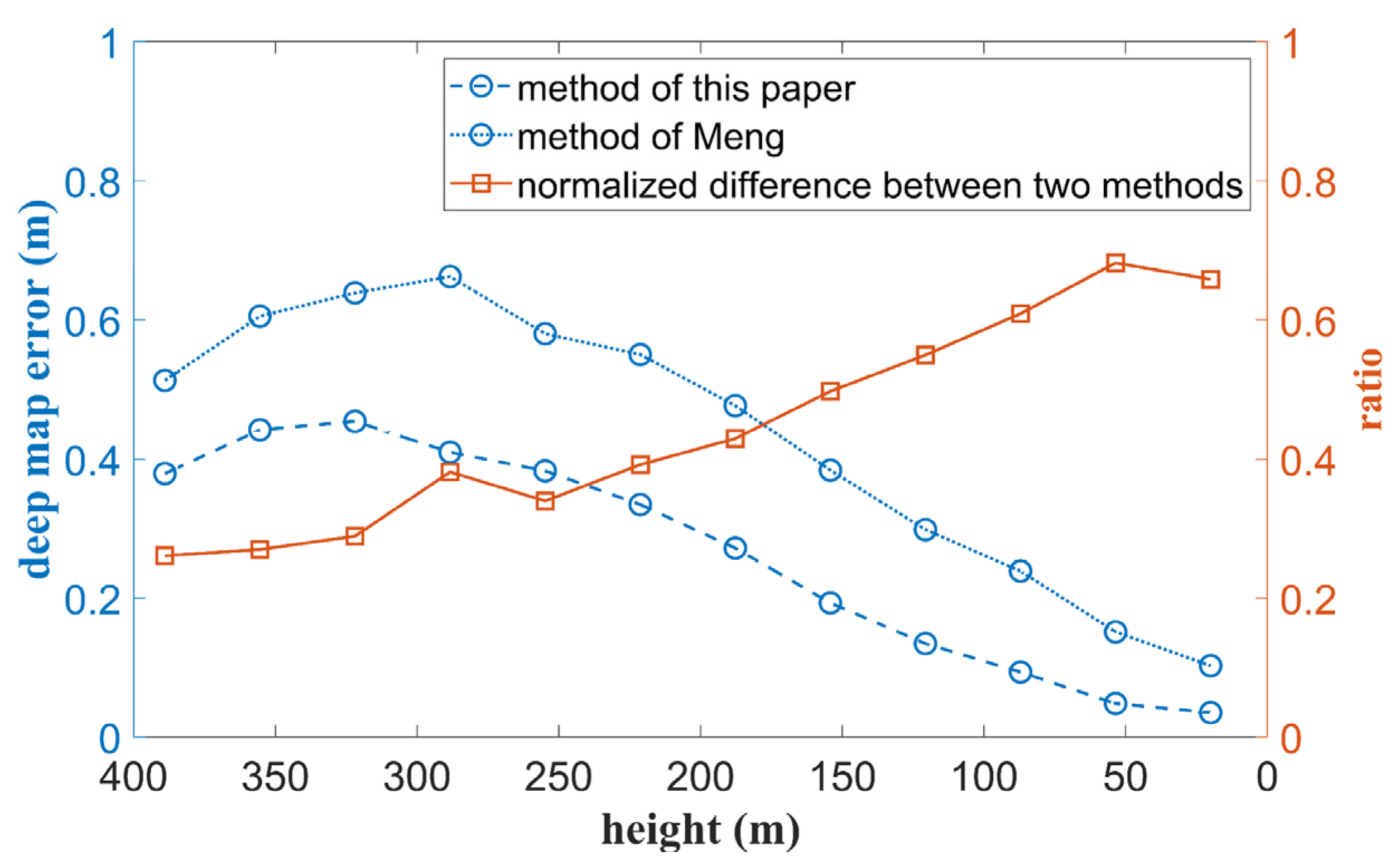
The average value of depth error maps of twelve images selected by equal interval are obtained for comparison between the methods of this paper and Meng’s (Figure 14) [24,25].
It can be seen from Figure 14 that the error of the depth map obtained by both methods has a tendency of first increasing and then decreasing with the landing process. The reason for the increase is probably the gradual decrease in the tilt angle of the photographic baseline, resulting in a small swing of the ray that creates a large variation in the vertical direction, whereas the later decrease is caused by the increasing ground resolution of the image when approaching the surface. During the whole landing process, it is illustrated that the advantage of the method proposed in this paper increases with a lower acquisition height of images. This is because at a low acquisition height, the method of this paper exploits multiple images to score the correlation instead of just two images used by Meng’s method. The other images acquired from higher altitude have larger tilt angles which alleviate the insensitivity of depth changes to parallax variation.

4. In-Orbit Data Processing

In the Tianwen-1 mission, using the TR-TR algorithm proposed in this paper, the corresponding positions and poses of the Tianwen-1′s landing camera during the EDL were recovered by processing the descent images, based on which the descent velocity was analyzed. Finally, the DEM and DOM of the landing area of Tianwen-1 were generated.

4.1. Footprint Map

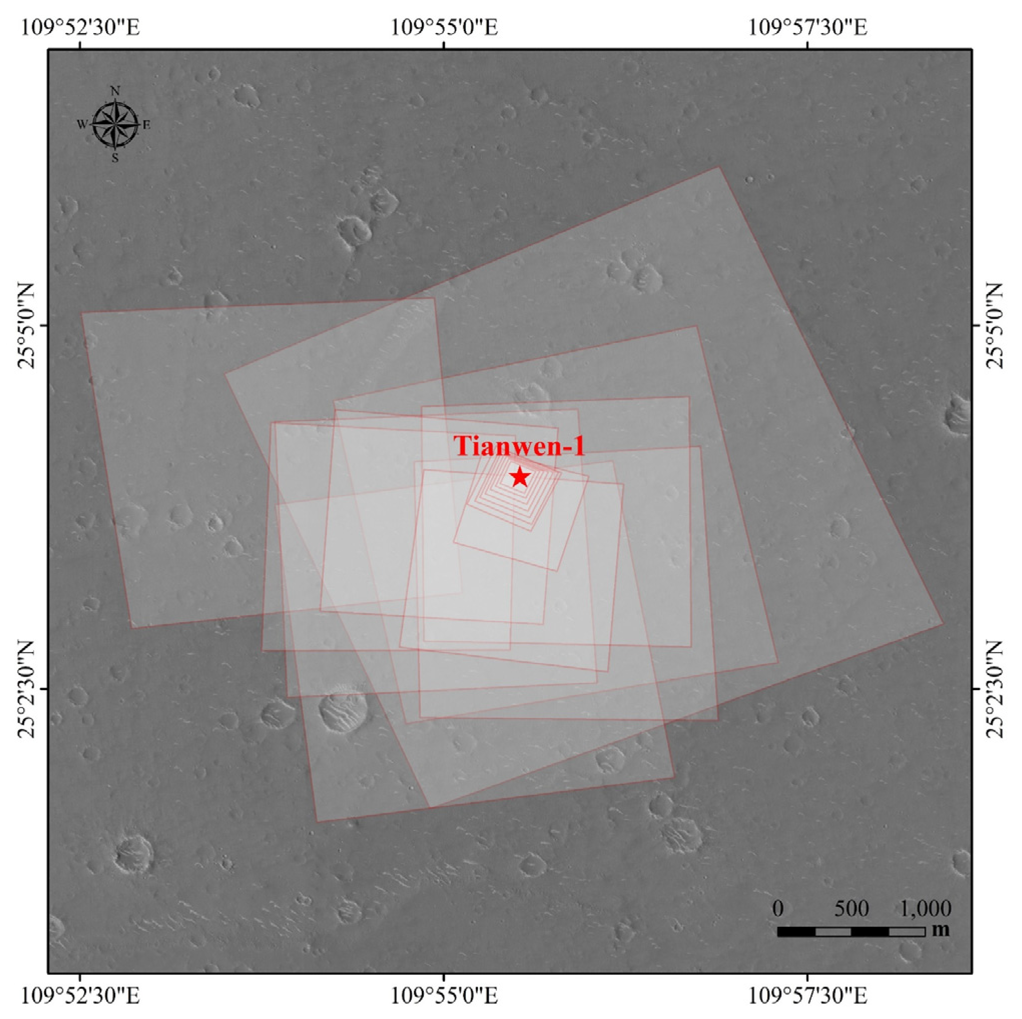
Based on the descent images of Tianwen-1, a footprint map was created. The footprint map shows the projection field of each descent image (the broader the field, the higher the acquisition height), which is more intuitive for us to understand the sampling method of the descent images. It is evident from Figure 15 that in the first half of the descent, there was a large swing of the landing camera which swung in the changing direction of mainly east–west and slightly north–south. A more violent swing of the landing camera denotes more deformation of the image and a greater distance from the landing site to the intersection of the camera’s optical axis with the surface of Mars. Besides, it also leads to a larger area far from the landing site covered by an image and a smaller overlap area with other images. In the second half of the descent, the pose of the landing camera gradually stabilized with a smaller swing in a mainly east–west and slightly north–south direction, along with the gradual disappearance of the deformation of the image. As the center of the image gradually approached the landing site, the overlapping area of adjacent images gradually becomes larger, with the north direction of the camera gradually shifting from the northwest to northeast, indicating that a clockwise rotation in the horizontal plane has occurred in the lander. It was found that descent images cover mainly a large area to the east, west, and south of the landing site, as well as a small area to the north of the landing site. The last few images taken before landing demonstrated that the camera was no longer swinging and no longer rotating horizontally during the final stage of descent. The upper borders of the descent images were more densely distributed, whereas the lower borders were more sparsely distributed, indicating that the horizontal moving component was directed from southwest to northeast at the final stage of descent.
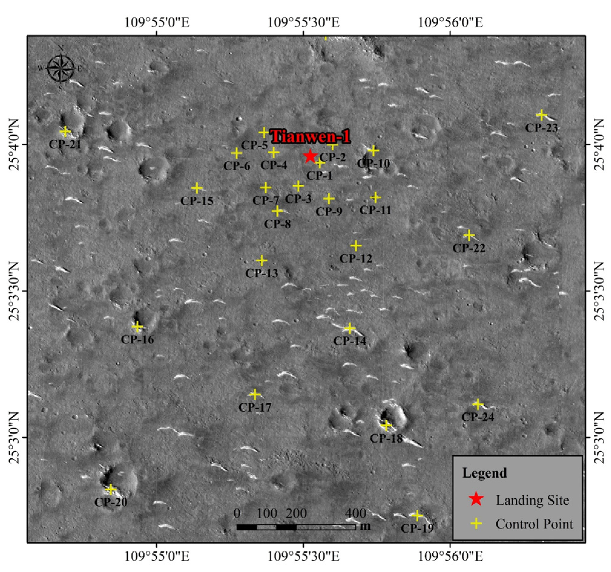
The descent trajectory and landing area terrain reconstructed from the descent images of Tianwen-1 are in the camera coordinate system corresponding to the first descent image, in which case the space relationships between the cameras are based on a hypothetical scale. Therefore, the result needs to be registered under the Mars geographic coordinate system, for which purpose a total of 24 ground control points were selected, as shown in Figure 16.
Figure 16 shows that the distribution range of ground control points gradually tightens from the southern region of the landing site toward the north, because the coverage of the descent image gradually shrinks with the landing process from a large area south of the landing site to the small area around the landing site. Most of the ground control points are mainly located in the southern region of the landing site, with few in the northern region, leading to an asymmetrical distribution from north to south but a basically symmetrical distribution in the east–west direction. The reason for this is the smaller imaging range of the landing camera covering the northern region of the landing site (refer to the footprint in Figure 15). In addition, the topographic information of the landing area can be obtained in advance based on the DEM generated from the images acquired by the Tianwen-1′s orbiter. Compared with the rugged topography of the northern region of the landing site, the southern region is flatter, which can reduce the risk of obstacle interference when the Zhurong rover carries out inspection and exploration work. Hence, the accurate acquisition of topographic information in the southern region of the landing site is more conducive to decision-making departments on the Earth to provide data support for the subsequent Zhurong rover’s path planning, which is also an important reason why the ground control points are mainly located in the southern region of the landing site.

4.2. Recovery of Trajectory and Velocity

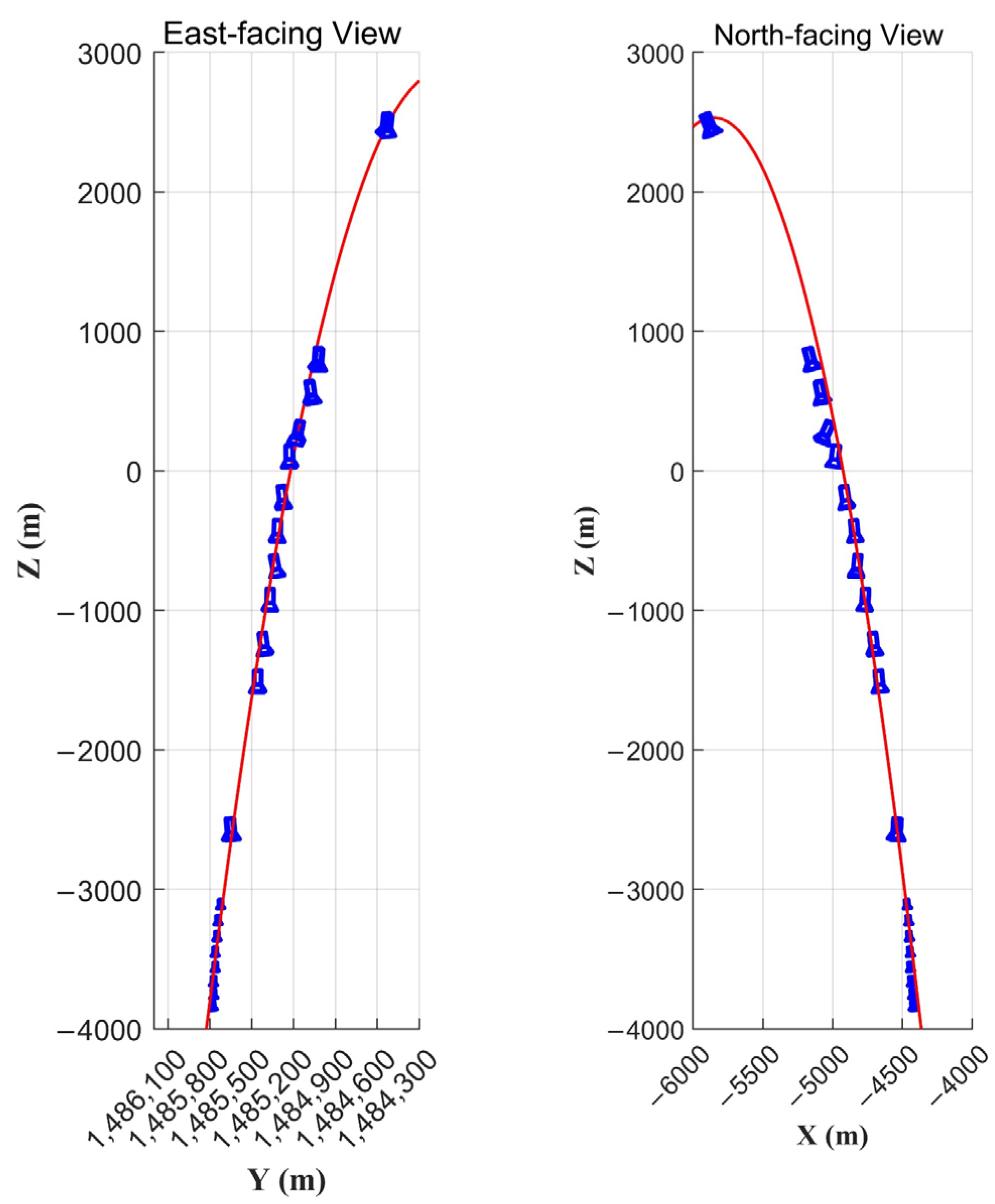
The positions and poses of the recovered landing camera during the EDL in the Mars geographic coordinate system are shown in Figure 17.
In Figure 17, the landing camera is represented by a polyhedron, so that not only the descent trajectory of the landing camera can be seen, but also the camera poses corresponding to each descent image. In order to facilitate the display, the simplified models of the landing camera corresponding to the lowest eight descent images are reduced to a certain size. This is due to the fact that the interval heights of those eight images became significantly smaller because of decreasing landing velocity. As indicated in Figure 17, there are three adjacent descent image positions with large intervals, namely, View1 (V1, and the same next) and V2, V11 and V12, and V12 and V13. The reason is that the sampling intervals of the descent images at the other positions are 4.096 s, whereas the sampling intervals of the camera became longer when these few images were taken; the sampling interval is 28.672 s between V1 and V2, 15.737 s between V11 and V12, and 12.936 s between V12 and V13 (refer to Section 2.1). Therefore, this phenomenon does not illustrate that the descent velocity has changed dramatically at the positions corresponding to these few images. The analysis about the footprint can be verified by Figure 17, the lander swings more in the east–west direction and less in the north–south direction during the EDL. The swing becomes negligible during the descent process corresponding to the last eight images, especially the swing in the east–west direction. During the time frame of the 20 descent images in total, the lander descended over 5000 m, spanning a distance of about 800 m from south to north and about 1100 m from west to east, for a total of about 1360 m in the horizontal direction, with the horizontal movement component pointing from eastward to northeastward.
The quadratic curves in two directions are fitted respectively. In the east-facing View, the equation of the quadratic curve is (4-bit valid digits retained with integer bits less than 4):
z = 0.002350 y 2 + 7701 y 5,715,107,590
In the north-facing View, the equation of the quadratic curve is (4-bit valid digits retained with integer bits less than 4):
z = 0.002950 x 2 34.53 x 98,627
In order to verify that the descent trajectory has the property of parabola, the residual error in the XY-plane between the fitted curves and the actual trajectory value is obtained as in Table 4.
Statistically, the root mean square error (RMSE) and the coefficient of determination of the recovered trajectory are obtained, respectively (Table 5).
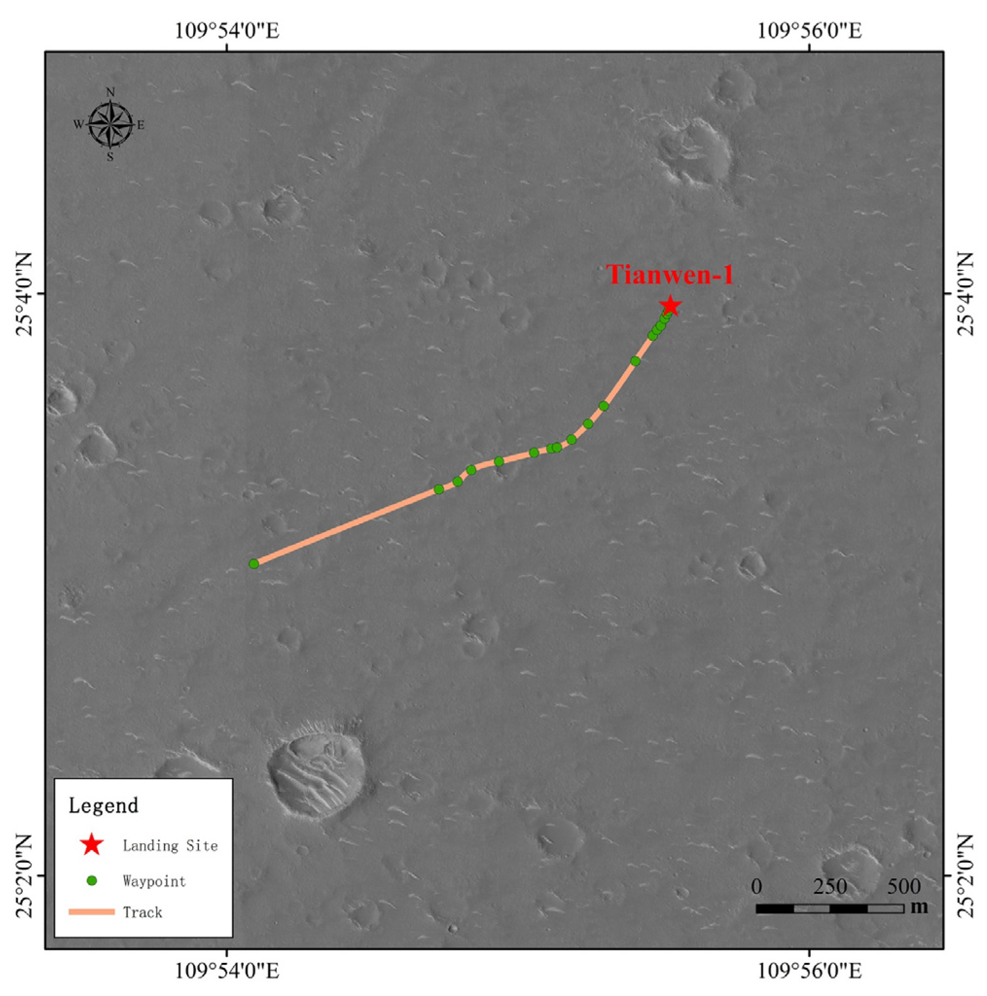
In the vertically downward direction, the descent trajectory can be seen as shown in Figure 18.
As illustrated by Figure 18, the overall landing trajectory is relatively smooth, except for slight fluctuations in the middle section. During the first half of the descent, the horizontal component of the velocity was mainly pointing from west to east, whereas in the second half of the descent, a slight left turn occurred, after which the direction of the horizontal component pointed from the southwest to northeast. The horizontal interval variation of the camera corresponds to the vertical interval variation of the camera in Figure 17. The V1 and the V12 far away from adjacent images, which is also the same situation in Figure 17. In the final stage of descent, the green dots are densely distributed, no longer turning and oscillating when facing northeast, which corresponds exactly to the way the last few images in Figure 15 overlap.
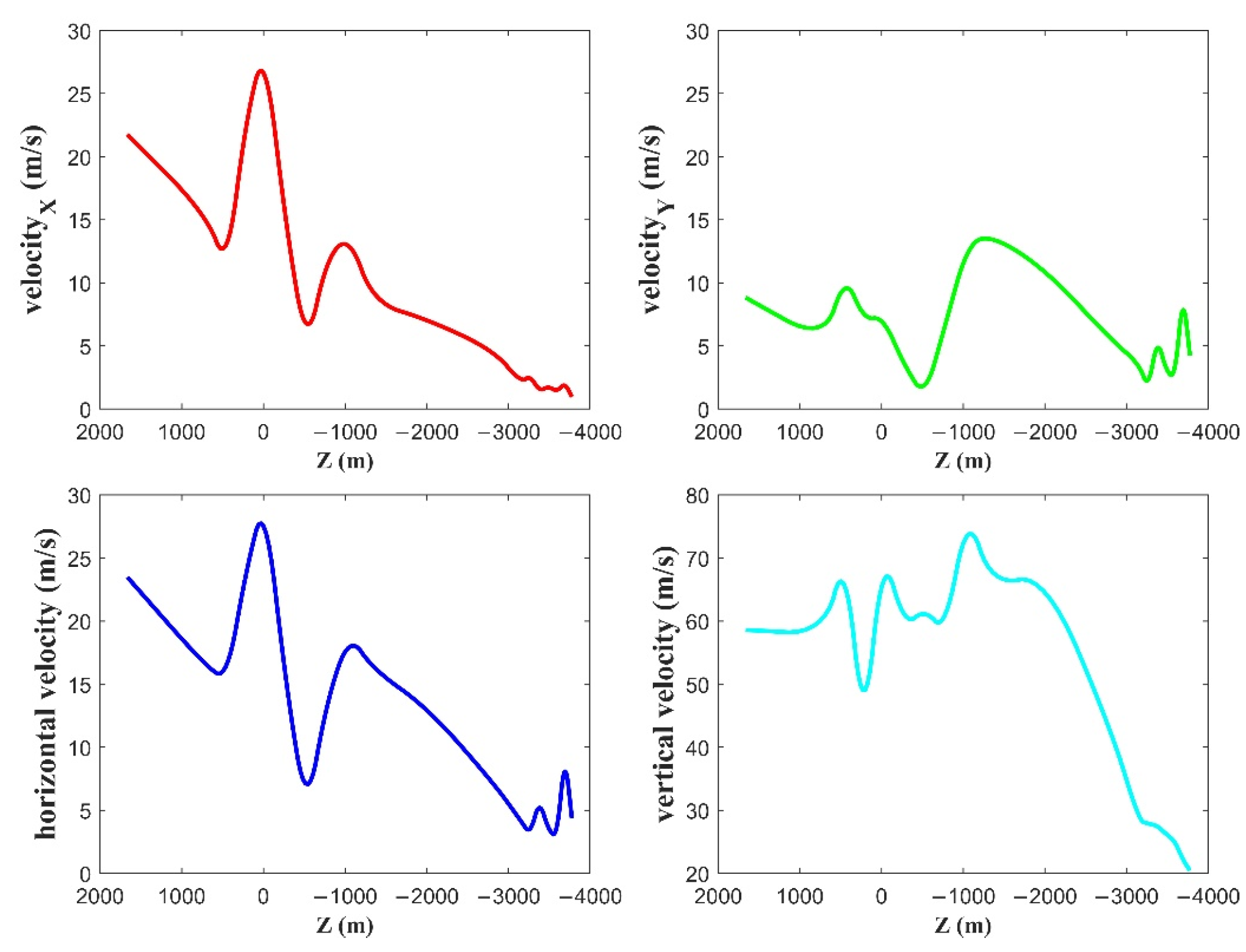
According to the translation of the landing camera, combined with the acquisition time of each descent image, the velocity components along the three directions of the coordinate axis were calculated, from which the velocity components in the XY plane (horizontal plane) were obtained, as depicted in Figure 19.
As displayed in the Figure 19, the velocity along the x-axis underwent a large fluctuation in the middle section with two extreme maximum values and two extreme minimum values, and gradually decreased to almost zero in the second half with a smooth trend. There were two extreme maximums and an extreme minimum of the velocity along the y-axis which experienced three significant decreases and two rebounds. Besides, the initial velocity along the y-axis was not as large as along the x-axis. Small fluctuations were observed at the end of the landing, presumably due to the thrust that was mostly along the y-axis. The thrust was provided by the thrusters during the auto-tuning process. From Figure 19, it can also be known that the horizontal velocity in the first half was mainly determined by the velocity along the x-axis, whereas at the end of the landing it was greatly influenced by the velocity along the y-axis. The initial velocity along the vertical direction was larger and relatively stable, reaching more than twice the initial velocity in the horizontal direction. After experiencing fluctuations in the first half, the vertical velocity reached its maximum at an altitude of about 3000 m above the surface. Then, the velocity started a rapid descent until it was about 30 m/s, during which the lander descended by an altitude of about 2000 m. At the end of the descent trajectory, a slight change in acceleration occurred as the thrusters were turned on about 1000 m above the surface, which corresponds to a velocity oscillation in the y-axis direction before landing.

4.3. Terrain Reconstruction

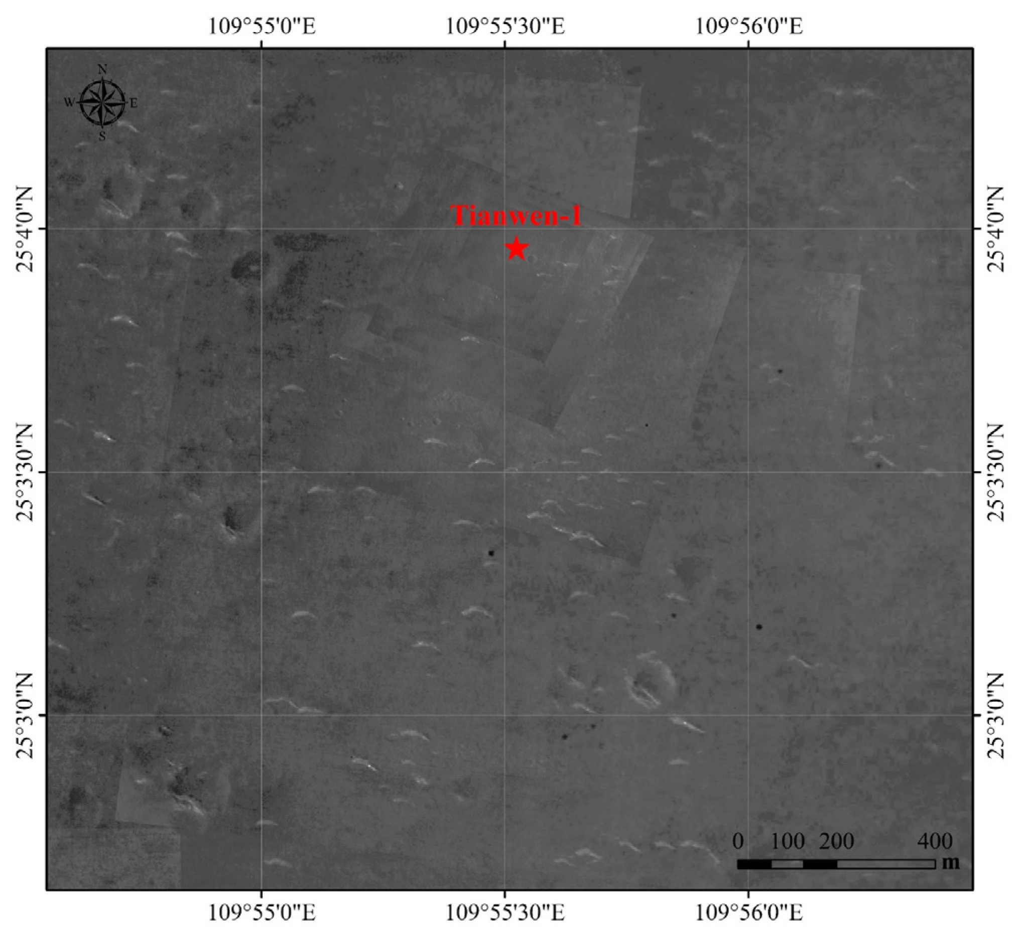
The DEM (Figure 20) and DOM (Figure 21) were reconstructed from the descent images of Tianwen-1.
This DEM of the landing area spans about 1600 m in the east–west direction, corresponding to a longitude range of about 2′, and about 1600 m in the north–south direction, corresponding to a latitude range of about 2′, which mainly contains an area of about 1200 m south of the landing site, an area of about 400 m north of the landing site, and an area of 800 m to both the west and east of the landing site. It is demonstrated that the topographic height difference in the area is within 20 m, which implies that the overall topography is relatively flat with lower terrain in the northwest and southeast areas and higher terrain in the southwest and northeast areas. The morphology of the impact crater is mainly represented by a high circular crater lip and a relatively low crater center, according to which several larger impact craters (five located in the western part with one in the eastern part as marked in Figure 20) in the landing area are clearly distinguished in the DEM. In order to evaluate the accuracy of DEM, the RMSE in the vertical direction of the control points was calculated to be 1.612 m.
To facilitate comparison with the DEM, the DOM is produced to the same extent as the DEM (Figure 21). Since the sun was located to the east of the lander during the descent process, the east side of the descent image was brighter and the west side was darker, which was most acute at the edge of the image. In addition, affected by the combination of the vignetting of the landing camera’s lens and light propagation attenuation, the descent image shows a phenomenon of brightness in the middle and darkness around, which exacerbates the problem of low illumination on the western edge of the descent image. For this reason, two templates were used for the illumination filtering of the image. Both of them are dark in the middle and bright at the periphery with the relation between light intensity and distance from the center of the template conforming to the quadratic functions. The first template is centered on the projection of the sun in the image, with the second template being centered on the center of the image. This filtering greatly attenuates but does not completely eliminate the difference in the edge’s brightness in the point cloud fusion process. As a result, some of the edges of the descent images are still visible in the DOM, which is not yet enough to interfere in the recognition of the feature’s information on Mars’ surface. As described by the DOM, there are a large number of sand ridges that mainly exist in the flat area and rarely lie inside the impact crater or across the crater lip in the landing area. The sand ridges are mainly arc-shaped, pointing from northwest to southeast with the convex direction facing north. Most of the sand ridges exist independently, whereas some of them appear to be connected. In addition, impact craters of different sizes and depths in the landing area can be clearly seen, which together with sand ridges pose a potential safety hazard to the roving rover. On this account, their effective identification will assist teleoperation departments on Earth in route planning to avoid danger.

5. Discussion and Conclusions

5.1. Discussion

In this paper, the motivation of proposing the TR-TR algorithm for dual restrained conditions comes from the mission support for Tianwen-1. When using the descent images to recover the descent trajectory and reconstruct the terrain of the landing area, various shortcomings of previous algorithms were found, thus failing to robustly recover the trajectory or reconstruct the accurate terrain. In view of this problem, this paper has made relevant research and found that there are dual restraints between the descent trajectory and the terrain of the landing area. The terrain condition in the landing area leads to the inability to calculate the motion of the landing camera robustly, and the forward motion of the landing camera along the parabolic trajectory leads to the inability to reconstruct the accurate terrain. Aiming at the problem of dual restraints, this paper studied the key technologies that can solve it, and proposed the TR-TR algorithm. The TR-TR algorithm has been verified and improved by field experiment and then applied to in-orbit data of Tianwen-1.
The advantage of the TR-TR algorithm is that it can solve the dual-restraints problem at the same time, while previous work has not been able to propose effective solutions to the dual-restraints problem, or only partial solutions to one of them. For example, data obtained by sensors were utilized to overcome the unrobustness of the trajectory recovery due to the flat terrain [19]. The plane-sweep algorithm with BSFP strategy was proposed to solve the problem of low terrain reconstruction accuracy caused by the forward motion of the landing camera [25]. Based on these works, the TR-TR algorithm made improvements for each restraint, and finally integrated them together to become an algorithm that can overcome both restraints. Thus, the TR-TR algorithm outperforms previous algorithms even when dealing with a single restraint. Some of the other previous algorithms were also tested in the field experiment. Under the condition of a single restraint in the TR-TR algorithm, the maximum error of the recovered trajectory is 0.712 m, and the accuracy is better than that of the original algorithm, but it is not as high as that of the TR-TR algorithm (0.397 m) for dual restraints [19]. The reason may be that TR-TR uses denser feature points and more accurate matching points.
The TR-TR algorithm was mainly proposed for the mission of Tianwen-1; hence, it is good at processing similar data with Tianwen-1 descent images. These kinds of descent images are sequence images, but the sampling frequency is low, which leads to the sparse images that cannot be processed according to the idea of video processing. By contrast, descent images acquired by other planet exploration missions do not necessarily have such conditions. For instance, the sensors of Chang’e-4 acquired dense descent images with high sampling frequency [27]. In addition, the descent images of Chang’e-4 have high contrast illumination since there is no air on the lunar [31]. The applicability of the TR-TR algorithm in the descent images of other planets will be better. When encountering densely sampled descent images or videos, the TR-TR algorithm will achieve higher accuracy, but also increase the computational complexity. Hence, the generality of the TR-TR algorithm still needs improvement.
The results of the field experiment showed that the TR-TR algorithm did outperform the previous methods. The TR-TR algorithm obtained refined motion with higher accuracy compared to the SIFT algorithm. This is because the TR-TR algorithm obtained uniform and dense feature points by reducing the contrast threshold. Of course, it must also have something to do with the high matching accuracy. The accuracy of refined motion is lower than that of initial motion because the cumulative error is added to it. Compared with Meng’s method [24], the TR-TR algorithm obtained more stable and higher matching accuracy after removing mismatching points. The reason for the stability is mainly because the TR-TR algorithm exploited more robust information (homography matrix and maximum height difference of the terrain), while Meng’s method exploited unstable information (fundamental matrix). More specifically, it is possible to obtain the incorrect fundamental matrix, but it is not possible to obtain the incorrect homography matrix using (quasi-) degenerated data. This is exploited by this algorithm to search for the robust homography matrix first. In fact, the homography matrix has also been combined with RANSAC to remove mismatching points [23]. However, the inlier threshold of RANSAC is not given. The threshold is explicitly given in the TR-TR algorithm based on prior terrain information. By using the DEM of the landing area, the robust maximum height difference of the landing area is known. Then, the robust homography matrix is combined with the maximum height difference to get the robust maximum plane induced parallax. Finally, matching points are checked and eliminated according to the robust maximum plane induced parallax. In addition to stability, the TR-TR algorithm also has higher matching accuracy, because the TR-TR algorithm uses the monotonicity of feature scale variation in the descent images to eliminate some other mismatching points, which is not used by Meng’s method. The field experiment of robust motion estimation mainly includes two parts: the estimation of initial motion and the adjusted motion. As for the initial value of motion, it can be seen that Meng’s method will randomly get the error solutions with the gross error when the (quasi-)degenerate data are used [24]. The error solutions come from decomposition of the incorrect fundamental matrix which is obtained randomly. In comparison, the TR-TR algorithm is able to obtain a more stable motion solution for two reasons. The first one is that the TR-TR algorithm is able to obtain two motion solutions based on the robust homography matrix decomposition and uses the parabolic property of the descent trajectory to eliminate the one that does not match the real situation, leaving the robust motion solution. The second is that according to the robust homography matrix, the TR-TR algorithm makes full use of the points outside the scene plane, and uses the epipoles constrained parallax beam method to search for a robust fundamental matrix among the matching points that may contain mismatching points. For the adjusted motion, the TR-TR algorithm is compared with the SIFT method with default threshold in OpenCV, and higher trajectory recovery accuracy is obtained. This is because the TR-TR algorithm obtains more and uniformly distributed matching points by reducing the contrast threshold of SIFT, which provides more sufficient constraints, especially for the (quasi-) degenerated data. For example, for (quasi-) degenerated data, there are points outside the scene plane, but if the number of matching points is small, it is likely to be all in the plane. However, if the number of matching points is large enough and the distribution is uniform, it is more likely to contain points outside the plane. Such a point as an observed value participating in the adjustment can provide the constraint in the vertical direction and obtain a more accurate motion solution. Compared with Meng’s algorithm [25], the TR-TR algorithm obtained higher terrain accuracy. The most direct reason is that the TR-TR algorithm found more initial seed points as exact depth constraints. The better fit of the multi-directional virtual planes to the small undulations of the terrain resulted in more initial seed points and made more ZNCC curves eligible to be the initial seed points. Meng’s method is proposed for two images, while the TR-TR algorithm is for multiple images. In the case of two images, one of the images has only one epipole, and the insensitivity of depth to parallax near the epipole cannot be resolved by more images. In contrast, in the case of multiple images, one of the images can have more than one epipole, and the insensitivity of depth recovery near a certain epipole can be solved by the sensitivity of other images in this region, thus improving the accuracy of terrain reconstruction near the epipole.
The in-orbital descent images data of Tianwen-1 were used by the TR-TR algorithm to generate the descent trajectory and reconstruct the terrain of the landing area. Some similar algorithms have been used to process in-orbit descent images of Chang’e-3 and Chang’e-4 [15,27,47]. They also successfully recovered the descent trajectory and reconstructed the terrain of landing area. The difference is that their descent trajectory is not parabolic, hence, their algorithm does not necessarily apply to Tianwen-1.

5.2. Conclusions

This paper presents a detailed description of the descent images acquired by the Tianwen-1′s landing camera and points out the difficulties encountered in the descent trajectory recovery and reconstructing terrain of the landing area using descent images in the dual-restraints conditions. In response to these difficulties, a novel trajectory recovery and terrain reconstruction (TR-TR) algorithm was proposed, which solved the problems of uneven distribution of feature points, high numbers of mismatching points owing to similar features, unrobust motion estimated from (quasi-) degenerate data, and low accuracy of terrain reconstruction in baselines along the optical axis. Robust motion was estimated by using parallax beams with epipoles constraints and utilizing parabolic characteristics of trajectories to eliminate uncertainty. More accurate trajectory was recovered by obtaining evenly distributed feature points and removing more mismatching points. More accurate and fine terrain was reconstructed by using a multi-image and multi-direction plane-sweep method with sparse spatial points. Verified by the simulated landing experiment in the Red Cliff area, the TR-TR algorithm obtained more accurate results than previous methods, including more accurate trajectories and more accurate terrain. The maximum error of recovered trajectory was reduced from 0.681 m of previous algorithm to 0.397 m. The maximum error of terrain reconstruction was reduced from the 0.692 m of previous algorithm to 0.462 m of the TR-TR algorithm. In practical applications, the TR-TR algorithm was applied to the in-orbit data of Tianwen-1 by accurately recovering the landing trajectory of the lander and mapping the high-precision terrain of the landing area. The recovered trajectory was fitted to parabola in X-axis and Y-axis directions, and the corresponding parameters and correlation coefficients were obtained. The fitting residuals were also calculated. The vertical RMSE of the reconstructed terrain in the landing area of Tianwen-1 was calculated as 1.612 m. The terrain accuracy obtained by in-orbit data is lower than that obtained by field experiment, because the accuracy of the control points in the in-orbit data is relatively lower, and the selection error of control points on the in-orbit descent image is relatively larger. The results met the accuracy requirements of the mission for terrain reconstruction and supplied a strong product to support the follow-up inspection and detection of the Zhurong rover and provided valuable data feedback for the future planetary landing mission.
The innovations of this article are as follows:
(1) A novel algorithm (TR-TR) for descent trajectory recovery and landing area terrain reconstruction based on Tianwen-1′s descent images was developed in a dual-restraints context, which has higher precision, accuracy, and robustness than previous methods;
(2) The landing simulation experiment of the Mars lander was carried out for the first time in the Mars-like landform area to verify the descent trajectory recovery and terrain reconstruction algorithms based on descent images;
(3) For the first time, the descent images of Tianwen-1 were employed to realize the recovery of the descent trajectory of the lander and the terrain reconstruction of the landing area.

5.3. Future Work

Although the TR-TR algorithm proposed in this paper has achieved good results, there are still limitations, such as the requirement of the internal parameters of the descent camera, the failure to utilize the shape and size of the ground objects in the landing area to provide scale constraints for the reconstructed terrain, and the lack of the establishment of the multi-scale precision evaluation method of terrain mapping based on images with different resolutions. Moreover, as mentioned in the discussion, the generality of the TR-TR algorithm needs to be enhanced. Further research is needed for China’s future Mars landing missions that still face enormous challenges. The terrain reconstruction algorithm based on descent images is an important prerequisite and component of point cloud based terrain reconstruction. However, dual restraints are still an inevitable problem for point cloud terrain reconstruction. Therefore, the TR-TR algorithm in this paper can also provide reference for point cloud reconstruction in planetary mapping.

Author Contributions

C.Q.: methodology, writing—original draft preparation. J.Z.: data. Y.M. and M.L.: software. S.L. and A.X.: writing—review and editing. H.Y.: experiment. Y.Y.: investigation and supervision. Y.X.: conceptualization. Y.M. and X.X. funding acquisition. All authors have read and agreed to the published version of the manuscript.

Funding

This research was funded by the National Natural Science Foundation of China (no. 42071447, 42074012 and 42030109), the Liaoning Key Research and Development Program (no. 2020JH2/10100044).

Institutional Review Board Statement

Not applicable.

Informed Consent Statement

Not applicable.

Data Availability Statement

The Tianwen-1′s orbiter data were available from Lunar and Planetary Data Release System (https://moon.bao.ac.cn/web/zhmanager/mars1). (accessed date 1 November 2021).

Acknowledgments

We would like to offer special thanks to the Beijing Institute of Spacecraft System Engineering for providing Tianwen-1′s descent images and field experiment support. We also express our gratitude to the National Astronomical Observatories, Chinese Academy of Sciences (NAOC), who supplied the Tianwen-1′s orbiter data.

Conflicts of Interest

The authors declare no conflict of interest.

References

  1. Ingersoll, A.P. Three eras of planetary exploration. Nat. Astron. 2017, 1, 10. [Google Scholar] [CrossRef] [Green Version]
  2. Binzel, R.P. A golden spike for planetary science. Science 2012, 338, 203–204. [Google Scholar] [CrossRef] [PubMed]
  3. Wang, J.; Zhang, Y.; Di, K.C.; Chen, M.; Duan, J.F.; Kong, J.; Xie, J.F.; Liu, Z.Q.; Wan, W.H.; Rong, Z.F.; et al. Localization of the Chang’e-5 Lander Using Radio-Tracking and Image-Based Methods. Remote Sens. 2021, 13, 590. [Google Scholar] [CrossRef]
  4. Li, C.; Wang, C.; Wei, Y.; Lin, Y. China’s present and future lunar exploration program. Science 2019, 365, 238–239. [Google Scholar] [CrossRef] [PubMed]
  5. Yang, P.; Huang, Y.; Li, P.; Liu, S.; Shan, Q.; Zheng, W. Trajectory Determination of Chang’E-5 during Landing and Ascending. Remote Sens. 2021, 13, 4837. [Google Scholar] [CrossRef]
  6. Jiang, X.; Yang, B.; Li, S. Overview of China’s 2020 Mars mission design and navigation. Astrodynamics 2018, 2, 1–11. [Google Scholar] [CrossRef]
  7. Wan, W.X.; Wang, C.; Li, C.L.; Wei, Y. China’s first mission to Mars. Nat. Astron. 2020, 4, 721. [Google Scholar] [CrossRef]
  8. Wan, W.; Yu, T.; Di, K.; Wang, J.; Liu, Z.; Li, L.; Liu, B.; Wang, Y.; Peng, M.; Bo, Z. Visual Localization of the Tianwen-1 Lander Using Orbital, Descent and Rover Images. Remote Sens. 2021, 13, 3439. [Google Scholar] [CrossRef]
  9. Ground Research and Application System of China’s Lunar and Planetary Exploration Program. Tianwen-1 Middle Resolution Imaging Camera Dataset; China National Space Administration: Beijing, China, 2020. [Google Scholar]
  10. Ground Research and Application System of China’s Lunar and Planetary Exploration Program. Tianwen-1 High Resolution Imaging Camera Dataset; China National Space Administration: Beijing, China, 2020. [Google Scholar]
  11. Kirk, R.L.; Mayer, D.P.; Fergason, R.L.; Redding, B.L.; Galuszka, D.M.; Hare, T.M.; Gwinner, K. Evaluating Stereo Digital Terrain Model Quality at Mars Rover Landing Sites with HRSC, CTX, and HiRISE Images. Remote Sens. 2021, 13, 3511. [Google Scholar] [CrossRef]
  12. Huang, X.; Li, M.; Wang, X.; Hu, J.; Zhao, Y.; Guo, M.; Xu, C.; Liu, W.; Wang, Y.; Hao, C.; et al. The Tianwen-1 Guidance, Navigation, and Control for Mars Entry, Descent, and Landing. Space Sci. Technol. 2021, 2021, 9846185. [Google Scholar] [CrossRef]
  13. Peng, M.; Di, K.; Wang, Y.; Wan, W.; Liu, Z.; Wang, J.; Li, L. A Photogrammetric-Photometric Stereo Method for High-Resolution Lunar Topographic Mapping Using Yutu-2 Rover Images. Remote Sens. 2021, 13, 2975. [Google Scholar] [CrossRef]
  14. Chen, Z.; Jiang, J. Crater Detection and Recognition Method for Pose Estimation. Remote Sens. 2021, 13, 3467. [Google Scholar] [CrossRef]
  15. Liu, Z.; Di, K.; Peng, M.; Wan, W.; Liu, B.; Li, L.; Yu, T.; Wang, B.; Zhou, J.; Chen, H. High precision landing site mapping and rover localization for Chang’e-3 mission. Sci. China Phys. Mech. Astron. 2015, 58, 1–11. [Google Scholar] [CrossRef]
  16. Yan, R.; Cao, Z.; Wang, J.; Zhong, S.; Klein, D.; Cremers, A. Horizontal velocity estimation via downward looking descent images for lunar landing. IEEE Trans. Aerosp. Electron. Syst. 2014, 50, 1197–1221. [Google Scholar] [CrossRef]
  17. Johnson, A.; Willson, R.; Cheng, Y.; Goguen, J.; Leger, C.; Sanmartin, M.; Matthies, L. Design through operation of an image-based velocity estimation system for mars landing. Int. J. Comput. Vis. 2007, 74, 319–341. [Google Scholar] [CrossRef]
  18. Cheng, Y.; Goguen, J.; Johnson, A.; Leger, C.; Matthies, L.; San Martin, M.; Willson, R. The Mars exploration rovers descent image motion estimation system. IEEE Intell. Syst. 2004, 19, 13–21. [Google Scholar] [CrossRef]
  19. Xiong, Y.; Olson, C.F.; Matthies, L.H. Computing depth maps from descent images. Mach. Vis. Appl. 2005, 16, 139–147. [Google Scholar] [CrossRef]
  20. Olson, C.; Matthies, L.; Xiong, Y.; Li, R.; Ma, F. Multi-Resolution Mapping Using Surface, Descent and Orbit Images; Jet Propulsion Laboratory: Pasadena, CA, USA, 2001. [Google Scholar]
  21. Fischler, M.A.; Bolles, R.C. Random sample consensus: A paradigm for model fitting with applications to image analysis and automated cartography. Commun. ACM (USA) 1981, 24, 381–395. [Google Scholar] [CrossRef]
  22. Andrew, A.M. Multiple view geometry in computer vision. Kybernetes 2001, 30, 1333–1341. [Google Scholar]
  23. Li, M.; Liu, S.; Ma, Y.; Sun, C.; Jia, Y. Descent image based landing area terrain reconstruction technology for lunar landing mission. Imaging Sci. J. 2015, 63, 440–446. [Google Scholar] [CrossRef]
  24. Meng, C.; Zhou, N.; Xue, X.L.; Jia, Y. Homography-based depth recovery with descent images. Mach. Vis. Appl. 2013, 24, 1093–1106. [Google Scholar] [CrossRef]
  25. Meng, C.; Zhou, N.; Jia, Y. Improved best match search method in depth recovery with descent images. Mach. Vis. Appl. 2015, 26, 251–266. [Google Scholar] [CrossRef]
  26. Xu, X.C.; Zheng, Z.Z.; Xu, A.G.; Liu, S.C. An Optimized Method for Terrain Reconstruction Based on Descent Images. J. Eng. Technol. Sci. 2016, 48, 31–48. [Google Scholar] [CrossRef] [Green Version]
  27. Liu, J.J.; Ren, X.; Yan, W.; Li, C.L.; Zhang, H.; Jia, Y.; Zeng, X.G.; Chen, W.L.; Gao, X.Y.; Liu, D.W.; et al. Descent trajectory reconstruction and landing site positioning of Chang’E-4 on the lunar farside. Nat. Commun. 2019, 10, 4229. [Google Scholar] [CrossRef] [Green Version]
  28. Di, K.; Liu, Z.; Liu, B.; Wan, W.; Peng, M.; Wang, Y.; Gou, S.; Yue, Z.; Xin, X.; Jia, M.; et al. Chang’e-4 lander localization based on multi-source data. J. Remote Sens. 2019, 23, 177–184. [Google Scholar]
  29. Di, K.; Liu, Z.; Liu, B.; Wan, W.; Peng, M.; Li, J.; Xie, J.; Jia, M.; Niu, S.; Xin, X. Topographic Analysis of Chang’e-4 Landing Site Using Orbital, Descent and Ground Data. Int. Arch. Photogramm. Remote Sens. Spatial Inf. Sci. 2019, XLII-2/W13, 1383–1387. [Google Scholar] [CrossRef] [Green Version]
  30. Liu, Z.Q.; Di, K.C.; Li, J.; Xie, J.F.; Cui, X.F.; Xi, L.H.; Wan, W.H.; Peng, M.; Liu, B.; Wang, Y.X.; et al. Landing site topographic mapping and rover localization for Chang’e-4 mission. Sci. China-Inf. Sci. 2020, 63, 140901. [Google Scholar] [CrossRef] [Green Version]
  31. Wan, W.; Liu, Z.; Liu, B.; Di, K.; Wang, J.; Liu, C.; Yu, T.; Miao, Y.; Peng, M.; Wang, Y.; et al. Descent trajectory recovery of Chang’e-4 lander based on descent images. Int. Arch. Photogramm. Remote Sens. Spatial Inf. Sci. 2019, XLII-2/W13, 1457–1461. [Google Scholar] [CrossRef] [Green Version]
  32. Lowe, D.G. Distinctive image features from scale-invariant keypoints. Int. J. Comput. Vis. 2004, 60, 91–110. [Google Scholar] [CrossRef]
  33. Bay, H.; Ess, A.; Tuytelaars, T.; Van Gool, L. Speeded-Up Robust Features (SURF). Comput. Vis. Image Underst. 2008, 110, 346–359. [Google Scholar] [CrossRef]
  34. Leutenegger, S.; Chli, M.; Siegwart, R.Y. BRISK: Binary Robust Invariant Scalable Keypoints. In Proceedings of the IEEE International Conference on Computer Vision (ICCV), Barcelona, Spain, 6–13 November 2011; pp. 2548–2555. [Google Scholar]
  35. Tareen, S.A.K.; Saleem, Z. A comparative analysis of sift, surf, kaze, akaze, orb, and brisk. In Proceedings of the 2018 International Conference on Computing, Mathematics and Engineering Technologies (iCoMET), Sukkur, Pakistan, 3–4 March 2018; pp. 1–10. [Google Scholar]
  36. Suju, D.A.; Jose, H. FLANN: Fast Approximate Nearest Neighbour Search Algorithm for elucidating Human-Wildlife conflicts in Forest areas. In Proceedings of the 4th International Conference on Signal Processing, Communication and Networking (ICSCN), Chennai, India, 16–18 March 2017. [Google Scholar]
  37. Guo, G.D.; Wang, H.; Bell, D.; Bi, Y.X.; Greer, K. KNN model-based approach in classification. In On the Move to Meaningful Internet Systems 2003: Coopis, Doa, and Odbase; Meersman, R., Tari, Z., Schmidt, D.C., Eds.; Lecture Notes in Computer Science; Springer: Berlin/Heidelber, Germany, 2003; Volume 2888, pp. 986–996. [Google Scholar]
  38. Rebert, M.; Monnin, D.; Bazeille, S.; Cudel, C. Parallax beam: A vision-based motion estimation method robust to nearly planar scenes. J. Electron. Imaging 2019, 28, 023030. [Google Scholar] [CrossRef]
  39. Frahm, J.; Pollefeys, M. RANSAC for (Quasi-)Degenerate data (QDEGSAC). In Proceedings of the 2006 IEEE Computer Society Conference on Computer Vision and Pattern Recognition (CVPR’06), New York, NY, USA, 17–22 June 2006; pp. 453–460. [Google Scholar]
  40. Decker, P.; Paulus, D.; Feldmann, T. Dealing with degeneracy in essential matrix estimation. In Proceedings of the 15th IEEE International Conference on Image Processing (ICIP 2008), San Diego, CA, USA, 12–15 October 2008; pp. 1964–1967. [Google Scholar]
  41. Chum, O.; Werner, T.; Matas, J. Two-view geometry estimation unaffected by a dominant plane. In Proceedings of the Conference on Computer Vision and Pattern Recognition, San Diego, CA, USA, 20–25 June 2005; pp. 772–779. [Google Scholar]
  42. Torr, P.H.S. An assessment of information criteria for motion model selection. In Proceedings of the 1997 IEEE Computer Society Conference on Computer Vision and Pattern Recognition (Cat. No.97CB36082), San Juan, Puerto Rico, 17–19 June 1997; pp. 47–52. [Google Scholar] [CrossRef]
  43. Collins, R.T. A space-sweep approach to true multi-image matching. In Proceedings of the 1996 IEEE Computer Society Conference on Computer Vision and Pattern Recognition (Cat. No.96CB35909), San Francisco, CA, USA, 18–20 June 1996; pp. 358–363. [Google Scholar] [CrossRef]
  44. Moulon, P.; Monasse, P.; Marlet, R. Adaptive Structure from Motion with a Contrario Model Estimation. Computer Vision–ACCV 2012. In Proceedings of the 11th Asian Conference on Computer Vision, Daejeon, Korea, 5–9 November 2012; Revised Selected Papers, 2013. pp. 257–270. [Google Scholar] [CrossRef] [Green Version]
  45. Malis, E.; Vargas, M. Deeper Understanding of the Homography Decomposition for Vision-Based Control; INRIA: Le Chesnay-Rocquencourt, France, 2007; p. 90.
  46. Chen, L.; Xu, Y.; Li, B. Comparitive Study of the Geomorphological Characteristics of Valley Networks between Mars and the Qaidam Basin. Remote Sens. 2021, 13, 4471. [Google Scholar] [CrossRef]
  47. Jia, Y.; Liu, S.; Li, M.; Li, Q.; Peng, S.; Wen, B.; Ma, Y.; Zhang, S. Chang’E-3 system pinpoint landing localization based on descent image sequence. Chin. Sci. Bull. 2014, 59, 1838–1843. [Google Scholar]
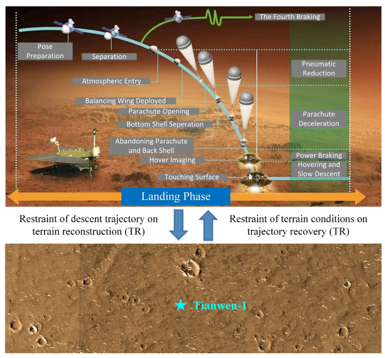
Figure 1. The Dual-Restraints of Trajectory Recovery and Terrain Reconstruction (Material comes from the China Academy of Space Technology, CAST, Beijing, China).
Remotesensing 14 00709 g001
Figure 2. Flow chart for TR-TR processing the descent images of Tianwen-1.
Remotesensing 14 00709 g002
Figure 3. Plane induced parallax. The ray through X intersects the plane π at the point X π . The images of X and X π are coincident points at x in the first view. In the second view, the images are the points x and x ˜ = H x , respectively. These points are not coincident when X is not on π , but both are on the epipolar line l x of x . The vector between the points x and x ˜ is the parallax relative to the homography induced by the plane π .
Remotesensing 14 00709 g003
Figure 4. The locations of O H a and O H b when O L is fixed.
Remotesensing 14 00709 g004
Figure 5. The locations of O H a and O H b with two surfaces overlapping.
Remotesensing 14 00709 g005
Figure 6. The ground control points are represented by blue dots and white numbers, and the landing point is indicated by a red pentagram.
Remotesensing 14 00709 g006
Figure 7. DEM of the experimental area.
Remotesensing 14 00709 g007
Figure 8. Comparison of matching accuracy between the methods of this paper and Meng’s.
Remotesensing 14 00709 g008
Figure 9. Comparison of the initial motion estimation results of image pairs between the methods of this paper and Meng’s. (a) Comparison of normalized horizontal error. (b) Comparison of pitch error. (c) Comparison of roll error. (d) Comparison of yaw error.
Remotesensing 14 00709 g009
Figure 10. The comparison of extracted feature points between two methods shown in selected descent image.
Remotesensing 14 00709 g010
Figure 11. Comparison of the refined motion of selected images after bundle adjustment using feature points extracted by the methods of this paper and SIFT. (a) Comparison of normalized horizontal error. (b) Comparison of pitch error. (c) Comparison of roll error. (d) Comparison of yaw error.
Remotesensing 14 00709 g011
Figure 12. Comparison of the number of initial seed points between methods of this paper and Meng’s.
Remotesensing 14 00709 g012
Figure 13. Comparison of depth error maps between methods of this paper and Meng’s.
Remotesensing 14 00709 g013
Figure 14. The blue part of the figure shows the deep map errors obtained by this paper’s method (marked as E T R T R ) and Meng’s method (marked as E M e n g ), respectively. The red part indicates the normalized difference (marked as d E ) between E T R T R and E M e n g by the equation: d E = 1 E T R T R / E M e n g . The normalized difference ( d E ) reflects the advantage of the method proposed in this paper.
Remotesensing 14 00709 g014
Figure 15. Footprint map of Tianwen-1′s descent images.
Remotesensing 14 00709 g015
Figure 16. Diagram of the distribution of the ground control points selected for Tianwen-1.
Remotesensing 14 00709 g016
Figure 17. Side views of the descent trajectory of the Tianwen-1′s landing camera with the left picture viewed from west to east and the right picture viewed from south to north. The quadratic curves in two directions are fitted respectively.
Remotesensing 14 00709 g017
Figure 18. Top view of the descent trajectory of Tianwen-1′s landing camera. The green dots indicate the landing camera positions corresponding to the descent images, whereas the solid orange line represents the descent trajectory.
Remotesensing 14 00709 g018
Figure 19. Velocity curve of the landing camera of Tianwen-1.
Remotesensing 14 00709 g019
Figure 20. DEM of the landing area of Tianwen-1, and the impact craters are marked as red dashed circles.
Remotesensing 14 00709 g020
Figure 21. DOM of the landing area of Tianwen-1.
Remotesensing 14 00709 g021
Table 1. Landing camera parameters.
NameValue
Diagonal field of view (FOV)43°
Square FOV30° × 30°
Focal length20 mm
Spectral range500~800 nm
Entrance pupil diameter≥4 mm
Entrance pupil position21.9 mm
Integral time0.03~64 ms
Image area resolution2048 × 2048
Pixel size5.5 μm
Table 2. Acquisition times of the descent images.
Image IDAcquisition Time (s)Image IDAcquisition Time (s)
23T23 + 0.00033T23 + 65.536
24T23 + 28.67234T23 + 81.273
25T23 + 32.76835T23 + 94.209
26T23 + 36.86436T23 + 98.305
27T23 + 40.96037T23 + 102.401
28T23 + 45.05638T23 + 106.497
29T23 + 49.15239T23 + 110.593
30T23 + 53.24840T23 + 114.689
31T23 + 57.34441T23 + 118.785
32T23 + 61.44042T23 + 122.881
Table 3. Number of feature tracks obtained by SIFT and the method of this paper.
Length of Feature TracksSIFTThe Method of This Paper
211052176
37723680
43834262
5342997
671821
70782
80215
9016
Table 4. Residual error in the X-axis direction and Y-axis direction.
Z (m)Res in X-axis (m)Res in Y-axis (m)Z (m)Res in X-axis (m)Res in Y-axis (m)
2508.252 8.213 3.935 −1482.290 5.689 8.766
828.214 −8.655 −0.465 −2542.272 6.976 0.182
591.026 −8.452 −0.334 −3094.474 0.944 −1.198
301.692 −1.730 −3.466 −3210.715 0.092 −5.491
130.631 −3.613 −8.914 −3324.941 −0.003 −1.711
−161.540 −0.994 −6.517 −3437.747 −0.582 −2.156
−404.045 −2.488 −2.847 −3545.003 −0.247 −0.095
−657.444 4.802 3.305 −3647.823 −1.170 2.323
−896.076 3.575 5.838 −3738.504 −2.928 0.689
−1213.155 4.299 7.291 −3822.342 −3.728 0.865
Table 5. RMSE and coefficient of determination in the X-axis direction and Y-axis direction.
Statistic VariateX-axisY-axis
RMSE (m) 4.458 4.351
Coefficient of Determination0.903 0.967
Publisher’s Note: MDPI stays neutral with regard to jurisdictional claims in published maps and institutional affiliations.