
Supervised Machine Learning Approaches on Multispectral Remote Sensing Data for a Combined Detection of Fire and Burned Area


Abstract
:1. Introduction
- Combined detection of active fire and burned area: We focused on detecting active fires and burned areas in one, combined data-driven approach. In existing studies, different approaches have been used for the two sub-tasks [15], if a distinction was performed between burned area and active fire. We developed a methodology to detect active fires and burned areas in one go using the same ML approach for both sub-tasks;
- Configuration of a generic concept: The concept is setup to enable a generic detection of fire areas and burned areas. Thus, we can distinguish fire and burned area incidents worldwide on an appropriate scale with the given methodological approach independently of prior or detailed knowledge of the appearance of either class in the investigated region. This novel workflow enables facile detection of both relevant areas in one go, which can be used for further risk management or other applications;
- Selection of appropriate ML approaches: Many ML approaches would be eligible to carry out the task of fire and burned area detection. We investigated and evaluated the applicability of several ML approaches and selected the best-performing for a possible application;
- Generation of reference data: Reference data are required for the training and testing steps of ML approaches. Since appropriate reference data were not available for active fires nor burned areas, large-scale reference data were generated. This generation was also set up as a generic concept that can be used for reference data manufacturing in any fire and burned area detection application worldwide;
- Detection at a high spatial resolution: For subsequent risk analysis, fire and burned area detection needs to be possible with very high accuracy, requiring a high spatial resolution of the chosen satellite data. Several types of remote sensing data can be used, but we relied on optical remote sensing data since they generally provide a higher spatial resolutions than, for example, thermal data [16]. The analysis was accomplished with the use of Sentinel-2 data, which provide a spatial resolution of 10 m in several bands [15]. With a spatial resolution of 10 m, we can ensure a much more accurate prediction of fires and burned areas affecting structures (such as roads) in these small dimensions.
1.1. Research Background

| Sensor | Methodological Approach | Satellite Data and Studies |
|---|---|---|
| Thermal | Thresholding | ASTER [11], AVHHR [33], NOAA-N [34] |
| Contextual Approach | Himawari-8 [35], AVHHR [36] | |
| Thresholding and Contextual Approach | MODIS [21,37], VIIRS [16], SEVIRI [38], theoretical [39] | |
| Anomaly Detection | GOES [40] | |
| Optical | Thresholding | Landsat-8 [10,23] |
| Contextual Approach | ASTER [24] |
| Sensor | Methodological Approach | Satellite Data and Studies |
|---|---|---|
| SAR | Index-Based | RADARSAT-2 [25], Envisat ASAR [41] |
| Change Detection | ERS-2 [26,42] | |
| Unsupervised Classification | RADARSAT-2 [43] | |
| Image Segmentation | PALSAR [44] | |
| Supervised Classification | RADARSAT-2 [43] | |
| Unsupervised Classification | Sentinel-1 [45] | |
| Thermal-Optical | Bayesian Algorithm | MODIS [9] |
| Adaptive Classification | MODIS [46] | |
| Thermal | Via Active Fire/Multitemporal | MODIS [47] |
| Via Active Fire | VIIRS [18] | |
| Optical | Index-Based | Sentinel-2 [30], Landsat-4/-5/-7 [48,49], Landsat-8 [27] |
| Index-Based + Contextual | Sentinel-2 [50], Landsat-4/-5/-7 [51], Landsat-8 [50,52], MODIS [53] | |
| Object-Based | AVHRR [29], ASTER [28], Sentinel-2 [5,50], Landsat-4/-5 [54], Landsat-8 [50,55] | |
| Via Active Fire + SVM | PROBA-V [14] | |
| Comparison of Methods | Landsat [56] | |
| Supervised Classification | Landsat-5 [57,58], Sentinel-2 [31,59] | |
| Change Detection | SPOT [19] | |
| Combination | Index-Based | MODIS/Landsat-7/-8 [8] |
| Bayesian Updating of Land Cover | Landsat-8/Sentinel-2/MODIS [12] | |
| Supervised Classification | Sentinel-1/-2/-3/MODIS [32] |
| Sensor | Methodological Approach | Satellite Data and Studies |
|---|---|---|
| Optical | Index-Based | Landsat-8/Sentinel-2 [15] |
| Combination | Thresholding | MIVIS [60] |
| Comparison of Methods | Theoretical [3] |
1.2. Subsumption of Our Study
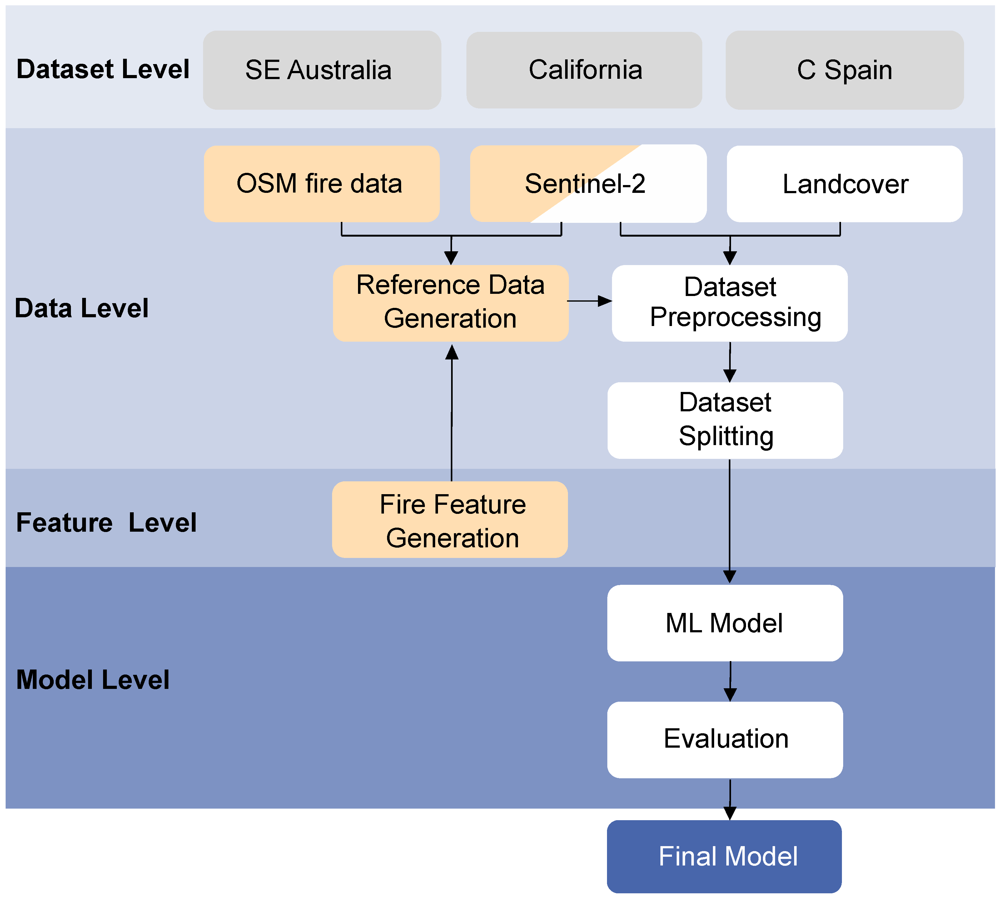
2. Datasets and Methodology
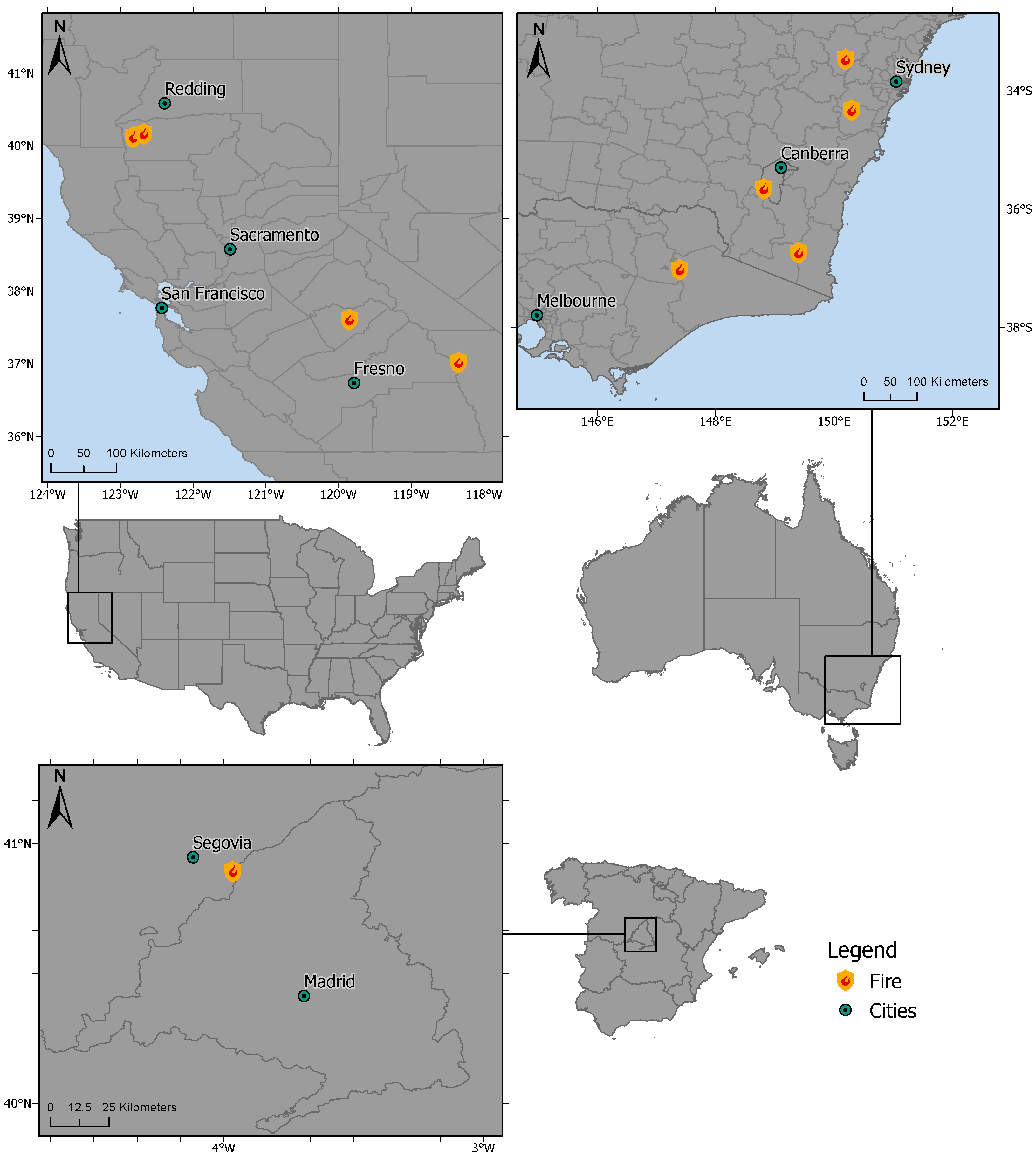
2.1. Selected Study Regions
2.2. Data Basis, Generated Datasets, and Their Preparation
2.2.1. Input Features
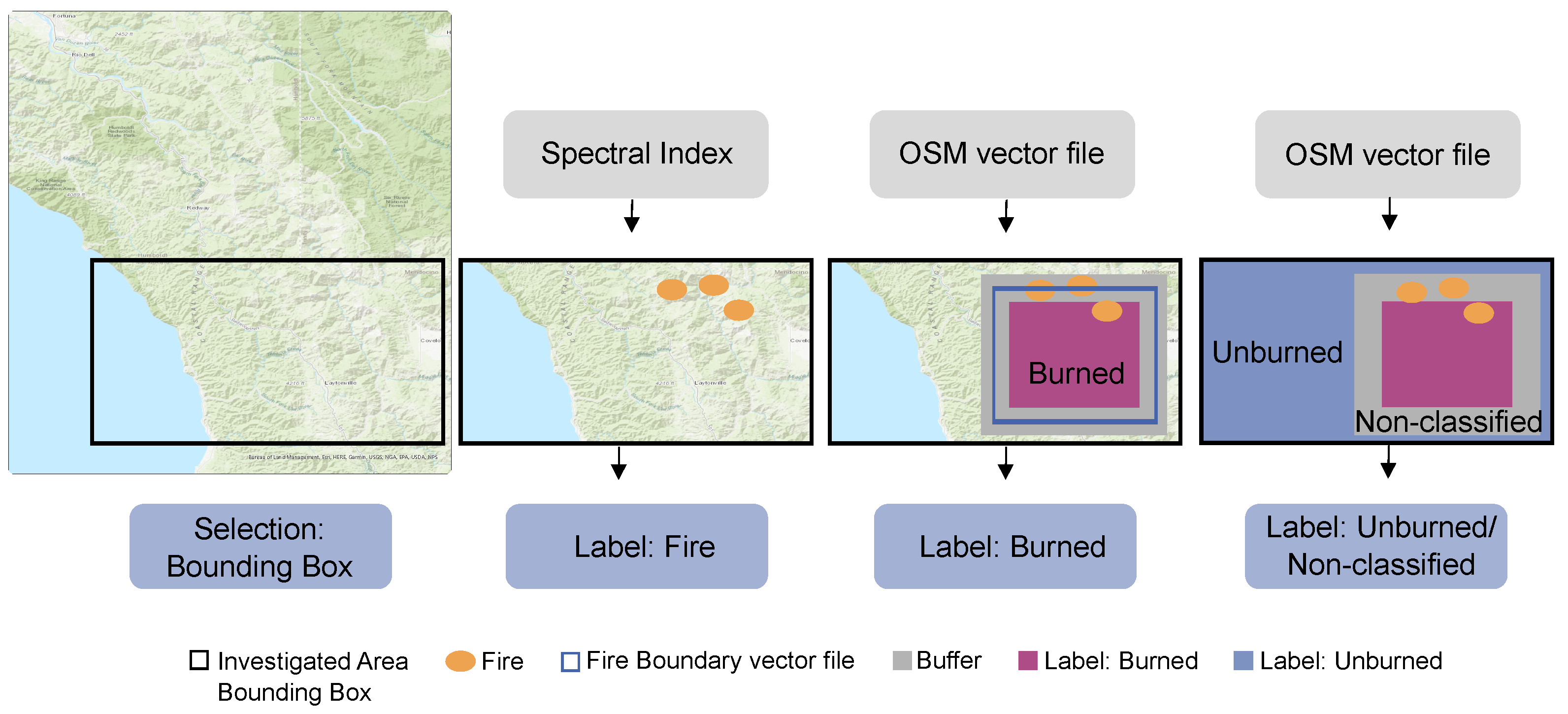
2.2.2. Generated Reference Data
- 1.
- Select a specific region of interest inside the study region (Section 2.1) by applying a bounding box, for which information on burned and unburned areas provided by OSM data is available;
- 2.
- Detect an active fire area based on spectral indices. The detected pixels are labeled as Fire;
- 3.
- Detect a burned area based on OSM data. The detected pixels are labeled as Burned;
- 4.
- Finally, label the rest (neither fire nor burned) of the pixels within the bounding box as Unburned or Non-classified.
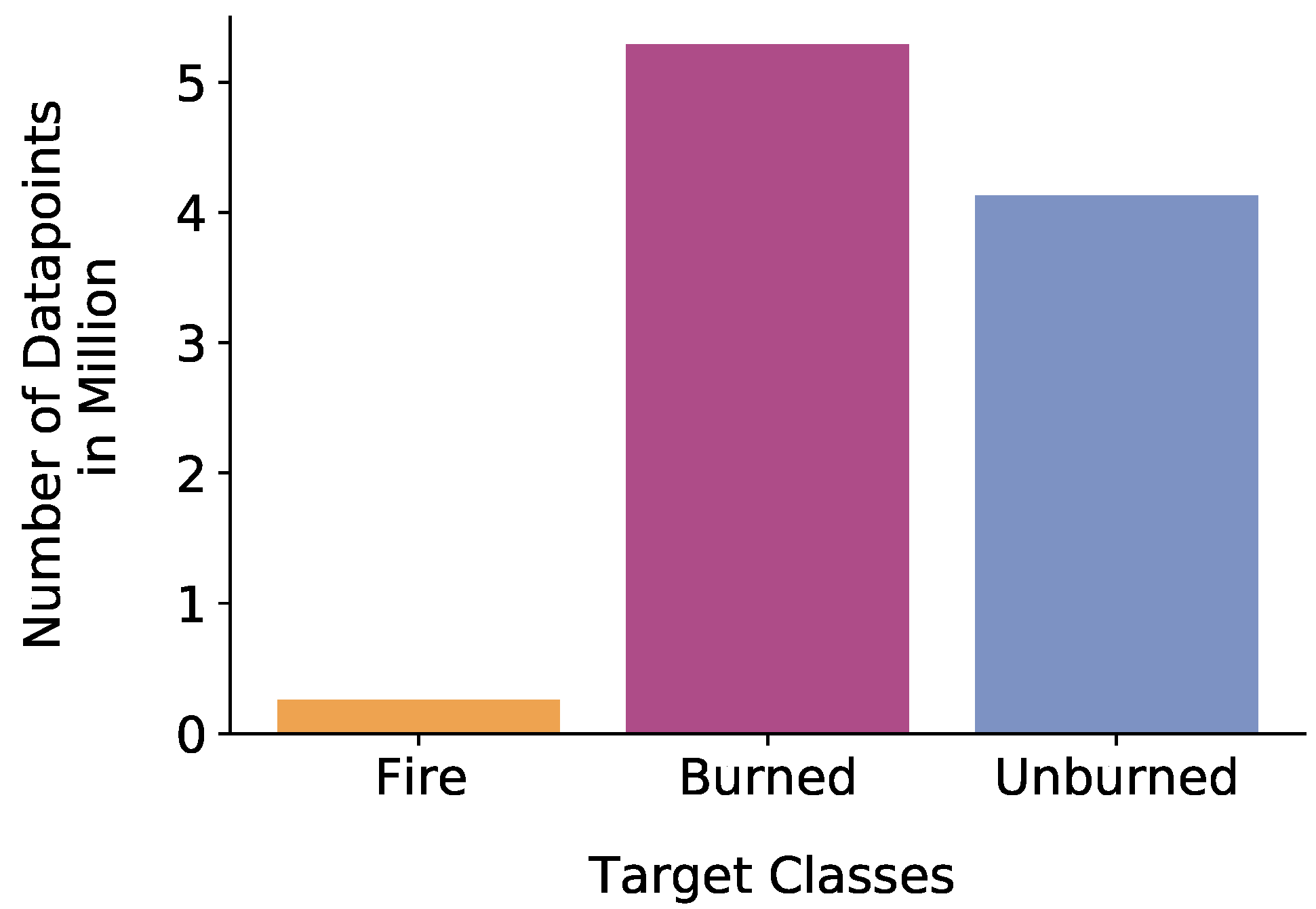
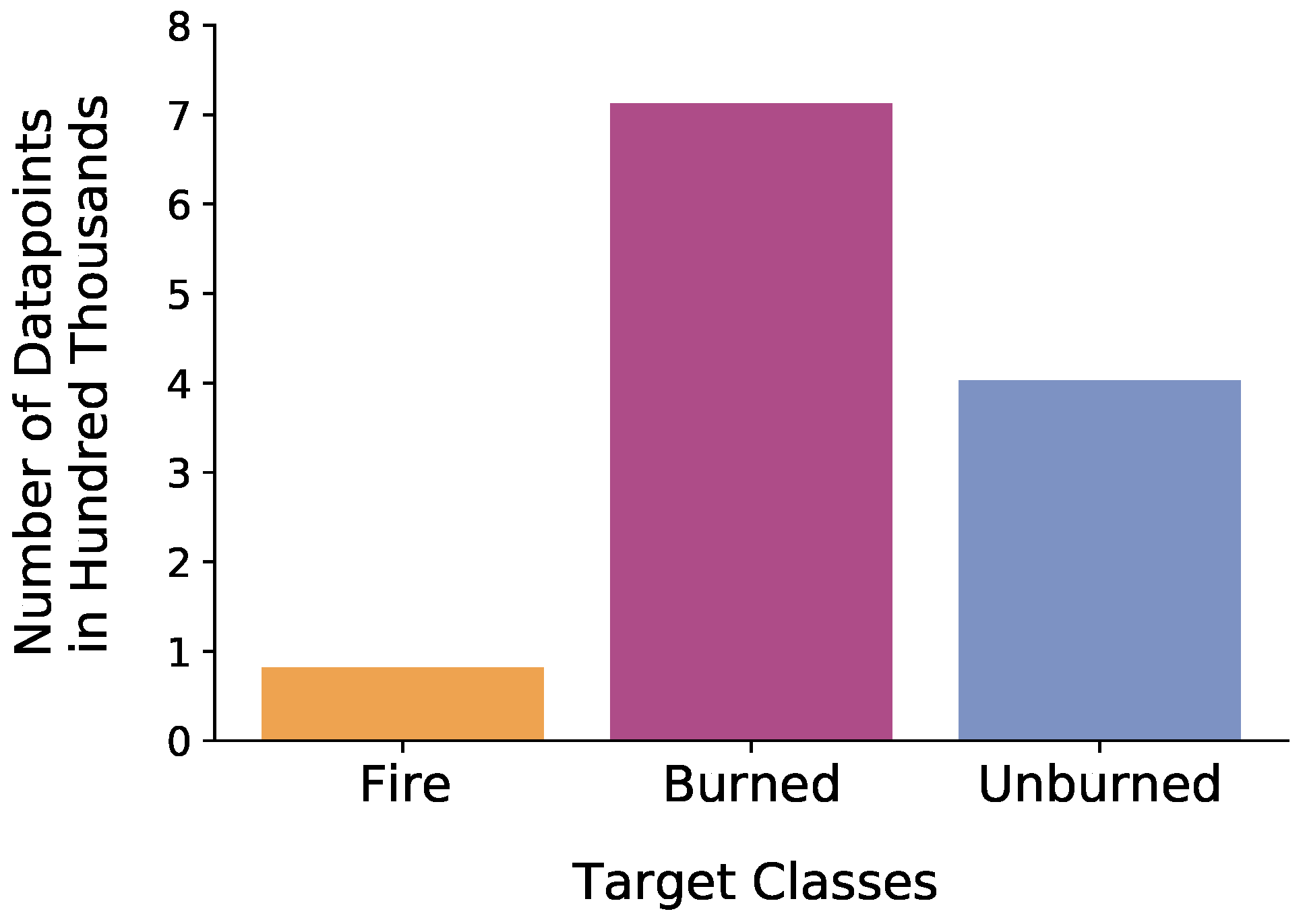
2.2.3. Dataset and Imbalance
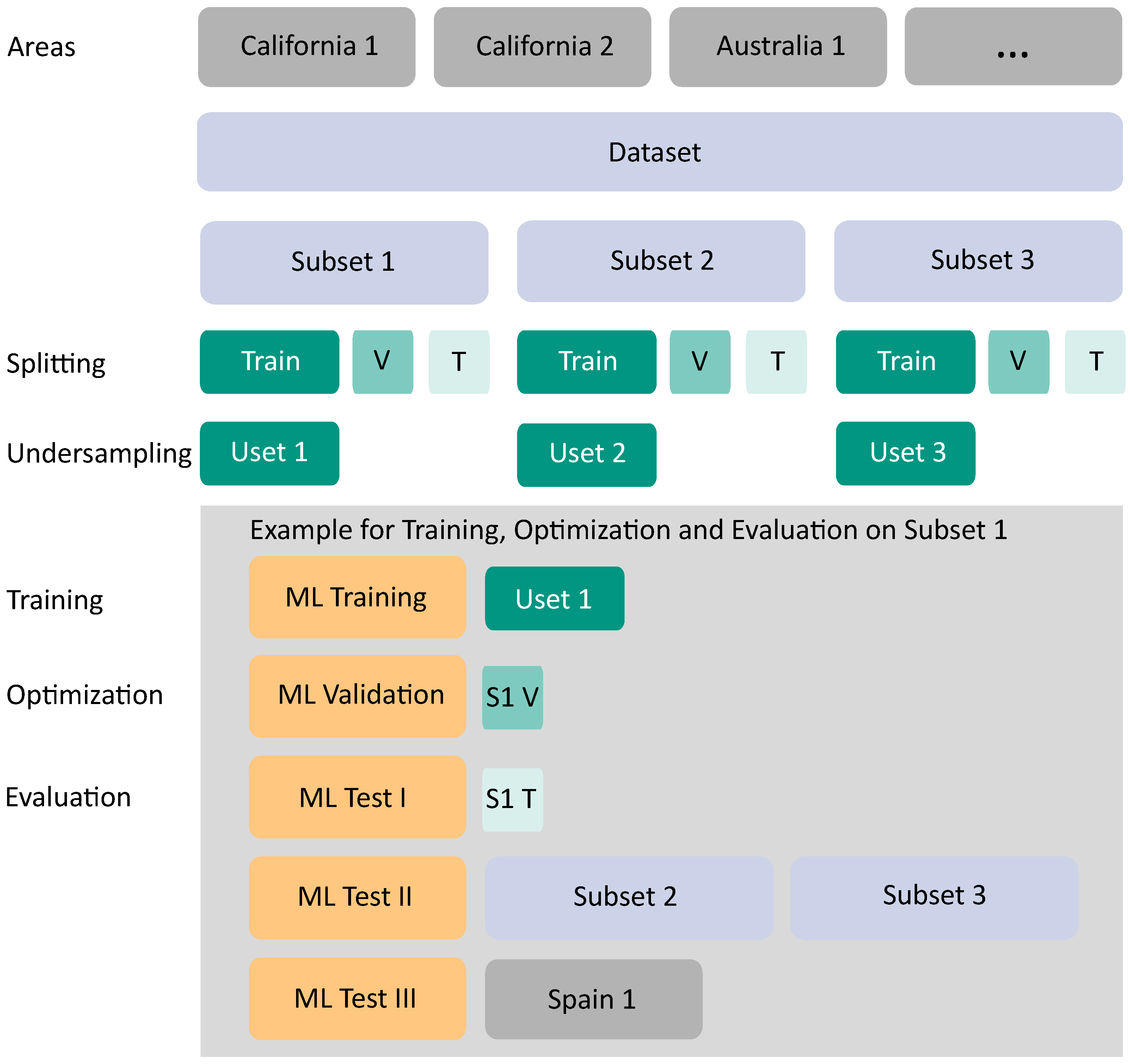
2.2.4. Dataset Preparation, Splitting, and Undersampling
- The Uset was used for training the ML approach, and the validation was conducted with the validation set of the respective subset;
- Then, Test I testing was conducted with the test set of the respective subset;
- The total of the two other subsets was used as further test data in Test II. For example, in the case of Uset 1, Subset 2 and Subset 3 were used as test datasets;
- For a completely independent evaluation in Test III, the dataset created for the selected region of Spain, in the training and testing steps a so-far unseen region, served as an additional test set.
2.3. Methods
2.3.1. Machine Learning Models for Classification
2.3.2. Accuracy Assessment
- OA represents the proportion of correctly classified test data points among all other data points and is calculated according to Equation (2).
- measures the agreement between two raters, each f which classifies each data point. It is considered a more robust measure since it considers the possibility of agreement occurring by chance. The two terms included in Equation (3) are the observed agreement among the raters (which is the above-mentioned overall accuracy (OA)) and the hypothetical probability of agreement by chance .where:and represent the sum of the products of the row total and the column total sum of each class, which can be calculated by summing the row and column values for each class in the confusion matrix;
- Precision (also correctness) predicts the positive values.
- Recall (also completeness) rates the TP and is necessary to calculate the F1-Score. Note that we excluded the recall in the Results Section (see Section 3).
- AA equals the weighted Recall in a multi-class classification problem. We therefore only included the AA in the Results Section (see Section 3). The weighted Recall is calculated from the classwise Recall calculated in the earlier step;
- The F1-Score is a metric of the test’s accuracy. It considers the Precision and Recall of the test subset to compute the harmonic mean.
- BA gives information about how well a class is classified by the respective ML model. Moreover, it is class imbalance suitable since it takes into account the individual classes’ sizes [89].where is the true label of the i-th data point, is the corresponding weight, and is the predicted class label.
3. Results
3.1. Overall Classification Performance of the Models
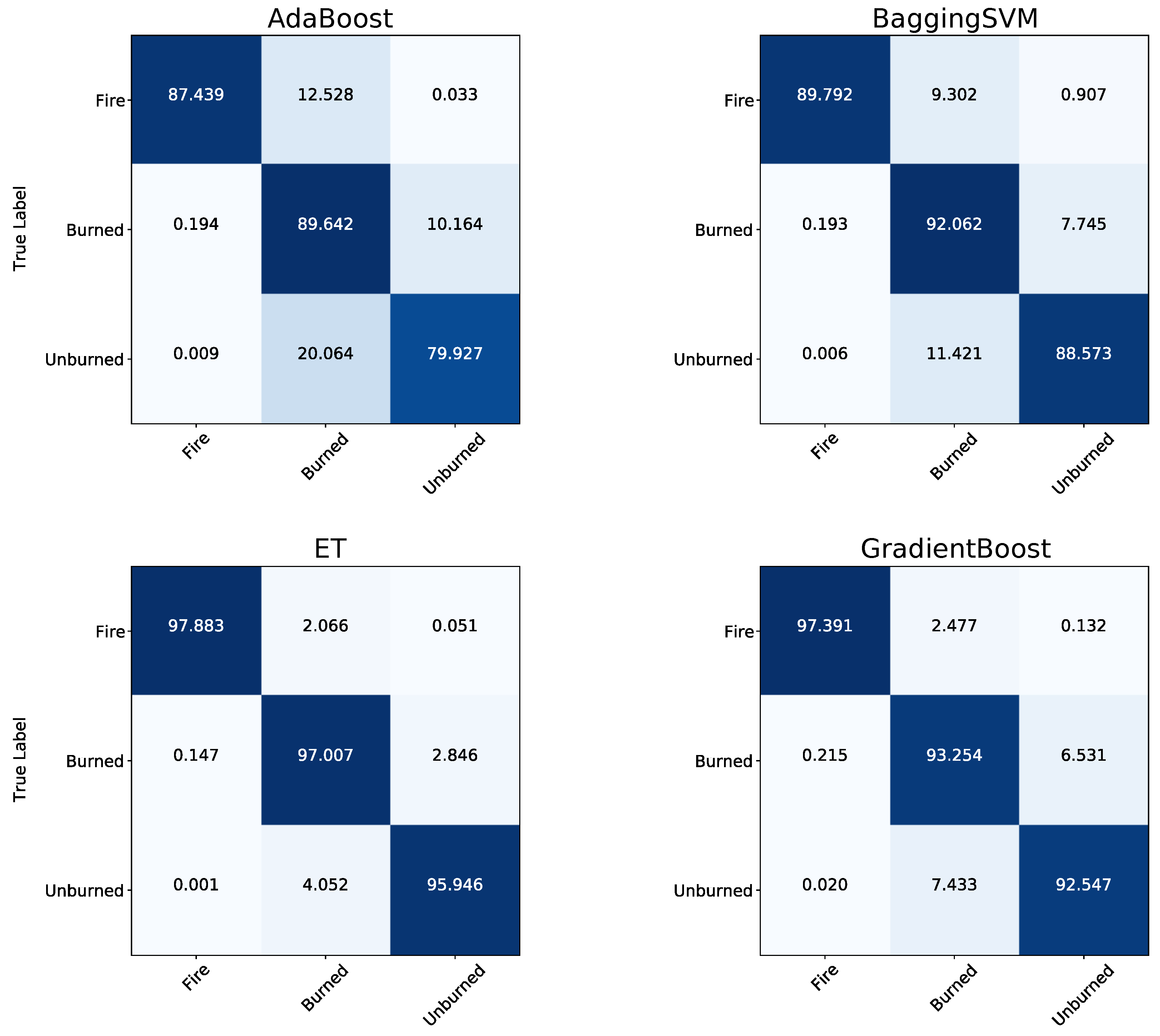
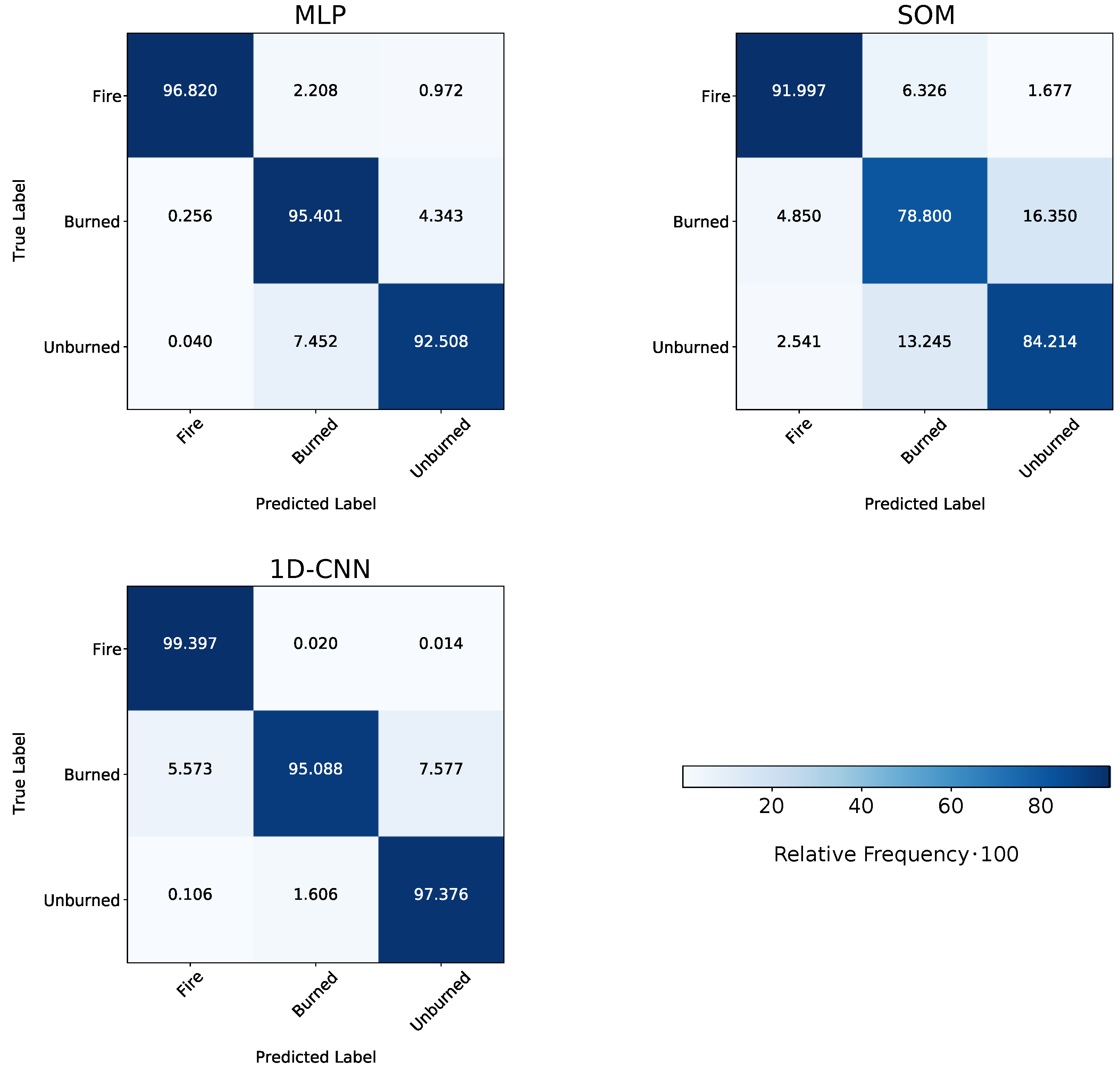
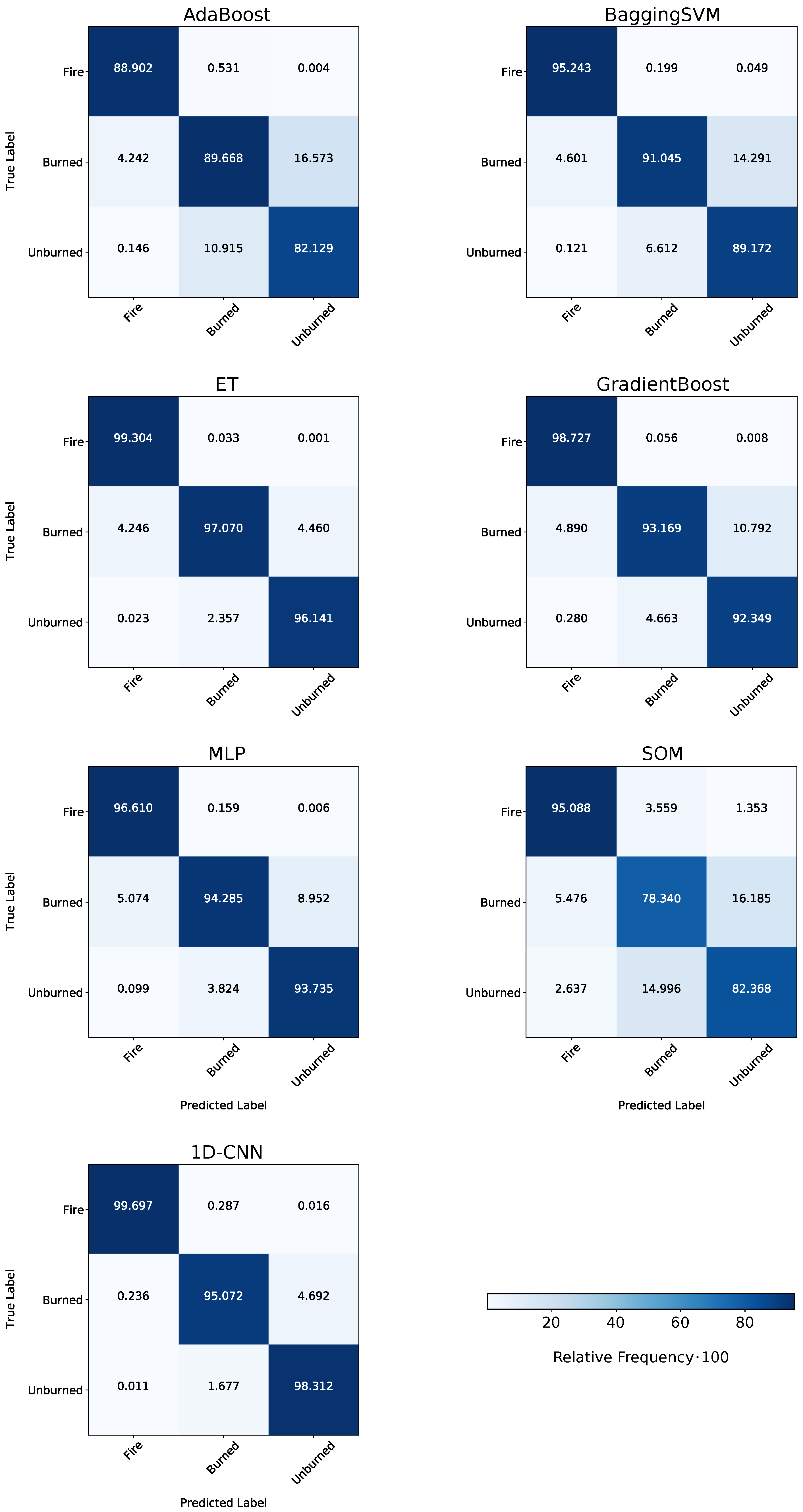
3.2. Classwise Performance of the Models
3.3. Classification Performances Concerning Different Subsets
3.4. Application of Two Selected Models on an Unknown Dataset and Their Performances
4. Discussion
4.1. Addressing the Challenge of Reference Data Generation for a Combined Detection
4.2. Separation of the Classes Regarding the Models’ Overall Classification Performance
4.3. Investigating the Classwise Separation on the Balanced Datasets
4.4. Evaluating the Classification Performances concerning Different Subsets
4.5. Investigating the Best Two Models’ Performances on an Unknown Dataset
5. Conclusions
Author Contributions
Funding
Acknowledgments
Conflicts of Interest
Appendix A. Distribution of the Data points after Undersampling
| Subsets | Total | Fire | Burned | Unburned |
|---|---|---|---|---|
| Train 1 | 1,707,832 | 79,859 | 1,010,220 | 617,753 |
| Uset 1 | 1,203,322 | 79,859 | 718,003 | 405,460 |
| Train 2 | 1,707,835 | 79,860 | 1,010,222 | 617,753 |
| Uset 2 | 1,203,327 | 79,860 | 718,006 | 405,461 |
| Train 3 | 1,707,842 | 79,857 | 1,010,227 | 617,758 |
| Uset 3 | 1,203,328 | 79,857 | 718,007 | 405,464 |
Appendix B. Hyperparameters
| Model | Package | Hyperparameter Setup |
|---|---|---|
| ET [72] | scikit-learn | |
| AdaBoost [73] | scikit-learn | |
| GradientBoost [74] | scikit-learn | |
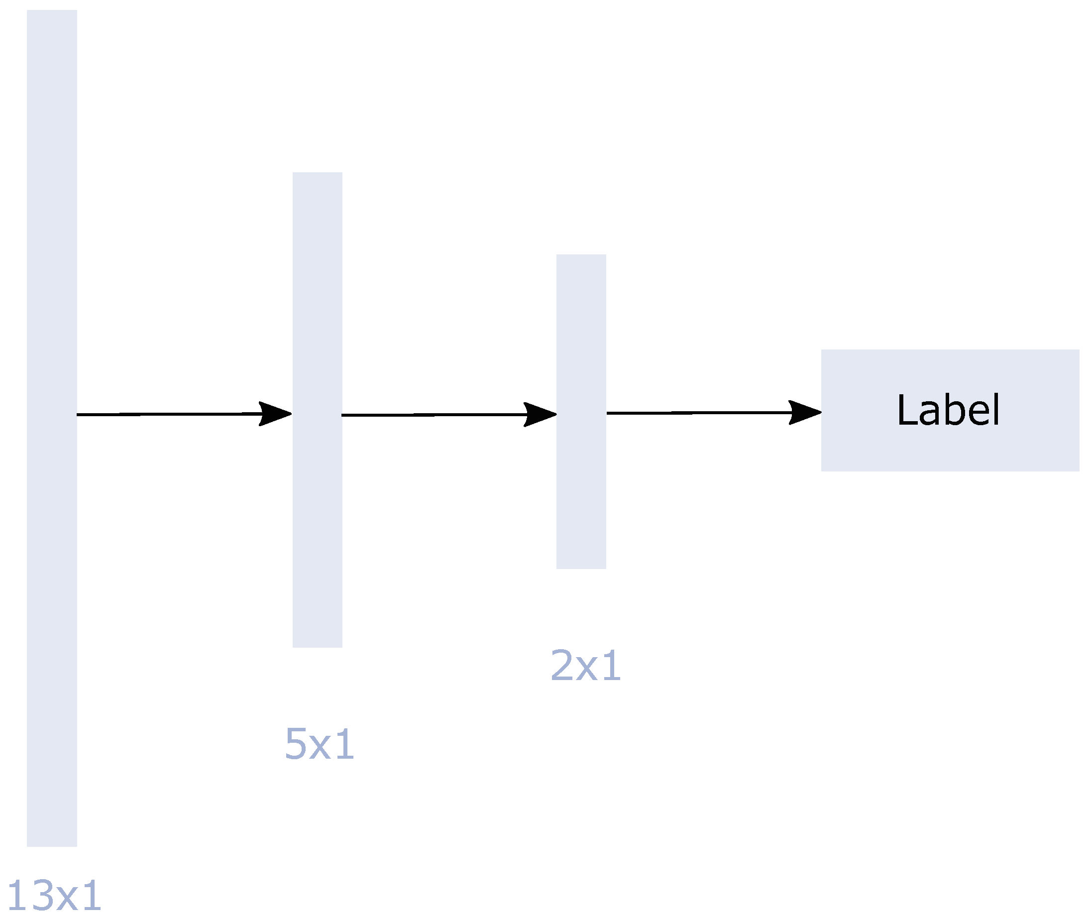
| MLP [75] | scikit-learn | |
| BaggingSVM [79] | scikit-learn | |
| SOM [63,77,78] | other | SOM size ; ; learning rates |
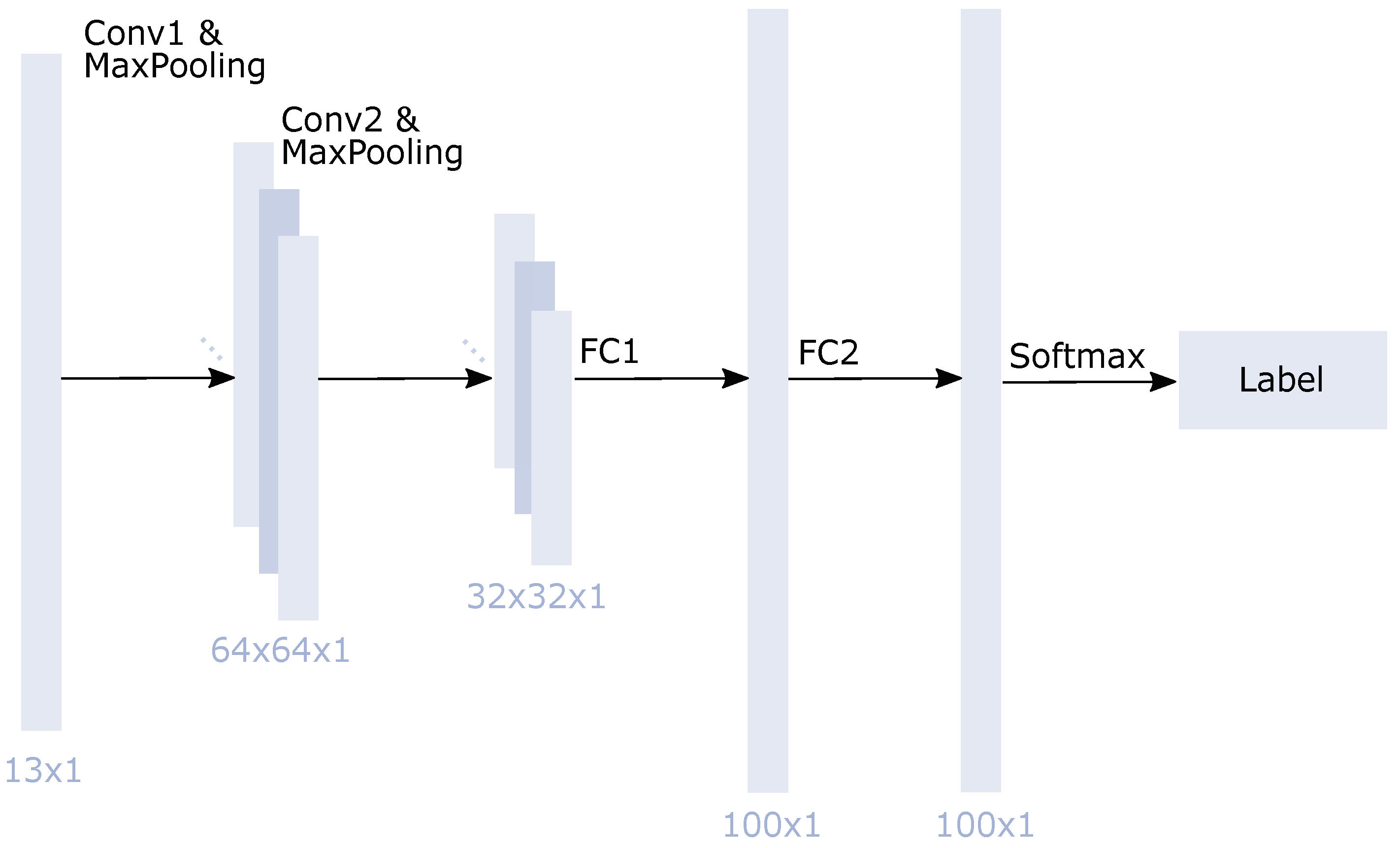
| 1D-CNN [80] | TensorFlow | Keras sequential model: ; 2 convolutional layers with ; 1 dense layer with 100 neurons; |
Appendix C. Performance on the Imbalanced Dataset
References
- Sharples, J.J.; Cary, G.J.; Fox-Hughes, P.; Mooney, S.; Evans, J.P.; Fletcher, M.S.; Fromm, M.; Grierson, P.F.; McRae, R.; Baker, P. Natural hazards in Australia: Extreme bushfire. Clim. Chang. 2016, 139, 85–99. [Google Scholar] [CrossRef]
- Boer, M.M.; de Dios, V.R.; Bradstock, R.A. Unprecedented burn area of Australian mega forest fires. Nat. Clim. Chang. 2020, 10, 171–172. [Google Scholar] [CrossRef]
- Lentile, L.B.; Holden, Z.A.; Smith, A.M.; Falkowski, M.J.; Hudak, A.T.; Morgan, P.; Lewis, S.A.; Gessler, P.E.; Benson, N.C. Remote sensing techniques to assess active fire characteristics and post-fire effects. Int. J. Wildland Fire 2006, 15, 319–345. [Google Scholar] [CrossRef]
- Bowman, D.M.; Balch, J.K.; Artaxo, P.; Bond, W.J.; Carlson, J.M.; Cochrane, M.A.; D’Antonio, C.M.; DeFries, R.S.; Doyle, J.C.; Harrison, S.P.; et al. Fire in the Earth system. Science 2009, 324, 481–484. [Google Scholar] [CrossRef] [PubMed]
- Filipponi, F. Exploitation of sentinel-2 time series to map burned areas at the national level: A case study on the 2017 Italy wildfires. Remote Sens. 2019, 11, 622. [Google Scholar] [CrossRef] [Green Version]
- Ghaffarian, S.; Kerle, N.; Pasolli, E.; Jokar Arsanjani, J. Post-disaster building database updating using automated deep learning: An integration of pre-disaster OpenStreetMap and multi-temporal satellite data. Remote Sens. 2019, 11, 2427. [Google Scholar] [CrossRef] [Green Version]
- Guth, J.; Wursthorn, S.; Braun, A.C.; Keller, S. Development of a generic concept to analyze the accessibility of emergency facilities in critical road infrastructure for disaster scenarios: Exemplary application for the 2017 wildfires in Chile and Portugal. Nat. Hazards 2019, 97, 979–999. [Google Scholar] [CrossRef]
- Henry, M.C.; Maingi, J.K.; McCarty, J. Fire on the Water Towers: Mapping Burn Scars on Mount Kenya Using Satellite Data to Reconstruct Recent Fire History. Remote Sens. 2019, 11, 104. [Google Scholar] [CrossRef] [Green Version]
- Guindos-Rojas, F.; Arbelo, M.; García-Lázaro, J.R.; Moreno-Ruiz, J.A.; Hernández-Leal, P.A. Evaluation of a Bayesian algorithm to detect Burned Areas in the Canary Islands’ Dry Woodlands and forests ecoregion using MODIS data. Remote Sens. 2018, 10, 789. [Google Scholar] [CrossRef] [Green Version]
- Schroeder, W.; Oliva, P.; Giglio, L.; Quayle, B.; Lorenz, E.; Morelli, F. Active fire detection using Landsat-8/OLI data. Remote Sens. Environ. 2016, 185, 210–220. [Google Scholar] [CrossRef] [Green Version]
- Giglio, L.; Csiszar, I.; Restás, Á.; Morisette, J.T.; Schroeder, W.; Morton, D.; Justice, C.O. Active fire detection and characterization with the advanced spaceborne thermal emission and reflection radiometer (ASTER). Remote Sens. Environ. 2008, 112, 3055–3063. [Google Scholar] [CrossRef]
- Crowley, M.A.; Cardille, J.A.; White, J.C.; Wulder, M.A. Multi-sensor, multi-scale, Bayesian data synthesis for mapping within-year wildfire progression. Remote Sens. Lett. 2019, 10, 302–311. [Google Scholar] [CrossRef]
- Chiaraviglio, N.; Artés, T.; Bocca, R.; López, J.; Gentile, A.; Ayanz, J.S.M.; Cortés, A.; Margalef, T. Automatic fire perimeter determination using MODIS hotspots information. In Proceedings of the 2016 IEEE 12th International Conference on e-Science (e-Science), Baltimore, MD, USA, 23–27 October 2016; pp. 414–423. [Google Scholar]
- Pereira, A.A.; Pereira, J.; Libonati, R.; Oom, D.; Setzer, A.W.; Morelli, F.; Machado-Silva, F.; De Carvalho, L.M.T. Burned area mapping in the Brazilian Savanna using a one-class support vector machine trained by active fires. Remote Sens. 2017, 9, 1161. [Google Scholar] [CrossRef] [Green Version]
- Cicala, L.; Angelino, C.V.; Fiscante, N.; Ullo, S.L. Landsat-8 and Sentinel-2 for fire monitoring at a local scale: A case study on Vesuvius. In Proceedings of the 2018 IEEE International Conference on Environmental Engineering (EE), Milan, Italy, 12–14 March 2018; pp. 1–6. [Google Scholar]
- Schroeder, W.; Oliva, P.; Giglio, L.; Csiszar, I.A. The New VIIRS 375 m active fire detection data product: Algorithm description and initial assessment. Remote Sens. Environ. 2014, 143, 85–96. [Google Scholar] [CrossRef]
- Gargiulo, M.; Dell’Aglio, D.A.G.; Iodice, A.; Riccio, D.; Ruello, G. A CNN-Based Super-Resolution Technique for Active Fire Detection on Sentinel-2 Data. In Proceedings of the 2019 PhotonIcs & Electromagnetics Research Symposium-Spring (PIERS-Spring), Rome, Italy, 17–20 June 2019; pp. 418–426. [Google Scholar]
- Oliva, P.; Schroeder, W. Assessment of VIIRS 375 m active fire detection product for direct burned area mapping. Remote Sens. Environ. 2015, 160, 144–155. [Google Scholar] [CrossRef]
- Stroppiana, D.; Pinnock, S.; Pereira, J.M.; Grégoire, J.M. Radiometric analysis of SPOT-VEGETATION images for burnt area detection in Northern Australia. Remote Sens. Environ. 2002, 82, 21–37. [Google Scholar] [CrossRef]
- Thomas, P.J.; Hersom, C.H.; Kourtz, P.; Buttner, G.J. Space-based forest fire detection concept. In Infrared Spaceborne Remote Sensing III; International Society for Optics and Photonics: Bellingham, WA, USA, 1995; Volume 2553, pp. 104–115. [Google Scholar]
- Giglio, L.; Descloitres, J.; Justice, C.O.; Kaufman, Y.J. An enhanced contextual fire detection algorithm for MODIS. Remote Sens. Environ. 2003, 87, 273–282. [Google Scholar] [CrossRef]
- NASA. MODIS Specifications; NASA: Washington, DC, USA, 2021. [Google Scholar]
- Kumar, S.S.; Roy, D.P. Global operational land imager Landsat-8 reflectance-based active fire detection algorithm. Int. J. Digit. Earth 2018, 11, 154–178. [Google Scholar] [CrossRef] [Green Version]
- Schroeder, W.; Prins, E.; Giglio, L.; Csiszar, I.; Schmidt, C.; Morisette, J.; Morton, D. Validation of GOES and MODIS active fire detection products using ASTER and ETM+ data. Remote Sens. Environ. 2008, 112, 2711–2726. [Google Scholar] [CrossRef]
- Engelbrecht, J.; Theron, A.; Vhengani, L.; Kemp, J. A simple normalized difference approach to burnt area mapping using multi-polarisation C-Band SAR. Remote Sens. 2017, 9, 764. [Google Scholar] [CrossRef] [Green Version]
- Siegert, F.; Hoffmann, A.A. The 1998 forest fires in East Kalimantan (Indonesia): A quantitative evaluation using high resolution, multitemporal ERS-2 SAR images and NOAA-AVHRR hotspot data. Remote Sens. Environ. 2000, 72, 64–77. [Google Scholar] [CrossRef]
- Axel, A.C. Burned area mapping of an escaped fire into tropical dry forest in Western Madagascar using multi-season Landsat OLI Data. Remote Sens. 2018, 10, 371. [Google Scholar] [CrossRef] [Green Version]
- Polychronaki, A.; Gitas, I.Z. The development of an operational procedure for burned-area mapping using object-based classification and ASTER imagery. Int. J. Remote Sens. 2010, 31, 1113–1120. [Google Scholar] [CrossRef]
- Gitas, I.Z.; Mitri, G.H.; Ventura, G. Object-based image classification for burned area mapping of Creus Cape, Spain, using NOAA-AVHRR imagery. Remote Sens. Environ. 2004, 92, 409–413. [Google Scholar] [CrossRef]
- Grivei, A.C.; Văduva, C.; Datcu, M. Assessment of Burned Area Mapping Methods for Smoke Covered Sentinel-2 Data. In Proceedings of the 2020 13th International Conference on Communications (COMM), Bucharest, Romania, 18–20 June 2020; pp. 189–192. [Google Scholar]
- Knopp, L.; Wieland, M.; Rättich, M.; Martinis, S. A Deep Learning Approach for Burned Area Segmentation with Sentinel-2 Data. Remote Sens. 2020, 12, 2422. [Google Scholar] [CrossRef]
- Rashkovetsky, D.; Mauracher, F.; Langer, M.; Schmitt, M. Wildfire Detection from Multi-sensor Satellite Imagery Using Deep Semantic Segmentation. IEEE J. Sel. Top. Appl. Earth Obs. Remote Sens. 2021, 14, 7001–7016. [Google Scholar] [CrossRef]
- Rauste, Y.; Herland, E.; Frelander, H.; Soini, K.; Kuoremaki, T.; Ruokari, A. Satellite-based forest fire detection for fire control in boreal forests. Int. J. Remote Sens. 1997, 18, 2641–2656. [Google Scholar] [CrossRef]
- Matson, M.; Stephens, G.; Robinson, J. Fire detection using data from the NOAA-N satellites. Int. J. Remote Sens. 1987, 8, 961–970. [Google Scholar] [CrossRef]
- Xie, Z.; Song, W.; Ba, R.; Li, X.; Xia, L. A spatiotemporal contextual model for forest fire detection using Himawari-8 satellite data. Remote Sens. 2018, 10, 1992. [Google Scholar] [CrossRef] [Green Version]
- Flasse, S.; Ceccato, P. A contextual algorithm for AVHRR fire detection. Int. J. Remote Sens. 1996, 17, 419–424. [Google Scholar] [CrossRef]
- Giglio, L.; Schroeder, W.; Justice, C.O. The collection 6 MODIS active fire detection algorithm and fire products. Remote Sens. Environ. 2016, 178, 31–41. [Google Scholar] [CrossRef] [PubMed] [Green Version]
- Di Biase, V.; Laneve, G. Geostationary sensor based forest fire detection and monitoring: An improved version of the SFIDE algorithm. Remote Sens. 2018, 10, 741. [Google Scholar] [CrossRef] [Green Version]
- San-Miguel-Ayanz, J.; Ravail, N. Active fire detection for fire emergency management: Potential and limitations for the operational use of remote sensing. Nat. Hazards 2005, 35, 361–376. [Google Scholar] [CrossRef] [Green Version]
- Koltunov, A.; Ustin, S.L.; Quayle, B.; Schwind, B.; Ambrosia, V.G.; Li, W. The development and first validation of the GOES Early Fire Detection (GOES-EFD) algorithm. Remote Sens. Environ. 2016, 184, 436–453. [Google Scholar] [CrossRef] [Green Version]
- Kurum, M. C-band SAR backscatter evaluation of 2008 Gallipoli forest fire. IEEE Geosci. Remote Sens. Lett. 2015, 12, 1091–1095. [Google Scholar] [CrossRef]
- Ruecker, G.; Siegert, F. Burn scar mapping and fire damage assessment using ERS-2 Sar images in East Kalimantan, Indonesia. Int. Arch. Photogramm. Remote Sens. 2000, 33, 1286–1293. [Google Scholar]
- Goodenough, D.G.; Chen, H.; Richardson, A.; Cloude, S.; Hong, W.; Li, Y. Mapping fire scars using Radarsat-2 polarimetric SAR data. Can. J. Remote Sens. 2011, 37, 500–509. [Google Scholar] [CrossRef] [Green Version]
- Wei, J.; Zhang, Y.; Wu, H.; Cui, B. The Automatic Detection of Fire Scar in Alaska using Multi-Temporal PALSAR Polarimetric SAR Data. Can. J. Remote Sens. 2018, 44, 447–461. [Google Scholar] [CrossRef]
- Ban, Y.; Zhang, P.; Nascetti, A.; Bevington, A.R.; Wulder, M.A. Near real-time wildfire progression monitoring with Sentinel-1 SAR time series and deep learning. Sci. Rep. 2020, 10, 1–15. [Google Scholar] [CrossRef] [Green Version]
- Mithal, V.; Nayak, G.; Khandelwal, A.; Kumar, V.; Nemani, R.; Oza, N.C. Mapping burned areas in tropical forests using a novel machine learning framework. Remote Sens. 2018, 10, 69. [Google Scholar] [CrossRef] [Green Version]
- Libonati, R.; DaCamara, C.C.; Setzer, A.W.; Morelli, F.; Melchiori, A.E. An algorithm for burned area detection in the Brazilian Cerrado using 4 μm MODIS imagery. Remote Rens. 2015, 7, 15782–15803. [Google Scholar]
- Bastarrika, A.; Alvarado, M.; Artano, K.; Martinez, M.P.; Mesanza, A.; Torre, L.; Ramo, R.; Chuvieco, E. BAMS: A tool for supervised burned area mapping using Landsat data. Remote Sens. 2014, 6, 12360–12380. [Google Scholar] [CrossRef] [Green Version]
- Stroppiana, D.; Bordogna, G.; Carrara, P.; Boschetti, M.; Boschetti, L.; Brivio, P.A. A method for extracting burned areas from Landsat TM/ETM+ images by soft aggregation of multiple Spectral Indices and a region growing algorithm. ISPRS J. Photogramm. Remote Sens. 2012, 69, 88–102. [Google Scholar] [CrossRef]
- Kurnaz, B.; Bayik, C.; Abdikan, S. Forest Fire Area Detection by Using Landsat-8 and Sentinel-2 Satellite Images: A Case Study in Mugla, Turkey; Research Square: Ankara, Turkey, 2020. [Google Scholar]
- Bastarrika, A.; Chuvieco, E.; Martin, P.M. Mapping burned areas from Landsat TM/ETM+ data with a two-phase algorithm: Balancing omission and commission errors. Remote Sens. Environ. 2011, 115, 1003–1012. [Google Scholar] [CrossRef]
- Bastarrika, A.; Barrett, B.; Roteta, E.; Akizu, O.; Mesanza, A.; Torre, L.; Anaya, J.A.; Rodriguez-Montellano, A.; Chuvieco, E. Mapping burned areas in Latin America from Landsat-8 with Google Earth Engine. Remote Sens. 2018. [Google Scholar] [CrossRef]
- Ramo, R.; Chuvieco, E. Developing a random forest algorithm for MODIS global burned area classification. Remote Sens. 2017, 9, 1193. [Google Scholar] [CrossRef] [Green Version]
- Mitri, G.H.; Gitas, I.Z. The development of an object-oriented classification model for operational burned area mapping on the Mediterranean island of Thasos using LANDSAT TM images. In Forest Fire Research & Wildland Fire Safety; Millpress: Bethlehem, PA, USA, 2002; pp. 1–12. [Google Scholar]
- Çömert, R.; Matci, D.K.; Avdan, U. Object Based Burned Area Mapping with Random Forest Algorithm. Int. J. Eng. Geosci. 2019, 4, 78–87. [Google Scholar] [CrossRef]
- Mallinis, G.; Koutsias, N. Comparing ten classification methods for burned area mapping in a Mediterranean environment using Landsat TM satellite data. Int. J. Remote Sens. 2012, 33, 4408–4433. [Google Scholar] [CrossRef]
- Pereira, M.C.; Setzer, A.W. Spectral characteristics of fire scars in Landsat-5 TM images of Amazonia. Remote Sens. 1993, 14, 2061–2078. [Google Scholar] [CrossRef]
- Mitrakis, N.E.; Mallinis, G.; Koutsias, N.; Theocharis, J.B. Burned area mapping in Mediterranean environment using medium-resolution multi-spectral data and a neuro-fuzzy classifier. Int. J. Image Data Fusion 2012, 3, 299–318. [Google Scholar] [CrossRef]
- Brand, A.; Manandhar, A. Semantic Segmentation of Burned Areas in Satellite Images Using a U-Net Convolutional Neural Network. ISPRS-Int. Arch. Photogramm. Remote Sens. Spat. Inf. Sci. 2021, 43, 47–53. [Google Scholar] [CrossRef]
- Barducci, A.; Guzzi, D.; Marcoionni, P.; Pippi, I. Infrared detection of active fires and burnt areas: Theory and observations. Infrared Phys. Technol. 2002, 43, 119–125. [Google Scholar] [CrossRef]
- Calle, A.; Casanova, J.; Romo, A. Fire detection and monitoring using MSG Spinning Enhanced Visible and Infrared Imager (SEVIRI) data. J. Geophys. Res. Biogeosci. 2006, 111. [Google Scholar] [CrossRef]
- Michael, Y.; Lensky, I.M.; Brenner, S.; Tchetchik, A.; Tessler, N.; Helman, D. Economic assessment of fire damage to urban forest in the wildland–urban interface using planet satellites constellation images. Remote Sens. 2018, 10, 1479. [Google Scholar] [CrossRef] [Green Version]
- Riese, F.M.; Keller, S. Supervised, Semi-Supervised, and Unsupervised Learning for Hyperspectral Regression. In Hyperspectral Image Analysis; Springer: Cham, Switzerland, 2020; pp. 187–232. [Google Scholar]
- State of California CAL FIRE. Available online: https://frap.fire.ca.gov/mapping/gis-data/ (accessed on 13 January 2022).
- Buchhorn, M.; Lesiv, M.; Tsendbazar, N.E.; Herold, M.; Bertels, L.; Smets, B. Copernicus Global Land Cover Layers—Collection 2. Remote Sens. 2020, 12, 1044. [Google Scholar] [CrossRef] [Green Version]
- Wu, Q. geemap: A Python package for interactive mapping with Google Earth Engine. J. Open Source Softw. 2020, 5, 2305. [Google Scholar] [CrossRef]
- Weiss, G.M. Foundations of imbalanced learning. In Imbalanced Learning: Foundations, Algorithms, and Applications; Wiley: Hoboken, NJ, USA, 2013; pp. 13–41. [Google Scholar]
- Chawla, N.V.; Japkowicz, N.; Kotcz, A. Special issue on learning from imbalanced data sets. ACM SIGKDD Explor. Newsl. 2004, 6, 1–6. [Google Scholar] [CrossRef]
- Liu, X.Y.; Wu, J.; Zhou, Z.H. Exploratory undersampling for class-imbalance learning. IEEE Trans. Syst. Man Cybern. Part B Cybern. 2008, 39, 539–550. [Google Scholar]
- Kattenborn, T.; Leitloff, J.; Schiefer, F.; Hinz, S. Review on Convolutional Neural Networks (CNN) in vegetation remote sensing. ISPRS J. Photogramm. Remote Sens. 2021, 173, 24–49. [Google Scholar] [CrossRef]
- Drummond, C.; Holte, R.C. C4. 5, class imbalance, and cost sensitivity: Why under-sampling beats over-sampling. In Workshop on Learning from Imbalanced Datasets II; Citeseer: Princeton, NJ, USA, 2003; Volume 11, pp. 1–8. [Google Scholar]
- Geurts, P.; Ernst, D.; Wehenkel, L. Extremely randomized trees. Mach. Learn. 2006, 63, 3–42. [Google Scholar] [CrossRef] [Green Version]
- Freund, Y.; Schapire, R.E. A decision-theoretic generalization of on-line learning and an application to boosting. J. Comput. Syst. Sci. 1997, 55, 119–139. [Google Scholar] [CrossRef] [Green Version]
- Friedman, J.H. Greedy function approximation: A gradient boosting machine. In Annals of Statistics; Institute of Mathematical Statistics: Shaker Heights, OH, USA, 2001; pp. 1189–1232. [Google Scholar]
- Hinton, G.E. Connectionist learning procedures. In Machine Learning; Elsevier: Amsterdam, The Netherlands, 1990; pp. 555–610. [Google Scholar]
- Riese, F.M.; Keller, S.; Hinz, S. Supervised and semi-supervised self-organizing maps for regression and classification focusing on hyperspectral data. Remote Sens. 2020, 12, 7. [Google Scholar] [CrossRef] [Green Version]
- Riese, F.M.; Keller, S. Introducing a framework of self-organizing maps for regression of soil moisture with hyperspectral data. In Proceedings of the IGARSS 2018-2018 IEEE International Geoscience and Remote Sensing Symposium, Valencia, Spain, 22–27 July 2018; pp. 6151–6154. [Google Scholar]
- Kohonen, T. The self-organizing map. Proc. IEEE 1990, 78, 1464–1480. [Google Scholar] [CrossRef]
- Kim, H.C.; Pang, S.; Je, H.M.; Kim, D.; Bang, S.Y. Support vector machine ensemble with bagging. In International Workshop on Support Vector Machines; Springer: Berlin, Germany, 2002; pp. 397–408. [Google Scholar]
- Riese, F.M.; Keller, S. Soil texture classification with 1D convolutional neural networks based on hyperspectral data. ISPRS Ann. Photogramm. Remote Sens. Spat. Inf. Sci. 2019, IV-2/W5, 615–621. [Google Scholar] [CrossRef] [Green Version]
- Hansen, M.C.; DeFries, R.S.; Townshend, J.R.; Sohlberg, R. Global land cover classification at 1 km spatial resolution using a classification tree approach. Int. J. Remote Sens. 2000, 21, 1331–1364. [Google Scholar] [CrossRef]
- Lasaponara, R.; Proto, M.; Aromando, A.; Cardettini, G.; Varela, V.; Danese, M. On the mapping of burned areas and burn severity using self organizing map and sentinel-2 data. IEEE Geosci. Remote Sens. Lett. 2019, 17, 854–858. [Google Scholar] [CrossRef]
- Riese, F.M. SuSi: Supervised Self-Organizing Maps in Python; Zenodo: Geneve, Switzerland, 2019. [Google Scholar] [CrossRef]
- Pedregosa, F.; Varoquaux, G.; Gramfort, A.; Michel, V.; Thirion, B.; Grisel, O.; Blondel, M.; Prettenhofer, P.; Weiss, R.; Dubourg, V.; et al. Scikit-learn: Machine Learning in Python. J. Mach. Learn. Res. 2011, 12, 2825–2830. [Google Scholar]
- Rosenblatt, F. The perceptron: A probabilistic model for information storage and organization in the brain. Psychol. Rev. 1958, 65, 386. [Google Scholar] [CrossRef] [Green Version]
- Liu, L.; Ji, M.; Buchroithner, M. Transfer learning for soil spectroscopy based on convolutional neural networks and its application in soil clay content mapping using hyperspectral imagery. Sensors 2018, 18, 3169. [Google Scholar] [CrossRef] [Green Version]
- Hu, W.; Huang, Y.; Wei, L.; Zhang, F.; Li, H. Deep convolutional neural networks for hyperspectral image classification. J. Sens. 2015, 2015, 258619. [Google Scholar] [CrossRef] [Green Version]
- Li, L.; Jamieson, K.; DeSalvo, G.; Rostamizadeh, A.; Talwalkar, A. Hyperband: A novel bandit-based approach to hyperparameter optimization. J. Mach. Learn. Res. 2017, 18, 6765–6816. [Google Scholar]
- Mosley, L. A Balanced Approach to the Multi-Class Imbalance Problem; Iowa State University: Ames, IA, USA, 2013. [Google Scholar]
- Cervone, G.; Sava, E.; Huang, Q.; Schnebele, E.; Harrison, J.; Waters, N. Using Twitter for tasking remote-sensing data collection and damage assessment: 2013 Boulder flood case study. Int. J. Remote Sens. 2016, 37, 100–124. [Google Scholar] [CrossRef]
- Bruneau, P.; Brangbour, E.; Marchand-Maillet, S.; Hostache, R.; Chini, M.; Pelich, R.M.; Matgen, P.; Tamisier, T. Measuring the Impact of Natural Hazards with Citizen Science: The Case of Flooded Area Estimation Using Twitter. Remote Sens. 2021, 13, 1153. [Google Scholar] [CrossRef]
- Kruspe, A.; Häberle, M.; Hoffmann, E.J.; Rode-Hasinger, S.; Abdulahhad, K.; Zhu, X.X. Changes in Twitter geolocations: Insights and suggestions for future usage. arXiv 2021, arXiv:2108.12251. [Google Scholar]
- Abadi, M.; Barham, P.; Chen, J.; Chen, Z.; Davis, A.; Dean, J.; Devin, M.; Ghemawat, S.; Irving, G.; Isard, M.; et al. Tensorflow: A system for large-scale machine learning. In Proceedings of the 12th Symposium on Operating Systems Design and Implementation, Savannah, GA, USA, 2–4 November 2016; pp. 265–283. [Google Scholar]

| Test I: S1 T | Test II: Subset 2 | Test II: Subset 3 | Test III: Spain 1 |
|---|---|---|---|
| 569,277 | 2,846,391 | 2,846,403 | 213,120 |
| Model | OA | Kappa | F1 | Prec | AA | BA |
|---|---|---|---|---|---|---|
| AdaBoost | 91.2 | 73.6 | 86.8 | 86.8 | 86.9 | 86.9 |
| BaggingSVM | 93.7 | 81.1 | 90.5 | 90.6 | 90.5 | 91.8 |
| ET | 97.9 | 93.6 | 96.8 | 96.8 | 96.3 | 97.5 |
| GradientBoost | 95.3 | 86.2 | 93.0 | 93.1 | 93.0 | 94.7 |
| MLP | 96.1 | 88.4 | 94.2 | 94.2 | 94.2 | 94.9 |
| SOM | 86.9 | 63.0 | 81.0 | 82.8 | 80.3 | 85.3 |
| 1D-CNN | 97.6 | 92.9 | 96.4 | 96.5 | 96.4 | 97.7 |
| Model | Training | Uset 1 | Uset 2 | Uset 3 | |||
|---|---|---|---|---|---|---|---|
| Test | Subset 2 | Subset 3 | Subset 1 | Subset 3 | Subset 1 | Subset 2 | |
| AdaBoost | 85.6 | 85.6 | 86.5 | 86.5 | 86.9 | 86.9 | |
| ET | 96.6 | 96.6 | 97.5 | 96.7 | 97.5 | 96.7 | |
| GradientBoost | 93.0 | 93.0 | 93.1 | 93.1 | 93.0 | 93.0 | |
| MLP | 94.0 | 94.0 | 94.0 | 94.0 | 94.1 | 94.2 | |
| Model | OA | Kappa | F1 | Prec | AA | BA |
|---|---|---|---|---|---|---|
| ET | 99.6 | 79.1 | 93.7 | 94.3 | 93.4 | 82.3 |
| 1D-CNN | 99.8 | 83.2 | 95.0 | 95.4 | 94.9 | 91.0 |
Publisher’s Note: MDPI stays neutral with regard to jurisdictional claims in published maps and institutional affiliations. |
© 2022 by the authors. Licensee MDPI, Basel, Switzerland. This article is an open access article distributed under the terms and conditions of the Creative Commons Attribution (CC BY) license (https://creativecommons.org/licenses/by/4.0/).
Share and Cite
Florath, J.; Keller, S. Supervised Machine Learning Approaches on Multispectral Remote Sensing Data for a Combined Detection of Fire and Burned Area. Remote Sens. 2022, 14, 657. https://doi.org/10.3390/rs14030657
Florath J, Keller S. Supervised Machine Learning Approaches on Multispectral Remote Sensing Data for a Combined Detection of Fire and Burned Area. Remote Sensing. 2022; 14(3):657. https://doi.org/10.3390/rs14030657
Chicago/Turabian StyleFlorath, Janine, and Sina Keller. 2022. "Supervised Machine Learning Approaches on Multispectral Remote Sensing Data for a Combined Detection of Fire and Burned Area" Remote Sensing 14, no. 3: 657. https://doi.org/10.3390/rs14030657
APA StyleFlorath, J., & Keller, S. (2022). Supervised Machine Learning Approaches on Multispectral Remote Sensing Data for a Combined Detection of Fire and Burned Area. Remote Sensing, 14(3), 657. https://doi.org/10.3390/rs14030657