Abstract
Bushfires pose a severe risk, among others, to humans, wildlife, and infrastructures. Rapid detection of fires is crucial for fire-extinguishing activities and rescue missions. Besides, mapping burned areas also supports evacuation and accessibility to emergency facilities. In this study, we propose a generic approach for detecting fires and burned areas based on machine learning (ML) approaches and remote sensing data. While most studies investigated either the detection of fires or mapping burned areas, we addressed and evaluated, in particular, the combined detection on three selected case study regions. Multispectral Sentinel-2 images represent the input data for the supervised ML models. First, we generated the reference data for the three target classes, burned, unburned, and fire, since no reference data were available. Second, the three regional fire datasets were preprocessed and divided into training, validation, and test subsets according to a defined schema. Furthermore, an undersampling approach ensured the balancing of the datasets. Third, seven selected supervised classification approaches were used and evaluated, including tree-based models, a self-organizing map, an artificial neural network, and a one-dimensional convolutional neural network (1D-CNN). All selected ML approaches achieved satisfying classification results. Moreover, they performed a highly accurate fire detection, while separating burned and unburned areas was slightly more challenging. The 1D-CNN and extremely randomized tree were the best-performing models with an overall accuracy score of 98% on the test subsets. Even on an unknown test dataset, the 1D-CNN achieved high classification accuracies. This generalization is even more valuable for any use-case scenario, including the organization of fire-fighting activities or civil protection. The proposed combined detection could be extended and enhanced with crowdsourced data in further studies.
1. Introduction
In recent years, large-scale bushfires have tended to occur more frequently [1]. The most recent, large-scale, and heavily media-covered fire event occurred in the 2019/2020 bushfire season in south-eastern Australia. These fires burned several million hectares of land [2]. Bushfires affect the ecological, social, and economic environment significantly [3,4]. Detecting active fires quickly and on a larger scale is a critical task in the context of natural hazard management. Reliable and rapid detection of fires, for example, improves the coordination of fire-extinguishing activities and rescue missions.
Although burned area detection is not directly linked to immediate life-saving activities, mapping such burned areas supports a long-term evaluation of ecological and economic damages [5,6]. Burned areas often remain impassable for traffic or rescue vehicles [7] and threaten inhabitants several days after the actual fire has passed.
Most studies have not considered the distinction between burned areas and areas covered with actual bushfires, but focused on the detection and mapping of either one of them (burned area [8,9]; active fire [10,11]). In some studies, areas with active fires and burned areas were declared as one single class compared to the class Unburned [12,13].
In contrast, we attached importance to this distinction between burned areas and areas covered with actual fires. The main reason for this clear distinction is that either of the characteristics poses different challenges concerning risk management or rescue mission planning. In addition, when investigating the accessibility of road networks during and after bushfires, the information about whether an area is burned or contains fires constitutes an essential factor. While roads within a fire area are impassable, roads within a burned area might be usable to a certain degree. A Burned area is referred to as an area that happens to be a place of a bushfire a short time ago. A short time ago means, in this context, several days after the first detected fire ended and its influence on the landscape is still apparent [14]. An area with Fire means a burning fire is present, which can be either the main fire front or even a small area of smoldering brushwood [11].
The detection of fire and burned area can be achieved with remote sensing data, as we observed an increasing availability of these data in recent years. Many different approaches have already been applied for either active fire detection (mostly rule-based approaches) or burned area mapping (data-driven or rule-based approaches). In this study, we wanted to concentrate on investigating and evaluating several different machine learning (ML) approaches for a combined fire and burned area detection. The task of detecting active fires and burned areas based on ML approaches with remote sensing data includes several challenges. In the following, we briefly describe the main challenges that we addressed:
- Combined detection of active fire and burned area: We focused on detecting active fires and burned areas in one, combined data-driven approach. In existing studies, different approaches have been used for the two sub-tasks [15], if a distinction was performed between burned area and active fire. We developed a methodology to detect active fires and burned areas in one go using the same ML approach for both sub-tasks;
- Configuration of a generic concept: The concept is setup to enable a generic detection of fire areas and burned areas. Thus, we can distinguish fire and burned area incidents worldwide on an appropriate scale with the given methodological approach independently of prior or detailed knowledge of the appearance of either class in the investigated region. This novel workflow enables facile detection of both relevant areas in one go, which can be used for further risk management or other applications;
- Selection of appropriate ML approaches: Many ML approaches would be eligible to carry out the task of fire and burned area detection. We investigated and evaluated the applicability of several ML approaches and selected the best-performing for a possible application;
- Generation of reference data: Reference data are required for the training and testing steps of ML approaches. Since appropriate reference data were not available for active fires nor burned areas, large-scale reference data were generated. This generation was also set up as a generic concept that can be used for reference data manufacturing in any fire and burned area detection application worldwide;
- Detection at a high spatial resolution: For subsequent risk analysis, fire and burned area detection needs to be possible with very high accuracy, requiring a high spatial resolution of the chosen satellite data. Several types of remote sensing data can be used, but we relied on optical remote sensing data since they generally provide a higher spatial resolutions than, for example, thermal data [16]. The analysis was accomplished with the use of Sentinel-2 data, which provide a spatial resolution of 10 m in several bands [15]. With a spatial resolution of 10 m, we can ensure a much more accurate prediction of fires and burned areas affecting structures (such as roads) in these small dimensions.
Section 1.1 gives a short overview of related studies that address fire or burned area detection and propose several different supervised learning approaches for this purpose. We briefly describe the study area, the data basis, and the ML methodology in Section 2. The results (Section 3) of the data derivation and the classification are explained, followed by an application of the generated workflow on an independent, unseen area. Finally, we discuss the results (Section 4) and conclude the study with a resume (Section 5).
1.1. Research Background
Currently, existing studies cover either the topic of active fire detection or burned area mapping (see, for example, [16,17,18]). Therefore, we structured the related work into two parts: an overview of studies dealing with active fire detection and studies dealing with burned area mapping. A variety of remote sensing techniques have been used for both topics. First, the remote sensing data differ, covering different spectral wavelengths. Second, the applied approaches vary, although relying on the same remote sensing data. For both tasks, we describe the data used in different studies, on the one hand, and the methodological approaches to evaluate these data, on the other. Table 1, Table 2 and Table 3 summarize the related studies. We organized the studies according to the instruments used for recording reflection in different band lengths within different sections of the electromagnetic spectrum. Bands in certain electromagnetic spectrum sections were used in the analysis of the respective studies, while other bands provided by the same mission instrument were not used in some cases. This overlap may lead to sensors, e.g., the Moderate Resolution Imaging Spectroradiometer (MODIS), being named in the Thermal and Optical categories in our overview.
Fire detection and burned area detection rely on different principles, since the spectral reflectance differs in all sections of the electromagnetic spectrum for the two tasks. Therefore, the data used vary between the tasks. While thermal data are an obvious choice for fire detection (see Table 1), they are not helpful for burned areas after cooling down. In the case of burned area mapping, change detection approaches are more commonly applied. Change detection can be carried out using several different data such as Synthetic Aperture Radar (SAR) or optical data such as the Satellite Pour l’Observation de la Terre (SPOT; Satellite for Observation of Earth) [19] satellite.
When focusing on active fire detection, longwave thermal sensors are the most widespread data source [16,20,21]. Commonly used sensors are MODIS, the Visible Infrared Imaging Radiometer Suite (VIIRS), the Advanced Very High Resolution Radiometer (AVHHR), the Geostationary Operational Environmental Satellite (GOES), the Spinning Enhanced Visible and InfraRed Imager (SEVIRI), and others (see Table 1). While the approach with thermal data is relatively slightly susceptible to errors due to the nature of the fire, most sensors providing thermal data have a low resolution. Examples are the MODIS and VIIRS sensors with spatial resolutions of 250 m–1000 m [22] and 375 m–750 m, respectively. A higher resolution is offered by optical multispectral sensor data. In this category, the Landsat sensor is exploited for the task of fire detection [10,23]. The Advanced Spaceborne Thermal Emission and Reflection Radiometer (ASTER) sensor’s short-wave infrared (SWIR) bands [24], as well as its thermal bands [11] are used for fire detection.
For mapping burned areas, an even wider variety of different data is used (see Table 2). Several studies relied on SAR data such as Radarsat-2 [25], Sentinel-1 [25], and European Remote Sensing (ERS)-2 [26]. For the task of near-real-time burned area detection, as in our case, SAR data cannot be used, since satellite images from before the outbreak are necessary to differentiate between several time steps. To facilitate the detection of burned areas near real time, the detection with data in the optical spectrum is applied. Data in the visible, near-infrared (NIR), and SWIR spectrum, such as Landsat [8,27], ASTER [28], the Project for On-Board Autonomy-Vegetation (Proba-V) [14], and the National Oceanic and Atmospheric Administration (NOAA) [29] satellites, have been used. Some of the studies relied on Sentinel-2 data [5,25,30,31]. Just as for burned area detection, thermal sensor data are also used for active fire detection. MODIS data [9] and VIIRS data [18] are commonly used, while some studies used data from a combination of different sensors, such as Henry et al. [8] (MODIS and Landsat), Crowley et al. [12] (MODIS, Landsat, and Sentinel), or Rashkovetsky et al. [32] (Sentinel-1/Sentinel-2/Sentinel-3/MODIS).

Table 1.
Overview of the related work concerning fire detection. The following abbreviations are used: ASTER—Advanced Spaceborne Thermal Emission and Reflection Radiometer; AVHHR—Advanced Very High Resolution Radiometer; NOAA—National Oceanic and Atmospheric Administration; MODIS—Moderate-resolution Imaging Spectroradiometer; VIIRS—Visible Infrared Imaging Radiometer Suite; SEVIRI—Spinning Enhanced Visible and InfraRed Imager; GOES—Geostationary Operational Environmental Satellite.
| Sensor | Methodological Approach | Satellite Data and Studies |
|---|---|---|
| Thermal | Thresholding | ASTER [11], AVHHR [33], NOAA-N [34] |
| Contextual Approach | Himawari-8 [35], AVHHR [36] | |
| Thresholding and Contextual Approach | MODIS [21,37], VIIRS [16], SEVIRI [38], theoretical [39] | |
| Anomaly Detection | GOES [40] | |
| Optical | Thresholding | Landsat-8 [10,23] |
| Contextual Approach | ASTER [24] |

Table 2.
Overview of the related work concerning burned area detection. The following abbreviations are used: ERS—European Remote Sensing Satellite; MODIS—Moderate-resolution Imaging Spectroradiometer; VIIRS—Visible Infrared Imaging Radiometer Suite; AVHHR—Advanced Very High Resolution Radiometer; ASTER—Advanced Spaceborne Thermal Emission and Reflection Radiometer; Proba-V—Project for On-Board Autonomy-Vegetation; SPOT—Satellite Pour l’Observation de la Terre.
| Sensor | Methodological Approach | Satellite Data and Studies |
|---|---|---|
| SAR | Index-Based | RADARSAT-2 [25], Envisat ASAR [41] |
| Change Detection | ERS-2 [26,42] | |
| Unsupervised Classification | RADARSAT-2 [43] | |
| Image Segmentation | PALSAR [44] | |
| Supervised Classification | RADARSAT-2 [43] | |
| Unsupervised Classification | Sentinel-1 [45] | |
| Thermal-Optical | Bayesian Algorithm | MODIS [9] |
| Adaptive Classification | MODIS [46] | |
| Thermal | Via Active Fire/Multitemporal | MODIS [47] |
| Via Active Fire | VIIRS [18] | |
| Optical | Index-Based | Sentinel-2 [30], Landsat-4/-5/-7 [48,49], Landsat-8 [27] |
| Index-Based + Contextual | Sentinel-2 [50], Landsat-4/-5/-7 [51], Landsat-8 [50,52], MODIS [53] | |
| Object-Based | AVHRR [29], ASTER [28], Sentinel-2 [5,50], Landsat-4/-5 [54], Landsat-8 [50,55] | |
| Via Active Fire + SVM | PROBA-V [14] | |
| Comparison of Methods | Landsat [56] | |
| Supervised Classification | Landsat-5 [57,58], Sentinel-2 [31,59] | |
| Change Detection | SPOT [19] | |
| Combination | Index-Based | MODIS/Landsat-7/-8 [8] |
| Bayesian Updating of Land Cover | Landsat-8/Sentinel-2/MODIS [12] | |
| Supervised Classification | Sentinel-1/-2/-3/MODIS [32] |

Table 3.
Overview of the related work concerning combined fire and burned area detection. The following abbreviation is used: MIVIS—Multispectral Infrared and Visible Imaging Spectrometer.
Table 3.
Overview of the related work concerning combined fire and burned area detection. The following abbreviation is used: MIVIS—Multispectral Infrared and Visible Imaging Spectrometer.
| Sensor | Methodological Approach | Satellite Data and Studies |
|---|---|---|
| Optical | Index-Based | Landsat-8/Sentinel-2 [15] |
| Combination | Thresholding | MIVIS [60] |
| Comparison of Methods | Theoretical [3] |
A wide variety of methodological approaches exists for fire detection (see Table 1). To evaluate data acquired from thermal sensors with regard to fire detection, two main approaches are applied. On the one hand, some studies [16,20] relied on contextual algorithms, which include detection via the absolute temperature. On the other hand, the use of thresholds for thermal data is also wide-spread [34,38,61]. A third approach is the use of contextual algorithms. Xie et al. [35] detected fires via the application of thresholds in different spectral bands or their ratios/differences in a contextual approach. Contextual algorithms mark pixels as fire if the temperature of a pixel differs significantly from the temperature of the surrounding pixels [21,36]. This approach is also the basis for the state-of-the-art MODIS fire product [21,37]. San-Miguel-Ayanz and Ravail [39] described both absolute and contextual algorithms. Such approaches allow a clear detection of fire areas due to their unique signature without the use of much processing.
Using higher-resolution optical remote sensing data, many diverse approaches exist for active fire detection as well. The detection via indices’ calculation is a well-suited approach. Different band combinations are applied in different studies (see, for example, [10,15,23]). Ratio-based approaches are simple and often employed for the quick detection of fire in high-resolution imagery, but can be rather unreliable.
Since burned areas are not characterized by a unique spectral signature as fire, more sophisticated approaches such as object-based and supervised approaches need to be applied for burned area detection (see Table 2).
Studies relying on SAR data mainly implemented texture comparisons of data acquired before and after a burn for burned area mapping [25,26,42,44]. When focusing on methodological approaches for detecting burned areas based on optical satellite data, it appears that a variety of different approaches exist (see, for example, most recently [27,30,31,55]). Many studies relied on band indices in the visible/NIR and SWIR spectrum. While several studies [8,18,27,52] used the commonly applied (differenced) normalized burn ratio ((d)NBR), others [19,30,51,62] investigated different indices such as the normalized difference vegetation index (NDVI) or self-implemented indices. However, some studies combined several of the above indices [5,50]. Furthermore, combinations of indices with other approaches are common such as ratios combined with a subsequently applied region-growing algorithm [49] or with a subsequently applied multi-index approach [48]. In addition to index applications, more sophisticated algorithms have also been evaluated. Mallinis and Koutsias [56] summarized ten different classification techniques that are well suited for burned area detection, including for example classification approaches such as support vector machines (SVM) and logistic regression. Other investigated classification approaches are maximum likelihood classification [57] and the Bayesian (Bayesian updating of land-cover (BULC)) algorithm [12]. Besides, different ML and deep learning (DL) approaches such as SVM [14], random forests (RFs) [53], and neural networks (NNs) [31,46,59] have been suggested. These supervised classification approaches achieve very high accuracies in mapping burned areas. Finally, also sole-object-based approaches have repeatedly been applied for burned area detection [28,29,54,55].
Some studies focused on using already detected active fires in the final fire products (e.g., the MODIS fire product) as a basis to continue with burned area mapping from those data [14,18,53]. These approaches rely on the assumption of burned areas appearing in the location where a fire occurred before. Such studies cannot be considered as combined burned area and active fire detection approaches, as they address only burned area detection. However, very few studies (see Table 3) focused on the detection of active fires and burned areas in one go using the same sensor data and detection technique. Barducci et al. [60] relied on the spectral reflectance in the bands of the Multispectral Infrared and Visible Imaging Spectrometer (MIVIS) for the detection of active fires and burned areas. Cicala et al. [15] used several indices for both fire and burned area detection.
Concerning the regional study focus, all reviewed methods have been applied to various investigation areas.
1.2. Subsumption of Our Study
To solve a combined active fire and burned area detection, we wanted to choose one sensor, from which we could derive data to implement both tasks using one selected approach. Though thermal data are well suited and state-of-the-art for fire detection [16,21], we could not consider thermal remote sensing for our task, as the spatial resolution is relatively low [22]. Higher-spatial-resolution data are provided by optical sensors such as Landsat or Sentinel-2, which are suitable for active fire detection [10,23]. Burned area detection is also possible with optical data [5,8]. Therefore, we decided to use the Sentinel-2 sensor’s data for our combined burned area and fire detection task.
In contrast to the revised fire detection approaches, we used indices in the first step [15] and then worked with supervised approaches to improve the correctness of fire area detection and achieve a trustworthy fire map to be further used in the applications. Supervised approaches have also been applied in burned area detection and have achieved good results [12,31]. Therefore, we focused on the use of similar approaches in our study. Since many different supervised approaches were applied in the previous studies, we did not focus on a single approach, but tested several different ones.
In contrast to the studies that achieved a combined fire and burned area detection [15,60], we applied a more sophisticated supervised approach to simultaneously detect active fires and burned areas. This can achieve higher accuracy than could be possible from only an index calculation or thresholding.
2. Datasets and Methodology
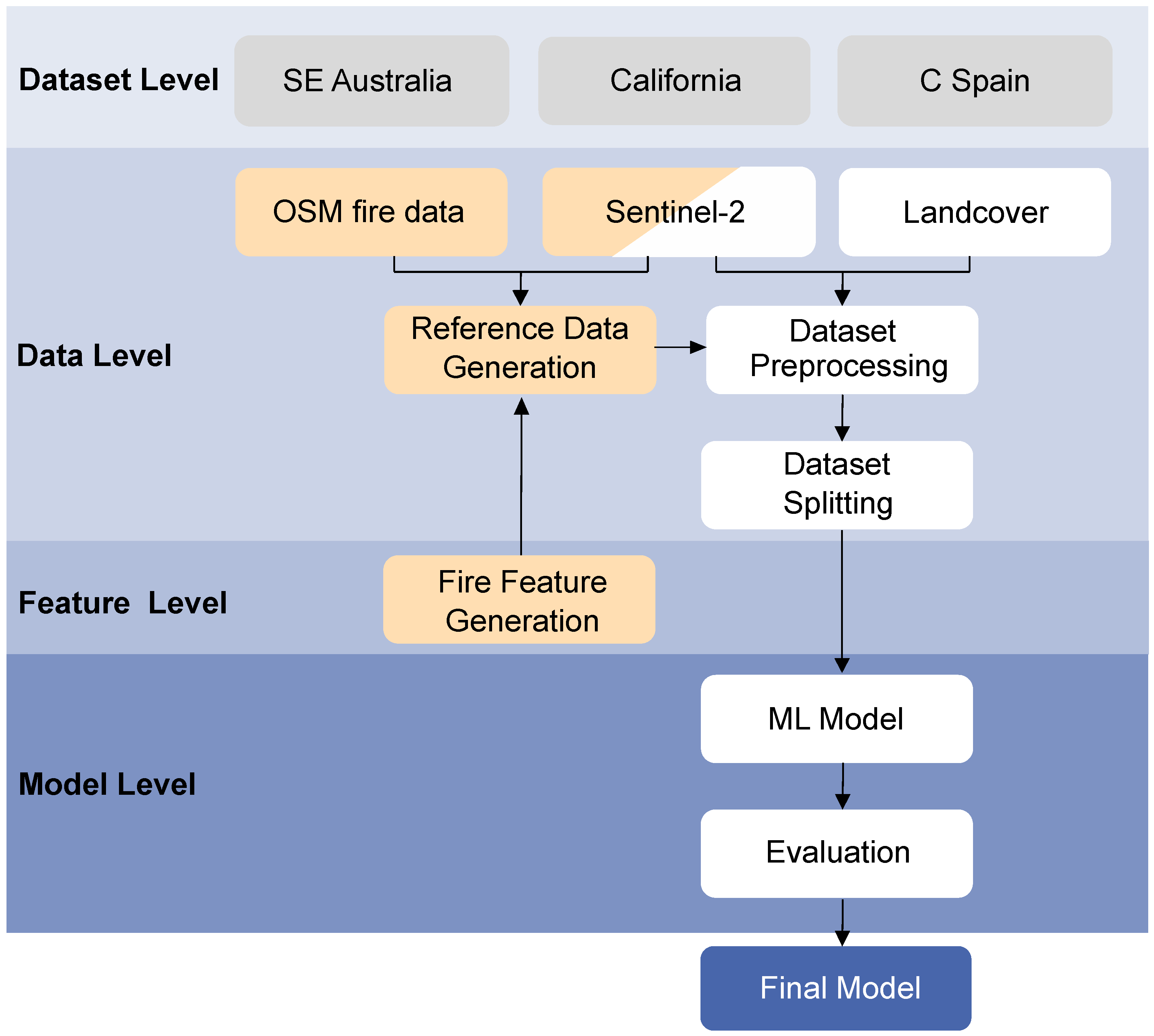
Since detecting active fire and mapping burned areas based on Sentinel-2 data comprise a supervised classification task, we conducted an appropriate workflow [63]. Figure 1 shows our applied combined classification framework of fire and burned areas structured into different levels. First, the data are described in the dataset level covering the exemplary study regions (Section 2.1) and the extracted datasets (Section 2.2). More specifically, the input data (Section 2.2.1), namely Sentinel-2 data, OpenStreetMap (OSM) fire data vector files, and land cover data, are summarized. The generated reference data are described next (Section 2.2.2) covering the feature level in Figure 1. Note that we refer to the combination of input features and desired output data as a data point. At the data level, the generated datasets were processed and split (see Section 2.2.4), which was necessary for the ML models’ training and evaluation. Finally, the selected ML models, their optimization, and the model evaluation metrics are stated in Section 2.3. These parts are included in the model level of the classification framework.

Figure 1.
Visualization of the combined classification framework of fires and burned areas divided into the dataset level, the data level, the feature level, and the model level. The following abbreviations are used: SE—southeast; C—central; ML—machine learning.
2.1. Selected Study Regions
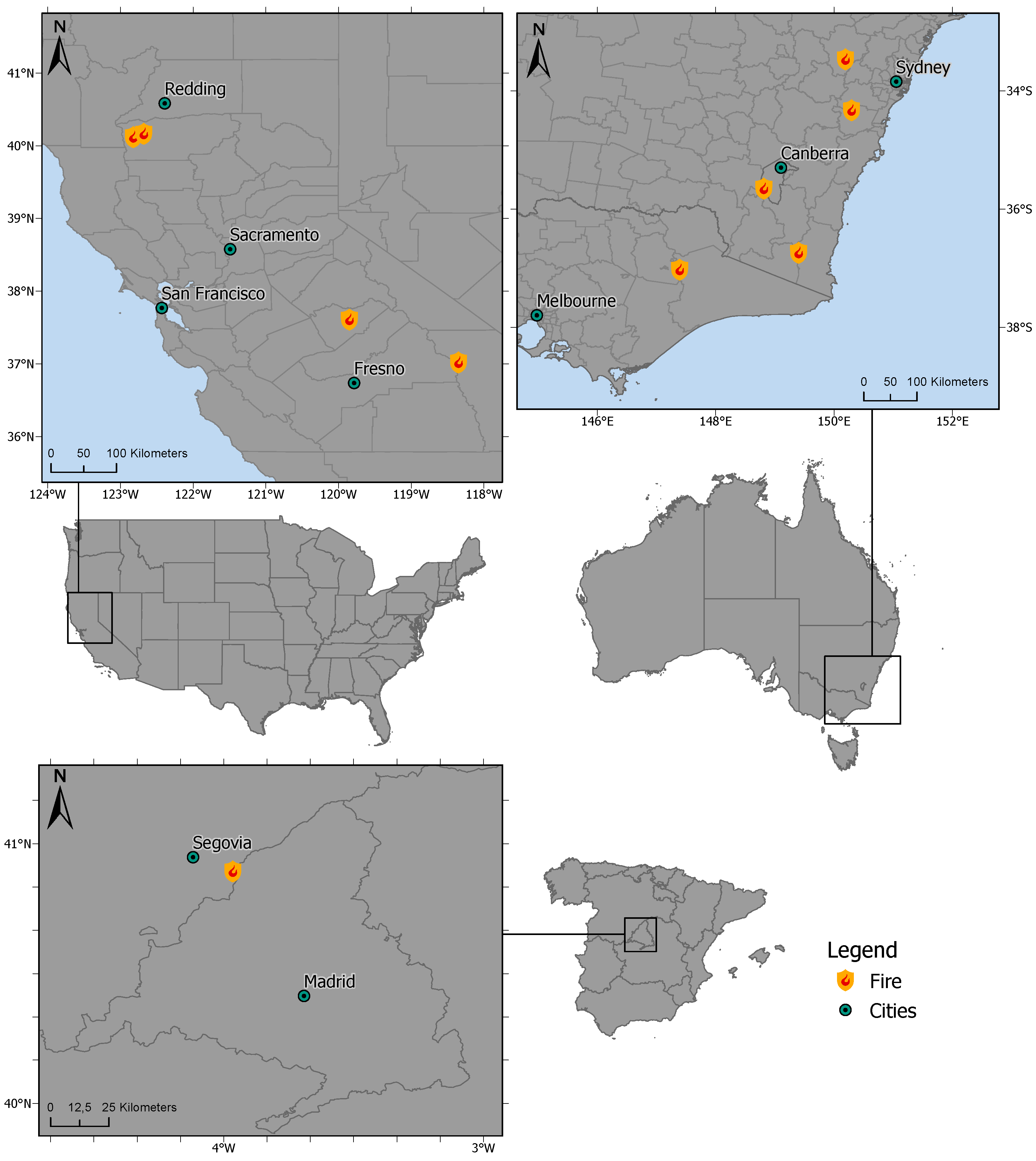
Since we aimed to develop a generic approach including supervised ML models for fire detection and burned area mapping, the selection of the study area had to meet two main criteria. First, the study area should include different regions worldwide characterized by big fires in the last few years. Second, a variety of land use and land cover classes should be part of these selected regions. Therefore, we relied on two big fires in two different regions and countries: California (United States of America (USA)) and the southeast (SE) of Australia (States of Victoria, Australian Capital Territory, and New South Wales). Figure 2 visualizes the locations of the fires used for the training, validation, and testing of the ML approaches. Detailed information about the distribution of the training, evaluation, and test data subsets concerning the different regions is given in Section 2.2.4. The specific fire sites were selected as well distributed within the regions matching the second-mentioned criterion. In sum, four areas in California and five areas in Southeast Australia, mainly containing different land cover classes, were used in the ML process. Besides, to evaluate the generalization abilities of the selected ML models, an additional study area was selected located in the central region of Spain (see Figure 2). Here, one area was chosen for the testing process.
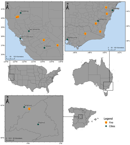
Figure 2.
Visualization of the selected areas in the USA (top left) and Australia (top right) used for the training, validation, and testing of the ML approaches and the areas used as the unknown test dataset in central Spain (bottom left). Data basis: © 2018 GADM. Projection: WGS84.
2.2. Data Basis, Generated Datasets, and Their Preparation
As mentioned before, the framework in Figure 1 structures the task into four levels by following a typical ML pipeline. In this subsection, we focus on the data and feature levels. First, we describe the input data (Section 2.2.1). The feature level contains the feature extraction necessary for the reference generation (Section 2.2.2), which is described next. After the reference generation, the preprocessing and the dataset splitting at the data level are necessary before being input into the ML model.
2.2.1. Input Features
We relied on three types of input data. Firstly, OSM data were used, which were acquired from national agencies. These data were only used to generate the reference showing unburned and burned area, which was necessary for training and testing of a model (see Section 2.2.2 for more details). Fire OSM data were not available in a generalized database. Therefore, the data were acquired for every region of interest from the responsible governmental agency, e.g., CalFire (CA, USA) or data.gov.au (accessed on 1 December 2021) (Australia). These data are provided in vector files, showing the extent of a fire (burned) area. For example, CalFire provides a multi-agency statewide database of fire history. Timber fires of ≥10 acres, brush fires of ≥30 acres, and grass fires of ≥300 acres are included. The database provides information about wildfire history, prescribed burns, and other fuel-modification projects [64]. For each fire perimeter, metadata such as the fire name, id, size, and objective are included by the responsible authority. Such data have been used as reference data in various studies (e.g., [32]). The vector data vary, depending on which agency they are provided by, concerning the temporal resolution and availability. For example, some vector files capture the outermost extent of accumulated burned area for one time step and current data are available every couple of hours (e.g., three hours for data.gov.au (accessed on 1 December 2021)). Other vector files capture the extent of one fire event that might have occurred for several days in a row, but data are only available once.
Secondly, we employed optical remote sensing data in the form of Sentinel-2 data. The information in the Sentinel-2 bands was the main feature used for the classification of the fire classes. We used Sentinel-2 data to benefit from the high resolution of 10 m, given for at least 4 of its 13 spectral bands. The selected scenes are made available on the satellite mission’s download platform (Copernicus Open Access Hub) and via a Python application programming interface (API), called SentinelAPI. Newer Sentinel-2 products are provided as Level-2A bottom-of-atmosphere (BOA) directly. The different bands have different spatial resolutions of 10 m, 20 m, and 60 m. In Level-2A products, the cirrus Band 10 is omitted, as it does not contain surface information, so in summary, 12 spectral bands were used in this study. All bands were resampled to a 10 m resolution.
Finally, a land cover product was also acquired from an API. The land cover product was used as an additional input feature since different underlying land cover classes change the spectral reflectance of the classes of Fire, Burned, and Unburned. For example, a burned forest has a different spectral signature than a burned grassland. Thus, the ML approaches can learn during the training that several different burned land cover classes still correspond to the class Burned despite their spectral differences. The worldwide-available product Copernicus Global Land Cover Layers (CGLS-LC100) Collection 3 with a 100 m resolution was used [65]. It is available from 2015 to 2019, as well as being updated yearly. The product is assessed via the GoogleEarthEngine Python API [66] and provides several bands for which the discrete classification is used, which includes 23 primary classes. The land cover classes are defined according to the CORINE (Coordination of Information on the Environment) Land Cover class definition. They are consistent over the entire globe. The product is derived from the PROBA-V 100 m time series. The land cover data were interpolated to a 10 m resolution by nearest-neighbor interpolation to retain discrete class values. Thus, its resolution corresponds to the resolution per pixel of the Sentinel-2 data. From the combination of the above input features, we obtained 13 input features in sum, containing 12 Sentinel-2 bands ignoring Band Number 10 and 1 land cover feature for each selected Sentinel-2 pixel. Note that the OSM data were only used for generating the reference data and not as input features for the ML approaches.
2.2.2. Generated Reference Data
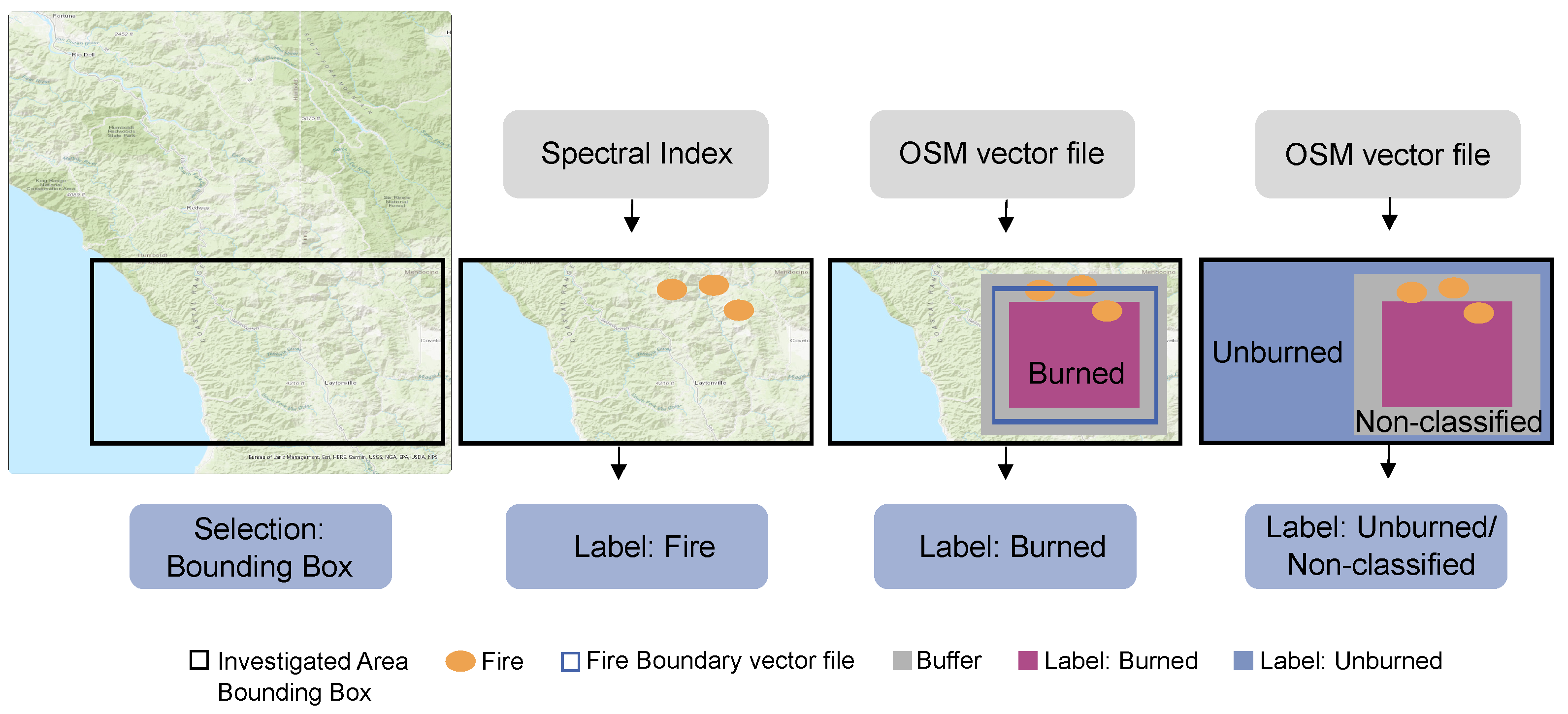
When applying supervised ML approaches, appropriate and sufficient reference data are needed. For our study’s aim, it was indispensable to have a reference dataset that allowed differentiating the classes of unburned areas, burned areas, and areas of actual fire. However, for this specific classification, no benchmark dataset was available at the required resolution (a high spatial resolution of 10 m for Sentinel-2 data) for the target classes of Fire, Burned, and Unburned. Therefore, we created a respective dataset with all data points containing single pixels of the Sentinel-2/land cover image with 13 input features (attributes) and the corresponding labels of the target class. In the following, we summarize the steps to generate the reference data (labels), before describing them in detail below. Figure 3 shows Steps 1 to 4:
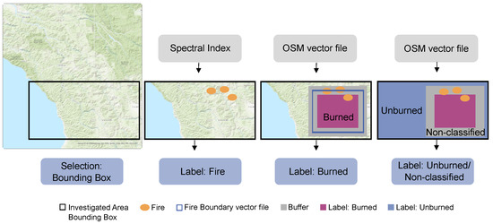
Figure 3.
Visualization of Steps 1 to 4 of the reference generation. Base map: ESRI ArcGIS Pro. Projection: WSG84.
- 1.
- Select a specific region of interest inside the study region (Section 2.1) by applying a bounding box, for which information on burned and unburned areas provided by OSM data is available;
- 2.
- Detect an active fire area based on spectral indices. The detected pixels are labeled as Fire;
- 3.
- Detect a burned area based on OSM data. The detected pixels are labeled as Burned;
- 4.
- Finally, label the rest (neither fire nor burned) of the pixels within the bounding box as Unburned or Non-classified.
First, Step 1 requires the available and downloaded OSM data providing information about fire areas or burned areas. Then, according to its size and the date of fire appearance, a specific fire site was chosen inside the Section 2.1 study regions from the OSM data. Simultaneously, we obtained the corresponding Sentinel-2 data of the selected region of interest several days after the set fire start date, providing reference data for burned areas. We also examined if actual fires were present in the available Sentinel-2 images, providing reference data for currently burning areas. For visual fire detection, false-color images of the NIR (Band 8a) and SWIR (Band 11 and Band 12) bands are most helpful. Thus, fires are well-detectable in the first days after the fire incident started. Concluding Step 1, we relied on areas that were detected as fire or burned areas visually and used these areas for further processing. We define a specific bounding box within this region of interest in Step 1. The corresponding Sentinel-2 image and OSM data were subsetted to the extent of this bounding box. All data points, respectively pixels, within this bounding box were labeled in the following steps.
For an automatic active fire detection in Step 2, several indices can be applied according to other studies (see Section 1.1). In pre-studies, we evaluated most of the proposed indices to select the most appropriate index for our task, the fire detection with Sentinel-2 data. We relied on the so-called Active Fire Detection (AFD) Index 3 (), according to Cicala et al. [15]. This index is regarded as most beneficial for the detection of highly energetic fires. At the same time, it is also useful for blazing, glowing, and therefore, less-energetic fires. It is calculated as follows:
where and B for band. was derived experimentally for each investigated region (Spain: 0.9, California: 0.5, Australia: 0.5).
The indexing was applied for all pixels inside the bounding box created in Step 1. We subsequently applied thresholding. If the pixels’ values were higher than the experimentally derived threshold of 5, we labeled these pixels as Fire. The rest of the pixels inside the bounding box remained unlabeled in this step.
In Step 3, we selected the pixels that covered the burned area. Therefore, we referred to the OSM data vector files as a reference for burned areas. To ensure that the pixels of the Fire and Burned/Unburned areas were not blended accidentally, we set a buffer zone around the vector file. The buffer size depended on the actual size of the OSM data vector file for the fire in question. About a 100 m to 300 m buffer size was usually applied. Pixels within the OSM area, but outside the buffer were then labeled as Burned areas. They were also reviewed, not to be accidentally labeled as Fire by comparison with the fire labels of Step 2.
Finally, in the last step, we needed to label the remaining pixels inside the bounding box area that had not been labeled yet. A pixel was already labeled as Fire if it was classified as fire by the AFD-3 index according to Step 2. A pixel was already labeled as Burned if it was located within the OSM boundary, not classified as fire, and not located within the buffer zone according to Step 3. The label Non-classified was provided for pixels located within the buffer and not labeled as fire. For these pixels, we could not be sure to which class they truly corresponded from the references that were available to us. We discarded these pixels to obtain only pure data points as the input for our models. Eventually, we labeled pixels outside the OSM boundary and outside the buffer as Unburned.
For classification improvement and generalization purposes, we included pixels of the Unburned classes that covered water and settlement areas. These particular pixels were characterized by spectral differences and occurred only in a reduced number. The main reason was that fires and burned areas appeared primarily in forested regions in which these two land cover classes were relatively rare.
2.2.3. Dataset and Imbalance
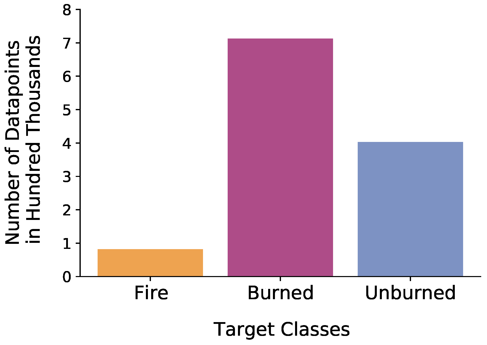
As we selected different study areas mentioned in Section 2.1, several subsets of data points per region existed. In the next step, we combined all subsets into one dataset containing 9 million data points.
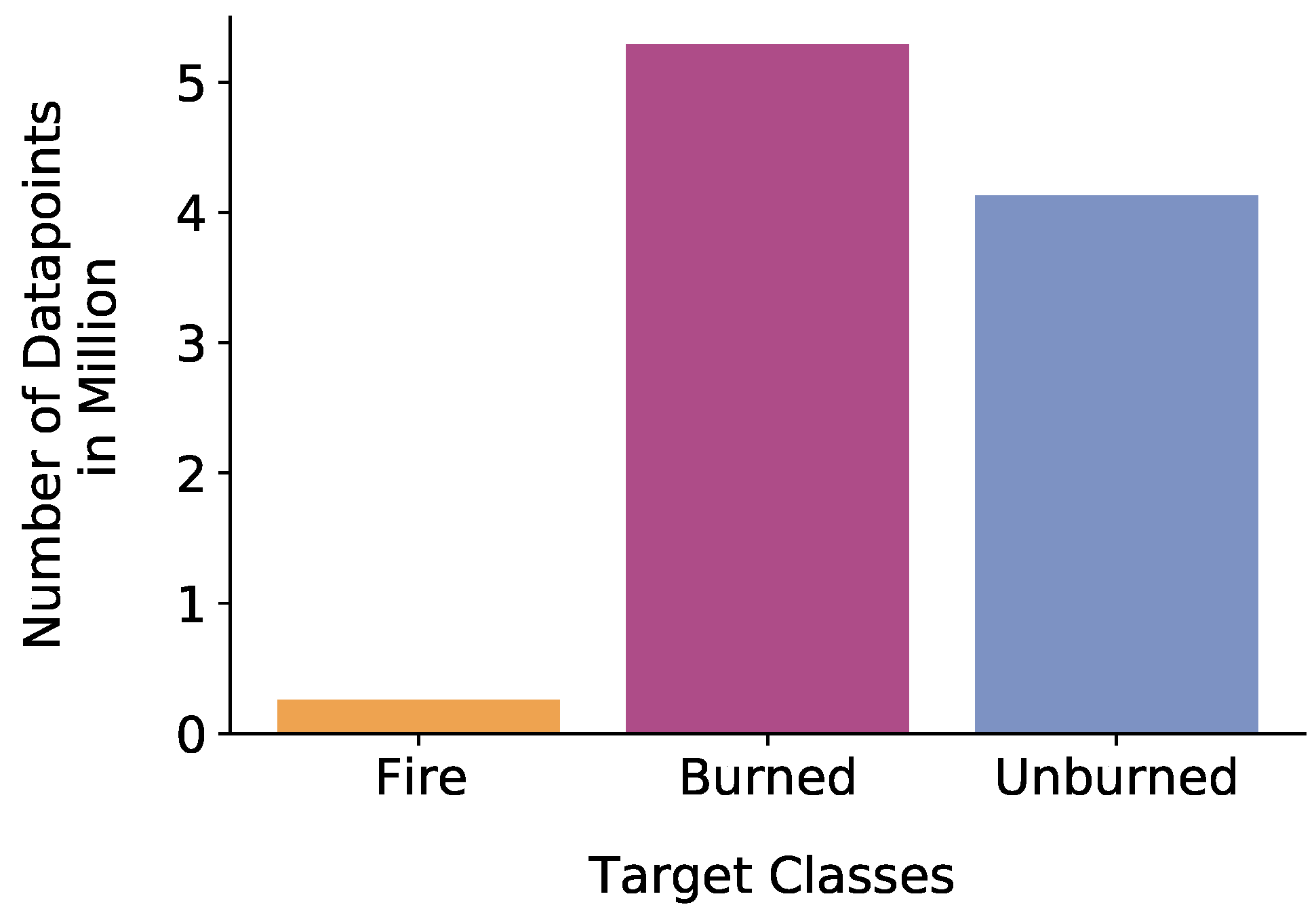
The created datasets were between-class imbalanced concerning the target classes of Fire, Burned, and Unburned area (see Figure 4). Overall, fewer pixels appeared in the satellite images as fire pixels, as active fires happen to occur for a short amount of time. While the state of non-burned area exists continuously, the state of burned area exists at least as long as it takes for local vegetation to regrow. This fact led to the class of Fire being underrepresented in the dataset. The imbalance might led to a non-optimized result for the Fire class. However, this is the most valuable class to be predicted for the aim of fire management and should not be neglected. Besides, more data points were required for the Unburned and Burned classes, as the underlying land cover classes had a higher impact on the spectral reflectance for these classes to be distinguished in contrast with the Fire class. The spectral reflectance of fire pixels was not influenced as much by the underlying land cover class since the reflectance of fire is unique in Bands 8A, 11, and 12.
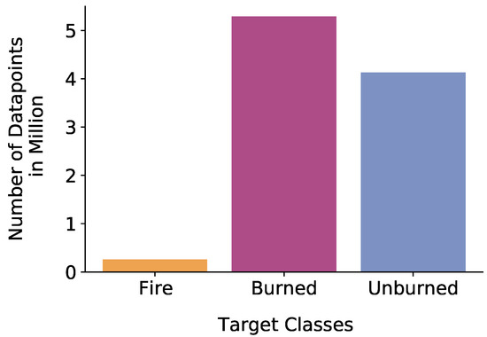
Figure 4.
Distribution of data points of the whole dataset combined from all study regions per target class.
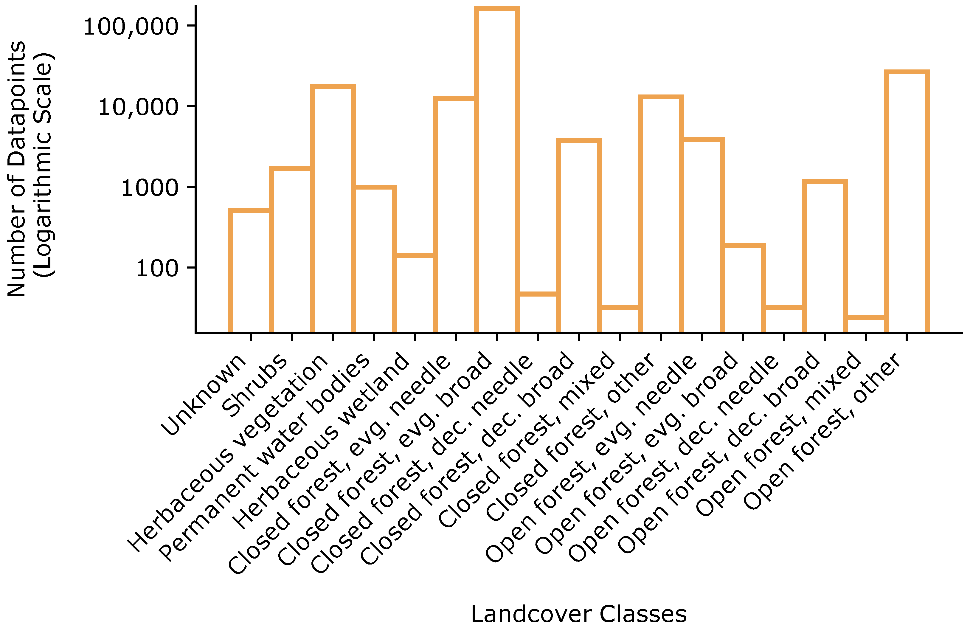
Apart from the between-class imbalance, an imbalance between land cover classes within the three target classes existed. Some land cover classes occurred much more frequently than others in general. Figure 5 shows an exemplary distribution of the data points per land cover class within the target class of Fire. Even moderate levels of class imbalance have an impact on the performance in classification problems [67,68]. To reduce the imbalance of the dataset, we applied undersampling [69] as a preprocessing step (see Section 2.2.4).

Figure 5.
Distribution of data points of the whole dataset combined from all study regions per target class Fire and land cover class on a logarithmic scale.
2.2.4. Dataset Preparation, Splitting, and Undersampling
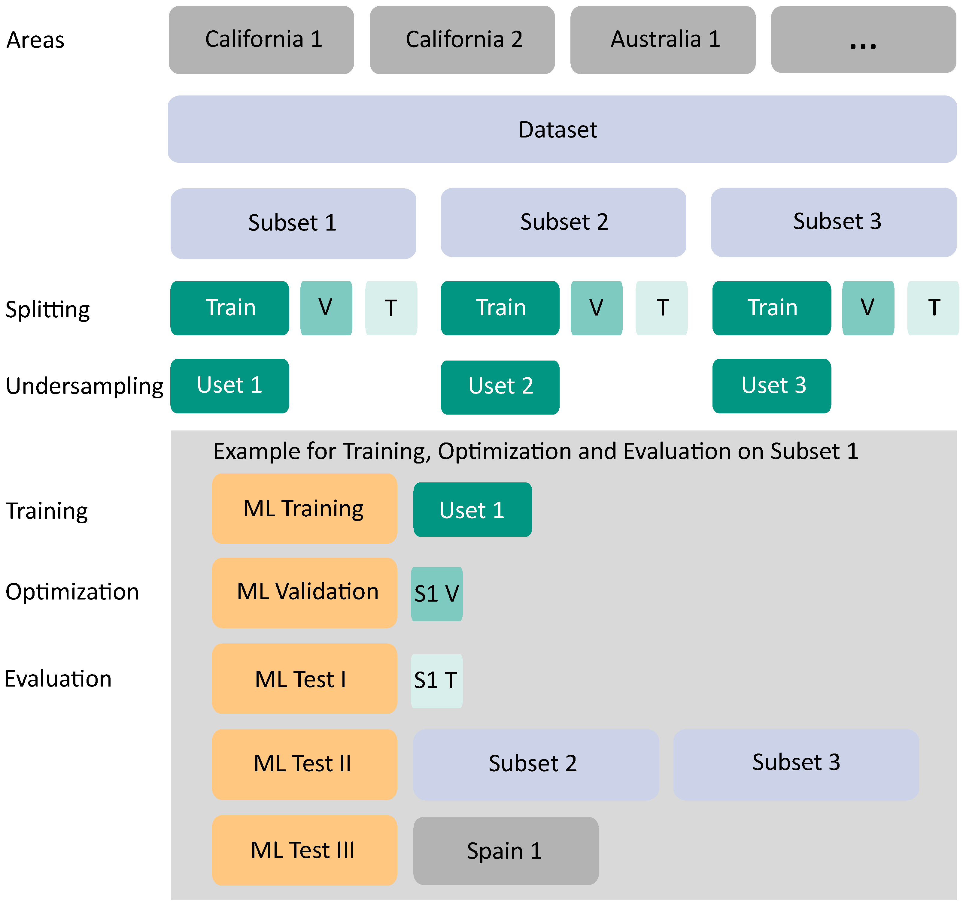
After generating the reference data and defining the datasets, we prepared the dataset and split it for the ML application (see Figure 6). By dividing this dataset into three equal subsets (Subset 1 to 3), we decreased the computational cost during the training phase of the ML approaches. A second aspect of this initial splitting is given in Section 2.2.3, explaining the between-class imbalance of the dataset. We split the basic dataset randomly, but guided this to ensure that every subset consisted of approximately the same number of data points per land cover class. This process was essential since some land cover classes were less represented.

Figure 6.
Flow diagram summarizing the dataset preparation applied in this study with the ML process example illustrated for Uset 1. The following abbreviations are used: Uset—undersampled set; V—validation set; T—test set; S—Subset; ML—machine learning.
Furthermore, an independent splitting of the subsets into the training, validation, and test datasets was necessary when evaluating each model’s classification performance. Therefore, we randomly split each subset dataset into three sets with a ratio of 60:20:20 (see Figure 6). Standard ML guidelines were followed with the chosen split ratio (see e.g., Kattenborn et al. [70]), and the randomized split guaranteed an independent distribution of the subsets. The training dataset was reserved for the respective ML model’s training, while the evaluation of the model was conducted on the test dataset. Besides, the model’s hyperparameters were optimized on the validation dataset.
Next, we applied a selected undersampling approach. Undersampling approaches are efficient to deal with in-between class imbalance [69]. To ensure a more balanced dataset, the subsets’ training sets were formed by deleting instances of the majority class [71]. Since the datasets comprised many data points, even for minority classes (see Section 2.2.3), the undersampling approach was appropriate for balancing the dataset. Note that the undersampling approach was only applied for the three training subsets to ensure the validation/test set reflected the original distribution of the data points. Basic random undersampling might deteriorate the existence of data points of rare land cover classes, as potentially helpful information in the ignored examples might be neglected. Therefore, we selected an informed undersampling approach concerning the land cover classes.
As a result, an undersampled training dataset of each original training subset was created by randomly undersampling only data points of the majority land cover classes inside the majority targets, unburned and burned classes. We refer to these three undersampled training subsets as Uset 1 to 3 (see Figure 6). Data points of the regular land cover classes were undersampled until they reached a threshold of N data points, similar to an EasyEnsemble approach [69]. Then, we chose an experimentally derived threshold per land cover class per target class (only on the Unburned and Burned data points).
The training of the ML models on these three datasets separately ensured the robustness and reproducibility of the subsequently performed classification. After the applied undersampling, the overall amount of data points for the two target classes, Unburned and Burned, was still higher than for the target class Fire (see Figure 7). These differences were not equalized, as they reflected the appearance of the classes in reality. Table A1 (see Appendix A) gives the number of data points per class and their distribution after the splitting and, in addition, after applying the undersampling approach. Note that we refer to the dataset resulting from the undersampling as Usets. Each Uset was used once as a training dataset during the ML models’ training. Figure 6 shows the workflow example for Uset 1. After the training run with Uset 1, the same was carried out for Uset 2 and Uset 3.

Figure 7.
Distribution of data points of an undersampled subset (Uset 1) per target class after balancing with a slightly lesser imbalance than the original.
With the exemplary workflow, we ensured an extensive evaluation of the applied ML approaches that focused on investigating the performance and generalization abilities on different, locally distinct datasets. Besides, each trained model was validated three times:
- The Uset was used for training the ML approach, and the validation was conducted with the validation set of the respective subset;
- Then, Test I testing was conducted with the test set of the respective subset;
- The total of the two other subsets was used as further test data in Test II. For example, in the case of Uset 1, Subset 2 and Subset 3 were used as test datasets;
- For a completely independent evaluation in Test III, the dataset created for the selected region of Spain, in the training and testing steps a so-far unseen region, served as an additional test set.
In summary, all subsets (Test I and Test II) and the unknown Spain dataset (Test III) were used for each evaluation process of the ML approaches depending on the training on the respective Usets. Table 4 displays the number of data points of the respective test datasets applied to evaluate the ML approaches trained on Uset 1 (see Figure 6).

Table 4.
Number of data points (Sentinel 2 pixels) of the respective test datasets used for evaluation the applied ML approaches. The numbers are exemplarily illustrated for the training on Uset 1 according to Figure 6.
For some supervised classification approaches, further data processing was necessary. For example, scaled input features are required for artificial neural networks (ANNs) and highly recommended for SVMs. Thus, scaling was applied to the datasets beforehand for any ANN and the SVM in Section 2.3.
2.3. Methods
In this subsection, we describe the model level including supervised ML models to solve the underlying classification task (see Figure 1). As shown in Figure 1, the model level represents the last level in the classification framework. The deployed ML models are presented in Section 2.3.1. Subsequently, we summarize the evaluation metrics in Section 2.3.2.
2.3.1. Machine Learning Models for Classification
As mentioned in Section 1.1 and Table 2, several supervised learning approaches exist using Sentinel-2 input data to predict classes such as Fire, Unburned, or Burned successfully. These approaches comprise, for example, tree-based models, SVMs, or DL such as convolutional neural networks (CNNs). However, the objective of this study was to evaluate the classification performances of such ML approaches to predict all of the three defined classes in one pass. Therefore, we selected shallow learning approaches such as extremely randomized tree (ET) [72], AdaBoost [73], gradient boosting (GradientBoost) [74], multi-layer perceptron (MLP) [75], supervised self-organizing map (SOM) [63,76,77,78], and SVM with bagging [79]. Besides, we relied on a one-dimensional (1D) convolutional neural network (1D-CNN), which was similar to the DL approach of Riese and Keller [80]. The selected ML approaches were chosen since their robustness and strong classification abilities have been proven in similar classification tasks and pre-studies (see [31,59,81]). Table A2 in Appendix B summarizes all applied ML models with their respective hyperparameter settings. Note that we only applied scaling as preprocessing for the DL approaches and BaggingSVM.
ET, AdaBoost, and GradientBoost were applied as tree-based classification models and were associated with decision trees (DTs). Generally, they included a root and a leaf node. Root and leaf nodes were then linked by branches. During the training of DTs, the data of the respective dataset were split at every branch. With these splits, subsets were generated, which highly correlated with the 13 input features. For example, RF is defined by an optimum split, while ET relies on a random split, which reduces variance, according to Geurts et al. [72]. Details on the structure and setup of the models were presented in the corresponding studies [72,73,74].
Most of the SOMs are applied in an unsupervised manner as clustering approaches [78,82]. For the underlying classification task, we relied on the supervised classification SOM introduced by Riese and Keller [63]. In sum, the supervised classification SOM contains an unsupervised and a supervised SOM. The unsupervised SOM part selects the best-matching unit for each data point. Selecting the data points was implemented randomly. Then, the learning rate, neighborhood function, neighborhood distance weight matrix, and class-change probability matrix were calculated. In contrast, the supervised SOM connects the selected best-matching unit to a specific class. Note that the weights of the supervised classification SOM consisted of a class. The SOM weight matrix was modified, and the process was repeated until the maximum number of iterations was reached. Details of the supervised classification SOM were given in Riese and Keller [77], while the Python implementation can be found by Riese [83]. Besides, the hyperparameters of the supervised classification SOM are presented in Table A2.
Another ML approach included in the model level was SVM. We propose an SVM ensembles approach with bagging. In this specific case, each SVM was trained independently with randomly chosen training data points. Finally, these SVMs were aggregated into the collective SVMbagging [79]. This proposition was advantageous since the standard SVM storing the kernel matrix requires memory, which scales quadratically with the number of data points. So far, except for the classification SOM, the ML models were implemented with the Python package scikit-learn [84].
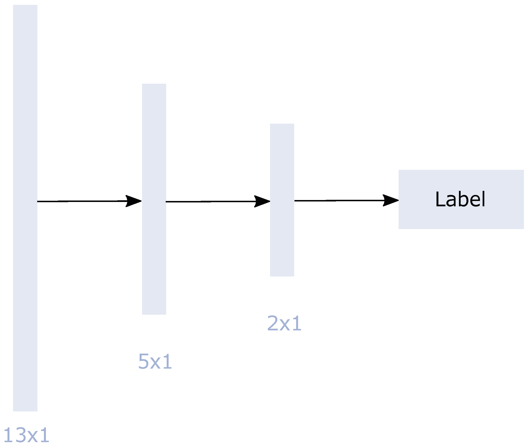
As an ANN approach, we used MLP. MLP consists of a simple architecture with one input, at least one hidden layer, and one output layer [85]. Each node, except the input node, is a neuron that uses a nonlinear activation function. Backpropagation is applied for training. Figure 8 shows the standard scikit-learn-implemented [84] MLP architecture with the chosen hidden layer sizes of 5 and 2. The input layer consisted of 13 neurons representing our 13 input features.

Figure 8.
Flowchart of the MLP architecture for the 13 input features during the training process. The network includes two hidden layers. The implementation is a standard architecture with the selected hidden layer size using scikit-learn [84].
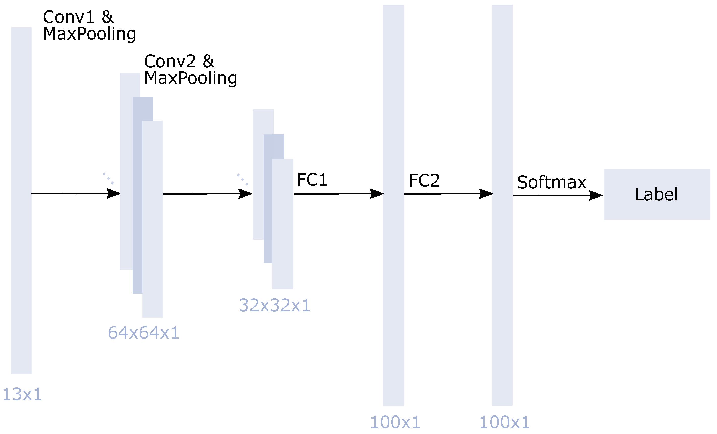
Since CNNs have achieved good classification and regression results on remote sensing images and spectral data [86,87], we also applied a CNN architecture. More precisely, we employed a 1D-CNN since the generated reference data points were extracted pointwise. A standard 2D-CNN, therefore, was not applicable. The idea to deal with pointwise reference data with the help of a 1D-CNN was adapted from Riese and Keller [80]. Generally, a 1D-CNN is resilient against any noise occurring in the Sentinel-2 data. Based on a 1D-CNN’s deep layers, several features were created out of the 13 input features. The architecture was similar to the one implemented in Riese and Keller [80]. However, it was adapted during the training process and optimized for the task. Figure 9 shows the implemented 1D-CNN architecture. It consisted of two convolutional layers, one with a filter, the other with a filter. Each convolutional layer was followed by a max-pooling (MaxPooling) layer. Finally, two fully connected (FC) layers were implemented with 100 neurons each. In addition, the last FC layer was combined with a softmax activation function. Except for this last activation function, the ReLU function was used (see also Table A2). The Adam optimizer was used. The CNN’s hyperparameters were optimized with a Hyperband tuner, which is a variation of random search. It is fast due to adaptive resource allocation and early stopping [88]. The 1D-CNN was trained five times with the best possible model. This model was chosen according to the highest validation accuracy, which was calculated during the training process on the validation data. The results of the five runs were averaged.
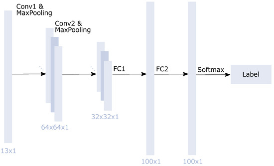
Figure 9.
Flowchart of the 1D-CNN architecture for the 13 input features during the training process. The network includes convolutional (CONV), fully connected (FC), and max-pooling (MaxPooling) layers. At the end of the network, a softmax function is applied.
2.3.2. Accuracy Assessment
For the evaluation of the models’ classification performances and the comparison of the different results, we relied on several metrics. Concerning the reference data, the prediction for a data point was either true positive (TP), true negative (TN), false positive (FP), or false negative (FN). The applied metrics were implemented in the scikit-learn [84] package. Besides, we had to consider that metrics were applied that could cope with an imbalanced multiclass classification problem. For example, the balanced accuracy (BA) defines such a metric suitable for imbalanced datasets. Overall accuracy (OA), Cohen’s coefficient, precision, average accuracy (AA), and the F1-score are additional metrics that are usually applied in classification problems. Note that i represents a respective data point. All evaluation metrics were implemented in scikit-learn [84] and are summarized as follows:
- OA represents the proportion of correctly classified test data points among all other data points and is calculated according to Equation (2).
- measures the agreement between two raters, each f which classifies each data point. It is considered a more robust measure since it considers the possibility of agreement occurring by chance. The two terms included in Equation (3) are the observed agreement among the raters (which is the above-mentioned overall accuracy (OA)) and the hypothetical probability of agreement by chance .where:and represent the sum of the products of the row total and the column total sum of each class, which can be calculated by summing the row and column values for each class in the confusion matrix;
- Precision (also correctness) predicts the positive values.
- Recall (also completeness) rates the TP and is necessary to calculate the F1-Score. Note that we excluded the recall in the Results Section (see Section 3).
- AA equals the weighted Recall in a multi-class classification problem. We therefore only included the AA in the Results Section (see Section 3). The weighted Recall is calculated from the classwise Recall calculated in the earlier step;
- The F1-Score is a metric of the test’s accuracy. It considers the Precision and Recall of the test subset to compute the harmonic mean.
- BA gives information about how well a class is classified by the respective ML model. Moreover, it is class imbalance suitable since it takes into account the individual classes’ sizes [89].where is the true label of the i-th data point, is the corresponding weight, and is the predicted class label.
3. Results
In the following sections, we present the classification results. Section 3.1 focuses on the overall classification performance of all applied ML models. Next, we show the several models’ performances concerning the different created subsets and the classwise performance of the models (see Section 3.3). Finally, Section 3.4 presents the generalization evaluation of the ML models on an entirely unknown and geographically independent dataset. Thus, we can investigate and assess the classification performances of our presented approach for a concurrent and combined fire and burned area detection in detail. Note that comparing our approach’s classification results with other approaches was unfeasible due to the lack of existing approaches combining fire and burned area detection on one task (see Section 1.1).
3.1. Overall Classification Performance of the Models
Table 5 shows the prediction scores of the applied ML models on the selected Subset 2. In this case, the models were trained on Uset 3 (see Figure 6 for details). All selected ML models achieved very high prediction scores. The 1D-CNN and ET showed the best classification results with an OA above 97%. The supervised classification SOM produced the least-accurate results with an OA of 87%, followed by AdaBoost with 91%. When considering Cohen’s , all models’ values ranged from 73% to 94%, with a slightly stronger differing value of 63% for the SOM approach. With 83% to 97% for all models, the precision was similar to the models’ OA values and the F1-scores. The AA score also ranged in similar values of 80% to 97% for all models. All models achieved high BA values (85% to 98%), especially ET and the 1D-CNN outperformed the other models with 98% (see Figure 10). The BA scores are also visualized in the normalized confusion matrices of Figure 10.

Table 5.
Classification metrics in % of all ML models trained on Uset 3 and their prediction performed on Subset 2 and compared to the reference data. The 1D-CNN scores were calculated as the average of five runs. The bold values represent the best classification results, respectively. (OA: overall accuracy, Prec: precision, AA: average accuracy, BA: balanced accuracy).
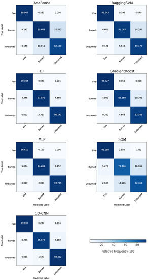
Figure 10.
Normalized confusion matrices for the applied ML models. The prediction was performed on Subset 2 and compared to the reference data. The ML models were trained on Uset 3.
ET achieved the best accuracies in the metrics OA and precision, while the CNN achieves the best results in the AA and BA. Further information concerning the confusion matrices is presented in Section 3.3.
3.2. Classwise Performance of the Models
The ML models’ classwise performance was evaluated on the test Subset 2, while the models were trained on Uset 3 (according to scheme of Figure 6). We can investigate the ML models’ classwise classification performance by displaying the confusion matrices introduced in Figure 10. According to Figure 10, all models could distinguish the three target classes well. The confusion of the classes Burned and Unburned by the SOM was slightly higher than by other approaches, as shown in Figure 11. It achieved the lowest classwise classification performance. In sum, the Fire class was classified the best by all models, with a BA score from 95% to 99%. The ET model and the 1D-CNN achieved the highest classwise accuracy when focusing again on the Burned and Unburned classes. ET classified the Burned data points better than the 1D-CNN (97.07% compared to 95.07%). However, for the unburned class, the 1D-CNN outperformed every other applied approach with 98.31%.
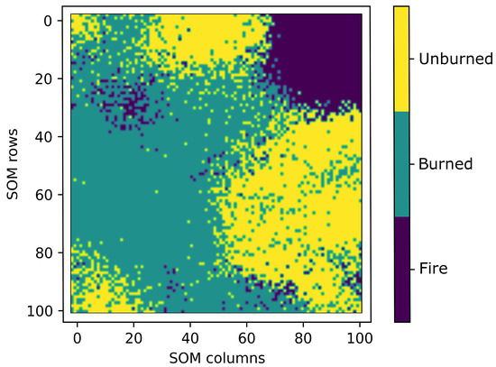
Figure 11.
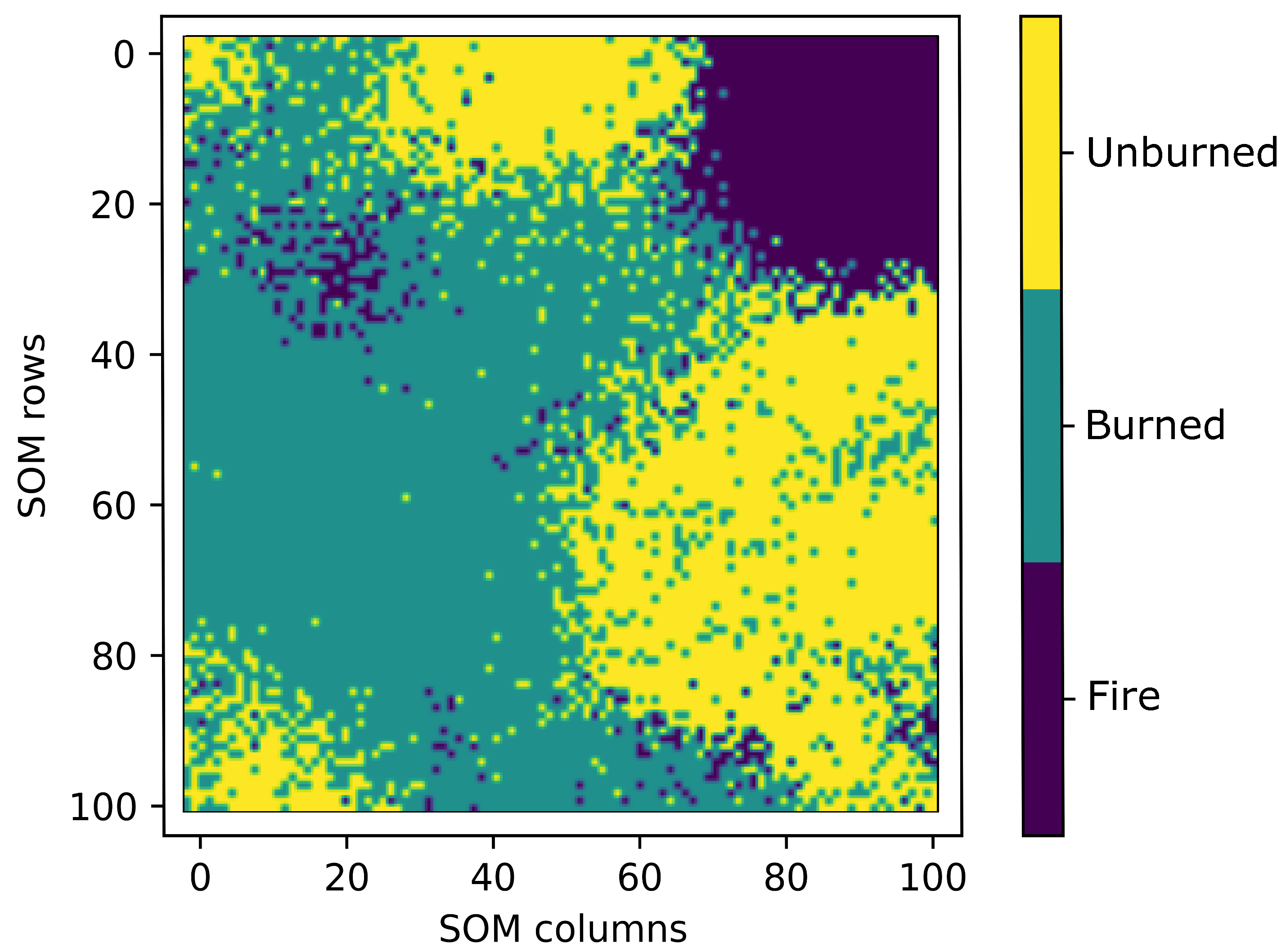
Visualization of the supervised classification SOM as the distribution of the classes linked to each SOM node as the output.
As investigated in pre-studies, the models’ classwise accuracies would be slightly lower, especially for the minority Fire class due to the imbalanced characteristics of the original dataset. These results are also shown in Figure A1 in Appendix C, where all models were trained on the training split of Subset 3 and evaluated on Subset 2 according to ML Test II in Figure 6. According to the confusion matrices in Figure A1 and Figure 10, the models achieved marginally better classification results on the balanced dataset. ET’s and AdaBoost’s classification results improved for all classes for the balanced dataset, while BaggingSVM’s and 1D-CNN’s results improved in two of three classes. However, the classification results for the class Fire improved through balancing in all models.
Although SOM’s classwise classification performance was moderate, SOM has one advantage concerning the interpretation of the classification results. SOMs can visualize the results of a classification in a two-dimensional (2D) output grid [76,78] as a clustering approach. Thus, we can (visually) extract information about the distinction between the three different classes in the dataset. Note that the other applied ML approaches cannot visualize the interclass variance, respectively classwise, in a human intuitively interpretable manner (2D grid). Figure 11 visualizes the distribution of the classes linked to each node of the supervised classification SOM. As a result, we can recognize that the class of Fire is located in the upper right corner of the 2D grid. Only a few data points occur outside this corner. Besides, the data points of the Burned and Unburned classes are slightly more mixed and cover the remaining parts of the SOM grid. We notice four main clustered parts of the Unburned class, while one inhomogeneous area of the Burned class is given.
3.3. Classification Performances Concerning Different Subsets
Since we obtained different subsets for the training, optimization (see Figure 6), and evaluation of the ML models, we needed to compare the models’ classification results on these subsets. Table 6 summarizes the AA scores of four selected models, which were characterized by low computational costs. They were trained on either one of the three Uset, while we evaluated their classification performances on the remaining Subsets.

Table 6.
Classification results of the four selected models on different training and test data subsets. The values represent the AA in %. The bold value represents the best subset combination classification results.
In total, the four selected ML models achieved satisfying and similar classification results on all Subsets. Regarding the ET model as the best classification model, the maximum deviation was 0.9% between the training on different Usets and the test in the remaining two Subsets. We note that training ET on Uset 2 and Uset 3 achieved higher OA scores if evaluated on Subset 1. On the other hand, AdaBoost’s performance deviated 1.3% when training on Uset 1 instead of Uset 3 independently of the Test Subset. Note that AdaBoost scored the lowest OA.
3.4. Application of Two Selected Models on an Unknown Dataset and Their Performances
We applied the two best classification models, ET and the 1D-CNN, in Test III. All approaches showed very good results in Tests I and II. However, since the objective of this study was to find a model to best classify fire and burned area, we could rely on only the best two models for this third and last evaluation. With this evaluation, we assessed our approach’s generalization abilities on an unknown dataset. This dataset consisted of a regional area in Spain, Europe, as described in Section 2.2. Table 7 summarizes the classification performances of the two models. The 1D-CNN performed a better classification than ET concerning all metrics. The OA scores were extremely high, with 99.6% for ET and 99.8% for the 1D-CNN.

Table 7.
Classification metrics of ET, the 1D-CNN, and the NBR for comparison on the unknown selected Spanish regional dataset in %. The bold value represents the best classification results.
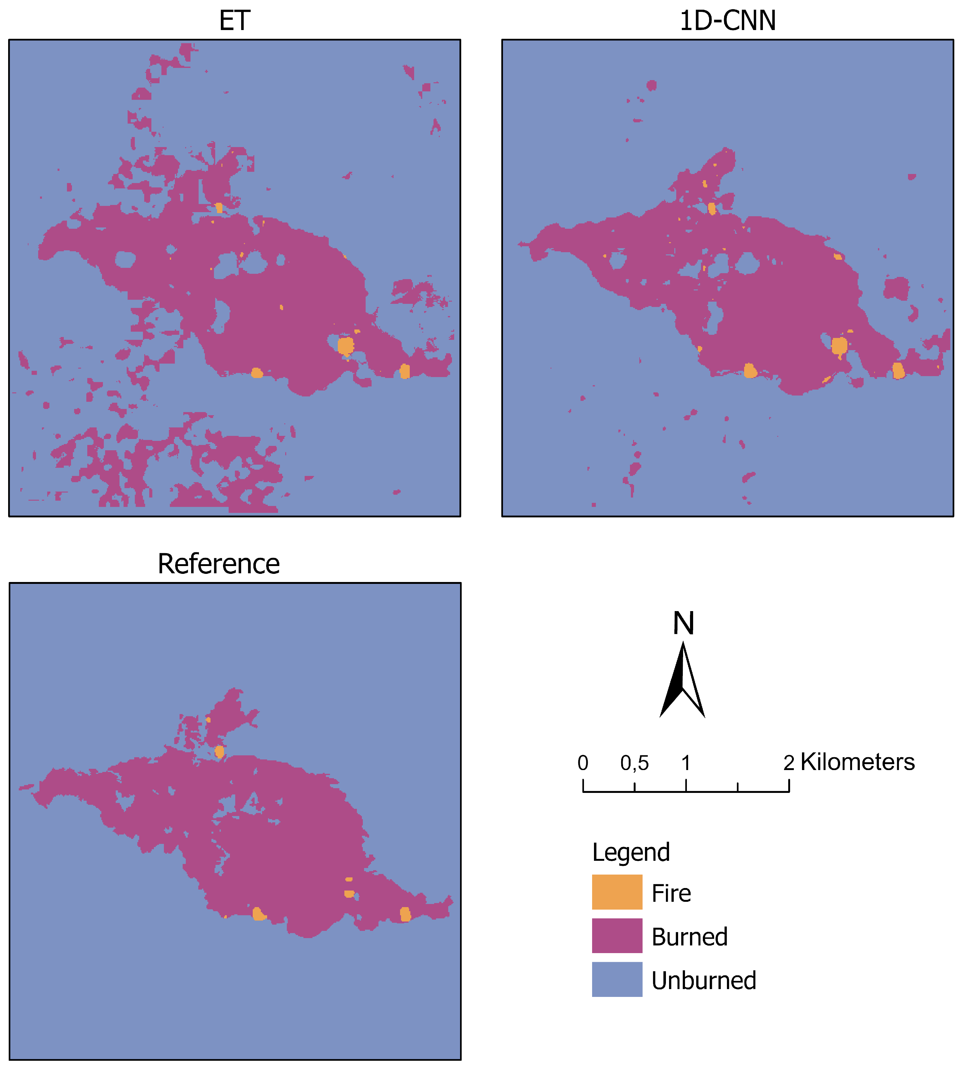
Besides, we visualize the classification results of ET and the 1D-CNN, as well as the reference data as maps in Figure 12. The results revealed that both models could accurately classify the burned area within the incident region, which was defined by the vector file boundaries. However, while the 1D-CNN generally corresponded better with the reference map, ET misclassified a few Unburned pixels as Burned outside the incident area. As for the class Fire, both ML models mapped these areas correctly, although they tended to classify more data points as Fire than existed in the reference dataset.
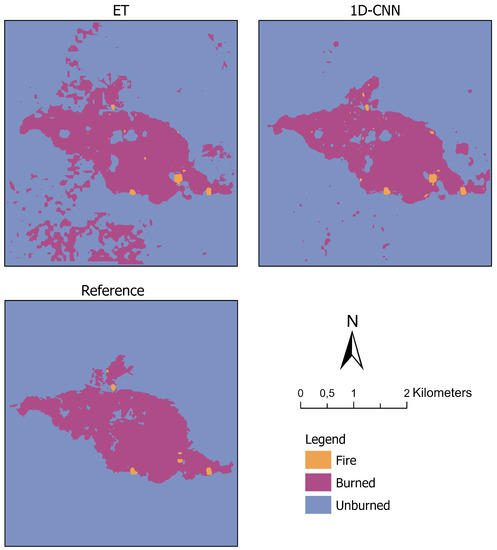
Figure 12.
Visualization of the classification results of extremely randomized tree (ET) (top left) and the 1D convolutional neural network (1D-CNN) (top right) on the independent test region in Spain. The visualization of the generated reference data is given on the bottom. Projection: Transverse Mercator.
4. Discussion
In this section, we discuss the presented study and the achieved classification results. First, we readdress the reference data generation for the combined detection of active fire and burned area (see Section 2.2.2), representing the first major challenge. Subsequently, we investigate the remaining challenges as stated in Section 1 according to the different results in the same order as shown in Section 3 (see Section 4.2, Section 4.3, Section 4.4 and Section 4.5).
4.1. Addressing the Challenge of Reference Data Generation for a Combined Detection
The supervised ML models require appropriate reference data to solve the classification task and detect fire and burned areas with Sentinel-2 data. Since these data were lacking, we needed to generate reference data. We relied on OSM data for generating reference data, which seemed to be appropriate for the detection of fires and burned areas. However, the selected OSM data need to correspond to the underlying and actual burned area state of the Sentinel-2 satellite data. Therefore, the OSM data selection could be a crucial aspect of the data pipeline (see Figure 1 and Figure 3); it was also performed manually. An additional challenging aspect was selecting the Sentinel-2 data used for the visual detection of the fires based on the false-color composite of Bands 8A, 11, and 12.
The required OSM and Sentinel-2 data must be of high quality. In sum, the reference data generation was conducted in a semi-automated manner and not as an entirely automated process and aimed at providing reference data for the combined detection of active fires and burned areas. This approach represents a limiting step of our entire workflow. Any classification results provided by the ML models can only be as precise as the reference data themselves. The accuracy of the generated reference data can only be evaluated visually. In our visual evaluation concerning the study’s generated reference data, we found that the used reference data were feasible for the underlying classification task. We received more than a few pixels labeled as Fire based on the applied index as a side effect. However, this effect did not interfere with the classification performances of the applied models.
4.2. Separation of the Classes Regarding the Models’ Overall Classification Performance
Overall, we noticed that some supervised ML models classified the three classes Fire, Unburned, and Burned better than other models. Although all models achieved high OA scores with more than 87%, a few models were outstanding with an OA score above 97%, such as ET and the 1D-CNN, referring to Table 5. ET represents a shallow learning ensemble approach, and the 1D-CNN is a deep learning approach. From the overall high classification metrics and the comprehensible 2D visualization of the SOM (see Figure 11), we understand that the underlying task of detecting fires and unburned areas in a combined approach is feasible based on the provided input features extracted from the Sentinel-2 data. When selecting the appropriate ML model, we suggest applying shallow learning approaches such as ET since they require less computation time and are relatively simple to train (less tuning of the required hyperparameters) compared to the deep learning architecture of a 1D-CNN.
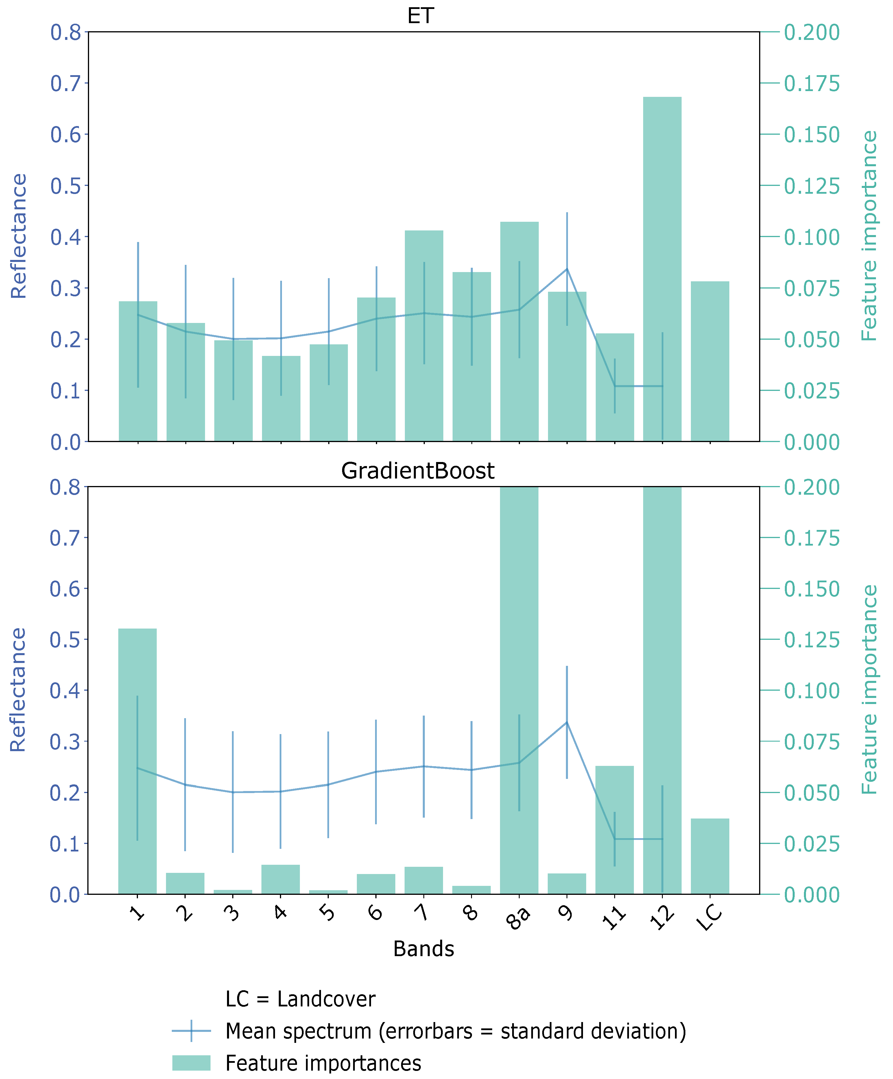
Concerning the various input features, the spectral information of the Sentinel-2 data combined with information about the underlying land cover represents the basis for the detection of fires and burned areas. For example, the spectral features were the most important for fire detection, while the land cover information indicated the distinction between burned and unburned areas. Figure 13 shows the feature importance of two ensemble approaches, ET and GradientBoost. As for ET, Sentinel-2 Band 12 was the most important feature, followed by Band 8A and Band 8. The additional land cover feature was the fifth important one in this case. The other remaining Sentinel-2 features were medium important.
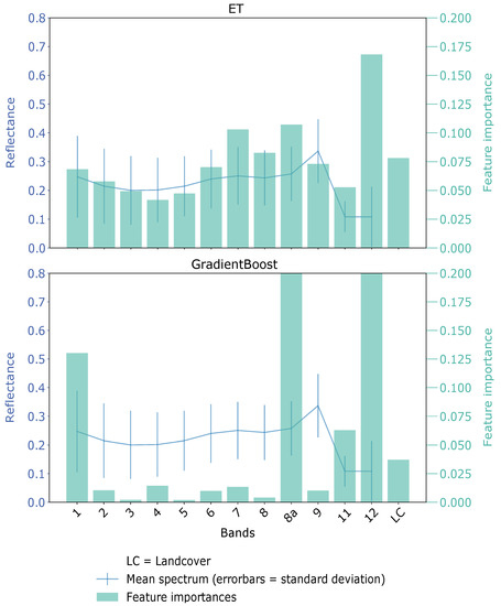
Figure 13.
Exemplary feature importance for extremely randomized tree (ET) (top) and gradient boosting (GradientBoost) (bottom).
For GradientBoost, the feature importance was more clearly ranked. The Sentinel-2 Bands 12 and 8a were the most important ones, followed by Band 1, covering the SWIR region and the land cover information. In conclusion, especially apparent in the GradientBoost, the SWIR bands and the land cover were the main important features. These features were also used for the active fire index calculation and generally for fire and burned area detection (see Section 1.1). The GradientBoost’s feature importance demonstrated that the SWIR, in general, was most suitable for fire and burned area detection, and the addition of the land cover feature was also valuable for the classification task. As explained by the different architectures of ET and GradientBoost, ET used more or less all input features. Without asking for a detailed further analysis of the different distributions of the feature importance of the provided ensemble approaches, we can conclude that the applied input features are sufficient to solve the underlying classification task with supervised ML models.
4.3. Investigating the Classwise Separation on the Balanced Datasets
When focusing on the confusion matrices in Figure 10, we recognize that distinguishing between burned and unburned areas is more challenging than classifying fires and burned or unburned areas. However, the classification results were significantly good, so that in sum, the classes could be separated sufficiently by the models. Besides, the 2D grid of SOM (see Figure 11 in Section 3.2) impressively revealed the separability of the three target classes with the provided input features. Although SOM was not the best-performing classification model, it could separate burned and unburned areas. Evaluating the classwise performance, the results of ET and the 1D-CNN were better than the other models’, which corresponds to the overall accuracy findings (see Section 4.2). Both approaches were capable of solving the classification task and detecting fires and burned areas in one task.
Comparing the confusion matrices of the models calculated on the imbalanced, non-undersampled dataset (Figure A1 in Appendix C), we saw that the results were very similar to those on the undersampled dataset (Figure 10 in Section 3.2). In conclusion, the imbalance was not a significant disadvantage in this classification task. However, the undersampling approach enhanced the models’ classification once more. The similarity between the models’ classification performances on the undersampled and imbalanced datasets can be explained by the fact that unique spectral signatures characterized the minority class Fire. This fact led to an easier classification even with a lower number of data points. On the contrary, the classification between Burned and Unburned was more difficult due to the similarity of the spectral signatures. Although we augmented the number of features to allow an easier classification by using the land cover, we still achieved lower accuracy metrics. By slightly balancing the dataset, we aimed to achieve higher accuracy in the Fire class. The Fire class is crucial for a natural hazard scenario since it is most endangering to human life. Note that we did not balance all three target classes to the same amount of data points (see, for example, Figure 4 and Figure 7). The number of data points for Burned and Unburned was higher than in the Fire class, but based on the undersampling approach, the number of data points of the initially dominant classes was reduced (see Figure 7). We selected the optimal amount of data points per class for the underlying study with the undersampling approach. The balanced accuracy, which represents a metric for a class-imbalanced classification problem, showed high scores for our selected number of data points. These scores are explainable by the relatively easy classification of the minority class Fire.
4.4. Evaluating the Classification Performances concerning Different Subsets
From the findings in Section 3.3, we drew the conclusions that we had enough data points in each subset for solving the classification task with supervised ML models combined with an undersampling approach. Furthermore, the models achieved satisfying (>85.6%) and similar classification results on each combination of training and test subsets (see Figure 6) with a maximum difference of 1.3 p.p. between training on Uset 1 and Uset 3 for AdaBoost (see Table 6). The variations between training GradientBoost and MLP on different Usets were only 0.1 p.p., and therefore non-significant. Apart from AdaBoost, ET showed a little higher variation between the achieved accuracies with 0.9 p.p. Since ET showed the best results when evaluated on Subset 1 (trained on Uset 2 and Uset 3, respectively) and the worst when trained on Uset 1, created from Subset 1, it can be assumed that Subset 1 contains data points that are easier to classify for the ET. Overall, since all combinations of training and evaluation subsets achieved similar classification performances, the choice of the subsets was less relevant than the choice of an appropriate ML model (see Section 3.1 and Section 3.2).
4.5. Investigating the Best Two Models’ Performances on an Unknown Dataset
The proposed approach for combined fire and burned area detection based on ML models and Sentinel-2 data has the potential for generic applicability. We trained the ML models on remote sensing and reference data of two different regions, California in the USA and SE Australia, and we applied the two best-performing models without any further post-training to an entirely unknown dataset of a region in Spain. Therefore, we could investigate the generalization abilities. ET and the 1D-CNN showed significantly good classification performances on the Spain dataset. Only small patches of mislabeled data points (pixel) occurred in 1D-CNN’s prediction. The ET model also misclassified these data points. These misclassifications can be caused by an unknown underlying land cover. The training subsets did not include this specific land cover since it was not present in the regions of California and SE Australia. In such a case, an additional set of training data points covering these specific areas could enhance the classification performance. When focusing on the fire boundary provided by agencies, the 1D-CNN and ET correctly classified all patches inside the boundary shape into Burned and Unburned.
In general, the classification performance of the 1D-CNN was better on the unknown dataset than the performance of ET. The 1D-CNN generated a much smoother and less patchy classification. The main reason for the mentioned aspects is that the 1D-CNN derived low-level features and used not only the presented 13 input features as the ET model.
When evaluating the models’ performances on the entirely unknown test dataset (Test III), we had to consider the different metrics in addition to the OA. According to the OA scores, both models performed well, but the scores of the additional metrics decreased. The comparatively low BA score indicates, for example the lower number of data points in the Fire class affected the models’ performances, especially on an unknown dataset with varying land cover as given in the training dataset.
Especially, the CNN approach showed such high accuracies that the application in a use-case scenario could be possible. Since such a use-case scenario might include the organization of fire-fighting activities or population protection, it is crucial to achieve the best results possible. We showed that the developed method can be used for generic fire and burned area detection worldwide from the given reference data and achieves good results.
5. Conclusions
In this study, we proposed and presented an approach for concurrent and combined fire and burned area detection based on supervised ML models and satellite images (→ combined detection of active fire and burned area). We introduced the challenges associated with such a combined detection of fire and burned area in Section 1 and discussed them in the course of this study. We relied on the optical satellite data of the Sentinel-2 mission since these data provide a high spatial resolution and are suitable for the task of the combined detection in one data source (→ detection at a high spatial resolution). Furthermore, suitable reference data covering fires, as well as burned and unburned areas were generated from the Sentinel-2 data with OSM data (→ generation of reference data). The fire detection was conducted via a selected index, and the burned area mapping was based on available OSM vector data. Subsequently, we applied an undersampling approach as the data preparation to achieve a more balanced dataset for training. The undersampling approach showed suitable results to enhance the models’ classification of the minority, but crucial class Fire. In general, all selected seven ML approaches achieved satisfying classification results with, for example, an OA score of >88% on exemplary test subsets. As described in Section 3 and Section 4, the models performed highly accurate fire detection, while separating burned and unburned areas was slightly more challenging. The main reason for this challenge arose due to the latter classes’ spectral similarity. According to the ensemble approaches’ feature importance, the SWIR bands were the most important features to separate burned and unburned data points. In total, the 1D-CNN and ET were the best performing models with an OA score of >98% on the test subsets and were appropriate models to conduct the task (→ selection of appropriate ML approaches). In particular, the 1D-CNN achieved high classification accuracies, even on an entirely unknown dataset (see Section 3 and Section 4.5). This generalization is even more valuable for any use-case scenario, including the organization of fire-fighting activities or civil protection. Therefore, the developed approach is applicable for a generic combined fire and burned area detection in high-resolution remote sensing data of 10 m compared to existing approaches that aim either at the fire, e.g., [24,37], or burned area detection based on low-resolution remote sensing data such as MODIS, e.g., [53] (→ configuration of a generic concept).
Our presented methodological approach can be considered a first approach towards a combined detection of fires and burned areas in contrast to existing approaches that solve this classification in two separate tasks. However, when critically investigating possible restrictions, it becomes apparent that very high classification accuracy is necessary for a small-scale operation, such as several small fires distributed in different areas. In such a case, the Sentinel-2 input data are spatially too imprecise due to the 10 m resolution. Moreover, additional reference data are required, which are labeled semi-automatically. Therefore, a more precise fire boundary should be present. As another aspect, to enhance the classification results of a specific area, data points of these areas should be included in the training dataset. These data points should also involve their land cover information, respectively. As mentioned before, adding more Fire data points with different underlying land cover classes to the training dataset could increase the classification results when evaluated on an unseen dataset. Furthermore, an oversampling approach could be considered in future studies. Since we relied on Sentinel-2 data as optical remote sensing data, the cloud-free scenes and images state a limitation. Our proposed approach can only be applied every two or three days, depending on the satellite coverage intervals and cloud coverage. We could combine different optical satellite missions to avoid a time gap. Nevertheless, we would have to accept the lower spatial resolution (see Section 1.1).
Another approach to further enhance our proposed combined detection would be to include crowdsourced data that are freely available and up-to-date. Such approaches have been used in several studies on various natural hazards, e.g., [90,91]. One disadvantage of such data is that the needed geo-location is not always present; see, e.g., [92]. A combination of the developed procedure for optical remote sensing fire detection and these crowdsourced data could be a future improvement on near-real-time fire area monitoring. Finally, in a future study, the proposed improvement can be implemented and analyzed for the combined detection of fires and burned areas.
Author Contributions
All authors prepared the methodological concept of this study and the original draft, as well as performed the editing of the manuscript. J.F. designed the software, curated the data, and performed the investigation, formal analysis, and validation. J.F. and S.K. contributed to the visualization of the data and results. S.K. initialized the research and provided didactic and methodological inputs. All authors have read and agreed to the published version of the manuscript.
Funding
This research received no external funding.
Acknowledgments
We thank Stefan Hinz, head of the Institute of Photogrammetry and Remote Sensing at the Karlsruhe Institute of Technology, for the funding of this work. We acknowledge support by the KIT-Publication Fund of the Karlsruhe Institute of Technology.
Conflicts of Interest
The authors declare no conflict of interest.
Appendix A. Distribution of the Data points after Undersampling

Table A1.
Number of data points in total (total) and per class in the train subsets and Usets (Fire, Burned, and Unburned).
Table A1.
Number of data points in total (total) and per class in the train subsets and Usets (Fire, Burned, and Unburned).
| Subsets | Total | Fire | Burned | Unburned |
|---|---|---|---|---|
| Train 1 | 1,707,832 | 79,859 | 1,010,220 | 617,753 |
| Uset 1 | 1,203,322 | 79,859 | 718,003 | 405,460 |
| Train 2 | 1,707,835 | 79,860 | 1,010,222 | 617,753 |
| Uset 2 | 1,203,327 | 79,860 | 718,006 | 405,461 |
| Train 3 | 1,707,842 | 79,857 | 1,010,227 | 617,758 |
| Uset 3 | 1,203,328 | 79,857 | 718,007 | 405,464 |
Appendix B. Hyperparameters

Table A2.
Hyperparameter setup for the classification approaches. The approaches were implemented mostly in scikit-learn [84] and TensorFlow [93], while SOM was implemented according to Riese and Keller [63].
Table A2.
Hyperparameter setup for the classification approaches. The approaches were implemented mostly in scikit-learn [84] and TensorFlow [93], while SOM was implemented according to Riese and Keller [63].
| Model | Package | Hyperparameter Setup |
|---|---|---|
| ET [72] | scikit-learn | |
| AdaBoost [73] | scikit-learn | |
| GradientBoost [74] | scikit-learn | |
| MLP [75] | scikit-learn | |
| BaggingSVM [79] | scikit-learn | |
| SOM [63,77,78] | other | SOM size ; ; learning rates |
| 1D-CNN [80] | TensorFlow | Keras sequential model: ; 2 convolutional layers with ; 1 dense layer with 100 neurons; |
Appendix C. Performance on the Imbalanced Dataset
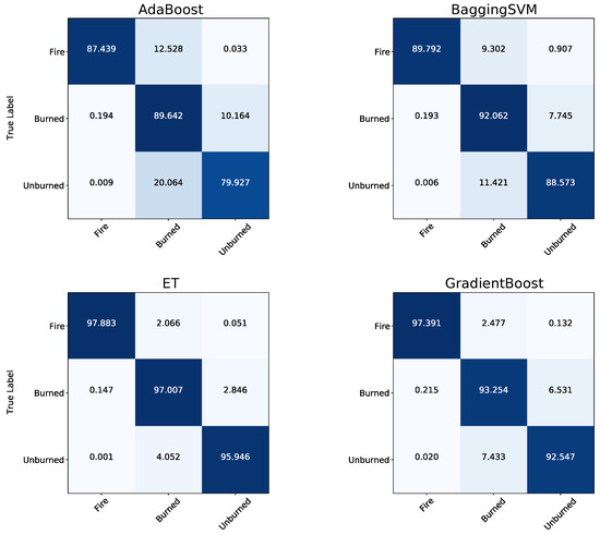

Figure A1.
Normalized confusion matrices for the investigated models. The prediction was performed on the unbalanced Subset 2 and compared to the reference data. The ML models were trained on the training split of Subset 3.
Figure A1.
Normalized confusion matrices for the investigated models. The prediction was performed on the unbalanced Subset 2 and compared to the reference data. The ML models were trained on the training split of Subset 3.
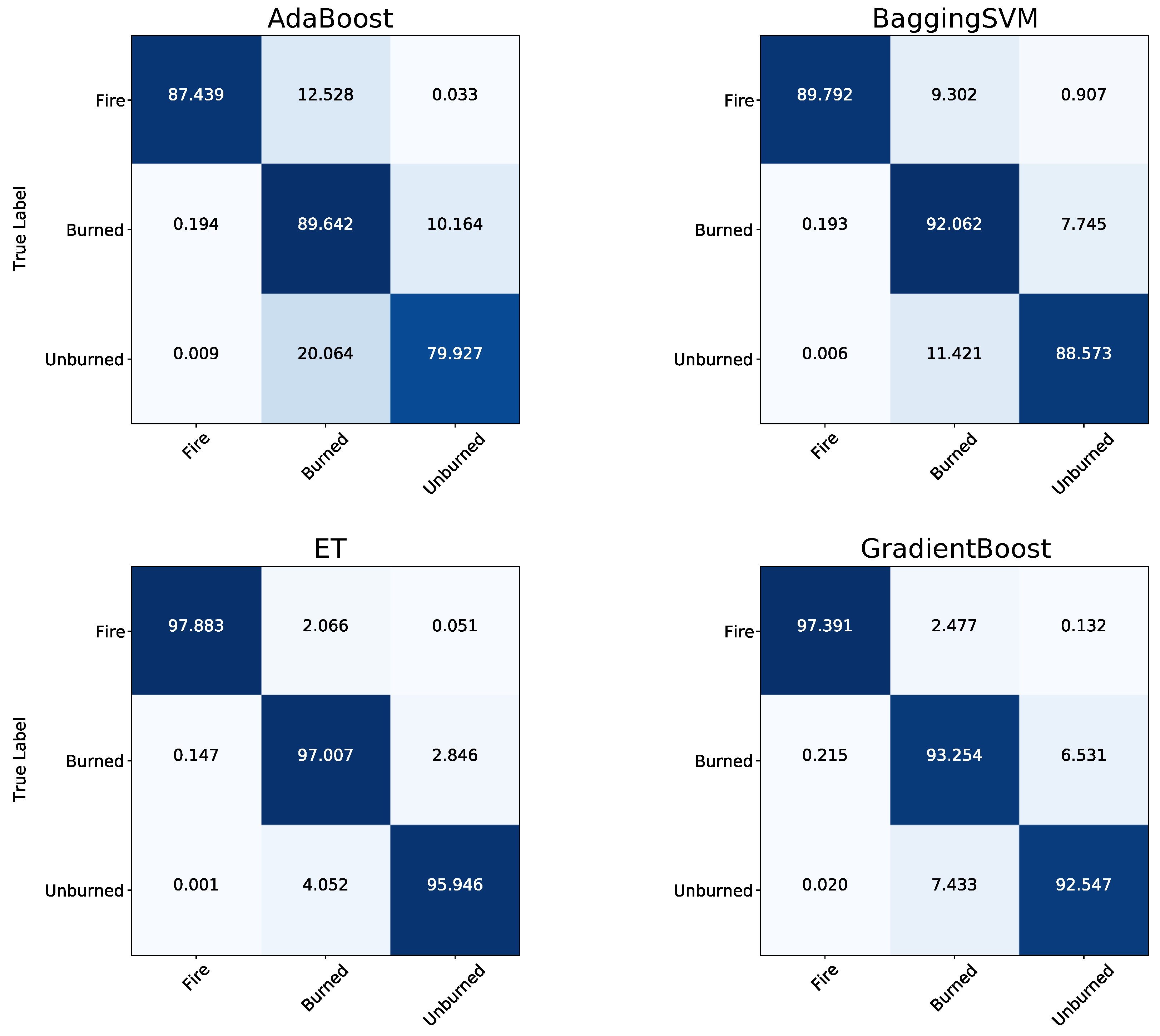
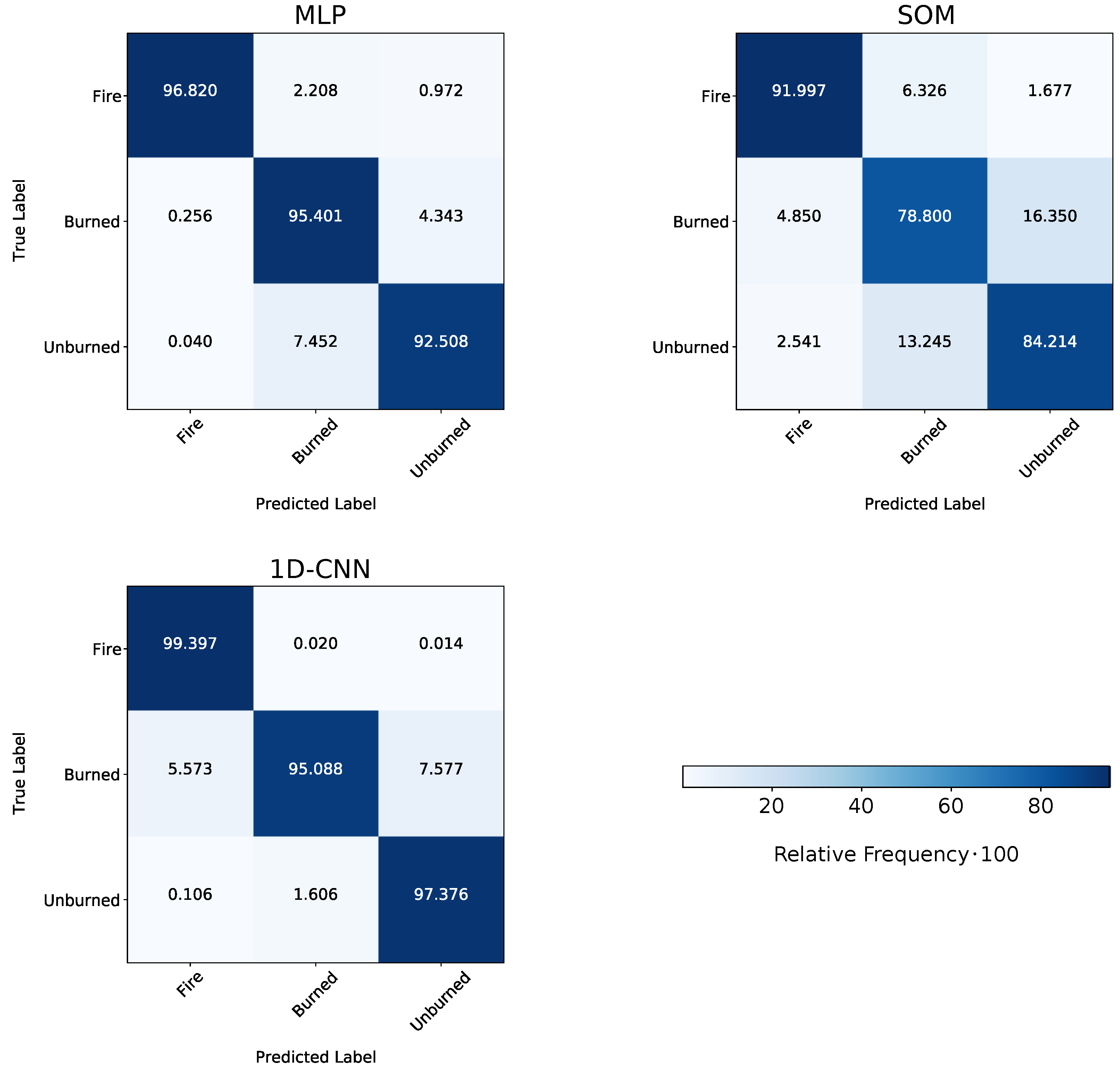
References
- Sharples, J.J.; Cary, G.J.; Fox-Hughes, P.; Mooney, S.; Evans, J.P.; Fletcher, M.S.; Fromm, M.; Grierson, P.F.; McRae, R.; Baker, P. Natural hazards in Australia: Extreme bushfire. Clim. Chang. 2016, 139, 85–99. [Google Scholar] [CrossRef]
- Boer, M.M.; de Dios, V.R.; Bradstock, R.A. Unprecedented burn area of Australian mega forest fires. Nat. Clim. Chang. 2020, 10, 171–172. [Google Scholar] [CrossRef]
- Lentile, L.B.; Holden, Z.A.; Smith, A.M.; Falkowski, M.J.; Hudak, A.T.; Morgan, P.; Lewis, S.A.; Gessler, P.E.; Benson, N.C. Remote sensing techniques to assess active fire characteristics and post-fire effects. Int. J. Wildland Fire 2006, 15, 319–345. [Google Scholar] [CrossRef]
- Bowman, D.M.; Balch, J.K.; Artaxo, P.; Bond, W.J.; Carlson, J.M.; Cochrane, M.A.; D’Antonio, C.M.; DeFries, R.S.; Doyle, J.C.; Harrison, S.P.; et al. Fire in the Earth system. Science 2009, 324, 481–484. [Google Scholar] [CrossRef] [PubMed]
- Filipponi, F. Exploitation of sentinel-2 time series to map burned areas at the national level: A case study on the 2017 Italy wildfires. Remote Sens. 2019, 11, 622. [Google Scholar] [CrossRef] [Green Version]
- Ghaffarian, S.; Kerle, N.; Pasolli, E.; Jokar Arsanjani, J. Post-disaster building database updating using automated deep learning: An integration of pre-disaster OpenStreetMap and multi-temporal satellite data. Remote Sens. 2019, 11, 2427. [Google Scholar] [CrossRef] [Green Version]
- Guth, J.; Wursthorn, S.; Braun, A.C.; Keller, S. Development of a generic concept to analyze the accessibility of emergency facilities in critical road infrastructure for disaster scenarios: Exemplary application for the 2017 wildfires in Chile and Portugal. Nat. Hazards 2019, 97, 979–999. [Google Scholar] [CrossRef]
- Henry, M.C.; Maingi, J.K.; McCarty, J. Fire on the Water Towers: Mapping Burn Scars on Mount Kenya Using Satellite Data to Reconstruct Recent Fire History. Remote Sens. 2019, 11, 104. [Google Scholar] [CrossRef] [Green Version]
- Guindos-Rojas, F.; Arbelo, M.; García-Lázaro, J.R.; Moreno-Ruiz, J.A.; Hernández-Leal, P.A. Evaluation of a Bayesian algorithm to detect Burned Areas in the Canary Islands’ Dry Woodlands and forests ecoregion using MODIS data. Remote Sens. 2018, 10, 789. [Google Scholar] [CrossRef] [Green Version]
- Schroeder, W.; Oliva, P.; Giglio, L.; Quayle, B.; Lorenz, E.; Morelli, F. Active fire detection using Landsat-8/OLI data. Remote Sens. Environ. 2016, 185, 210–220. [Google Scholar] [CrossRef] [Green Version]
- Giglio, L.; Csiszar, I.; Restás, Á.; Morisette, J.T.; Schroeder, W.; Morton, D.; Justice, C.O. Active fire detection and characterization with the advanced spaceborne thermal emission and reflection radiometer (ASTER). Remote Sens. Environ. 2008, 112, 3055–3063. [Google Scholar] [CrossRef]
- Crowley, M.A.; Cardille, J.A.; White, J.C.; Wulder, M.A. Multi-sensor, multi-scale, Bayesian data synthesis for mapping within-year wildfire progression. Remote Sens. Lett. 2019, 10, 302–311. [Google Scholar] [CrossRef]
- Chiaraviglio, N.; Artés, T.; Bocca, R.; López, J.; Gentile, A.; Ayanz, J.S.M.; Cortés, A.; Margalef, T. Automatic fire perimeter determination using MODIS hotspots information. In Proceedings of the 2016 IEEE 12th International Conference on e-Science (e-Science), Baltimore, MD, USA, 23–27 October 2016; pp. 414–423. [Google Scholar]
- Pereira, A.A.; Pereira, J.; Libonati, R.; Oom, D.; Setzer, A.W.; Morelli, F.; Machado-Silva, F.; De Carvalho, L.M.T. Burned area mapping in the Brazilian Savanna using a one-class support vector machine trained by active fires. Remote Sens. 2017, 9, 1161. [Google Scholar] [CrossRef] [Green Version]
- Cicala, L.; Angelino, C.V.; Fiscante, N.; Ullo, S.L. Landsat-8 and Sentinel-2 for fire monitoring at a local scale: A case study on Vesuvius. In Proceedings of the 2018 IEEE International Conference on Environmental Engineering (EE), Milan, Italy, 12–14 March 2018; pp. 1–6. [Google Scholar]
- Schroeder, W.; Oliva, P.; Giglio, L.; Csiszar, I.A. The New VIIRS 375 m active fire detection data product: Algorithm description and initial assessment. Remote Sens. Environ. 2014, 143, 85–96. [Google Scholar] [CrossRef]
- Gargiulo, M.; Dell’Aglio, D.A.G.; Iodice, A.; Riccio, D.; Ruello, G. A CNN-Based Super-Resolution Technique for Active Fire Detection on Sentinel-2 Data. In Proceedings of the 2019 PhotonIcs & Electromagnetics Research Symposium-Spring (PIERS-Spring), Rome, Italy, 17–20 June 2019; pp. 418–426. [Google Scholar]
- Oliva, P.; Schroeder, W. Assessment of VIIRS 375 m active fire detection product for direct burned area mapping. Remote Sens. Environ. 2015, 160, 144–155. [Google Scholar] [CrossRef]
- Stroppiana, D.; Pinnock, S.; Pereira, J.M.; Grégoire, J.M. Radiometric analysis of SPOT-VEGETATION images for burnt area detection in Northern Australia. Remote Sens. Environ. 2002, 82, 21–37. [Google Scholar] [CrossRef]
- Thomas, P.J.; Hersom, C.H.; Kourtz, P.; Buttner, G.J. Space-based forest fire detection concept. In Infrared Spaceborne Remote Sensing III; International Society for Optics and Photonics: Bellingham, WA, USA, 1995; Volume 2553, pp. 104–115. [Google Scholar]
- Giglio, L.; Descloitres, J.; Justice, C.O.; Kaufman, Y.J. An enhanced contextual fire detection algorithm for MODIS. Remote Sens. Environ. 2003, 87, 273–282. [Google Scholar] [CrossRef]
- NASA. MODIS Specifications; NASA: Washington, DC, USA, 2021. [Google Scholar]
- Kumar, S.S.; Roy, D.P. Global operational land imager Landsat-8 reflectance-based active fire detection algorithm. Int. J. Digit. Earth 2018, 11, 154–178. [Google Scholar] [CrossRef] [Green Version]
- Schroeder, W.; Prins, E.; Giglio, L.; Csiszar, I.; Schmidt, C.; Morisette, J.; Morton, D. Validation of GOES and MODIS active fire detection products using ASTER and ETM+ data. Remote Sens. Environ. 2008, 112, 2711–2726. [Google Scholar] [CrossRef]
- Engelbrecht, J.; Theron, A.; Vhengani, L.; Kemp, J. A simple normalized difference approach to burnt area mapping using multi-polarisation C-Band SAR. Remote Sens. 2017, 9, 764. [Google Scholar] [CrossRef] [Green Version]
- Siegert, F.; Hoffmann, A.A. The 1998 forest fires in East Kalimantan (Indonesia): A quantitative evaluation using high resolution, multitemporal ERS-2 SAR images and NOAA-AVHRR hotspot data. Remote Sens. Environ. 2000, 72, 64–77. [Google Scholar] [CrossRef]
- Axel, A.C. Burned area mapping of an escaped fire into tropical dry forest in Western Madagascar using multi-season Landsat OLI Data. Remote Sens. 2018, 10, 371. [Google Scholar] [CrossRef] [Green Version]
- Polychronaki, A.; Gitas, I.Z. The development of an operational procedure for burned-area mapping using object-based classification and ASTER imagery. Int. J. Remote Sens. 2010, 31, 1113–1120. [Google Scholar] [CrossRef]
- Gitas, I.Z.; Mitri, G.H.; Ventura, G. Object-based image classification for burned area mapping of Creus Cape, Spain, using NOAA-AVHRR imagery. Remote Sens. Environ. 2004, 92, 409–413. [Google Scholar] [CrossRef]
- Grivei, A.C.; Văduva, C.; Datcu, M. Assessment of Burned Area Mapping Methods for Smoke Covered Sentinel-2 Data. In Proceedings of the 2020 13th International Conference on Communications (COMM), Bucharest, Romania, 18–20 June 2020; pp. 189–192. [Google Scholar]
- Knopp, L.; Wieland, M.; Rättich, M.; Martinis, S. A Deep Learning Approach for Burned Area Segmentation with Sentinel-2 Data. Remote Sens. 2020, 12, 2422. [Google Scholar] [CrossRef]
- Rashkovetsky, D.; Mauracher, F.; Langer, M.; Schmitt, M. Wildfire Detection from Multi-sensor Satellite Imagery Using Deep Semantic Segmentation. IEEE J. Sel. Top. Appl. Earth Obs. Remote Sens. 2021, 14, 7001–7016. [Google Scholar] [CrossRef]
- Rauste, Y.; Herland, E.; Frelander, H.; Soini, K.; Kuoremaki, T.; Ruokari, A. Satellite-based forest fire detection for fire control in boreal forests. Int. J. Remote Sens. 1997, 18, 2641–2656. [Google Scholar] [CrossRef]
- Matson, M.; Stephens, G.; Robinson, J. Fire detection using data from the NOAA-N satellites. Int. J. Remote Sens. 1987, 8, 961–970. [Google Scholar] [CrossRef]
- Xie, Z.; Song, W.; Ba, R.; Li, X.; Xia, L. A spatiotemporal contextual model for forest fire detection using Himawari-8 satellite data. Remote Sens. 2018, 10, 1992. [Google Scholar] [CrossRef] [Green Version]
- Flasse, S.; Ceccato, P. A contextual algorithm for AVHRR fire detection. Int. J. Remote Sens. 1996, 17, 419–424. [Google Scholar] [CrossRef]
- Giglio, L.; Schroeder, W.; Justice, C.O. The collection 6 MODIS active fire detection algorithm and fire products. Remote Sens. Environ. 2016, 178, 31–41. [Google Scholar] [CrossRef] [PubMed] [Green Version]
- Di Biase, V.; Laneve, G. Geostationary sensor based forest fire detection and monitoring: An improved version of the SFIDE algorithm. Remote Sens. 2018, 10, 741. [Google Scholar] [CrossRef] [Green Version]
- San-Miguel-Ayanz, J.; Ravail, N. Active fire detection for fire emergency management: Potential and limitations for the operational use of remote sensing. Nat. Hazards 2005, 35, 361–376. [Google Scholar] [CrossRef] [Green Version]
- Koltunov, A.; Ustin, S.L.; Quayle, B.; Schwind, B.; Ambrosia, V.G.; Li, W. The development and first validation of the GOES Early Fire Detection (GOES-EFD) algorithm. Remote Sens. Environ. 2016, 184, 436–453. [Google Scholar] [CrossRef] [Green Version]
- Kurum, M. C-band SAR backscatter evaluation of 2008 Gallipoli forest fire. IEEE Geosci. Remote Sens. Lett. 2015, 12, 1091–1095. [Google Scholar] [CrossRef]
- Ruecker, G.; Siegert, F. Burn scar mapping and fire damage assessment using ERS-2 Sar images in East Kalimantan, Indonesia. Int. Arch. Photogramm. Remote Sens. 2000, 33, 1286–1293. [Google Scholar]
- Goodenough, D.G.; Chen, H.; Richardson, A.; Cloude, S.; Hong, W.; Li, Y. Mapping fire scars using Radarsat-2 polarimetric SAR data. Can. J. Remote Sens. 2011, 37, 500–509. [Google Scholar] [CrossRef] [Green Version]
- Wei, J.; Zhang, Y.; Wu, H.; Cui, B. The Automatic Detection of Fire Scar in Alaska using Multi-Temporal PALSAR Polarimetric SAR Data. Can. J. Remote Sens. 2018, 44, 447–461. [Google Scholar] [CrossRef]
- Ban, Y.; Zhang, P.; Nascetti, A.; Bevington, A.R.; Wulder, M.A. Near real-time wildfire progression monitoring with Sentinel-1 SAR time series and deep learning. Sci. Rep. 2020, 10, 1–15. [Google Scholar] [CrossRef] [Green Version]
- Mithal, V.; Nayak, G.; Khandelwal, A.; Kumar, V.; Nemani, R.; Oza, N.C. Mapping burned areas in tropical forests using a novel machine learning framework. Remote Sens. 2018, 10, 69. [Google Scholar] [CrossRef] [Green Version]
- Libonati, R.; DaCamara, C.C.; Setzer, A.W.; Morelli, F.; Melchiori, A.E. An algorithm for burned area detection in the Brazilian Cerrado using 4 μm MODIS imagery. Remote Rens. 2015, 7, 15782–15803. [Google Scholar]
- Bastarrika, A.; Alvarado, M.; Artano, K.; Martinez, M.P.; Mesanza, A.; Torre, L.; Ramo, R.; Chuvieco, E. BAMS: A tool for supervised burned area mapping using Landsat data. Remote Sens. 2014, 6, 12360–12380. [Google Scholar] [CrossRef] [Green Version]
- Stroppiana, D.; Bordogna, G.; Carrara, P.; Boschetti, M.; Boschetti, L.; Brivio, P.A. A method for extracting burned areas from Landsat TM/ETM+ images by soft aggregation of multiple Spectral Indices and a region growing algorithm. ISPRS J. Photogramm. Remote Sens. 2012, 69, 88–102. [Google Scholar] [CrossRef]
- Kurnaz, B.; Bayik, C.; Abdikan, S. Forest Fire Area Detection by Using Landsat-8 and Sentinel-2 Satellite Images: A Case Study in Mugla, Turkey; Research Square: Ankara, Turkey, 2020. [Google Scholar]
- Bastarrika, A.; Chuvieco, E.; Martin, P.M. Mapping burned areas from Landsat TM/ETM+ data with a two-phase algorithm: Balancing omission and commission errors. Remote Sens. Environ. 2011, 115, 1003–1012. [Google Scholar] [CrossRef]
- Bastarrika, A.; Barrett, B.; Roteta, E.; Akizu, O.; Mesanza, A.; Torre, L.; Anaya, J.A.; Rodriguez-Montellano, A.; Chuvieco, E. Mapping burned areas in Latin America from Landsat-8 with Google Earth Engine. Remote Sens. 2018. [Google Scholar] [CrossRef]
- Ramo, R.; Chuvieco, E. Developing a random forest algorithm for MODIS global burned area classification. Remote Sens. 2017, 9, 1193. [Google Scholar] [CrossRef] [Green Version]
- Mitri, G.H.; Gitas, I.Z. The development of an object-oriented classification model for operational burned area mapping on the Mediterranean island of Thasos using LANDSAT TM images. In Forest Fire Research & Wildland Fire Safety; Millpress: Bethlehem, PA, USA, 2002; pp. 1–12. [Google Scholar]
- Çömert, R.; Matci, D.K.; Avdan, U. Object Based Burned Area Mapping with Random Forest Algorithm. Int. J. Eng. Geosci. 2019, 4, 78–87. [Google Scholar] [CrossRef]
- Mallinis, G.; Koutsias, N. Comparing ten classification methods for burned area mapping in a Mediterranean environment using Landsat TM satellite data. Int. J. Remote Sens. 2012, 33, 4408–4433. [Google Scholar] [CrossRef]
- Pereira, M.C.; Setzer, A.W. Spectral characteristics of fire scars in Landsat-5 TM images of Amazonia. Remote Sens. 1993, 14, 2061–2078. [Google Scholar] [CrossRef]
- Mitrakis, N.E.; Mallinis, G.; Koutsias, N.; Theocharis, J.B. Burned area mapping in Mediterranean environment using medium-resolution multi-spectral data and a neuro-fuzzy classifier. Int. J. Image Data Fusion 2012, 3, 299–318. [Google Scholar] [CrossRef]
- Brand, A.; Manandhar, A. Semantic Segmentation of Burned Areas in Satellite Images Using a U-Net Convolutional Neural Network. ISPRS-Int. Arch. Photogramm. Remote Sens. Spat. Inf. Sci. 2021, 43, 47–53. [Google Scholar] [CrossRef]
- Barducci, A.; Guzzi, D.; Marcoionni, P.; Pippi, I. Infrared detection of active fires and burnt areas: Theory and observations. Infrared Phys. Technol. 2002, 43, 119–125. [Google Scholar] [CrossRef]
- Calle, A.; Casanova, J.; Romo, A. Fire detection and monitoring using MSG Spinning Enhanced Visible and Infrared Imager (SEVIRI) data. J. Geophys. Res. Biogeosci. 2006, 111. [Google Scholar] [CrossRef]
- Michael, Y.; Lensky, I.M.; Brenner, S.; Tchetchik, A.; Tessler, N.; Helman, D. Economic assessment of fire damage to urban forest in the wildland–urban interface using planet satellites constellation images. Remote Sens. 2018, 10, 1479. [Google Scholar] [CrossRef] [Green Version]
- Riese, F.M.; Keller, S. Supervised, Semi-Supervised, and Unsupervised Learning for Hyperspectral Regression. In Hyperspectral Image Analysis; Springer: Cham, Switzerland, 2020; pp. 187–232. [Google Scholar]
- State of California CAL FIRE. Available online: https://frap.fire.ca.gov/mapping/gis-data/ (accessed on 13 January 2022).
- Buchhorn, M.; Lesiv, M.; Tsendbazar, N.E.; Herold, M.; Bertels, L.; Smets, B. Copernicus Global Land Cover Layers—Collection 2. Remote Sens. 2020, 12, 1044. [Google Scholar] [CrossRef] [Green Version]
- Wu, Q. geemap: A Python package for interactive mapping with Google Earth Engine. J. Open Source Softw. 2020, 5, 2305. [Google Scholar] [CrossRef]
- Weiss, G.M. Foundations of imbalanced learning. In Imbalanced Learning: Foundations, Algorithms, and Applications; Wiley: Hoboken, NJ, USA, 2013; pp. 13–41. [Google Scholar]
- Chawla, N.V.; Japkowicz, N.; Kotcz, A. Special issue on learning from imbalanced data sets. ACM SIGKDD Explor. Newsl. 2004, 6, 1–6. [Google Scholar] [CrossRef]
- Liu, X.Y.; Wu, J.; Zhou, Z.H. Exploratory undersampling for class-imbalance learning. IEEE Trans. Syst. Man Cybern. Part B Cybern. 2008, 39, 539–550. [Google Scholar]
- Kattenborn, T.; Leitloff, J.; Schiefer, F.; Hinz, S. Review on Convolutional Neural Networks (CNN) in vegetation remote sensing. ISPRS J. Photogramm. Remote Sens. 2021, 173, 24–49. [Google Scholar] [CrossRef]
- Drummond, C.; Holte, R.C. C4. 5, class imbalance, and cost sensitivity: Why under-sampling beats over-sampling. In Workshop on Learning from Imbalanced Datasets II; Citeseer: Princeton, NJ, USA, 2003; Volume 11, pp. 1–8. [Google Scholar]
- Geurts, P.; Ernst, D.; Wehenkel, L. Extremely randomized trees. Mach. Learn. 2006, 63, 3–42. [Google Scholar] [CrossRef] [Green Version]
- Freund, Y.; Schapire, R.E. A decision-theoretic generalization of on-line learning and an application to boosting. J. Comput. Syst. Sci. 1997, 55, 119–139. [Google Scholar] [CrossRef] [Green Version]
- Friedman, J.H. Greedy function approximation: A gradient boosting machine. In Annals of Statistics; Institute of Mathematical Statistics: Shaker Heights, OH, USA, 2001; pp. 1189–1232. [Google Scholar]
- Hinton, G.E. Connectionist learning procedures. In Machine Learning; Elsevier: Amsterdam, The Netherlands, 1990; pp. 555–610. [Google Scholar]
- Riese, F.M.; Keller, S.; Hinz, S. Supervised and semi-supervised self-organizing maps for regression and classification focusing on hyperspectral data. Remote Sens. 2020, 12, 7. [Google Scholar] [CrossRef] [Green Version]
- Riese, F.M.; Keller, S. Introducing a framework of self-organizing maps for regression of soil moisture with hyperspectral data. In Proceedings of the IGARSS 2018-2018 IEEE International Geoscience and Remote Sensing Symposium, Valencia, Spain, 22–27 July 2018; pp. 6151–6154. [Google Scholar]
- Kohonen, T. The self-organizing map. Proc. IEEE 1990, 78, 1464–1480. [Google Scholar] [CrossRef]
- Kim, H.C.; Pang, S.; Je, H.M.; Kim, D.; Bang, S.Y. Support vector machine ensemble with bagging. In International Workshop on Support Vector Machines; Springer: Berlin, Germany, 2002; pp. 397–408. [Google Scholar]
- Riese, F.M.; Keller, S. Soil texture classification with 1D convolutional neural networks based on hyperspectral data. ISPRS Ann. Photogramm. Remote Sens. Spat. Inf. Sci. 2019, IV-2/W5, 615–621. [Google Scholar] [CrossRef] [Green Version]
- Hansen, M.C.; DeFries, R.S.; Townshend, J.R.; Sohlberg, R. Global land cover classification at 1 km spatial resolution using a classification tree approach. Int. J. Remote Sens. 2000, 21, 1331–1364. [Google Scholar] [CrossRef]
- Lasaponara, R.; Proto, M.; Aromando, A.; Cardettini, G.; Varela, V.; Danese, M. On the mapping of burned areas and burn severity using self organizing map and sentinel-2 data. IEEE Geosci. Remote Sens. Lett. 2019, 17, 854–858. [Google Scholar] [CrossRef]
- Riese, F.M. SuSi: Supervised Self-Organizing Maps in Python; Zenodo: Geneve, Switzerland, 2019. [Google Scholar] [CrossRef]
- Pedregosa, F.; Varoquaux, G.; Gramfort, A.; Michel, V.; Thirion, B.; Grisel, O.; Blondel, M.; Prettenhofer, P.; Weiss, R.; Dubourg, V.; et al. Scikit-learn: Machine Learning in Python. J. Mach. Learn. Res. 2011, 12, 2825–2830. [Google Scholar]
- Rosenblatt, F. The perceptron: A probabilistic model for information storage and organization in the brain. Psychol. Rev. 1958, 65, 386. [Google Scholar] [CrossRef] [Green Version]
- Liu, L.; Ji, M.; Buchroithner, M. Transfer learning for soil spectroscopy based on convolutional neural networks and its application in soil clay content mapping using hyperspectral imagery. Sensors 2018, 18, 3169. [Google Scholar] [CrossRef] [Green Version]
- Hu, W.; Huang, Y.; Wei, L.; Zhang, F.; Li, H. Deep convolutional neural networks for hyperspectral image classification. J. Sens. 2015, 2015, 258619. [Google Scholar] [CrossRef] [Green Version]
- Li, L.; Jamieson, K.; DeSalvo, G.; Rostamizadeh, A.; Talwalkar, A. Hyperband: A novel bandit-based approach to hyperparameter optimization. J. Mach. Learn. Res. 2017, 18, 6765–6816. [Google Scholar]
- Mosley, L. A Balanced Approach to the Multi-Class Imbalance Problem; Iowa State University: Ames, IA, USA, 2013. [Google Scholar]
- Cervone, G.; Sava, E.; Huang, Q.; Schnebele, E.; Harrison, J.; Waters, N. Using Twitter for tasking remote-sensing data collection and damage assessment: 2013 Boulder flood case study. Int. J. Remote Sens. 2016, 37, 100–124. [Google Scholar] [CrossRef]
- Bruneau, P.; Brangbour, E.; Marchand-Maillet, S.; Hostache, R.; Chini, M.; Pelich, R.M.; Matgen, P.; Tamisier, T. Measuring the Impact of Natural Hazards with Citizen Science: The Case of Flooded Area Estimation Using Twitter. Remote Sens. 2021, 13, 1153. [Google Scholar] [CrossRef]
- Kruspe, A.; Häberle, M.; Hoffmann, E.J.; Rode-Hasinger, S.; Abdulahhad, K.; Zhu, X.X. Changes in Twitter geolocations: Insights and suggestions for future usage. arXiv 2021, arXiv:2108.12251. [Google Scholar]
- Abadi, M.; Barham, P.; Chen, J.; Chen, Z.; Davis, A.; Dean, J.; Devin, M.; Ghemawat, S.; Irving, G.; Isard, M.; et al. Tensorflow: A system for large-scale machine learning. In Proceedings of the 12th Symposium on Operating Systems Design and Implementation, Savannah, GA, USA, 2–4 November 2016; pp. 265–283. [Google Scholar]
Publisher’s Note: MDPI stays neutral with regard to jurisdictional claims in published maps and institutional affiliations. |
© 2022 by the authors. Licensee MDPI, Basel, Switzerland. This article is an open access article distributed under the terms and conditions of the Creative Commons Attribution (CC BY) license (https://creativecommons.org/licenses/by/4.0/).

