
A Simple, Fully Automated Shoreline Detection Algorithm for High-Resolution Multi-Spectral Imagery


Abstract
:1. Introduction

| Index Name | Definition | Applicable Satellites | References |
|---|---|---|---|
| Normalized Difference Water Index | Landsat, Sentinel, Planetscope, RapidEye | [12,13,23] | |
| Normalized Difference Vegetation Index | Landsat, Sentinel, Planetscope, RapidEye | [24] | |
| Modified Normalized Difference Water Index | Landsat, Sentinel | [14,15] | |
| Coastal Water Index | Landsat | [25] | |
| Tasseled Cap Wetness | Landsat | [13] | |
| Coal Mine Index | Landsat | [12] | |
| Automated Water Extraction Index | Landsat | [19,20] |
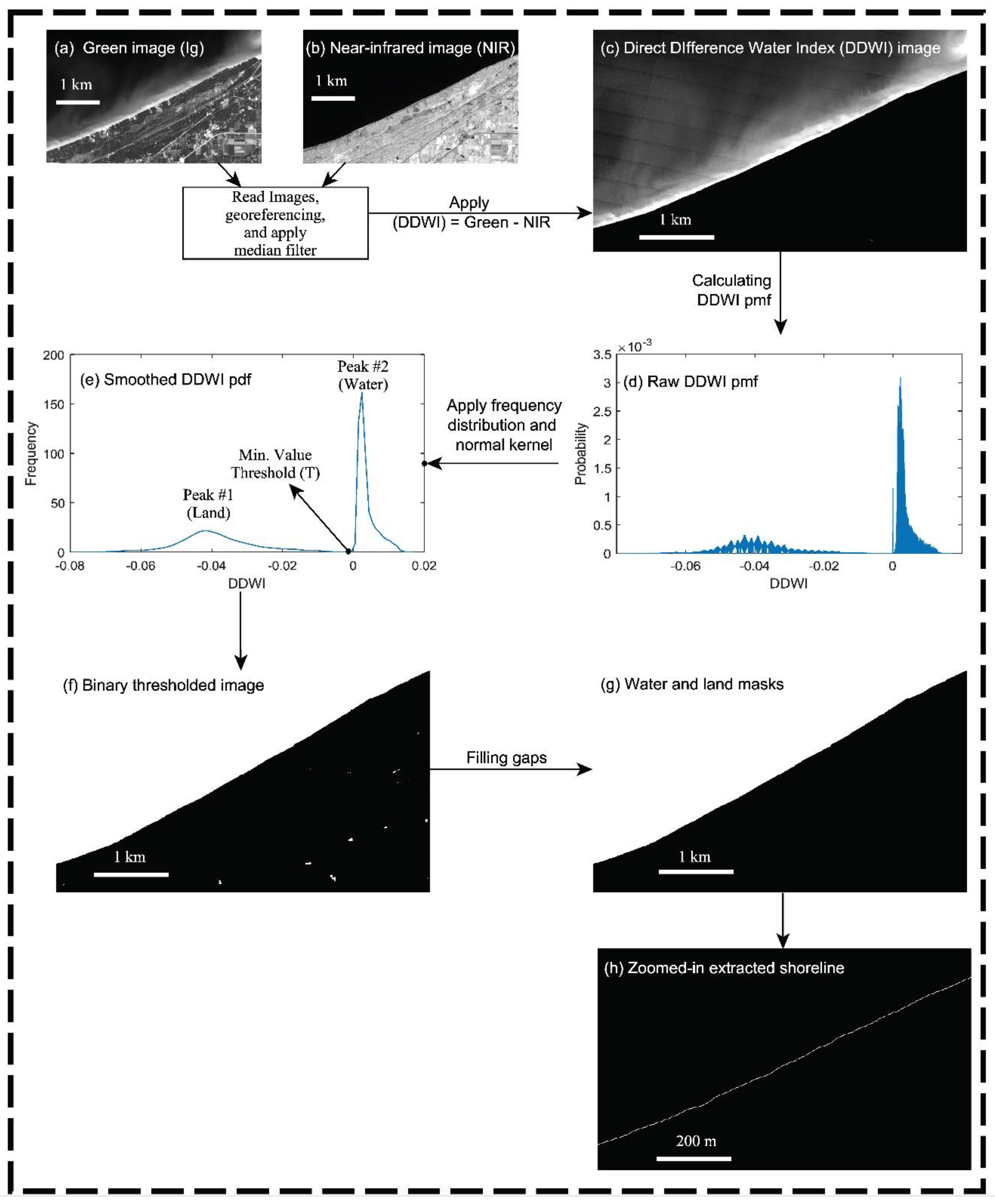
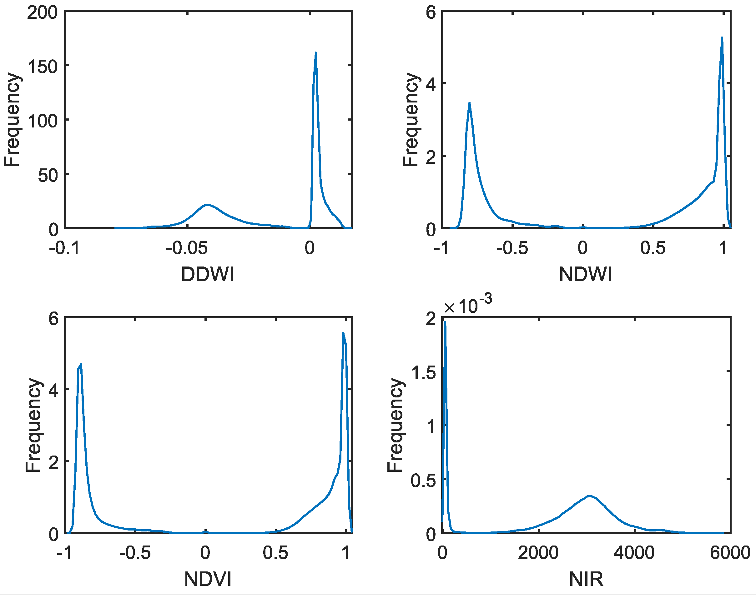
2. Improved Procedure for Fully Automated Shoreline Detection from Multispectral Imagery
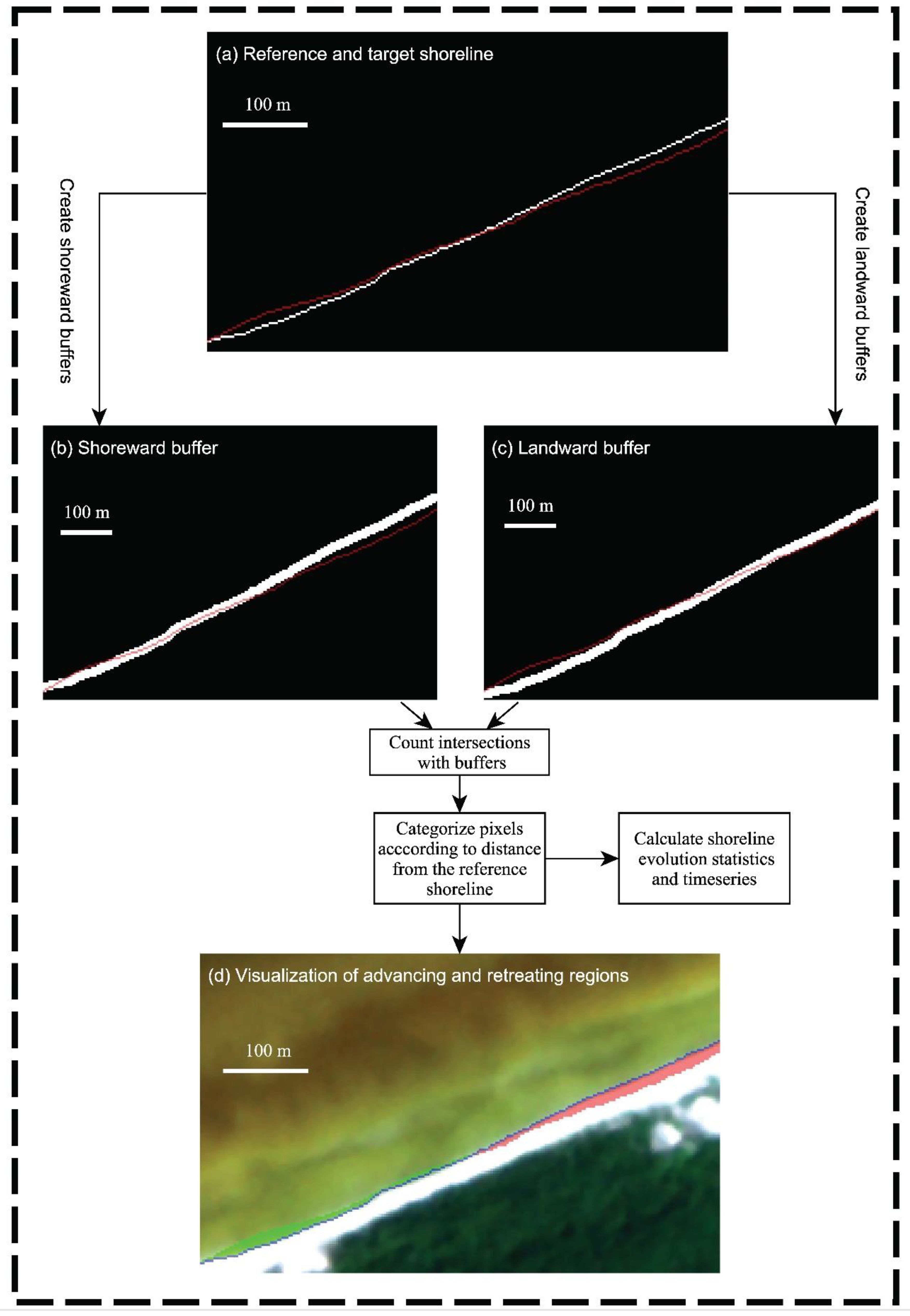
Shoreline Movement Quantification
3. Methods
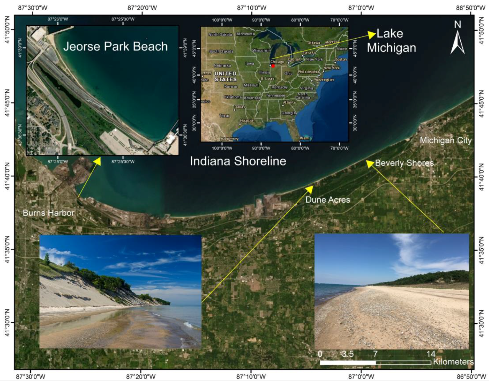
3.1. Study Areas
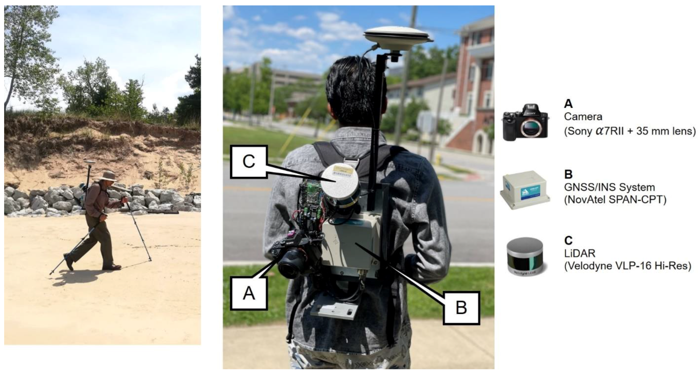
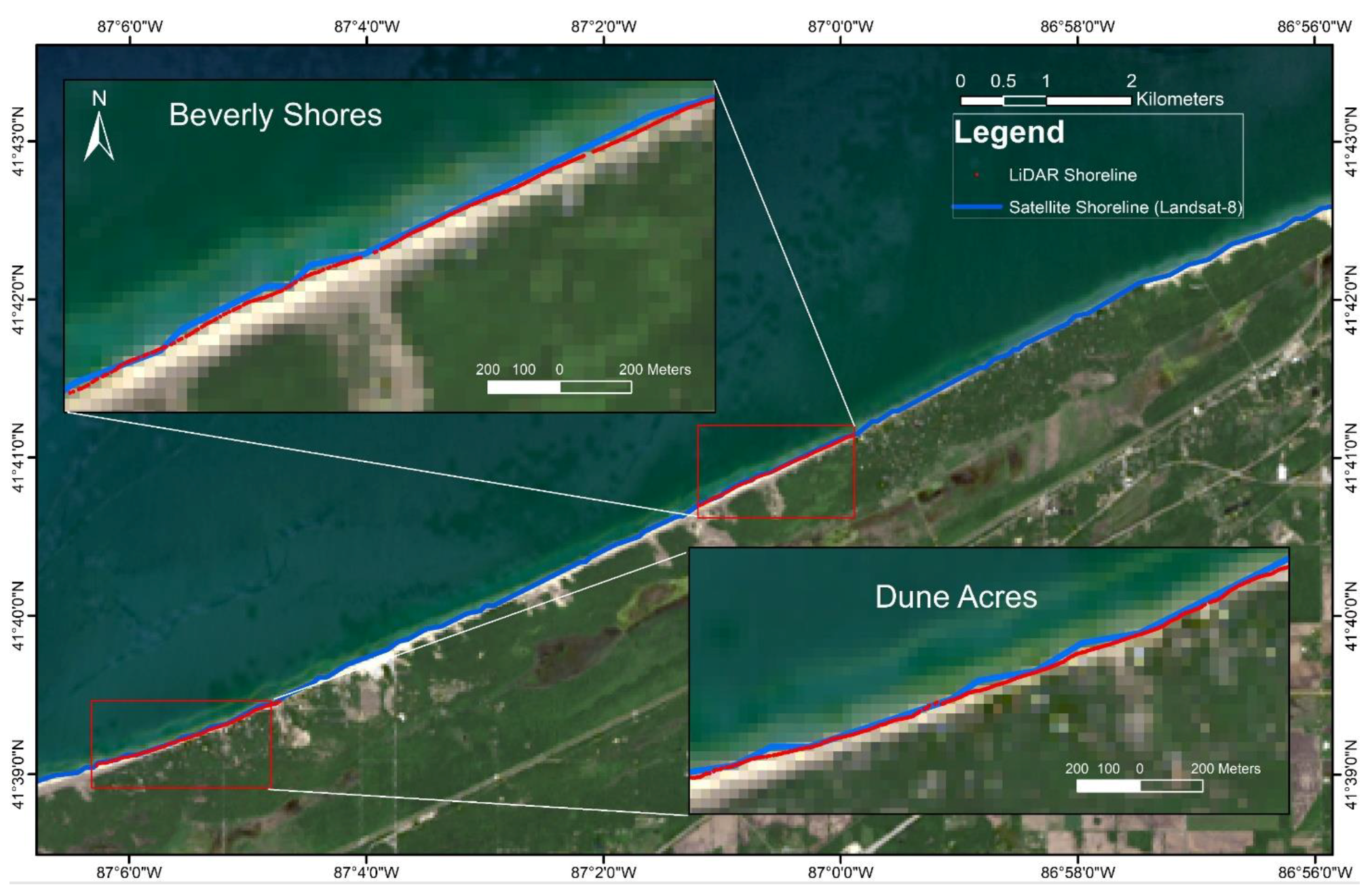
3.2. LiDAR Shoreline Surveys
3.3. Satellite Imagery
3.4. Test 1—Comparison with LiDAR Surveys
3.5. Test 2—Comparison with Other Shoreline Detection Algorithms
4. Results
4.1. Validation of Shoreline Detection Algorithm
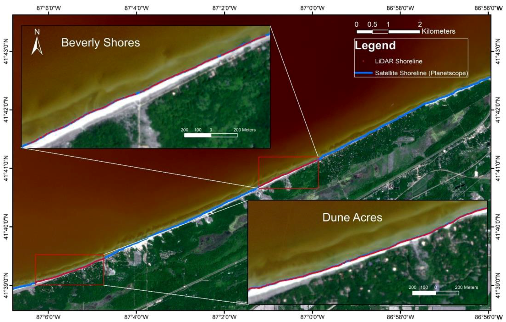
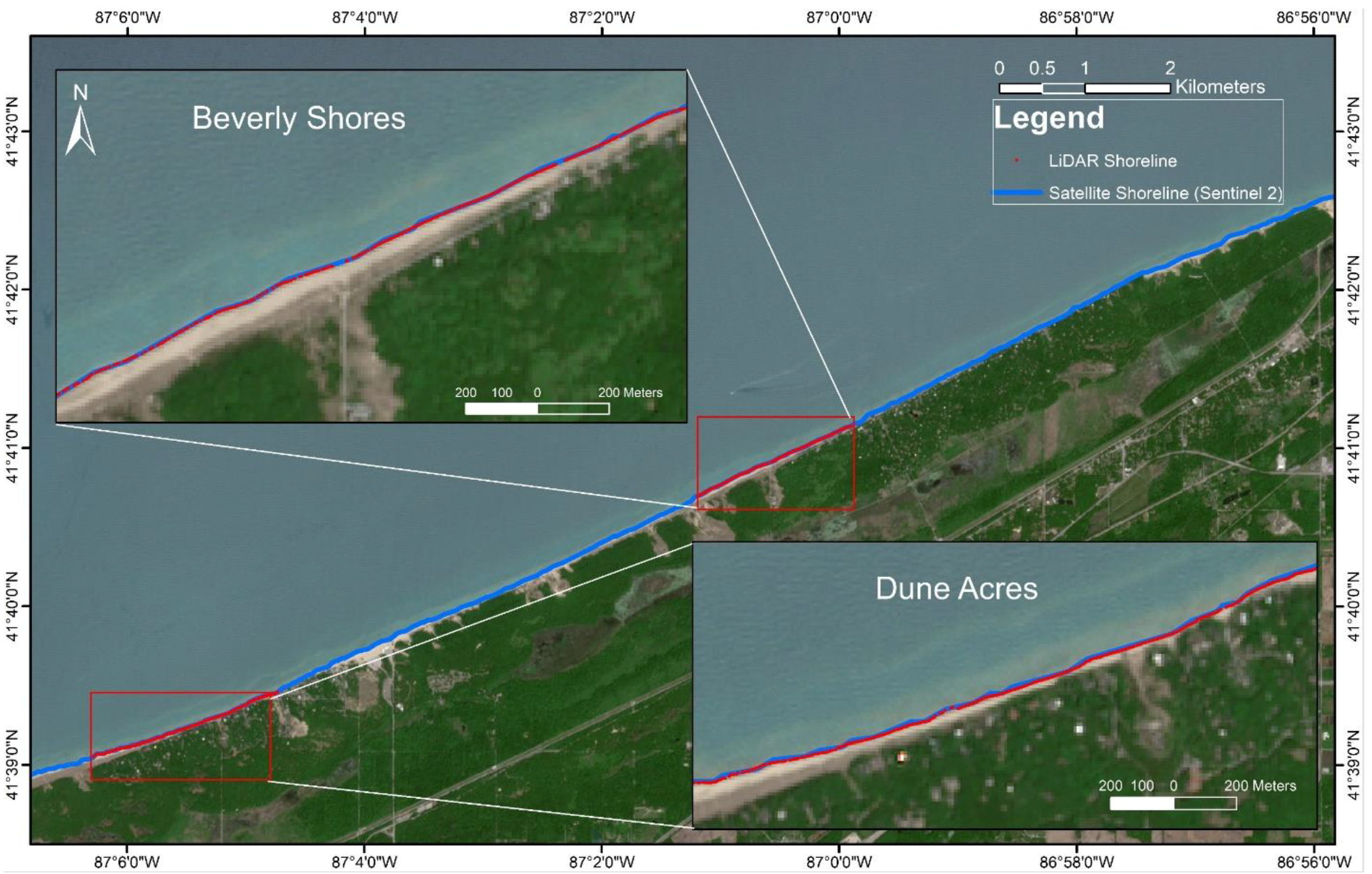
4.1.1. Test 1—Comparison with LiDAR Surveys
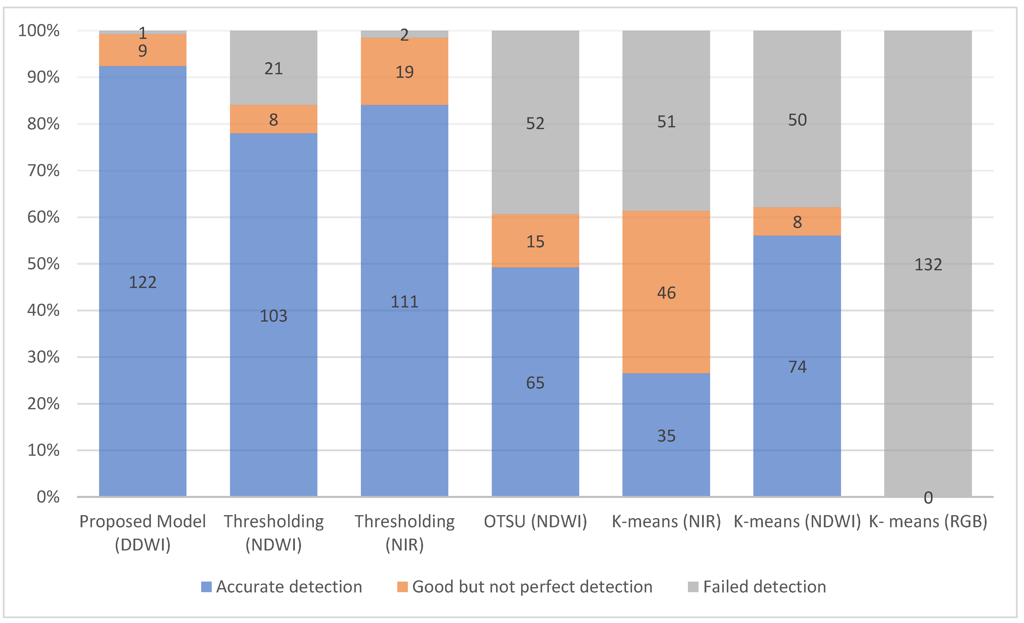
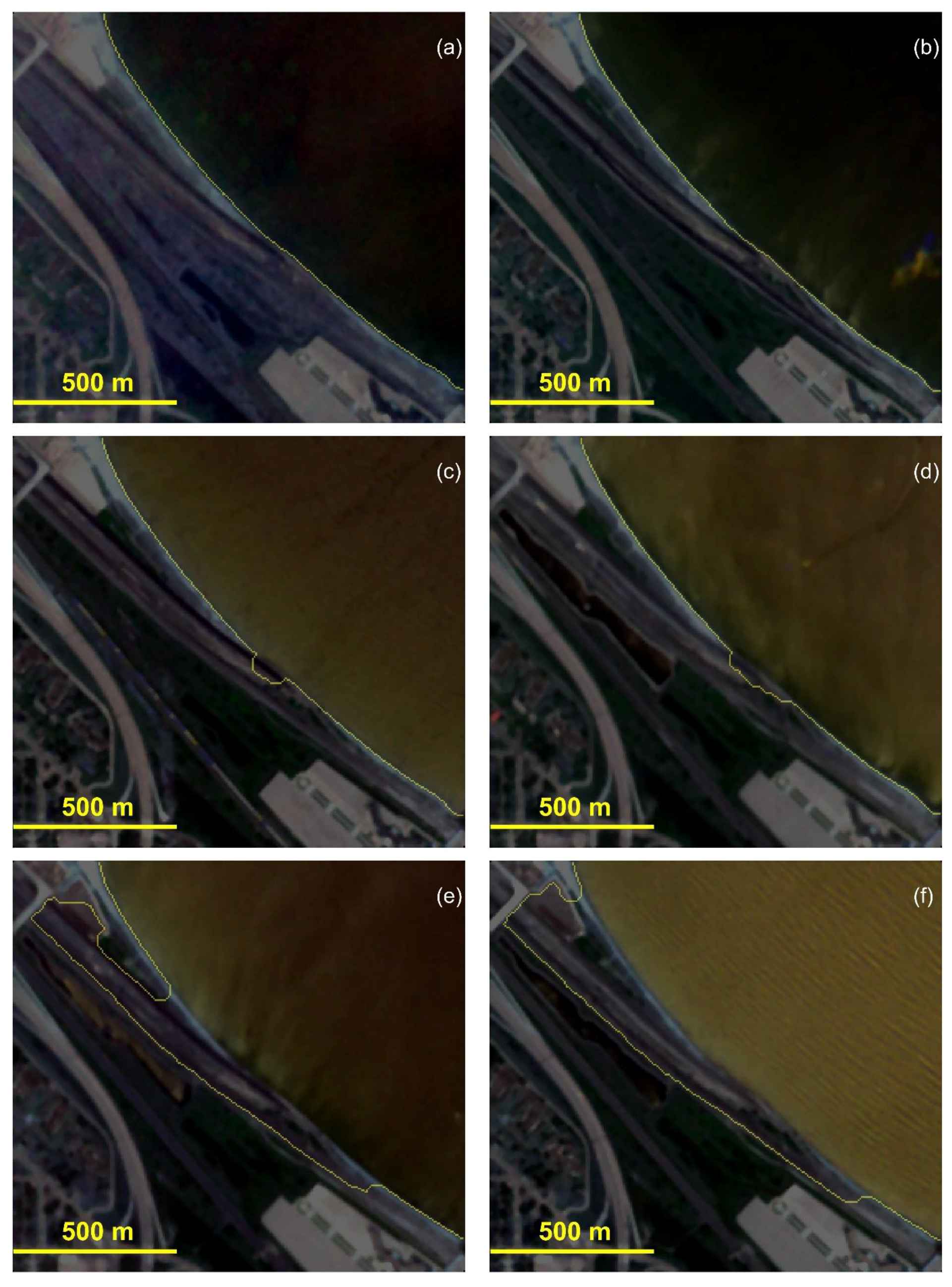
4.1.2. Test 2—Comparison with Other Shoreline Detection Methods
4.2. Shoreline Evolution Module Results
5. Discussion
- Using LiDAR, it is possible to delineate the actual shoreline (land–water intersection). In areas where a clear distinction cannot be established, imagery can be used to verify the ground condition.
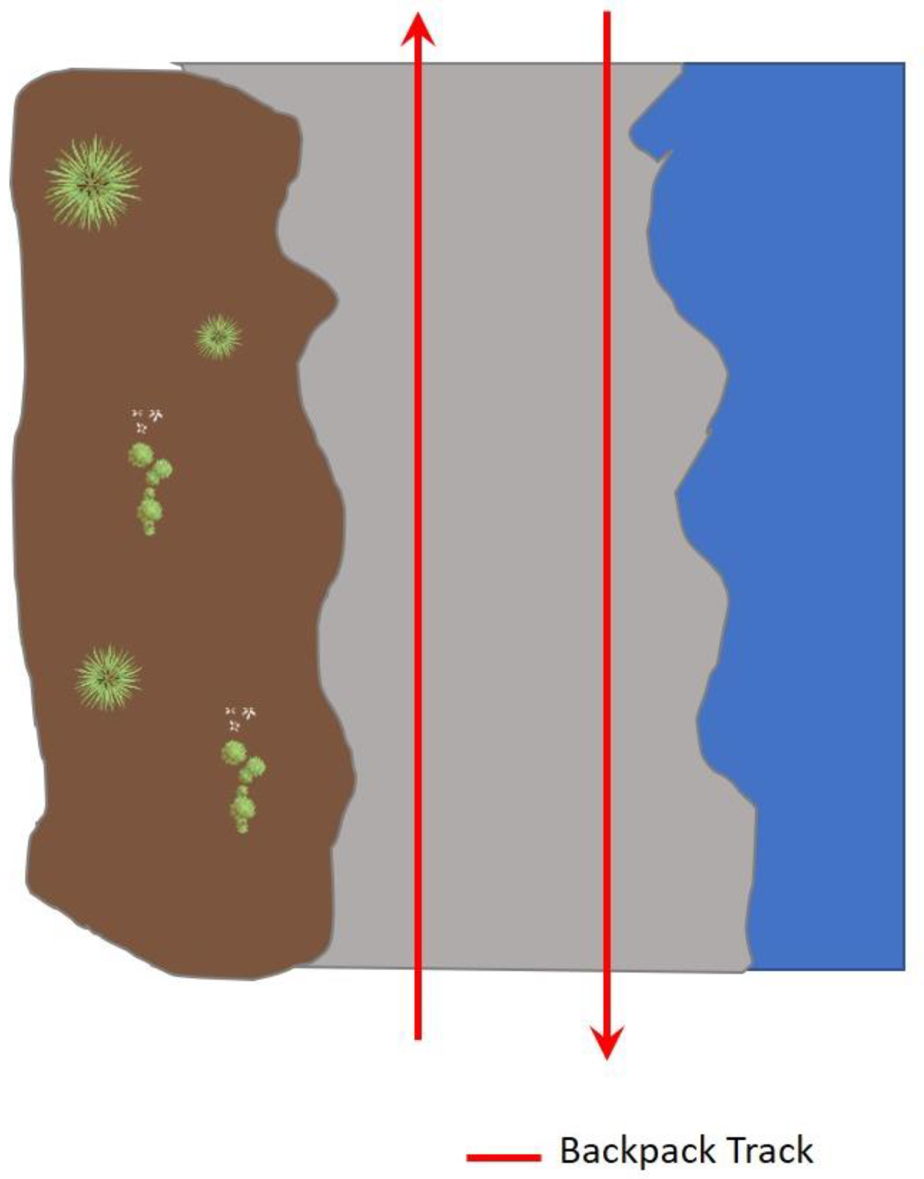
- The point density of a Backpack-based LiDAR is very high compared to UAV-based point clouds due to the proximity of the former to the surface. However, this comes at the price of an increased data acquisition time in the case of the Backpack system.
- The use of a Backpack-based LiDAR system may not require extensive regulatory approval, unlike vehicle-based or unmanned aerial platforms (as in Indiana dunes). More specifically, the Backpack system can be used regardless of the nature/restrictions of the airspace at the vicinity of shorelines.
- Unlike UAVs, Backpack-based LiDAR can be used in less favorable weather conditions. Additionally, it does not have any requirements for a clear takeoff/landing site, as in the case of UAV systems.
6. Conclusions
Author Contributions
Funding
Institutional Review Board Statement
Informed Consent Statement
Data Availability Statement
Acknowledgments
Conflicts of Interest
References
- Small, C.; Nicholls, R.J. A global analysis of human settlement in coastal zones. J. Coast. Res. 2003, 19, 584–599. [Google Scholar]
- Brown, S.; Nicholls, R.J.; Woodroffe, C.D.; Hanson, S.; Hinkel, J.; Kebede, A.S.; Neumann, B.; Vafeidis, A.T. Sea-Level Rise Impacts and Responses: A Global Perspective, Coastal Research Library. In Coastal Hazards; Springer: Dordrecht, The Netherland, 2013; pp. 117–149. [Google Scholar] [CrossRef]
- Neumann, B.; Vafeidis, A.T.; Zimmermann, J.; Nicholls, R.J. Future Coastal Population Growth and Exposure to Sea-Level Rise and Coastal Flooding—A Global Assessment. PLoS ONE 2015, 10, e0118571. [Google Scholar] [CrossRef] [PubMed] [Green Version]
- Baily, B.; Nowell, D. Techniques for monitoring coastal change: A review and case study. Ocean. Coast. Manag. 1996, 32, 85–95. [Google Scholar] [CrossRef]
- Eulie, D.O.; Corbett, D.R.; Walsh, J.P. Shoreline erosion and decadal sediment accumulation in the Tar-Pamlico estuary, North Carolina, USA: A source-to-sink analysis. Estuar. Coast. Shelf Sci. 2018, 202, 246–258. [Google Scholar] [CrossRef]
- Reif, M.K.; Wozencraft, J.M.; Dunkin, L.M.; Sylvester, C.S.; Macon, C.L. A review of U.S. Army Corps of Engineers airborne coastal mapping in the Great Lakes. J. Great Lakes Res. 2013, 39, 194–204. [Google Scholar] [CrossRef]
- Feygels, V.I.; Park, J.Y.; Wozencraft, J.; Aitken, J.; Macon, C.; Mathur, A.; Payment, A.; Ramnath, V.; Feygels, V.I. CZMIL (coastal zone mapping and imaging lidar): From first flights to first mission through system validation. In Ocean Sensing and Monitoring V, Proceeding of the International Society for Optics and Photonics, Baltimore, MD, USA, 29 April–3 May 2013; SPIE: Bellingham, WA, USA, 2013. [Google Scholar] [CrossRef]
- Troy, C.D.; Cheng, Y.-T.; Lin, Y.-C.; Habib, A. Rapid lake Michigan shoreline changes revealed by UAV LiDAR surveys. Coast. Eng. 2021, 170, 104008. [Google Scholar] [CrossRef]
- Lin, Y.C.; Cheng, Y.T.; Zhou, T.; Ravi, R.; Hasheminasab, S.M.; Flatt, J.E.; Troy, C.; Habib, A. Evaluation of UAV LiDAR for mapping coastal environments. Remote Sens. 2019, 11, 2893. [Google Scholar] [CrossRef] [Green Version]
- Obu, J.; Lantuit, H.; Grosse, G.; Günther, F.; Sachs, T.; Helm, V.; Fritz, M. Coastal erosion and mass wasting along the Canadian Beaufort Sea based on annual airborne LiDAR elevation data. Geomorphology 2017, 293, 331–346. [Google Scholar] [CrossRef] [Green Version]
- Pardo-Pascual, J.E.; Almonacid-Caballer, J.; Ruiz, L.A.; Palomar-Vázquez, J. Automatic extraction of shorelines from Landsat TM and ETM+ multi-temporal images with subpixel precision. Remote Sens. Environ. 2012, 123, 1–11. [Google Scholar] [CrossRef] [Green Version]
- Mondal, R.; Mukherjee, J.; Mukhopadhyay, J. Automated Coastline Detection from Landsat 8 Oli/Tirs Images with the Presence of Inland Water Bodies in Andaman. In Proceedings of the International Geoscience and Remote Sensing Symposium (IGARSS), Waikoloa, HI, USA, 26 September–2 October 2020; Institute of Electrical and Electronics Engineers Inc.: Piscataway, NJ, USA, 2020; pp. 57–60. [Google Scholar] [CrossRef]
- Ouma, Y.O.; Tateishi, R. A water index for rapid mapping of shoreline changes of five East African Rift Valley lakes: An empirical analysis using Landsat TM and ETM+ data. Int. J. Remote Sens. 2007, 27, 3153–3181. [Google Scholar] [CrossRef]
- Wicaksono, A.; Wicaksono, P. Geometric Accuracy Assessment for Shoreline Derived from NDWI, MNDWI, and AWEI Transformation on Various Coastal Physical Typology in Jepara Regency using Landsat 8 OLI Imagery in 2018. Geoplanning J. Geomat. Plan. 2019, 6, 55. [Google Scholar] [CrossRef]
- Vos, K.; Splinter, K.D.; Harley, M.D.; Simmons, J.A.; Turner, I.L. CoastSat: A Google Earth Engine-enabled Python toolkit to extract shorelines from publicly available satellite imagery. Environ. Model. Softw. 2019, 122, 104528. [Google Scholar] [CrossRef]
- Luijendijk, A.; Hagenaars, G.; Ranasinghe, R.; Baart, F.; Donchyts, G.; Aarninkhof, S. The State of the World’s Beaches. Sci. Rep. 2018, 8, 1–11. [Google Scholar] [CrossRef] [PubMed]
- Li, R.; Di, K.; Ma, R. Automatic Shoreline Extraction from High-Resolution Ikonos Satellite Imagery. Mar. Geod. 2003, 26, 107–115. [Google Scholar] [CrossRef]
- Dominici, D.; Zollini, S.; Alicandro, M.; della Torre, F.; Buscema, P.M.; Baiocchi, V. High Resolution Satellite Images for Instantaneous Shoreline Extraction Using New Enhancement Algorithms. Geosciences 2019, 9, 123. [Google Scholar] [CrossRef] [Green Version]
- Wicaksono, A.; Wicaksono, P.; Khakhim, N.; Farda, N.M.; Marfai, M.A. Semi-automatic shoreline extraction using water index transformation on Landsat 8 OLI imagery in Jepara Regency. In Proceedings of the Sixth International Symposium on LAPAN-IPB Satellite, Bogor, Indonesia, 17–18 September 2019; Volume 11372, pp. 500–509. [Google Scholar] [CrossRef]
- Feyisa, G.L.; Meilby, H.; Fensholt, R.; Proud, S.R. Automated Water Extraction Index: A new technique for surface water mapping using Landsat imagery. Remote Sens. Environ. 2014, 140, 23–35. [Google Scholar] [CrossRef]
- Toure, S.; Diop, O.; Kpalma, K.; Maiga, A.S. Shoreline detection using optical remote sensing: A review. ISPRS Int. J. Geo-Inf. 2019, 8, 75. [Google Scholar] [CrossRef] [Green Version]
- Bishop-Taylor, R.; Sagar, S.; Lymburner, L.; Alam, I.; Sixsmith, J. Sub-Pixel Waterline Extraction: Characterising Accuracy and Sensitivity to Indices and Spectra. Remote Sens. 2019, 11, 2984. [Google Scholar] [CrossRef] [Green Version]
- Hagenaars, G.; de Vries, S.; Luijendijk, A.P.; de Boer, W.P.; Reniers, A.J.H.M. On the accuracy of automated shoreline detection derived from satellite imagery: A case study of the sand motor mega-scale nourishment. Coast. Eng. 2018, 133, 113–125. [Google Scholar] [CrossRef]
- Giannini, M.B.; Parente, C. An object based approach for coastline extraction from Quickbird multispectral images. Int. J. Eng. Technol. 2015, 6, 2698–2704. [Google Scholar]
- Ghorai, D.; Mahapatra, M. Extracting Shoreline from Satellite Imagery for GIS Analysis. Remote Sens. Earth Syst. Sci. 2020, 3, 13–22. [Google Scholar] [CrossRef]
- Patel, V.R.; Mehta, R.G. Impact of outlier removal and normalization approach in modified k-means clustering algorithm. Int. J. Comput. Sci. Issues 2011, 8, 331. [Google Scholar]
- Goh, T.Y.; Basah, S.N.; Yazid, H.; Safar, M.J.A.; Saad, F.S.A. Performance analysis of image thresholding: Otsu technique. Measurement 2018, 114, 298–307. [Google Scholar] [CrossRef]
- Rishikeshan, C.A.; Ramesh, H. A novel mathematical morphology based algorithm for shoreline extraction from satellite images. Geo-Spat. Inf. Sci. 2017, 20, 345–352. [Google Scholar] [CrossRef] [Green Version]
- Bamdadinejad, M.; Ketabdari, M.J.; Chavooshi, S.M.H. Shoreline Extraction Using Image Processing of Satellite Imageries. J. Indian Soc. Remote Sens. 2021, 49, 2365–2375. [Google Scholar] [CrossRef]
- Team, P. Planet Application Program Interface: In Space for Life on Earth, (n.d.). Available online: https://api.planet.com (accessed on 30 October 2021).
- MATLAB 9.10.0.1602886 (R2020a); The MathWorks Inc.: Natick, MA, USA, 2019.
- Aedla, R.; Dwarakish, G.S.; Reddy, D.V. Automatic Shoreline Detection and Change Detection Analysis of Netravati-GurpurRivermouth Using Histogram Equalization and Adaptive Thresholding Techniques. Aquat. Procedia 2015, 4, 563–570. [Google Scholar] [CrossRef]
- Goodchild, M.F.; Hunter, G.J. A simple positional accuracy measure for linear features. Int. J. Geogr. Inf. Sci. 1997, 11, 299–306. [Google Scholar] [CrossRef]
- Bockheim, J.G. Soils of the Lake Michigan Coastal Zone, Soils of the Laurentian Great Lakes, USA and Canada; Springer: Cham, Switzerland, 2021; pp. 99–109. [Google Scholar] [CrossRef]
- Mortimer, C.H. Lake Michigan in Motion: Responses of an Inland Sea to Weather, Earth-Spin, and Human Activities; Univ of Wisconsin Press: Madison, WI, USA, 2004. [Google Scholar]
- Melby, J.A.; Nadal-Caraballo, N.C.; Pagan-Albelo, Y.; Ebersole, B. Wave Height and Water Level Variability on Lakes Michigan and st Clair; Engineer Research and Development Center Vicksburg Ms Coastal And Hydraulics Lab: Vicksburg, MS, USA, 2012.
- Velodyne. Puck Hi-Res Datasheet. 2021. Available online: https://velodynelidar.com/vlp-16-hi-res.html (accessed on 1 October 2021).
- Novatel. SPAN-CPT. 2021. Available online: https://novatel.com/support/previous-generation-products-drop-down/previous-generation-products/span-cpt (accessed on 24 October 2021).
- Ravi, R.; Lin, Y.-J.; Elbahnasawy, M.; Shamseldin, T.; Habib, A. Simultaneous System Calibration of a Multi-LiDAR Multicamera Mobile Mapping Platform. IEEE J. Sel. Top. Appl. Earth Obs. Remote Sens. 2018, 11, 1694–1714. [Google Scholar] [CrossRef]
- Habib, A.; Lay, J.; Wong, C. Specifications for the Quality Assurance and Quality Control of LiDAR Systems, Base Mapping and Geomatic Services of British Columbia. 2006. Available online: https://engineering.purdue.edu/CE/Academics/Groups/Geomatics/DPRG/files/LIDARErrorPropagation.zip (accessed on 2 October 2021).
- Water Levels—NOAA Tides & Currents, (n.d.). Available online: https://tidesandcurrents.noaa.gov/waterlevels.html?id=9087044&type=Tide+Data&name=Calumet Harbor&state=IL (accessed on 10 November 2021).
- NDBC–Station 45170 Recent Data, (n.d.). Available online: https://www.ndbc.noaa.gov/station_page.php?station=45170 (accessed on 10 November 2021).
- Pullen, T.; Allsop, N.W.H.; Bruce, T.; Kortenhaus, A.; Schüttrumpf, H.; van der Meer, J.W. EurOtop Wave Overtopping of Sea Defences and Related Structures: Assessment Manual; Boyens Medien GmbH & Co. KG: Heide, Germany, 2007. [Google Scholar]
- Wood, W.L.; Hoover, J.A.; Stockberger, M.T.; Zhang, Y. Coastal Situation Report for the STATE of Indiana; Great Lakes Coastal Research Laboratory, School of Civil Engineering, Purdue University: West Lafayette, IN, USA, 1988. [Google Scholar]


| Backpack MMS | |
|---|---|
Velodyne VLP-16 Hi-Res | |
| No. of Channels | 16 |
| Max. Range | 100 m |
| Sensor Weight | 0.830 kg |
| Range Accuracy | ±3 cm |
| Horizontal FOV | 360° |
| Vertical FOV | +10° to −10° |
| Pulse Repetition Rate | ~300,000 point/s (single return) |
| Horizontal Beam Divergence | 3 mrad |
| Vertical Beam Divergence | 1.5 mrad |
| Horizontal Laser Footprint @ 30 m | 9.0 cm |
| Vertical Laser Footprint @ 30 m | 4.5 cm |
| Satellite | Pixel Resolution (m) | Number of Bands | Images Downloaded | Average Revisit Time (Days) | Date Availability |
|---|---|---|---|---|---|
| Planetscope | 3 | 4 | 131 | 1 | 2016—present |
| RapidEye | 5 | 5 | 2 | 5.5 | 2009–2020 |
| Sentinel 2 | 10 (RGB, NIR) | 13 | 1 | 5 | 2015—present |
| Landsat 8 | 30 (RGB, NIR) | 9 | 1 | 16 | 2013—present |
| Shoreline Source | Date | Water Level (m) (IGLD) | Wave Height (m) | Pixel Resolution |
|---|---|---|---|---|
| LiDAR | 10:00–16:00, 1 June 2021 | 177.02 | 0.04 | N/A |
| Planetscope | 16:02, 3 June 2021 | 176.983 | 0.08 | 3 m |
| Sentinel-2 | 16:51, 30 May 2021 | 176.988 | 0.21 | 10 m |
| Landsat-8 | 16:28, 30 May 2021 | 177.059 | 0.23 | 30 m |
| Planetscope Image | |||
|---|---|---|---|
| Pixel center to center distance (m) | 0–1.5 | 1.5–4.5 | 4.5–7.5 |
| Number of Pixels | 478 | 442 | 9 |
| Sentinel 2 Image | |||
| Pixel center to center distance (m) | 0–5 | 5–15 | 15–25 |
| Number of Pixels | 290 | 168 | 0 |
| Landsat 8 Image | |||
| Pixel center to center distance (m) | 0–15 | 15–45 | 45–75 |
| Number of Pixels | 91 | 91 | 0 |
Publisher’s Note: MDPI stays neutral with regard to jurisdictional claims in published maps and institutional affiliations. |
© 2022 by the authors. Licensee MDPI, Basel, Switzerland. This article is an open access article distributed under the terms and conditions of the Creative Commons Attribution (CC BY) license (https://creativecommons.org/licenses/by/4.0/).
Share and Cite
Abdelhady, H.U.; Troy, C.D.; Habib, A.; Manish, R. A Simple, Fully Automated Shoreline Detection Algorithm for High-Resolution Multi-Spectral Imagery. Remote Sens. 2022, 14, 557. https://doi.org/10.3390/rs14030557
Abdelhady HU, Troy CD, Habib A, Manish R. A Simple, Fully Automated Shoreline Detection Algorithm for High-Resolution Multi-Spectral Imagery. Remote Sensing. 2022; 14(3):557. https://doi.org/10.3390/rs14030557
Chicago/Turabian StyleAbdelhady, Hazem Usama, Cary David Troy, Ayman Habib, and Raja Manish. 2022. "A Simple, Fully Automated Shoreline Detection Algorithm for High-Resolution Multi-Spectral Imagery" Remote Sensing 14, no. 3: 557. https://doi.org/10.3390/rs14030557
APA StyleAbdelhady, H. U., Troy, C. D., Habib, A., & Manish, R. (2022). A Simple, Fully Automated Shoreline Detection Algorithm for High-Resolution Multi-Spectral Imagery. Remote Sensing, 14(3), 557. https://doi.org/10.3390/rs14030557