Abstract
Globally, natural hazards have become more destructive in recent times because of rapid urban development and exposure. Consequently, significant human life loss, the damage to property and infrastructure, and the collapse of the environment directed the attention of geoscientists to control the consequences and risk management in relation to geo-hazards. In this research, an effort was made to produce a compound map, geo-visualizing the susceptibility of multi-hazards, to select suitable sites for sustainable future development and other economic activities in the region. Muzaffarabad District was chosen as a case research area due to the high magnitude of hydro-meteorological and geological hazards. On the one hand, both selected geo-hazard inventories were developed using the field survey and remote sensing data. The subjective and objective weight of all the causative factors and their classes were calculated using the assembled geospatial techniques, such as the Analytical Hierarchy Process (AHP) and Frequency Ratio (FR) in the Geographic Information System (GIS). The results reveal that the most suitable areas are distributed in the southern and northwestern parts, which can be used for future sustainable development and other economic activities. In contrast, the eastern and western regions, including Muzaffarabad City, are within high and very susceptibility zones. Finally, more than 50% of the land area is located in very low and low susceptibility zones. The validation of the proposed model was checked by using three different techniques: the Receiver Operative Characteristic (ROC) curve, Seed Cell Area Index (SCAI), and Frequency Ratio (FR). Both ROCs, the Success Rate Curve (SRC) and the Predictive Rate Curve (PRC), showed the goodness of fit for both the selected geo-hazards: landslides (81.3%) and floods (93.2%), at 80.1% and 91.7%, respectively. All the validation techniques showed good fitness for both the individual and multi-hazard maps. The proposed model sets a baseline for policy implementation for all the stakeholders to minimize the risk and sustainable future development in areas of high frequent geo-hazards.
1. Introduction
The world has been facing various natural and human-made disasters resulting in life losses, and the damage to property, environment, economy, infrastructure, and other aspects of human life throughout history. In recent decades, the frequency of natural hazards has increased [1], and now humans are aware that hazards are natural, but disasters are human-made [2].
Assessing the multi-hazard susceptibility of geo-hazards, such as mass movements, earthquakes, volcanoes, and floods, is a difficult task. Still, this assessment minimizes risks and vulnerabilities, and provides coping and management strategies to reduce the consequences of hazards [3].
The Himalayan mountain range is one of the most natural hazard-prone ranges, globally [4,5]. The regularity of natural hazards can be seen in Pakistan; for instance, from 1993–2002, 6037 people died and 8.9 million people were affected [6] by natural hazards. On 8 October 2005, as a consequence of an earthquake in Kashmir, more than 80,000 people died and 3.5 million people lost their homes [7]. The economic losses are estimated at USD 5.2 billion [8]. The secondary effects of this devastating earthquake caused the large scale mass movements [9,10,11,12] that directly or indirectly caused 30% of the casualties [13]. Due to the unawareness of and lack of interest in natural hazard management before 2005, the earthquake and earthquake-induced mass movement caused severe damage to humans’ lives and property [14].
The history of Pakistan reveals several flood events right from its creation, including the floods of 1950, 1992, 1998, and 2010 [15]. The 2010 floods were considered as the worst natural disaster in Pakistan’s history [16]. The statistics show that this single event caused the fatalities of 1985 people, 1.5 million houses were washed away, 160,000 km2 of cropland was destroyed, one-fifth of the country area (78 districts) was affected, and a USD 10 billion loss was estimated [17].
The multi-hazard assessment is an “essential element of a safer world in the twenty-first century.” However, it is a complex phenomenon to evaluate multiple hazards and their several controlling factors simultaneously [18]. Many researchers currently focus on the single risks with numerous controlling factors [19,20,21,22]. On the other hand, many regions in the world may suffer more than one hazard concurrently [23,24,25,26,27]. A single hazard map sometimes confuses planners and policymakers due to the high numbers of hazards and variations in the areas covered and scaled. In addition to this, a multi-hazard plan provides all the required information and triggering mechanisms with the same time and space scenarios [24]. In this regard, many studies concentrated on GIS-based methods and geospatial techniques to analyze different spatial data types, geo-statistical model developments, and the estimated vulnerability and risk levels for a particular region [23,24,25,28,29,30].
The research area experienced the worst natural disasters in the previous two decades [3]. The current study focuses on measuring the susceptibility assessment of geo-hazards, particularly in the sense of mass movements (landslides) and floods. Additionally, an effort was made to produce a single multi-hazard map to study the compound geo-hazard susceptibility effects, and to identify the vulnerable areas, current requirements, and sustainable future developments. This effort was accomplished with the integration of geospatial tools, such as the Geographic Information System (GIS) based on the Analytical Hierarchy Process (AHP), and the Multicriteria Decision Analysis (GIS-MCDA) and Frequency Ratio (FR) as pure statistic techniques.
The remaining structure of the research paper is as follows: the second section includes the study area; the third section contains the methodological framework; the fourth section is the results and discussion section; and the fifth section includes the conclusion remarks and limitation of the current study and future recommendations.
2. Study Area
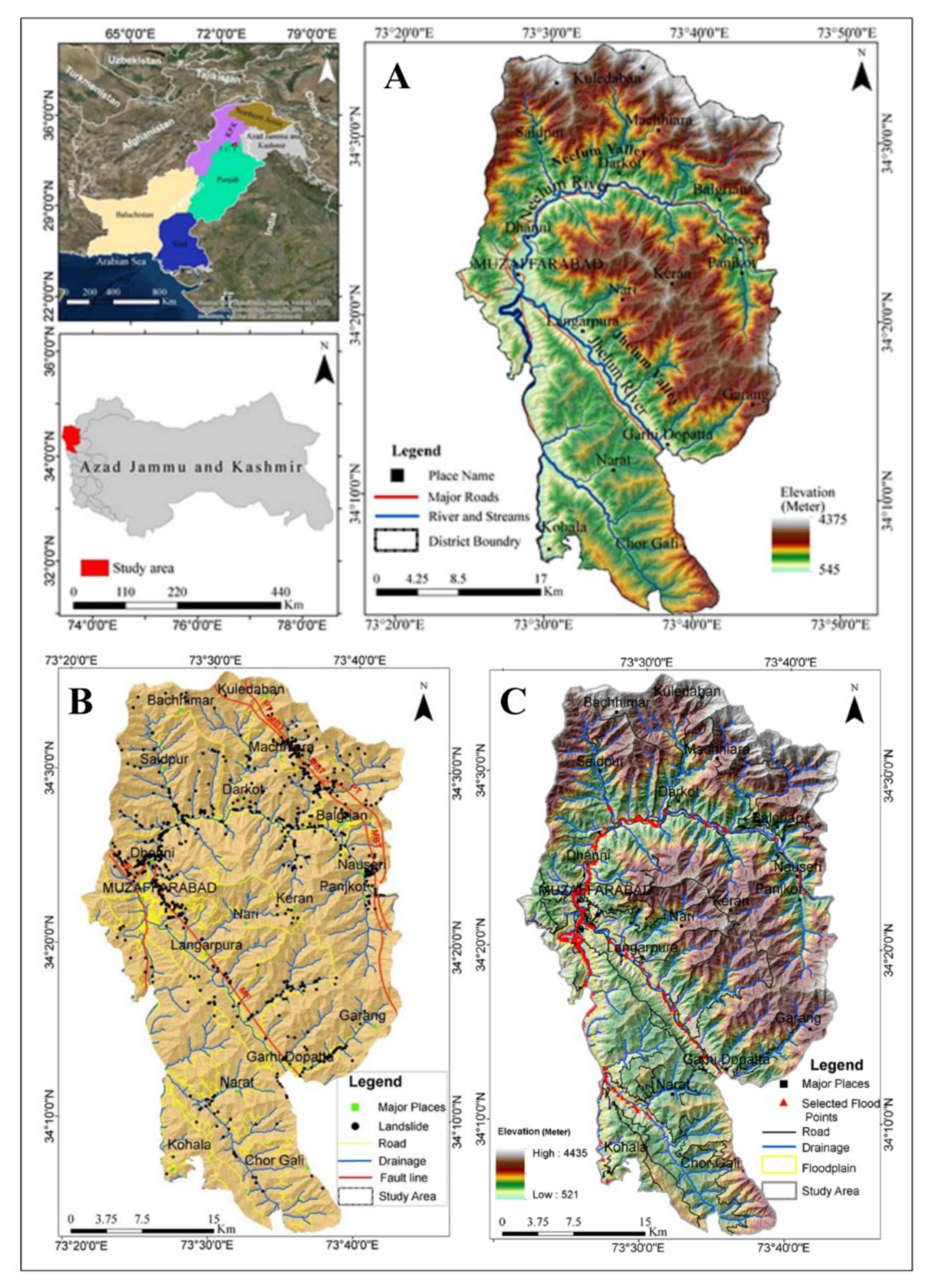
Muzaffarabad District was chosen as our case research area in which to test the multi-hazard susceptibility model. Geographically, the study area is situated between 34°04′00″ N to 34°35′00″ N latitudes and 73°30′45″ E to 73°59′00″ E longitudes, having an area of approximately 1300 square kilometers (Figure 1). Politically, the research area is the capital of the Azad State of Jammu and Kashmir, part of Pakistani Administrated Kashmir (PAK). The Muzaffarabad District contains two tehsils: the first is Muzaffarabad itself, and the second is the Pattika, also known as the Naseerabad. Muzaffarabad City is located on the confluence of the River Neelum and the River Jhelum.
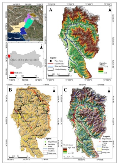
Figure 1.
Study area; (A) location, topography, and drainage; (B) landslide inventory map; and (C) flood inventory map.
The study area’s relief is low in the south (Jhelum Valley), increasing towards the northeast and southeast (Neelum Valley) as high as 4375 m due to the collision zone of the Indian and Eurasian tectonic plates. The research area lies in the humid-to-high subtropical land receiving maximum precipitation (1400 mm) during the summer monsoons (late June to early September). During the summer monsoon, torrential and intense rainfall spells often flood the major rivers and their tributaries. The mean minimum temperature for January and the mean maximum temperature for June are −2.65 °C and 36.75 °C, respectively.
Tectonically, the research area is highly seismically active and part of the northwestern Himalayas. Geologically, the rock formations present in the research area range from Precambrian to Quaternary. Lithologically, the area mainly consists of slate, phyllite, metasediments, metavolcanics, marble, limestone, dolomite, sandstone, shales, unconsolidated silt, sand, and clay deposits.
The research area, including Muzaffarabad City and part of Neelum valley and Jhelum, has a population of 726,000 with an annual growth rate of 2.80% [31]. Being a capital city, all the government, non-government, and nonprofit organization (NGO) offices are located here. All roads that are linked to the major cities are paved and connected with bridges. From an economic point of view, the study area has great importance due to its natural resources and beauty that attracts many tourists locally and internationally.
3. Methodology
Four steps accompanied this research work: (1) geo-hazard inventories and all the causative factors were prepared and their spatial database generated in ArcGIS 10.5 software; (2) the subjective weights (SWs) and objective weights (OWs) of both geo-hazards were calculated using the assembled FR–AHP geospatial techniques, (3) the weights of the individually produced geo-hazard maps were synthesized for the multi-hazard susceptibility assessment; and (4) the accuracy assessment and model validation was assessed to check the performance of the produced multi-hazard susceptibility assessment by using the ROC, SCAI, and frequency ratio methods. A complete methodology flowchart is given in Figure 2.
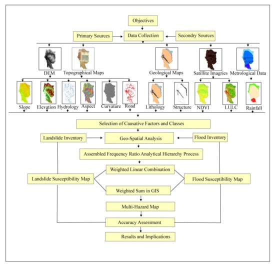
Figure 2.
Methodological flow chart for the multi-hazard susceptibility assessment.
3.1. Data Collection and Selection of the Causative Factors
Data was collected from primary and secondary data sources to accomplish the research objectives. Intensive fieldwork was carried out for the primary data collection. Geological and topographical maps were obtained from the Geological Survey of Pakistan [32]. In addition, satellite images were downloaded from the United States Geological Survey (USGS), Earthexplorer, and the Alaska Satellite Facility (ASF) websites. The complete detail of the data and their sources are shown in Table 1.

Table 1.
Complete details of the data sources and causative factors.
3.2. Field Survey and Preparation of the Inventories
Field visits were carried out to better understand the actual ground conditions and real-time data collection. During the field visits, the spatial distribution of the geo-hazards and their causative factors were well examined. These visits were beneficial for preparing the database inventories for the landslides and floods. The landslide inventory map was prepared from the SPOT-5, QuickBird, Google Earth, and Sentinel 2 satellite images (from 2005 to 2018) using visual interpretation and the supervised image classification tool in the ArcGIS 10.5 software. A total of 670 landslides were identified (Figure 1). The interpretation of all the landslides was identified at a scale of 1:50,000. During the field visits, 68 landslides (app. 5% of the total known/interpreted landslides) were confirmed using the Global Positioning System (GPS) to check the accuracy of the landslide inventory map. A total of 55 landsides out of 68 (80.7% accuracy assessment) was confirmed and accurately located. All the identified landslides were included with equal importance during the analysis, despite their type, size, and shape. The 2010 and 2014 flood events inundation data and flood plain locations were confirmed using high-resolution satellite images and field visits for the flood inventory map. A total of 180 locations out of 208 (86.5% accuracy assessment) were confirmed and accurately located in Figure 1. Later, both fields’ varied landslide and flood locations were used for the model validation and accuracy assessment rather than dividing the data into training and validating data sets, as was suggested by many researchers [26,33,34]. The study area had a very rugged topography and steep slopes. Some remote areas were inaccessible due to a lack of road links. During the field visits, a digital photograph was taken and verified, and the accessible locations were chosen to confirm the accuracy of the inventory maps.
3.3. Geospatial Techniques
Multicriteria decision analysis (MCDA) is a complex phenomenon used to evaluate several causative factors simultaneously. Sometimes, MCDA, also known as Multicriteria Decision Making (MCDM), is a systematic method used to address complex problems by dividing the complex problem into small parts, analyzing them, and integrating them in a meaningful and logical manner. The resultant solution was then obtained in a single composite [35]. MCDA assembled with GIS (GIS–MCDA) effectively provides a wide range of geographically spatial data manipulation costs and time. A GIS–MCDA offers procedures and techniques to evaluate, analyze, design, and prioritize value judgments. Many studies show the importance of GIS–MCDA for hazard assessment [19,36,37,38,39,40]. Many qualitative and quantitative GIS–MCDA techniques and procedures were developed to analyze and manipulate spatial data in recent years. Most widely used geospatial techniques are bivariate and multivariate, such as Frequency Ratio (FR) [12,41,42], AHP [20,22,43,44], logistic regression [9,33,42,45], fuzzy logic [46], the weight of evidence [34,47], and their assembled techniques, such as FR–AHP, FR–WoE, FR, LR–WoE, and LR–AHP [33,47,48]. In this research, the FR–AHP assembled geospatial technique was used to calculate the weights of the selected causative factors and their subclasses.
3.3.1. Analytical Hierarchy Process (AHP)
The AHP was introduced by Saaty [49]. This method is also known as a pairwise comparison method because, in this method, a comparison matrix is used to calculate the weight of the selected factors by calculating the matrix’s eigenvectors [50]. The AHP method is a decision-making process through which a set makes complex decisions regarding the choices or alternatives. Sometimes, these choices/alternatives are qualitative, quantitative, and occasionally conflicting [51,52,53]. In this method, two selected factors are simultaneously evaluated, and preference is given to one factor over another based on experienced judgments. These judgments are measured using a preference scale of 1–9, in which a lower number (1) indicates a lesser preference and a higher number (9) shows more importance of that particular factor over another. The preference score values are given in Table 2, which was used in this research.
Table 2.
Score value for the pairwise comparison after [54].
The AHP method also provides the accuracy assessment and consistency of the weights and rank scores of the priorities (set of alternatives), based on experienced judgments [37,42,55]. The consistency (Consistency Ratio (CR)) can be calculated from the following Equation (1):
where CR is the consistency ratio of a particular AHP matrix, the Consistency Index (CI) can be calculated from Equation (2), and RI is the random index, which depends on the number of factors (n).
where is the consistency vector (average value of each calculated eigenvectors), and “n” represents the number of selected factors. The RI was estimated from 500 different matrices by Saaty [56], and their values are given in Table 3. According to Lootsma [57] and Arabameri, and Rezaei [58], the CR should be within the limits of 10% (CR < 0.01), otherwise the assigned score values should be reconsidered.
Table 3.
Random Index (RI) of the calculated AHP matrices.
3.3.2. Frequency Ratio (FR)
The Frequency Ratio is the most simple and widely bivariate statistical technique, often used in many research types, such as the earth sciences, environmental sciences, hazard assessments, and physical sciences. FR enables the evaluation of the impact of a phenomenon (such as floods and landslides) by the attributes (subclasses) of a causative factor (such as slope, lithology, and curvature). Moreover, the FR is defined by Lee and Pradhan [59] and Lee and Sambath [60], which is the ratio of the probability of a phenomenon occurrence to that of no phenomenon occurrence for any given attribute. According to Yilmaz [61], the FR is the most understandable and straightforward statistical technique. The FR of each causative factor class can be expressed as the ratio of the percent of the class and the percentage of the total hazard (e.g., landslides and floods) in that class [48]. All the causative factors for both selected geo-hazards were classified to calculate the OW. Subsequently, the inventory maps were overlaid for each causative factor, and the FR was calculated within each causative factor class (Figure 3 and Figure 4). A ratio value greater than 1 indicates a substantial correlation with a geo-hazard occurrence and/within a causative factor class, and a ratio value of <1 indicates the weaker relationship [48,62]. For the final rank (weights of a class) calculation, the FR was further integrated with AHP (FR–AHP). The AHP matrix assigned the score values according to their FR value, instead of an expert opinion value judgment.
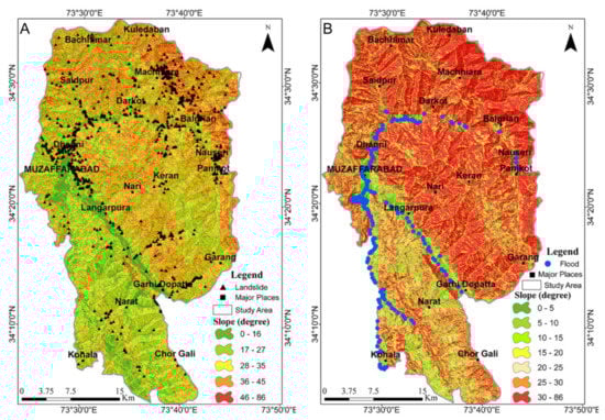
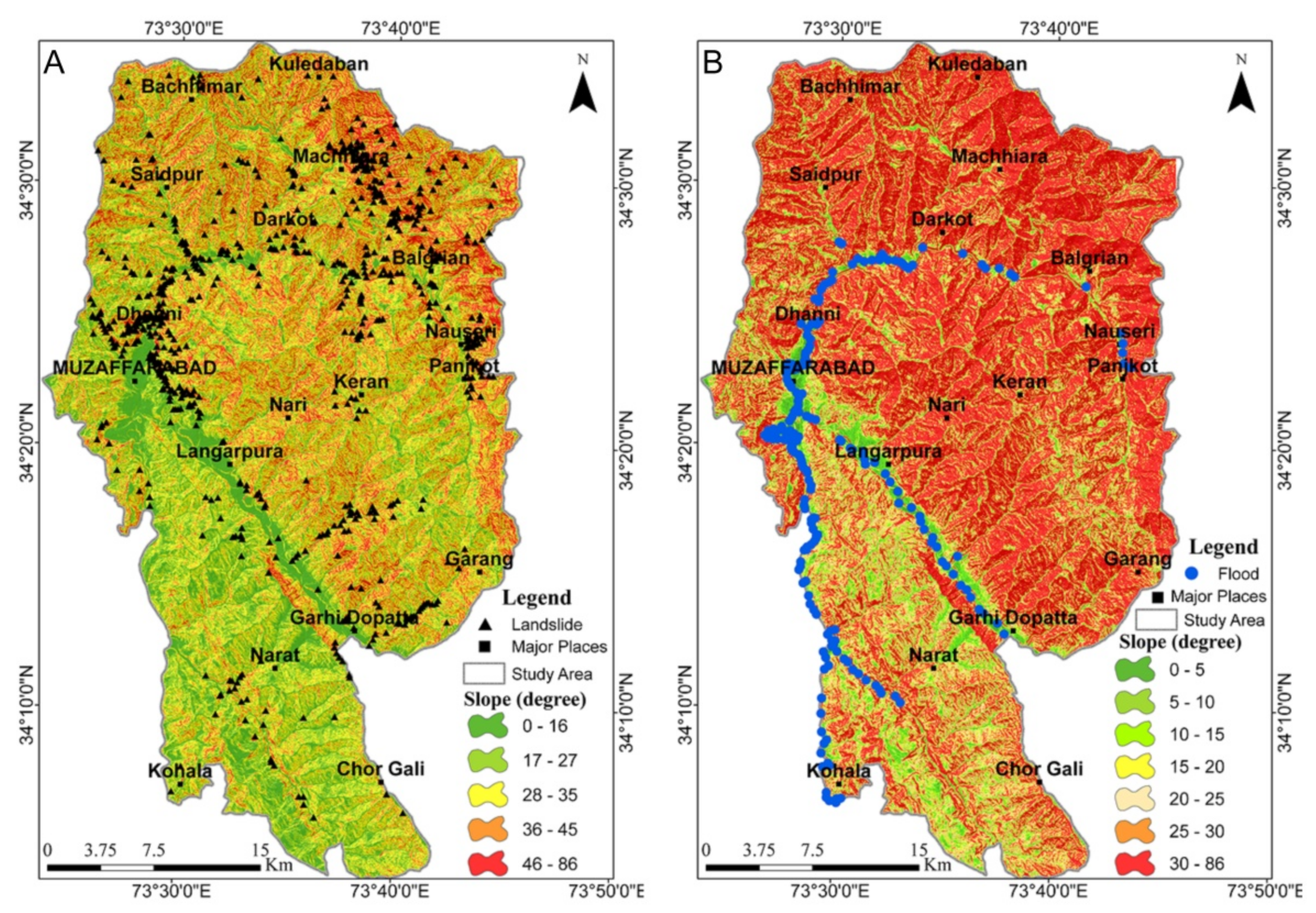
Figure 3.
Slope causative factor maps: (A) landslide and (B) flood.
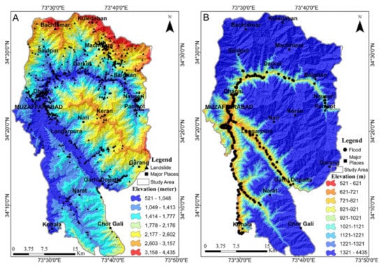
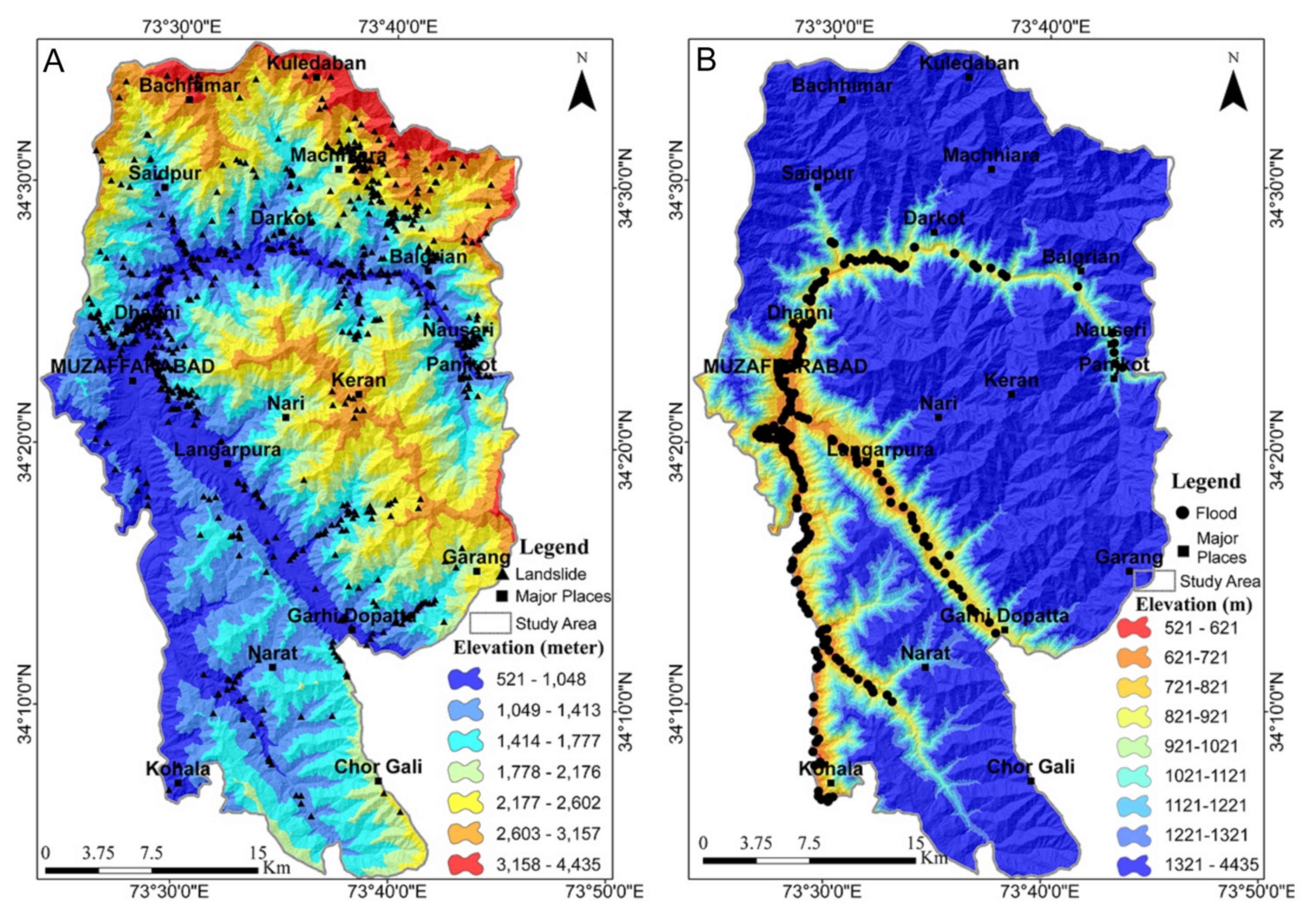
Figure 4.
Elevation causative factor maps: (A) landslide and (B) flood.
3.3.3. Assembled Geospatial Techniques
To avoid the biases and uncertainties of assigning the weights of all causative factors and their classes, the assembled geospatial technique was used in this research, namely as the Frequency Ratio assembled to the Analytical Hierarchy Process (FR–AHP). The aim of selecting the assembled geospatial techniques was to avoid assigning class weights based on so-called experienced judgments or expert opinions. These techniques have proven to be the best fit, together [48,58,63]. The SWs of the geo-hazards, as mentioned above, were evaluated by an intensive literature review, site visits, and experienced judgments. Additionally, a survey was conducted by 10 relevant experts/geoscientists. Their expert opinions and value judgments were then averaged, and an appropriate score value was assigned to each causative factor. The SWs were then determined with the AHP application using the Expert Choice 11 software. First, the FR was calculated for each causative factor class for the determination of the OWs. After that, the final OWs were calculated using the AHP application according to their relevant FR values.
3.4. Multi-Hazard Susceptibility Assessment
On the one hand, geo-hazards, as mentioned above, were produced individually by the application of Weighted Linear Combination (WLC) in ArcGIS 10.5 as follows:
where LSI is the Landslide Susceptibility Index, n is the total number of causative factors, CFi represents the SWs of the causative factors, i and are the OWs that are subjectively determined by the jth class within causative factor i using the AHP [48].
where FSI (Equation (4)) is the flood susceptibility index, n is the total number of causative factors, CFi represents the SWs, and i and are the OWs that are subjectively calculated.
The individual geo-hazard susceptibility maps that we produced in the previous sections were classified into an equal number of classes by using the same classifying scheme, SD. However, the simple summation of individuals producing susceptibility maps is not an appropriate way to create the single multi-hazard map [27]. Since every geo-hazard has different intensity and interaction/consequences with other hazards, sometimes a single hazard triggers multiple hazards [23]. To overcome this problem, [26,27] used the qualitative approach for the relative weight calculation of individual geo-hazards. However, in this paper, we used the same qualitative approach to assess the relevant weight of both geo-hazards based on the historical record and field knowledge.
Furthermore, a questionnaire survey was also conducted by 10 experts. The assigned weights were then averaged and used for the final multi-hazard map. The first preference, with a 70% relative weight, was assigned to LSA because the research area was situated in the northwestern Himalayas, which is highly seismically active. The frequency of landslides can be seen from a single event (the 2005 Kashmir earthquake) that triggered thousands of landslides in the research area [4,10,64,65]. The 30% relative weight was assigned to the FSA. The overall relative weights for the final multi-hazard map were then synthesized by using the following Equation (5):
where MSI is the multi-hazard susceptibility assessment, n represents the number of geo-hazards, Hi is the geo-hazard, and Wi is the relative weight of the geo-hazard i.
3.5. Accuracy Assessment
The accuracy assessment and validation of the models are essential for susceptibility/predicting analysis [22,66]. In the current research work, we used three different techniques, the Receiver Operating Characteristics (ROC) curve, the Seed Cell Area Index (SCAI) method, and the frequency Ratio model, to measure the models’ accuracy and future prediction power.
ROC is a graphical plot that reflects the effectiveness and predictive power of the model in a qualitative hierarchy by calculating the Area Under the Curve (AUC). A higher percentage of the area below the curve indicates a higher accuracy of the model, and the lower area below the curve indicates a lower accuracy of the model to predict the future occurrences of the phenomenon. On the other hand, ROC also quantitatively measures the model accuracy as AUC <0.6 (<60%), 0.6–0.7 (60–70%), 0.7–0.8 (70–80%), and >0.9 (>90%) indicate the modeling accuracy as weak, moderate, good, and very good, respectively [67]. The Success Rate Curve (SRC) and Prediction Rate Curve (PRC) were used for both individual geo-hazards (LSA and FSA) and the multi-hazard map. For calculating the AUC for SRC and PRC, the dependent variables (such as landslides and floods) must be in their proportion of training and validating data sets. The different schemes are available in the literature to divide the data sets (dependent variable) into their training and validated data sets, as 50:50, 60:40, and 70:30, respectively. In this research, to validate the selected model’s actual field data sets were used that were collected during the field visit and the accuracy assessments of the inventories. Many researchers chose the latter classification scheme for its popularity and recommendation [34,47].
The SCAI method represents the area coverage of each hazard susceptibility class in percentage over the seed cells (hazard density in percentage) in each susceptibility class [68,69] as:
SCAI = % area coverage/% seed cell
It is accepted that the SCAI value should be very high for the very low and low susceptibility classes, and the SCAI value should be very low for the high and very high susceptibility classes, accordingly [19,33].
The frequency ratio model is considered as quite popular in the scientific community to evaluate the model accuracy [9,70]. This method is quite similar to the SCAI method but in a reverse manner. The susceptibility maps were first classified by the same classification schemes with an equal number of susceptibility classes using the later models. Subsequently, the inventories maps were superimposed onto each susceptibility class, and the SCAI and Frequency Ratio were calculated.
4. Results
4.1. Preparation of the Geo-Hazard Maps
As mentioned above, the study area was regularly affected by the geo-hazards due to the unfavorable geological conditions, seismicity, rugged topography, and many anthropogenic activities. Based on the extensive literature review, site characteristics and data availability, as well as eleven causative factors, namely the slope, elevation, hydrology, aspect, curvature, road, lithology, structure, NDVI, LULC, and rainfall, were selected for the LSA, out of which eight causative factors, such as the slope, elevation, hydrology, lithology, structure, NDVI, LULC, and rainfall, were chosen for the FSA. The complete detail of each causative factor and individually produced geo-hazard map is presented in the following sections.
4.1.1. Slope
A slope is an important causative factor when considering landslides and floods [30,55]. Usually, steep slope areas are more susceptible to landslides [71] and a low slope gradient, usually flat areas, are more susceptible to flooding [55]. The slope gradient was generated from the DEM image. The slope gradient ranged from 0 to 86 degrees, and was then classified into five and seven numbers of classes for the LSA and FSA. After the classification, the results showed that most of the research area (29.86%) was found in the 28–35° slope class (Figure 3A), and Muzaffarabad City and the other residential areas along the River Jhelum were found in the lowest slope class range (Figure 3B). While comparing these results with the inventory maps, the highest landslide frequency (2.08) was found in the higher slope range (46–86°) and the lowest slope class was found to have the highest flood frequency at 41.88 (Table 4).
Table 4.
AHP matrices and OWs for the slope causative factor classes.
4.1.2. Elevation
The higher altitude areas are important for slope instability analysis, and the low lying areas, such as flat areas, foothills, and valley floors, are more susceptible to flooding when interlinked with discharge channels [14,66,72]. The elevation map was generated by using the DEM image. The altitude difference range, from 521 to 4435 m, was accordingly classified into seven and nine numbers of classes for the LSA and FSA, respectively, as shown in Figure 4A,B. The relationship between the location distribution (inventory) and elevation classes revealed that the lowest elevation class had the highest landslide and flood frequency ratios, as 2.28 and 101.2. The calculated FRs and the OWs of the elevation classes are given in Table 5.
Table 5.
AHP matrices and OWs for the elevation causative factor classes.
4.1.3. Hydrology
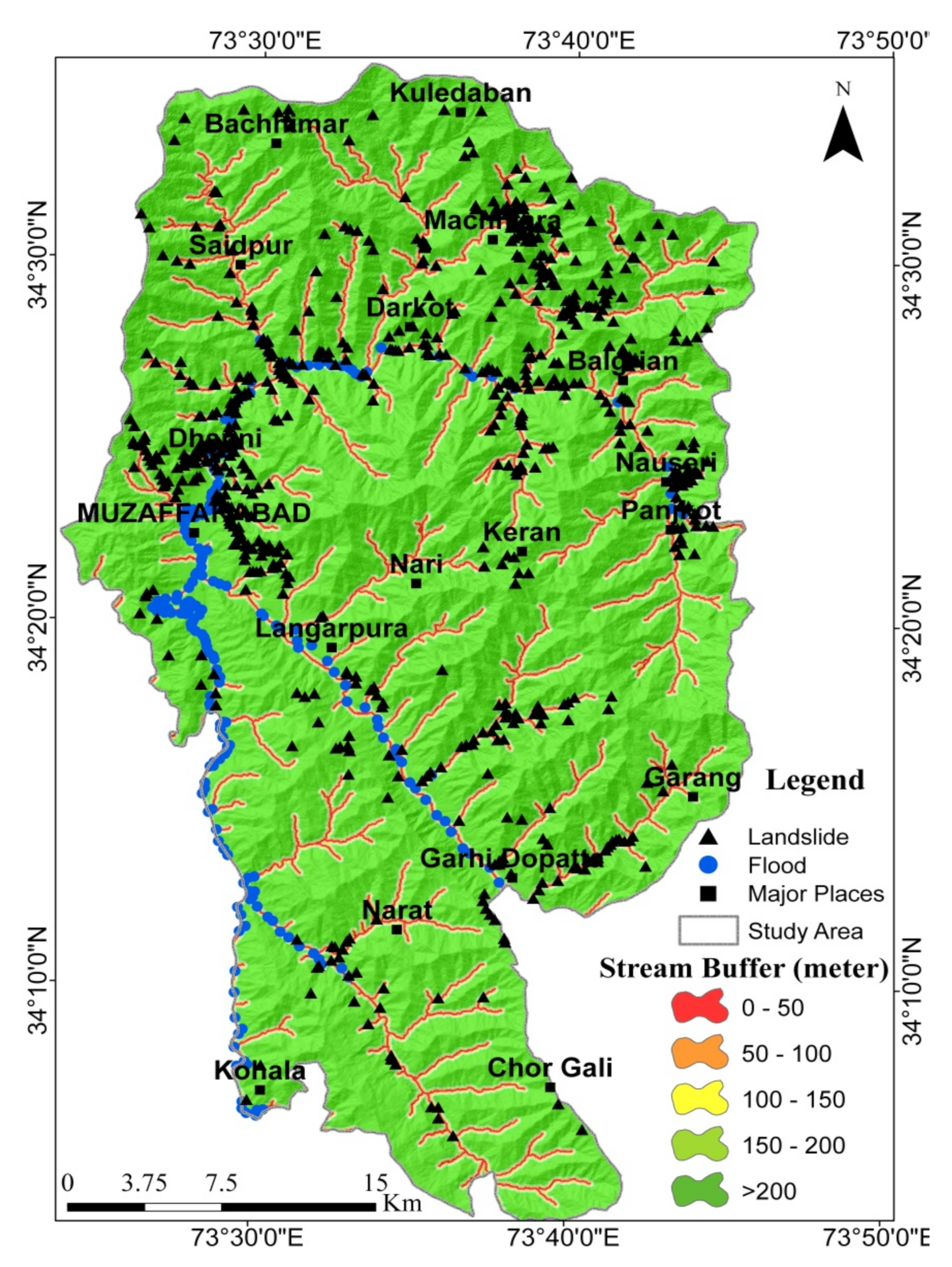
The hydrology of an area directly controls the groundwater [73], flooding [24,40,72], and landslides [12]. The watershed of the research area was delineated from the DEM image by using the Arc hydro tool 10.5 extensions according to the Strahler classification scheme [74]. After delineating the hydrology, the Euclidean distance tool generated the buffer around the streams. The distance buffer was classified into five classes: <50, 50–100, 100–150, 150–200, and >200 m (Figure 5). The calculated buffer distance was considered around all the delineated streams with equal importance because the landslides were found in every stream buffer class. While calculating the FR, all the stream buffer classes were found to have a substantial relationship (FR > 1) for the landslide distribution, except for the stream buffer class range with a distance of >200 m. Additionally, most of the flooded locations were found near the streams and are presented in Table 6.

Figure 5.
Hydrology causative factor map.
Table 6.
AHP matrices and OWs for the hydrology causative factor classes.
4.1.4. Aspect
The slope facing (aspect) is also suggested by [45,75,76], which incorporates sunlight exposure, evapotranspiration, precipitation towards soil erosion, and the vegetation type [77], and was calculated from the DEM image. Most of the research area (16.36%) was found on a southwestern facing slope, and the lowest area (0.05%) was found on a flat surface (Figure 6). The southern facing slopes (SE, S, SW) were found, FR > 1, indicating a positive correlation with the landslides. In contrast, the northern facing slopes (NE, N, NW) showed a weaker relationship with the landslides, occurring as FR < 1 (Table 7). As expected, the flat areas showed no occurrence of landslides (FR = 0).
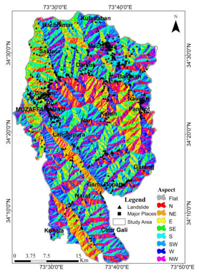
Figure 6.
Aspect causative factor map.
Table 7.
AHP matrices and OWs for the aspect causative factor classes.
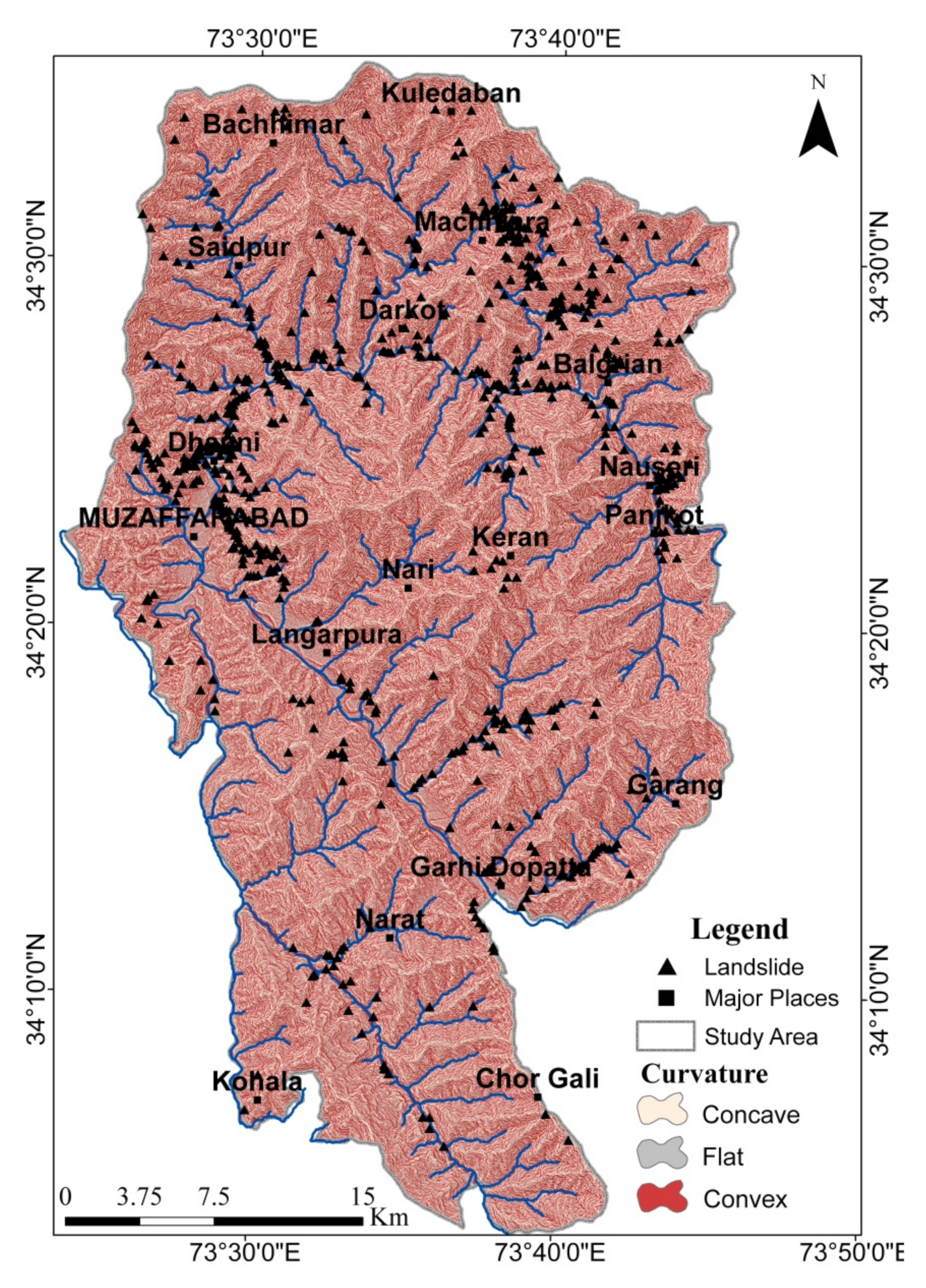
4.1.5. Curvature
The curvature is the slope curve derivative that indicates the slope’s steepness at a certain point by the line tangent, indicating the slope change rate at that particular point. The slope curvature is an essential topographic factor in landslide susceptibility [22,78]. The slope curvature map was generated from the DEM image. The plan curvature type suggested by the above researchers was used. The calculated plane curvature type was classified into three classes: the negative value indicates a concave slope, the values from −0.1 to 1.0 indicate the flat plane, and >0.1 indicates a convex slope, respectively, as shown in Figure 7 [66,76]. After the classifications, the results showed that most of the area lay on both concave and convex classes with an approximate equal-area percentage (47.9 and 48.0), and only 4.1% was found on the flat surface. The relationship between the curvature and landslide distribution indicated that both curvature classes had quite similar landslide distributions, but the concave class shows a slightly higher FR = 1.09. For this reason, the concave class attained a higher OW than the convex class (Table 8).
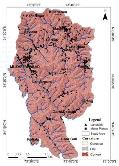
Figure 7.
Curvature causative factor map.
Table 8.
AHP matrices and OWs for the curvature causative factor classes.
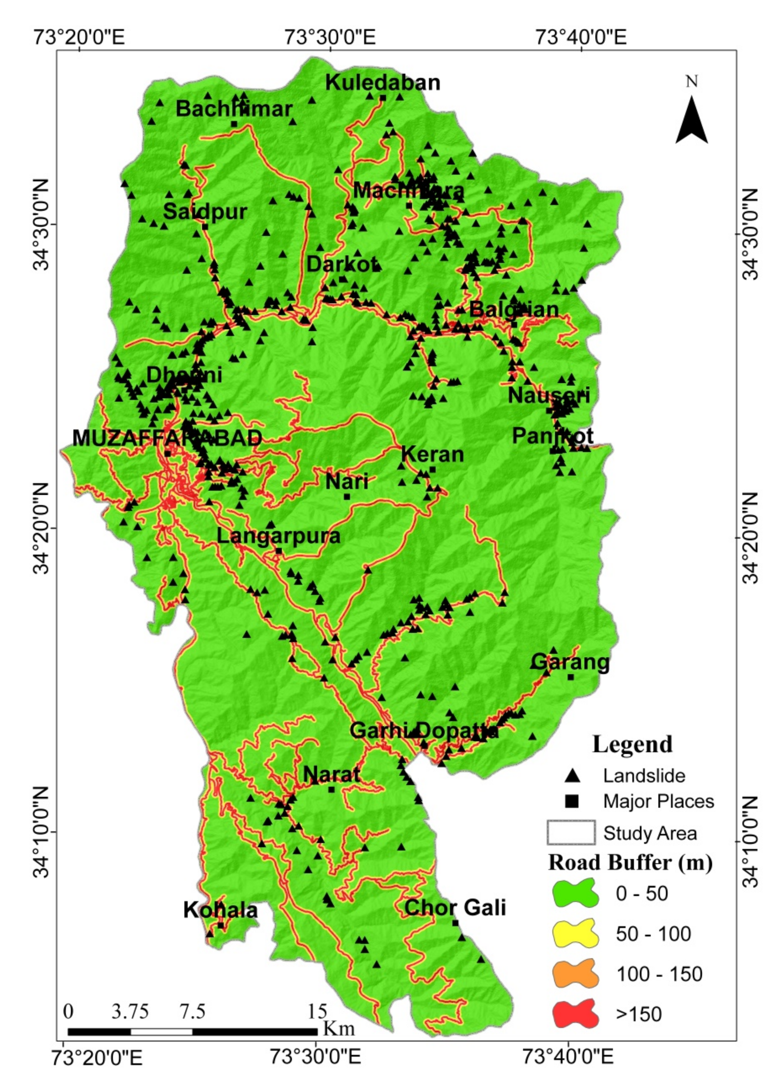
4.1.6. Road
Road construction, especially in the hilly areas, led to mass movement and slope instability due to the undercutting of the steep slope and the removal of material near the foothill [34,59]. The areas under and sides of the road also experienced the heavy load and vibration that caused slope failure. The road networks of the research area were digitized from eight mosaicked topographical maps of 1:50,000 and a high resolution (0.6 × 0.6 m) QuickBird image. The buffer was classified with distances of 0–50, 50–100, 100–150, and >150 m (Figure 8). The highest FR 2.27 was found within a distance of 0–50 m, followed by the 50–100 and 100–150 m as 1.63 and 1.37, respectively (Table 9). The higher FR near the roadsides indicated that the road construction and road cuts positively correlated with the landslides and slope instability in the research area.

Figure 8.
Road causative factor map.
Table 9.
AHP matrices and OWs for the road causative factor classes.
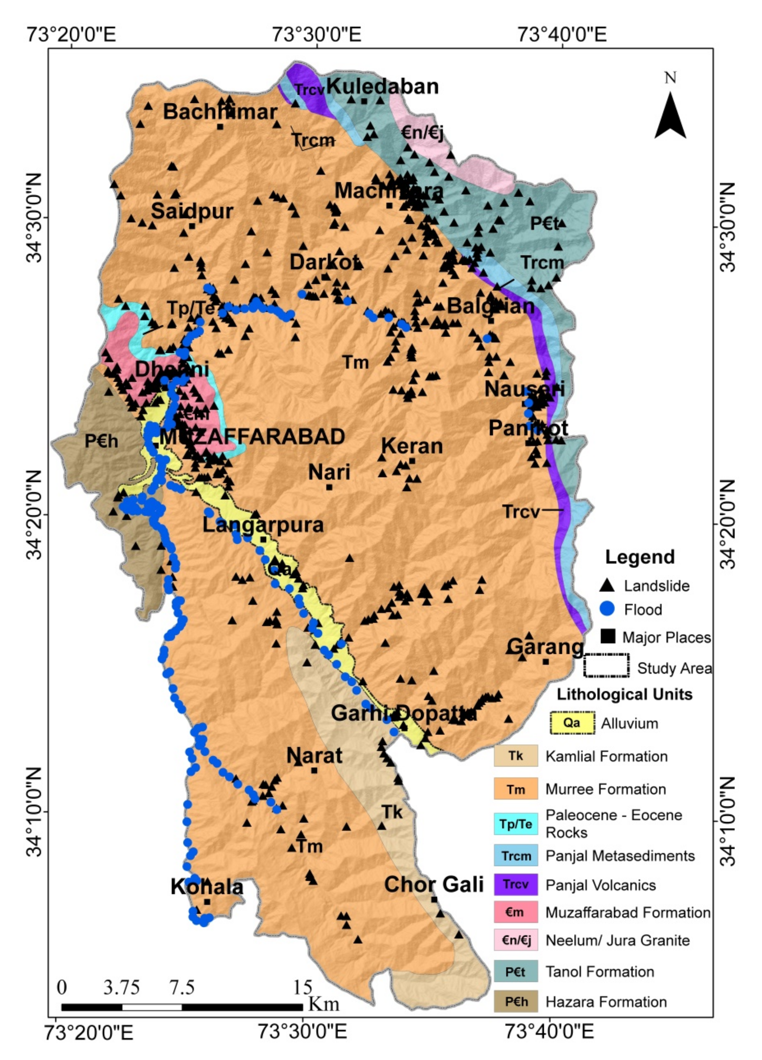
4.1.7. Lithology
An area’s geology (lithological units) is an essential and classic parameter for the geo-hazard susceptibility assessment [5,47,79,80]. The eight geological maps covering the research area at the scale of 1:50,000, were acquired from the Geological Survey of Pakistan (GSP) and published maps [14,81,82,83,84]. The geological map of the research area was constructed and ten different lithological rock formations were identified (Figure 9). The landslide distribution results found that the Muzaffarabad Formation has the highest FR, 5.1, while the Recent Alluvium class showed that the highest flood distribution was 6.85 (Table 10).
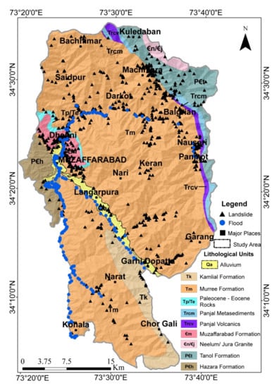
Figure 9.
Lithology causative factor map.
Table 10.
AHP matrices and OWs for the lithology causative factor classes.
4.1.8. Structure
The structural features, such as the lineaments, contact boundaries between different lithological units, and faults lines, produced weaker fracture zones, leading to slope instability [14,66], and control the ground and surface water [85]. The structural map of the research area was digitized from geological [32] and published maps [34]. Four major fault lines were identified as the Panjal Thrust (PT), Main Boundary Thrust (MBT), Muzaffarabad Fault (MF), and Jhelum Fault (JF). A buffer was generated with distances of 0–250, 250–500, 500–750, 750–1000, and >1000 m, presented in Figure 10. The developed buffer also revealed that most of the settlements were near the fault lines, especially Muzaffarabad City, sandwiched between MBT and MF. The landslide distribution results (Table 11) found that the FR possesses a negative correlation with increases in the distance from fault lines. For testing the structure control on flooding, this causative factor was tested for the first time in the research area. However, the smaller lineament features and the contact boundaries between the different lithological units were not included, and only the major faults lines were considered. Table 11 illustrates the OWs and the correlations between the flood locations and the fault buffer classes, with a substantial correlation of FR > 1.
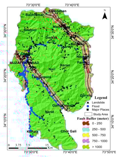
Figure 10.
Structure causative factor map.
Table 11.
AHP matrices and OWs for the road causative factor classes.
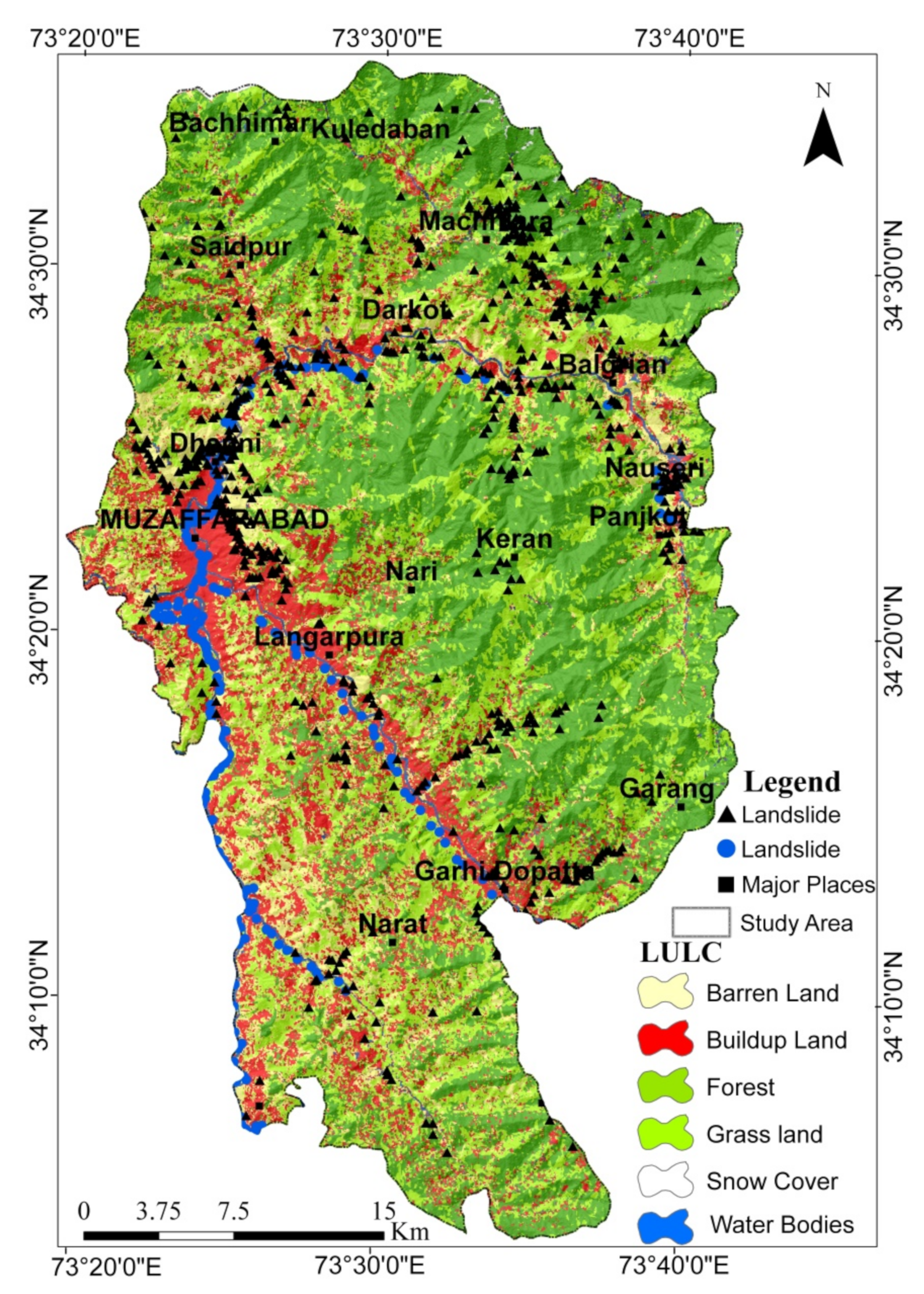
4.1.9. Land Use Land Cover (LULC)
Many anthropogenic factors, such as tunnels, roads, bridges construction, and deforestation, often lead to slope failure [19,22], and these artificial surfaces lead to low or no infiltration and more runoff. Sensitive areas (near the stream channel) are becoming more susceptible to flooding [86,87]. A medium-to-high resolution (10 × 10 m) Sentinel-2 satellite image was used to generate the LULC map of the research area. The “Maximum Likelihood Classification” command was used for supervised image classification [3]. A total of six LULC classes were identified as barren land, built-up land, forest, grassland, snow cover, and water bodies (Figure 11.) The highest OWs were assigned to the barren land (FR = 2.30) and built-up land (FR = 1.27), due to the substantial correlation with landslide occurrences (Table 12). The LULC with the flood locations is given in Figure 11. Three LULC classes, barren land, built-up land, and water bodies, were found to have a strong positive correlation with the flooding, with a value of FR > 1. Other land use classes were found to have a weaker correlation with FR < 1 (Table 12).
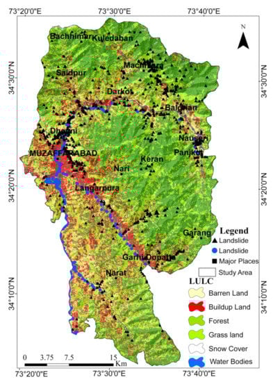
Figure 11.
LULC causative factor map.
Table 12.
AHP matrices and OWs for the LULC causative factor classes.
4.1.10. Normalize Difference Vegetation Index (NDVI)
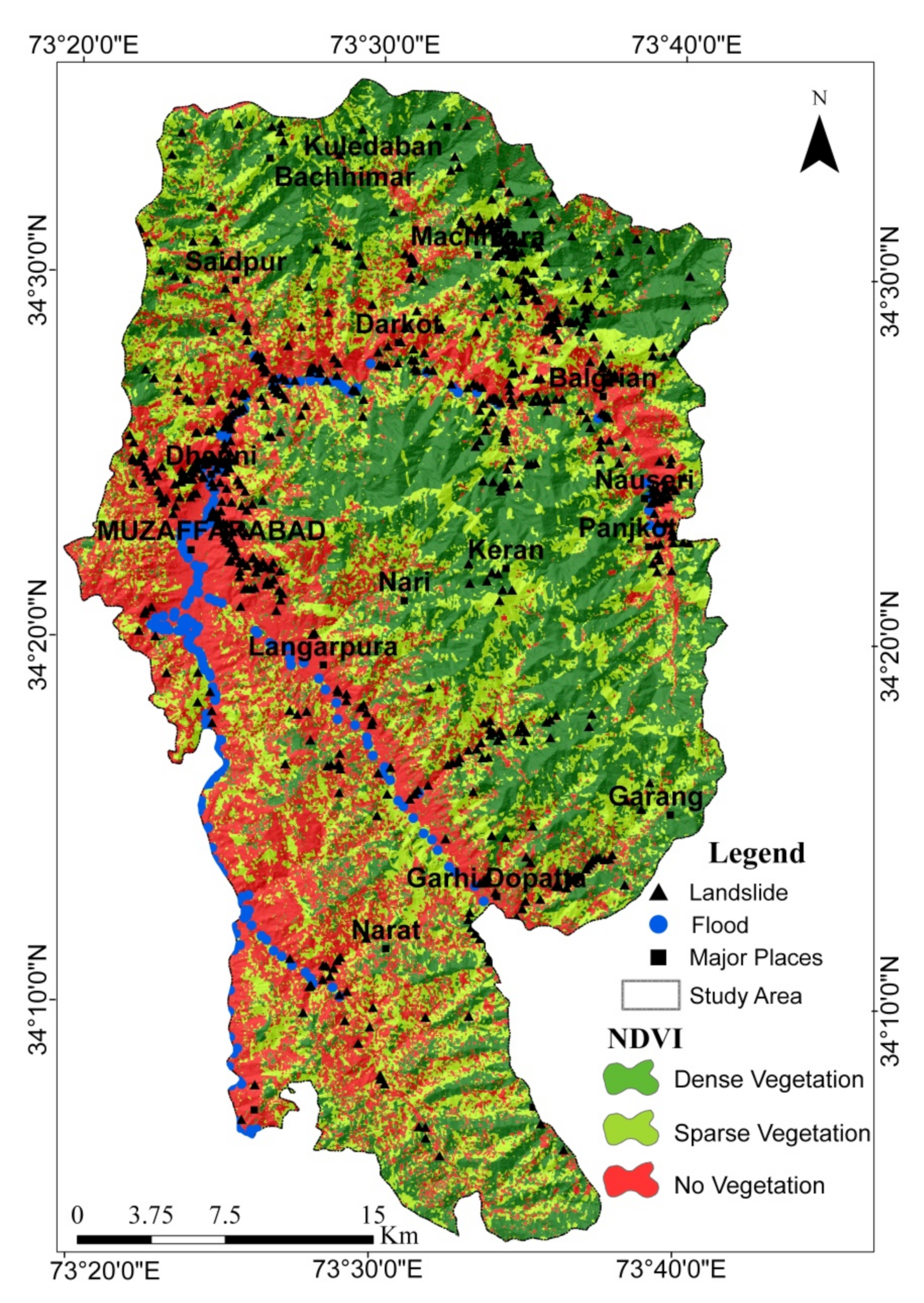
The NDVI represents the vegetation/biomass density of an area. The vegetation cover shows a negative correlation with the slope instability [76] and flooding [88]. The NDVI was calculated from Sentinel-2 images by using the following equation. The derived NDVI ranges from −0.32344 to 0.848607, and was then classified into three vegetation types, densely vegetated areas (forest), sparsely vegetated areas (grassland and rangeland), and no vegetated areas (built-up, barren, and water bodies), which are shown in Figure 12.
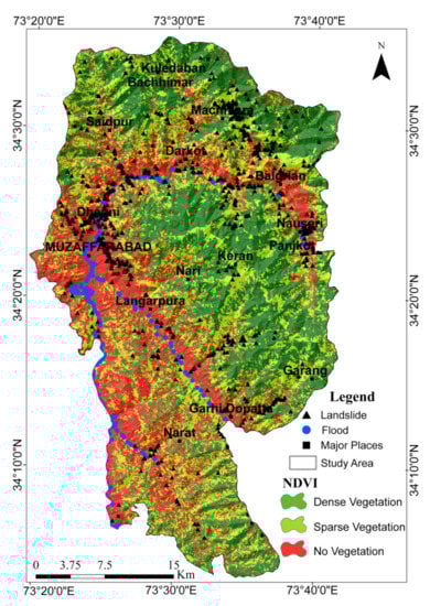
Figure 12.
NDVI causative factor map.
Table 13 represents the FRs and OWs for the distribution of the geo-hazards, and it was found that the no vegetation class had the highest landslide and flood distributions.
Table 13.
AHP matrices and OWs for the NDVI causative factor classes.
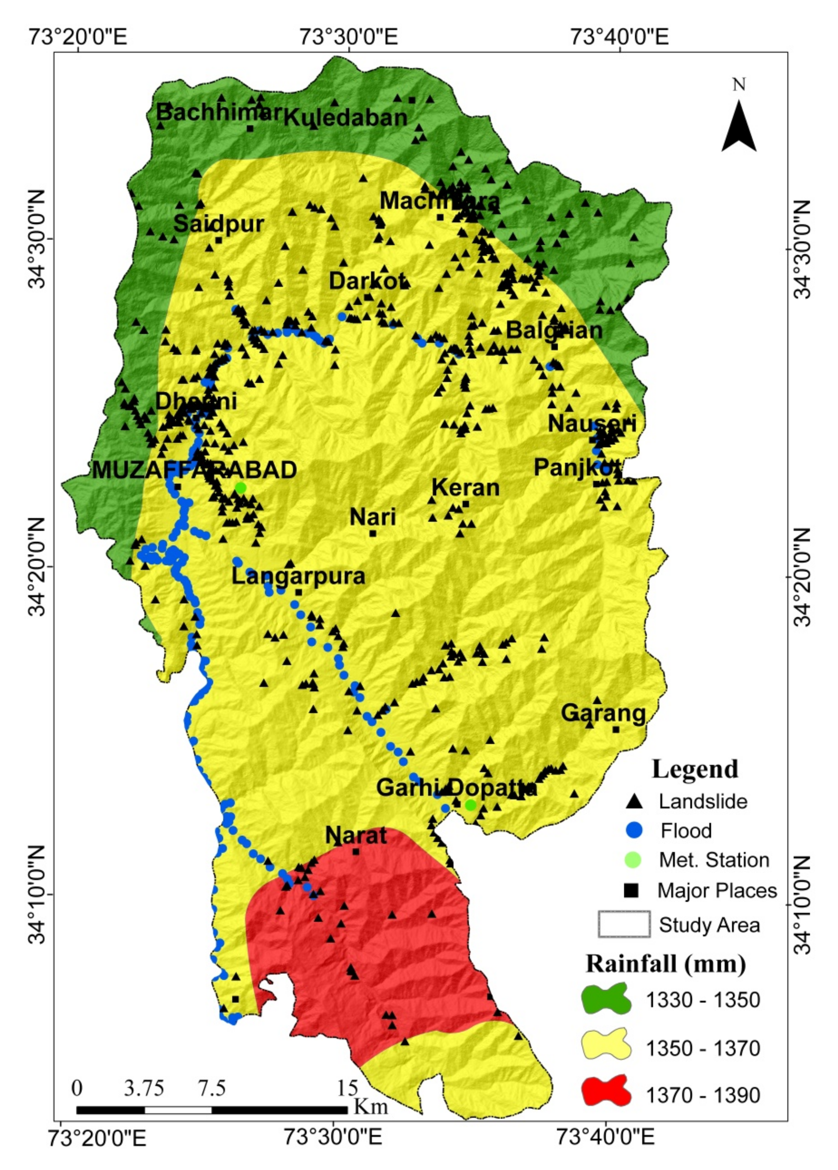
4.1.11. Rainfall
Rainfall is a critical factor responsible for triggering landslides and slope instability [12,20]. The research area lies in the monsoon region and receives most of its rainfall during the summer, which often causes flooding in major and minor streams. Despite its great importance, rainfall is not included in most previous research of the study area. For the construction of the rainfall map, the rainfall data from 20 metrological stations for the last 30 years were used. The rainfall data were averaged, and a database was constructed in ArcGIS. For generating the prediction surface map, a geo–statistical technique Inverse Distance Weighting (IDW) method was used in ArcGIS. The rainfall map was then classified into three classes: 1330–1350, 1350–1370, and 1370–1390 mm (Figure 13). While calculating the FR and OW, it was observed that the medium rainfall class (1350–1370 mm) positively correlated with landslide and flood occurrence (Table 14).

Figure 13.
Rainfall causative factor map.
Table 14.
AHP matrices and OWs for the rainfall causative factor classes.
After determining all the selected causative factor classes, the relevant OWs and SWs were calculated using the FR–AHP method. The complete procedure was discussed earlier in the Methodology Section, and the SWs for the LSA and FSA are given in Table 15 and Table 16, accordingly. The assigned weights influenced the final resultant maps; therefore, great care was taken, and the Consistency Ratio (CR) was firstly prompted, before the generation of the final maps, and both Table 15 and Table 16 show good CRs, as 9% and 7%. Subsequently, all the OWs and SWs were combined, and the Landslide Susceptibility Index (LSI) and Flood Susceptibility Index (FSI) maps were calculated. For the susceptibility classes, the index maps were classified using the standard deviation method into the equal number of classes, very low, low, medium, high, and very high, as suggested by [24,27]. The final LSA and FSA maps are shown in Figure 14A,B.
Table 15.
Detailed AHP matrices for the SWs of the landslide causative factors.
Table 16.
Detailed AHP matrices for SWs of the flood causative factors.
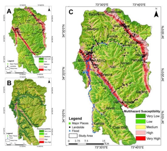
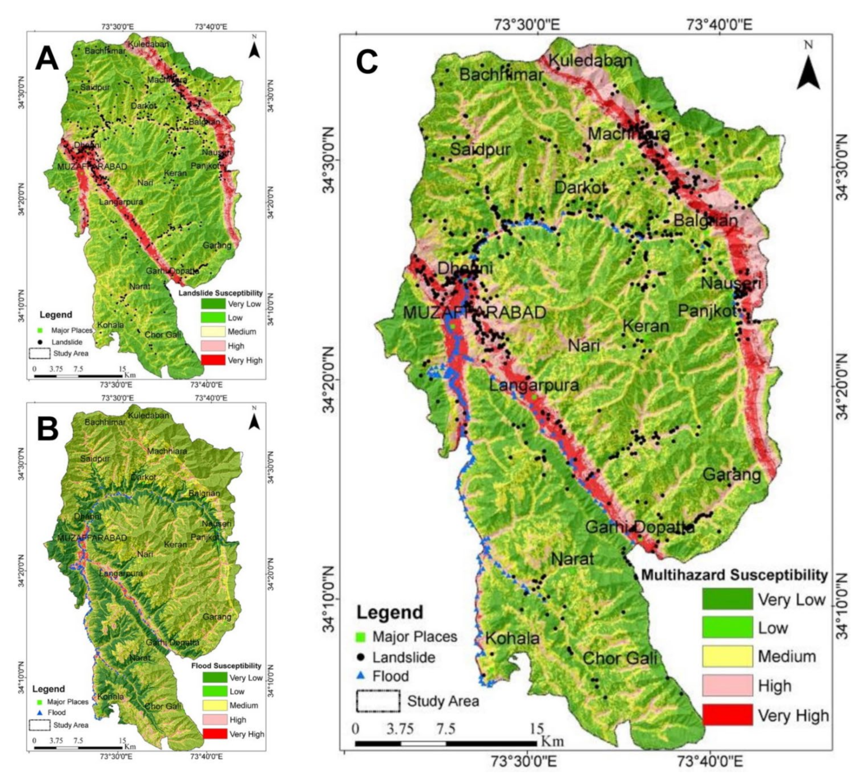
Figure 14.
Susceptibility assessment maps with geo-hazard locations. (A): Landslide susceptibility assessment map, (B): flood susceptibility assessment map, and (C): multi-hazard susceptibility assessment map.
4.2. Multi-Hazard Susceptibility Assessment (MSA)
The individual geo-hazard maps were synthesized using the relative score values of 70% (LSA) and 30 % (FSA) via the weighted sum tool in ArcGIS. The complete procedure is given in the Methodology Section. For the generation of the multi-hazard susceptibility classes, the synthesized index map was classified into five classes, described in the previous section. The multi-hazard map represents both geo-hazards. To verify the impact, both historical events in the form of inventories were overlaid with a multi-hazard map, and the highest densities of both geo-hazards were found in the very high and high susceptibility zones (Figure 14C).
5. Discussion
5.1. Landslide Susceptibility Assessment (LSA) Map
The LSA map was derived by calculating the assembled FR–AHP and GIS methods. Accordingly, the derived map was classified into five classes: very low, low, medium, high, and very high susceptibility zones (Figure 14A). The landslide inventory map was then superimposed over the LSA map to check the landslide impact on the research area. The calculated result within each landslide susceptibility zone is given in Table 17. More than 50% of the land area was found within the very low and low susceptibility zones, and the lowest land area (app 16%) was found within the high and very high susceptibility zones. In contrast, the lowest landslide density was found in the first two zones and the latter zones showed the highest landslide occurrence. The results also indicate that the northwestern and southeastern areas, such as Muzaffarabad City, including the vicinity areas of Dhani, Nausari, and Langarpura, are the most landslide-affected areas due to the active seismicity, unfavorable lithological conditions, and many anthropogenic activities, and these results can be seen from the SWs in Table 15, and correlated with the previous research [5,11,64,84,89].
Table 17.
Individual and multi-hazard susceptibility classes with the area coverage, hazard distribution, SCAI, and frequency values.
5.2. Flood Susceptibility Assessment (FSA) Map
According to Figure 14B, the high and very high flood susceptibility zones are near the major streams. Muzaffarabad City was found within a very high susceptibility zone, in which major streams converge. When comparing this with the historical events (flood inventory), it is also evident that 83% of the flood locations were situated within very high and high flood susceptibility zones. The areal extent and spatial distribution of flood events within each flood susceptibility zone are given in Table 17. The SW also indicates that the major streams and tributaries are responsible for triggering and enhancing the flood susceptibility, followed by the elevation, slope, and lithology (Table 16). The distance from fault lines, which we considered the first time in the research area, showed less importance for the SW calculation of 0.083 (8.3%). Still, objectively, the area near the fault zones shows a substantial correlation with the flood events (Table 11 and Figure 14B).
5.3. Multi-Hazard Susceptibility Assessment (MSA) Map
The result of the MSA map is shown in Figure 14C, which directed the distribution of both geo-hazards in the research area. The majority of these geo-hazards were found in the high and very high susceptibility zones, indicating that the research area was severely affected in the past. The percentage of the area coverage of the multi-hazard susceptibility zones and geo-hazard densities are given in Table 17. The calculated results from the relative weights that we assigned during the production of the MSA map also proved the best fit for the MSA model, for predicting both geo-hazards in the research area. Regarding the high and very high susceptibility zones, most of the settlements already fall into these zones, indicating the great potential for harm during the next geo-hazard event. In addition to this, the model also predicted the very low and low susceptibility zones in the southern, western, and further northeastern parts suitable for future planning. However, these parts lie in remote areas.
5.4. Accuracy Assessment and Validation of the Selected Model
The accuracy assessment and validation of the models are important for susceptibility analysis [22,66]. We used three different techniques, Receiver Operating Characteristics (ROC) curve, Seed Cell Area Index (SCAI), and Frequency Ratio model, to measure the models’ accuracy and future prediction power.
To observe the smooth results of the generated multi-hazard maps and their ability to predict geo-hazards, both the Success Rate Curve (SRC) and Prediction Rate Curve (PRC) were used.
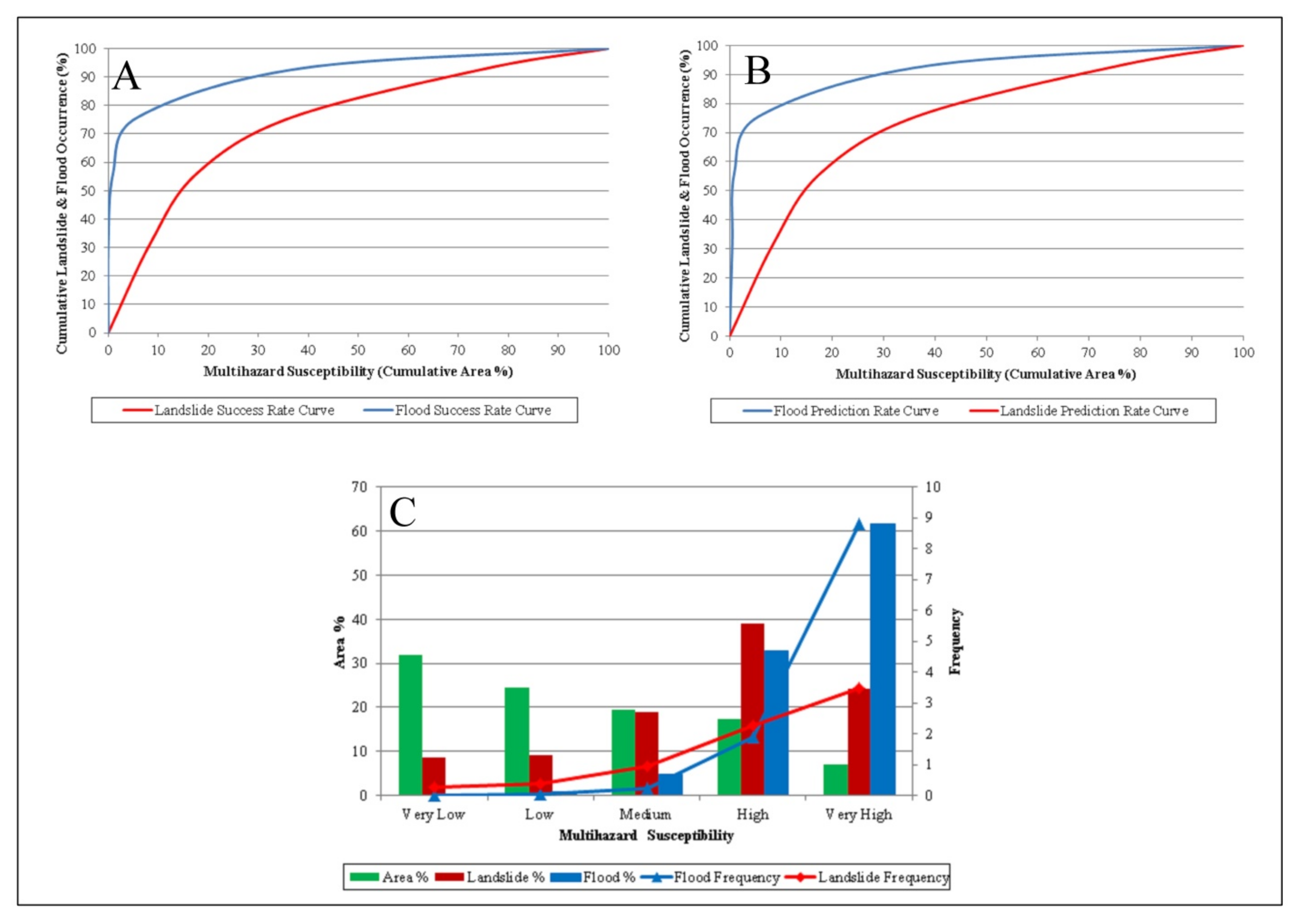
The AUC was calculated by plotting the cumulative susceptibility area percentage on the x-axis and the cumulative landslide and flood occurrence percentages on the y-axis on a scatterplot. The success rates (SRCs) for the LSM and FSM were calculated as 0.743 (74.3%) and 0.958 (95.8%), respectively. For the MSA, the SRC was calculated as 0.743 (74.3%) and 0.906 (90.6%) for both geo-hazards, as shown in Figure 15A and Table 17. Only the SRC cannot represent the efficiency of predicting the power of the models. To measure the real predicting power of the models, the same procedure was repeated for the PRC; however, instead of using training data-set, the validating data sets of known landslides and flood locations were used, which were collected during the field visits for the construction inventory maps. After calculating the AUC, the findings showed results that were relatively similar to those that we calculated for the SRC. This indicated the best fit of the models to predict the occurrence of future geo-hazards (Table 17). The calculated PRC and their details are given in Figure 15B.
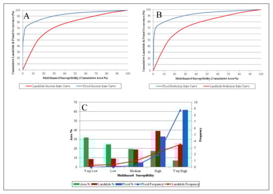
Figure 15.
Validation of the multi-hazard susceptibility models. (A): Success rate curve, (B): prediction rate curve, and (C): frequency ratio.
The second approach for testing the accuracy of the used models and the efficiency of the predicting power was carried out using the SCAI method, suggested by [68,69].
This method represents the area coverage of each susceptibility class in percentage, over the seed cells (hazard density in percentage) in each susceptibility class. Using the SCAI, it is accepted that the SCAI value should be very high for very low and low susceptibility classes, and should be very low for high and very high susceptibility classes, respectively [19,33]. The calculated SCAI shows all the models’ goodness of fit because all the classified maps show the very high SCAI values for the very low and low susceptibility classes and vice versa (Table 17).
Reclassified susceptibility maps were also validated using the frequency ratio suggested by [9,70]. This method is quite similar to the SCAI method, but in a reverse manner. The susceptibility maps were first classified by the same classification schemes with an equal number of susceptibility classes using the Frequency Ratio model. Following this, the inventory maps were superimposed onto each susceptibility class, and the frequency ratio was calculated.
Theoretically, it is accepted that the frequency of the phenomenon will gradually increase from very low to very high susceptibility classes. The calculated results are given in Table 17, indicating that the Frequency Ratios of LSA, FSA, and MSA gradually increase from very low to high susceptibility classes (Figure 15C).
6. Conclusions
Landslides are more common and disastrous in a high terrain that has a fragile slope. The rugged topography, active seismicity, unfavorable geological conditions, heavy monsoon rainfall, and rapid urban growth increase the susceptibility of Muzaffarabad to landslides. After the interpretation of the results, it can be concluded that the following geo-environmental conditions play a vital role in triggering landslides: the slope ranges from 46 to 86 degrees; elevation variations between 521 to 1048 m; stream buffers between 50–100 m; rainfall ranges between 1350–1370 mm in a southern facing slope; positive plane curvature values; unconsolidated and highly fractured rock units; fault distances of 0–250 m; and variations in the LULC. Multicriteria analysis integrated with geospatial techniques was used for the LSA. Additionally, an effort was made to develop a suitable model for the LSA and geo-visualizations by utilizing the historical records. The validations of the model show quite satisfactory goodness of fit and future predicting power as 74.3% and 73.8%, respectively. The selected model produced the satisfactory goodness of fit (74.3% and 90.6%) and predictive power (73.1% and 90.1%) to identify both selected geo-hazards. It can also be concluded that the LSA model is cost-effective and can be used in other geographical locations with the same geo-environmental conditions.
Flooding is a major threat to Pakistan. During the summer monsoon, major and minor streams flooded and often inundated nearby agricultural and populated areas. The Muzaffarabad District was selected to test the susceptibility model due to its ever-growing population and many economic activities near the stream channels without proper planning and site investigations. After the interpretation of all the results, it can be concluded that flood distribution is primarily governed by geo-environmental conditions, such as the slope degrees <5°; elevation <621 m; distance from both minor and major streams (stream buffer) 0–50 m; unconsolidated silt, clay, and gravel deposits; distance from major faults (fault buffer) 500–700 m; no vegetation of NDVI; water bodies and settlements of the LULC; and rainfall class between 1350–1370. In this research, multicriteria geospatial techniques were used for FSA, based on the flood inventory map after the 2010 and 2014 flood events. The implemented susceptibility model showed a goodness of fit of 90.6% and a predicting power of 90.1%, by using the ROC area under-curve. We can also concluded that the FSA model is a cost- and time-effective model that can be used in other geographical locations with the same geo-environmental conditions.
The multi-hazard susceptibility model further concluded that there is a positive correlation between the floods and landslides that affect the research area. The multi-hazard analysis used in the current study yielded reliable results in the delineating regions appropriate for urban development, based on the location of previous landslides and flood events.
The current research provides the initial baseline for multi-hazard susceptibility assessment in the northwest Himalayas. The current study’s implications will help to understand the most susceptible areas to minimize the risks for all stakeholders, even though the current study consisted of two geo-hazards due to the tight time frame and resource allocation. Nevertheless, the proposed model shows the goodness of fit; therefore, it is strongly recommended that more geo-hazards be added for future detailed susceptibility assessments.
Author Contributions
Conceptualization, A.R. and J.S.; methodology, A.R.; software, M.I.A.; validation, A.R., F.H., and S.M.; formal analysis, A.R. and M.B.; investigation, M.S.; resources, M.S.M. and J.S.; data curation, A.R.; writing—original draft preparation, A.R.; writing—review and editing, A.R., J.S., and M.I.A.; visualization, M.S.; supervision, J.S.; project administration, J.S.; funding acquisition, J.S. All authors have read and agreed to the published version of the manuscript.
Funding
This study was supported by the Program for Key Science and Technology Innovation Team in Shaanxi Province (Grant No. 2014KCT-27).
Acknowledgments
We thank all of our lab mates and team members for their valuable suggestions and cooperation.
Conflicts of Interest
The authors declare no conflict of interest.
References
- Uitto, J.I. The geography of disaster vulnerability in megacities: A theoretical framework. Appl. Geogr. 1998, 18, 7–16. [Google Scholar] [CrossRef]
- Cannon, T. Vulnerability analysis and the explanation of ‘natural’disasters. Disasters Dev. Environ. 1994, 1, 13–30. [Google Scholar]
- Rehman, A.; Song, J.; Haq, F.; Ahamad, M.I.; Sajid, M.; Zahid, Z. Geo-physical hazards microzonation and suitable site selection through multicriteria analysis using geographical information system. Appl. Geogr. 2021, 135, 102550. [Google Scholar] [CrossRef]
- Sudmeier-Rieux, K.; Jaboyedoff, M.; Breguet, A.; Dubois, J. The 2005 Pakistan Earthquake Revisited: Methods for Integrated Landslide Assessment. Mt. Res. Dev. 2011, 31, 112–121. [Google Scholar] [CrossRef]
- Basharat, M.; Rohn, J.; Ehret, D.; Baig, M.S. Lithological and structural control of Hattian Bala rock avalanche triggered by the Kashmir earthquake 2005, sub-Himalayas, northern Pakistan. J. Earth Sci. 2012, 23, 213–224. [Google Scholar] [CrossRef]
- The International Federation of Red Cross and Red Crescent Societies. World Disasters Report. 2003, pp. 6–243. Available online: http://www.eurospanonline.com (accessed on 20 November 2021).
- Rafiq, L.; Blaschke, T. Disaster risk and vulnerability in Pakistan at a district level. Geomat. Nat. Hazards Risk 2012, 3, 324–341. [Google Scholar] [CrossRef]
- Asian Development Bank and World Bank. Preliminary Damage and Need Assessment (Pakistan Earthquake 2005). 2005, pp. 1–124. Available online: http://hdl.handle.net/10986/29570 (accessed on 23 July 2019).
- Peduzzi, P. Landslides and vegetation cover in the 2005 North Pakistan earthquake: A GIS and statistical quantitative approach. Nat. Hazards Earth Syst. Sci. 2010, 10, 623–640. [Google Scholar] [CrossRef]
- Basharat, M. The Distribution, Characteristics and Behaviour of Mass Movements Triggered by the Kashmir Earthquake 2005, NW Himalaya, Pakistan. Ph.D. Thesis, University of Erlangen-Nuremberg, Erlangen, Germany, 2012. [Google Scholar]
- Farooq, M.; Qasim, M.; Mateen, A.; Tariq, M.; Nisar, U.B.; Bukhari, A. GIS-based landslide susceptibility zonation mapping along the Muzaffarabad-Chakoti road in western Himalayan region of Pakistan. J. Himal. Earth Sci. 2012, 45, 41. [Google Scholar]
- Rahman, G.; Rahman, A.U.; Collins, A. Geospatial analysis of landslide susceptibility and zonation in shahpur valley, eastern hindu kush using frequency ratio model. Proc. Pak. Acad. Sci. 2017, 54, 149–163. [Google Scholar]
- Petley, D.; Dunning, S.; Rosser, N.; Kausar, A.B. Incipient landslides in the Jhelum Valley, Pakistan following the 8th October 2005 earthquake. In Disaster Mitigation of Debris Flows, Slope Failures and Landslides; Universal Academy Press, Inc.: Tokyo, Japan, 2006; pp. 47–55. [Google Scholar] [CrossRef]
- Basharat, M.; Rohn, J.; Baig, M.S.; Khan, M.R. Spatial distribution analysis of mass movements triggered by the 2005 Kashmir earthquake in the Northeast Himalayas of Pakistan. Geomorphology 2014, 206, 203–214. [Google Scholar] [CrossRef]
- Cheong, J.; Yuan, H. Trade to aid: EU’s temporary tariff waivers for flood-hit Pakistan. J. Dev. Econ. 2017, 125, 70–88. [Google Scholar] [CrossRef] [Green Version]
- Rana, I.A.; Routray, J.K. Integrated methodology for flood risk assessment and application in urban communities of Pakistan. Nat. Hazards 2018, 91, 239–266. [Google Scholar] [CrossRef]
- World Bank. Pakistan Floods 2010: Preliminary Damage and Needs Assessment Project; World Bank: Washington, DC, USA, 2010. (In English) [Google Scholar]
- UN. Johannsburg Plan of Implementation of the World Summit on Sustainable Development; Technical Report; United Nations: New York, NY, USA, 2002. [Google Scholar]
- Akgun, A.; Türk, N. Landslide susceptibility mapping for Ayvalik (Western Turkey) and its vicinity by multicriteria decision analysis. Environ. Earth Sci. 2009, 61, 595–611. [Google Scholar] [CrossRef]
- Kamp, U.; Owen, L.A.; Growley, B.J.; Khattak, G.A. Back analysis of landslide susceptibility zonation mapping for the 2005 Kashmir earthquake: An assessment of the reliability of susceptibility zoning maps. Nat. Hazards 2009, 54, 1–25. [Google Scholar] [CrossRef]
- Hashmi, H.N.; Siddiqui, Q.T.M.; Ghumman, A.R.; Kamal, M.A. A critical analysis of 2010 floods in Pakistan. Afr. J. Agric. Res. 2012, 7, 1054–1067. [Google Scholar]
- Basharat, M.; Shah, H.R.; Hameed, N. Landslide susceptibility mapping using GIS and weighted overlay method: A case study from NW Himalayas, Pakistan. Arab. J. Geosci. 2016, 9, 292. [Google Scholar] [CrossRef]
- Gill, J.C.; Malamud, B.D. Hazard interactions and interaction networks (cascades) within multi-hazard methodologies. Earth Syst. Dyn. 2016, 7, 659–679. [Google Scholar] [CrossRef] [Green Version]
- Bathrellos, G.D.; Skilodimou, H.D.; Chousianitis, K.; Youssef, A.M.; Pradhan, B. Suitability estimation for urban development using multi-hazard assessment map. Sci. Total Environ. 2017, 575, 119–134. [Google Scholar] [CrossRef]
- Kaur, H.; Gupta, S.; Parkash, S.; Thapa, R. Application of geospatial technologies for multi-hazard mapping and characterization of associated risk at local scale. Ann. GIS 2018, 24, 33–46. [Google Scholar] [CrossRef] [Green Version]
- Pourghasemi, H.R.; Gayen, A.; Panahi, M.; Rezaie, F.; Blaschke, T. Multi-hazard probability assessment and mapping in Iran. Sci. Total Environ. 2019, 692, 556–571. [Google Scholar] [CrossRef]
- Skilodimou, H.D.; Bathrellos, G.D.; Chousianitis, K.; Youssef, A.M.; Pradhan, B. Multi-hazard assessment modeling via multi-criteria analysis and GIS: A case study. Environ. Earth Sci. 2019, 78, 47. [Google Scholar] [CrossRef]
- El Morjani, Z.E.A.; Ebener, S.; Boos, J.; Ghaffar, E.A.; Musani, A. Modelling the spatial distribution of five natural hazards in the context of the WHO/EMRO Atlas of Disaster Risk as a step towards the reduction of the health impact related to disasters. Int. J. Health Geogr. 2007, 6, 8. [Google Scholar] [CrossRef] [PubMed] [Green Version]
- Van Westen, C.J. Remote sensing and GIS for natural hazards assessment and disaster risk management. Treatise Geomorphol. 2013, 3, 259–298. [Google Scholar]
- Ma, C.; Wu, X.; Li, B.; Hu, X. The susceptibility assessment of multi-hazard in the Pearl River Delta Economic Zone, China. Nat. Hazards Earth Syst. Sci. Discuss. 2018, 1–30. [Google Scholar] [CrossRef]
- AJK P&D. Azad Kashmir at a Glance; Statistics Section, Planning & Development Department, Azad Govt. of the State of Jammu and Kashmir: Muzaffarabad, Pakistan, 2015. [Google Scholar]
- GSP. Geological Survey of Pakistan. 2004. Available online: https://gsp.gov.pk/ (accessed on 12 September 2019).
- Khosravi, K.; Nohani, E.; Maroufinia, E.; Pourghasemi, H.R. A GIS-based flood susceptibility assessment and its mapping in Iran: A comparison between frequency ratio and weights-of-evidence bivariate statistical models with multi-criteria decision-making technique. Nat. Hazards 2016, 83, 947–987. [Google Scholar] [CrossRef]
- Riaz, M.T.; Basharat, M.; Hameed, N.; Shafique, M.; Luo, J. A Data-Driven Approach to Landslide-Susceptibility Mapping in Mountainous Terrain: Case Study from the Northwest Himalayas, Pakistan. Nat. Hazards Rev. 2018, 19, 1–20. [Google Scholar] [CrossRef]
- Malczewski, J. GIS and Multicriteria Decision Analysis; John Wiley & Sons: New York, NY, USA, 1999; p. 392. [Google Scholar]
- Malczewski, J. GIS-based land-use suitability analysis: A critical overview. Prog. Plan. 2004, 62, 3–65. [Google Scholar] [CrossRef]
- Malczewski, J. GIS-based multicriteria decision analysis: A survey of the literature. Int. J. Geogr. Inf. Sci. 2006, 20, 703–726. [Google Scholar] [CrossRef]
- Chen, Y.; Yu, J.; Khan, S. Spatial sensitivity analysis of multi-criteria weights in GIS-based land suitability evaluation. Environ. Model. Softw. 2010, 25, 1582–1591. [Google Scholar] [CrossRef]
- Greene, R.; Devillers, R.; Luther, J.E.; Eddy, B.G. GIS-Based Multiple-Criteria Decision Analysis. Geogr. Compass 2011, 5, 412–432. [Google Scholar] [CrossRef]
- Rahmati, O.; Zeinivand, H.; Besharat, M. Flood hazard zoning in Yasooj region, Iran, using GIS and multi-criteria decision analysis. Geomat. Nat. Hazards Risk 2015, 7, 1000–1017. [Google Scholar] [CrossRef] [Green Version]
- Yilmaz, I. Landslide susceptibility mapping using frequency ratio, logistic regression, artificial neural networks and their comparison: A case study from Kat landslides (Tokat—Turkey). Comput. Geosci. 2009, 35, 1125–1138. [Google Scholar] [CrossRef]
- Yalcin, A.; Reis, S.; Aydinoglu, A.C.; Yomralioglu, T. A GIS-based comparative study of frequency ratio, analytical hierarchy process, bivariate statistics and logistics regression methods for landslide susceptibility mapping in Trabzon, NE Turkey. Catena 2011, 85, 274–287. [Google Scholar] [CrossRef]
- Barredo, J.I.; Benavides, A.; Hervás, J.; Van Westen, C.J. Comparing heuristic landslide hazard assessment techniques using GIS in the Tirajana basin, Gran Canaria Island, Spain. Int. J. Appl. Earth Obs. Geoinf. 2000, 2, 9–23. [Google Scholar] [CrossRef]
- Stefanidis, S.; Stathis, D. Assessment of flood hazard based on natural and anthropogenic factors using analytic hierarchy process (AHP). Nat. Hazards 2013, 68, 569–585. [Google Scholar] [CrossRef]
- Ayalew, L.; Yamagishi, H. The application of GIS-based logistic regression for landslide susceptibility mapping in the Kakuda-Yahiko Mountains, Central Japan. Geomorphology 2005, 65, 15–31. [Google Scholar] [CrossRef]
- Pourghasemi, H.R.; Pradhan, B.; Gokceoglu, C. Application of fuzzy logic and analytical hierarchy process (AHP) to landslide susceptibility mapping at Haraz watershed, Iran. Nat. Hazards 2012, 63, 965–996. [Google Scholar] [CrossRef]
- Tehrany, M.S.; Shabani, F.; Neamah, J.M.; Hong, H.; Chen, W.; Xie, X. GIS-based spatial prediction of flood prone areas using standalone frequency ratio, logistic regression, weight of evidence and their ensemble techniques. Geomat. Nat. Hazards Risk 2017, 8, 1538–1561. [Google Scholar] [CrossRef]
- Zhou, S.; Chen, G.; Fang, L.; Nie, Y. GIS-based integration of subjective and objective weighting methods for regional landslides susceptibility mapping. Sustainability 2016, 8, 334. [Google Scholar] [CrossRef] [Green Version]
- Saaty, T.L. The Analytic Hierarchy Process; McGraw-Hill: New York, NY, USA, 1980. [Google Scholar]
- Saaty, T.L. Decision-making with the AHP: Why is the principal eigenvector necessary. Eur. J. Oper. Res. 2003, 145, 85–91. [Google Scholar] [CrossRef]
- Saaty, R.W. Decision making in complex environments: The analytic network process (ANP) for dependence and feedback; A Manual for the ANP Software SuperDecisions. Creat. Decis. Found. Pittsburgh PA 2002, 15213, 4922. [Google Scholar]
- Saaty, T.L. Decision making with the analytic hierarchy process. Int. J. Serv. Sci. 2008, 1, 83–98. [Google Scholar] [CrossRef] [Green Version]
- Alexander, M. Decision-Making Using the Analytic Hierarchy Process (AHP) and JMP Scripting Language. 2012. Available online: http://www.jmp.com/about/events/summit2012/resources/Paper_Melvin_Alexander.pdf (accessed on 2 January 2018).
- Saaty, T.L. What is the analytic hierarchy process? In Mathematical Models for Decision Support; Springer: Berlin/Heidelberg, Germany, 1988; pp. 109–121. [Google Scholar]
- Fernández, D.S.; Lutz, M.A. Urban flood hazard zoning in Tucumán Province, Argentina, using GIS and multicriteria decision analysis. Eng. Geol. 2010, 111, 90–98. [Google Scholar] [CrossRef]
- Saaty, T.L. How to make a decision: The analytic hierarchy process. Eur. J. Oper. Res. 1990, 48, 9–26. [Google Scholar] [CrossRef]
- Lootsma, F.A. Multi-Criteria Decision Analysis via Ratio and Difference Judgement; Springer Science & Business Media: Berlin, Germany, 2007; Volume 29. [Google Scholar]
- Arabameri, A.; Rezaei, K.; Cerda, A.; Lombardo, L.; Rodrigo-Comino, J. GIS-based groundwater potential mapping in Shahroud plain, Iran. A comparison among statistical (bivariate and multivariate), data mining and MCDM approaches. Sci. Total Environ. 2019, 658, 160–177. [Google Scholar] [CrossRef]
- Lee, S.; Pradhan, B. Probabilistic landslide hazards and risk mapping on Penang Island, Malaysia. J. Earth Syst. Sci. 2006, 115, 661–672. [Google Scholar] [CrossRef]
- Lee, S.; Sambath, T. Landslide susceptibility mapping in the Damrei Romel area, Cambodia using frequency ratio and logistic regression models. Environ. Geol. 2006, 50, 847–855. [Google Scholar] [CrossRef]
- Yilmaz, I. GIS based susceptibility mapping of karst depression in gypsum: A case study from Sivas basin (Turkey). Eng. Geol. 2007, 90, 89–103. [Google Scholar] [CrossRef]
- Mondal, S.; Maiti, R. Integrating the analytical hierarchy process (AHP) and the frequency ratio (FR) model in landslide susceptibility mapping of Shiv-khola watershed, Darjeeling Himalaya. Int. J. Disaster Risk Sci. 2013, 4, 200–212. [Google Scholar] [CrossRef] [Green Version]
- Park, S.; Son, S.; Han, J.; Lee, S.; Kim, J. Groundwater vulnerability assessment using an integrated DRASTIC model using frequency ratio and analytic hierarchy process in GIS. In Proceedings of the EGU General Assembly Conference Abstracts, Vienna, Austria, 4–13 April 2018. [Google Scholar]
- Owen, L.A.; Kamp, U.; Khattak, G.A.; Harp, E.L.; Keefer, D.K.; Bauer, M.A. Landslides triggered by the 8 October 2005 Kashmir earthquake. Geomorphology 2008, 94, 1–9. [Google Scholar] [CrossRef]
- Rahman, A.U.; Khan, A.N.; Collins, A.E. Analysis of landslide causes and associated damages in the Kashmir Himalayas of Pakistan. Nat. Hazards 2013, 71, 803–821. [Google Scholar] [CrossRef]
- Rasyid, A.R.; Bhandary, N.P.; Yatabe, R. Performance of frequency ratio and logistic regression model in creating GIS based landslides susceptibility map at Lompobattang Mountain, Indonesia. Geoenviron. Disasters 2016, 3, 19. [Google Scholar] [CrossRef] [Green Version]
- Yesilnacar, E.K. The Application of Computational Intelligence to Landslide Susceptibility Mapping in Turkey. Ph.D. Thesis, Department of Geomatics, The University of Melbourne, Parkville, Australia, 2005. [Google Scholar]
- Süzen, M.L.; Doyuran, V. A comparison of the GIS based landslide susceptibility assessment methods: Multivariate versus bivariate. Environ. Geol. 2004, 45, 665–679. [Google Scholar] [CrossRef]
- Süzen, M.L.; Doyuran, V. Data driven bivariate landslide susceptibility assessment using geographical information systems: A method and application to Asarsuyu catchment, Turkey. Eng. Geol. 2004, 71, 303–321. [Google Scholar] [CrossRef]
- Pradhan, B. Remote sensing and GIS-based landslide hazard analysis and cross-validation using multivariate logistic regression model on three test areas in Malaysia. Adv. Space Res. 2010, 45, 1244–1256. [Google Scholar] [CrossRef]
- Dai, F.; Lee, C. Landslide characteristics and slope instability modeling using GIS, Lantau Island, Hong Kong. Geomorphology 2002, 42, 213–228. [Google Scholar] [CrossRef]
- Ouma, Y.O.; Tateishi, R. Urban flood vulnerability and risk mapping using integrated multi-parametric AHP and GIS: Methodological overview and case study assessment. Water 2014, 6, 1515–1545. [Google Scholar] [CrossRef]
- Hayashi, M.; Rosenberry, D.O. Effects of ground water exchange on the hydrology and ecology of surface water. Groundwater 2002, 40, 309–316. [Google Scholar] [CrossRef]
- Strahler, A.N. Quantitative analysis of watershed geomorphology. Eos Trans. Am. Geophys. Union 1957, 38, 913–920. [Google Scholar] [CrossRef] [Green Version]
- Chau, K.T.; Sze, Y.L.; Fung, M.K.; Wong, W.Y.; Fong, E.L.; Chan, L.C.P. Landslide hazard analysis for Hong Kong using landslide inventory and GIS. Comput. Geosci. 2004, 30, 429–443. [Google Scholar] [CrossRef]
- Ozdemir, H.; Turoglu, H. Landslide susceptibility assessment using GIS and RS in the Havran River Basin (Balikesir-TURKEY). In Proceedings of the 12th Conference of the International Association of Mathematical Geology, Stanford, CA, USA, 23–27 August 2007; pp. 26–31. [Google Scholar]
- Shirzadi, A.; Bui, D.T.; Pham, B.T.; Solaimani, K.; Chapi, K.; Kavian, A.; Shahabi, H.; Revhaug, I. Shallow landslide susceptibility assessment using a novel hybrid intelligence approach. Environ. Earth Sci. 2017, 76, 60. [Google Scholar] [CrossRef]
- Xu, C.; Xu, X.; Dai, F.; Xiao, J.; Tan, X.; Yuan, R. Landslide hazard mapping using GIS and weight of evidence model in Qingshui River watershed of 2008 Wenchuan earthquake struck region. J. Earth Sci. 2012, 23, 97–120. [Google Scholar] [CrossRef]
- Ermini, L.; Catani, F.; Casagli, N. Artificial neural networks applied to landslide susceptibility assessment. Geomorphology 2005, 66, 327–343. [Google Scholar] [CrossRef]
- Tehrany, S.M.; Pradhan, B.; Mansor, S.; Ahmad, N. Flood susceptibility assessment using GIS-based support vector machine model with different kernel types. Catena 2015, 125, 91–101. [Google Scholar] [CrossRef]
- Wadia, D.N. The syntaxis of the northwest Himalaya: Its rocks, tectonics and orogeny. Rec. Geol. Surv. India 1931, 65, 189–220. [Google Scholar]
- Calkins, J.A.; Offield, T.W.; Abdullah, S.; Ali, S. Geology of the Southern Himalaya in Hazara, Pakistan, and Adjacent Areas; Professional Paper 716-C; U.S. Govt. Print. Off.: Washington, DC, USA, 1975; pp. 1–28. [CrossRef]
- Bossart, P.; Dietrich, D.; Greco, A.; Ottiger, R.; Ramsay, J.G. The tectonic structure of the Hazara-Kashmir syntaxis, southern Himalayas, Pakistan. Tectonics 1988, 7, 273–297. [Google Scholar] [CrossRef]
- Baig, M.S. Active Faulting and Earthquake Deformation in Hazara-Kashmir Syntaxis, Azad Kashmir, northwest Himalaya, Pakistan. In Extended Abstracts, International Conference on 8 October 2005 Earthquake in Pakistan: Its Implications and Hazard Mitigation, Islamabad, Pakistan, 18–19 January 2006; Kausar, A.B., Karim, T., Khna, T., Eds.; Geological Survey of Pakistan: Islamabad, Pakistan, 2006; pp. 27–28. [Google Scholar]
- Brothers, D.; Kilb, D.; Luttrell, K.; Driscoll, N.; Kent, G. Loading of the San Andreas fault by flood-induced rupture of faults beneath the Salton Sea. Nat. Geosci. 2011, 4, 486. [Google Scholar] [CrossRef]
- Zakaullah, U.; Saeed, M.M.; Ahmad, I.; Nabi, G. Flood frequency analysis of homogeneous regions of Jhelum river basin. Int. J. Water Resour. Environ. Eng. 2012, 4, 144–149. [Google Scholar]
- Seejata, K.; Yodying, A.; Wongthadam, T.; Mahavik, N.; Tantanee, S. Assessment of flood hazard areas using Analytical Hierarchy Process over the Lower Yom Basin, Sukhothai Province. Procedia Eng. 2018, 212, 340–347. [Google Scholar] [CrossRef]
- Al-Zahrani, M.; Al-Areeq, A.; Sharif, H.O. Estimating urban flooding potential near the outlet of an arid catchment in Saudi Arabia. Geomat. Nat. Hazards Risk 2017, 8, 672–688. [Google Scholar] [CrossRef] [Green Version]
- Avouac, J.-P.; Ayoub, F.; Leprince, S.; Konca, O.; Helmberger, D.V. The 2005, Mw 7.6 Kashmir earthquake: Sub-pixel correlation of ASTER images and seismic waveforms analysis. Earth Planet. Sci. Lett. 2006, 249, 514–528. [Google Scholar] [CrossRef] [Green Version]


Publisher’s Note: MDPI stays neutral with regard to jurisdictional claims in published maps and institutional affiliations. |
© 2022 by the authors. Licensee MDPI, Basel, Switzerland. This article is an open access article distributed under the terms and conditions of the Creative Commons Attribution (CC BY) license (https://creativecommons.org/licenses/by/4.0/).