Article

Can Forest Fires Be an Important Factor in the Reduction in Solar Power Production in India?

by
Umesh Chandra Dumka
1,
Panagiotis G. Kosmopoulos
2,*,
Piyushkumar N. Patel
3,4 and
Rahul Sheoran
1
1
Aryabhatta Research Institute of Observational Sciences (ARIES), Nainital 263001, India
2
Institute for Environmental Research and Sustainable Development, National Observatory of Athens (IERSD/NOA), 15236 Athens, Greece
3
Jet Propulsion Laboratory, California Institute of Technology, Pasadena, CA 91109, USA
4
Universities Space Research Association, Columbia, MD 21046, USA
*
Author to whom correspondence should be addressed.
Remote Sens. 2022, 14(3), 549; https://doi.org/10.3390/rs14030549
Submission received: 18 December 2021 / Revised: 10 January 2022 / Accepted: 20 January 2022 / Published: 24 January 2022
(This article belongs to the Special Issue New Challenges in Solar Radiation, Modeling and Remote Sensing)

Abstract

:
The wildfires over the central Indian Himalayan region have attracted the significant attention of environmental scientists. Despite their major and disastrous effects on the environment and air quality, studies on the forest fires’ impacts from a renewable energy point of view are lacking for this region. Therefore, for the first time, we examine the impact of massive forest fires on the reduction in solar energy production over the Indian subcontinent via remote sensing techniques. For this purpose, we used data from the Moderate Resolution Imaging Spectroradiometer (MODIS), the Cloud-Aerosol Lidar with Orthogonal Polarization (CALIPSO), the Satellite Application Facility on support to Nowcasting/Very Short-Range Forecasting Meteosat Second Generation (SAFNWC/MSG) in conjunction with radiative transfer model (RTM) simulation, in addition to 1-day aerosol forecasts from the Copernicus Atmosphere Monitoring Service (CAMS). The energy production during the first quarter of 2021 was found to reach 650 kWh/m2 and the revenue generated was about INR (Indian rupee) 79.5 million. During the study period, the total attenuation due to aerosols and clouds was estimated to be 116 and 63 kWh/m2 for global and beam horizontal irradiance (GHI and BHI), respectively. The financial loss due to the presence of aerosols was found to be INR 8 million, with the corresponding loss due to clouds reaching INR 14 million for the total Indian solar plant’s capacity potential (40 GW). This analysis of daily energy and financial losses can help the grid operators in planning and scheduling power generation and supply during the period of fires. The findings of the present study will drastically increase the awareness among the decision makers in India about the indirect effects of forest fires on renewable energy production, and help promote the reduction in carbon emissions and greenhouse gases in the air, along with the increase in mitigation processes and policies.

Graphical Abstract

1. Introduction

Wildfires or forest fires can significantly influence the climate directly or indirectly, and are a global issue. Further, wildfires significantly influence economic, social, ecological and environmental damage, including in terms of adverse human health and mortality rates, long-lasting impacts on air quality, and radiative forcing, and hence accelerate climate change [1,2]. Wildfires and biomass burning are among the major important sources of carbonaceous aerosols, greenhouse gases, ozone precursors, trace gases, and particulate pollutant emissions in several regions, including Asia [3,4,5,6,7,8,9,10,11,12,13]. The impacts of forest fires and biomass burning on aerosols, air pollution, and radiative forcing over northern India were well documented in several earlier papers [3,9,14,15,16,17,18,19,20,21,22,23], and are hence not repeated here.
In addition to the above, forest fires are among the ongoing climate crises due to significant emissions of greenhouse gases. They have occurred more frequently and at a massive scale in the northern part of India [9,24,25]. The air pollutants, greenhouse gases, soot, and other aerosol particles emitted by massive forest fires absorb solar radiation, which reduces the intensity of the light falling on solar panels, and hence reduces solar PV power production [26]. The deposition of these aerosols significantly reduces solar PV production, by ~30% to 50% [27,28,29].
Renewable/solar energy is one of the main goals for global sustainable development and the mitigation policies for climate changes issues (e.g., forest fires). It is well known that the main source of electricity production, particularly in India, is non-renewable energy. This is mainly based on fossil fuel such as coal, oil, and natural gas, which contribute to greenhouse gas emissions [30]. However, non-renewal energy resources are depleting because of the increased demands for energy. Due to the rapid increase in the population, urbanization, and industrialization, energy demands in India have increased significantly. To implement economic development plans, appropriate energy planning is urgently required to manage the increasing energy demands. In this context, renewable energy is one of the major sources that can play an important role in securing a sustainable energy future by reducing emissions, in addition to increasing the quantity of energy required for the economic growth of a country [31,32,33]. Solar energy is one of the fast-growing components in India, and in January 2010 the government initiated the well-known “National Solar Mission (NSM)” or the “Jawaharlal Nehru National Solar Mission (JNNSM)”, with a target of 20 GW solar energy production by 2022 [34]. This was later revised and increased to 100 GW of off grid-connected solar PV power, including 40 GW of off grid-connected rooftop solar projects, by 2022. Progress details and an overview of renewable energy development in the Indian subcontinent are presented in several earlier papers [35,36,37,38,39].
In the current analysis, the impact of massive forest fires on the solar power production of India, and the associated financial losses, are estimated based on the solar plant production capacity of 40 GW, generalized for the whole country. The energy pricing is associated with feed-in tariffs in India, whereas the losses incurred due to intermittency of solar energy causes a lag in the energy security of the country. Hence, the losses associated with other factors, such as thick smoke aerosols from fires, need to be dealt with in the near future to address other challenges. Despite the impacts of the monsoon and dust, which are well understood as reported in previous studies [37,38,39], the analysis presented here is the first to indicate the impact of fires on solar energy. To address the issues of rising energy demand and associated climate change, and balance the energy demand with renewable energy, the losses incurred due to fires should also be taken into account by the energy management authorities. Hence, the electricity management authorities must take into account the fires each year, in a similar manner as for the monsoon and dust transport. The novelty and innovation of the current work is that a methodology that was previously used for the clouds and dust aerosols, is applied here to forest fires. Furthermore, climate change increases the incidence of forest fires, and thus also affects the solar energy production industry. Therefore, continuous monitoring is needed in order to ensure the energy security and grid stability during forest fires, which are increasing in number and are more intense each year. In this paper, Section 2 presents the data and methodology used, while Section 3 and Section 4 analyze the results and provide the conclusions.

2. Material and Methods

2.1. Material

2.1.1. Back Trajectories

The Uttarakhand state has significant natural renewable resources with which to generate electricity. The HYSPLIT (Hybrid Single-Particle Lagrangian Integrated Trajectory model) dispersion model [40,41] is used for the computation of air mass back-trajectories during forest fires. In order to define the transport paths originally elevated in the northwest area of India, five days of backward air mass trajectories ending at three different heights (500 m, 1500 m, and 3000 m agl (above ground level), respectively) over Nainital, at 08:00 UTC daily during the study period, were computed. The HYSPLIT model, driven by the National Center for Environmental Prediction (NCEP)/National Center for Atmospheric Research (NCAR) and Global Data Assimilation System (GDAS) meteorological data at 1° × 1° resolution, was used for the trajectory calculations.

2.1.2. Aerosol Modelling

The Copernicus Atmosphere Monitoring Service (CAMS) is one of the European commission services implemented by the European Center for Medium-Range Weather Forecasts (ECMWF) under the Copernicus program. The aerosol sources, physical processes such as horizontal and vertical motion, and removal processes are included in the model. The five species (which are treated as externally mixed) of tropospheric aerosols, namely, sea salt, dust, organic matter, black carbon, and sulfate, are included in the models, and details are provided in earlier papers [42,43]. The emission component in CAMS reanalysis is included via the use of the external emission inventories for anthropogenic, biogenic, natural, and biomass burning sources; however, natural sources (sea salt and dust), in addition to online parameterizations, are used to estimate their fluxes based on the model-derived surface and near-surface variables [44,45]. The spatial resolution of the aerosol optical depth at a 550 nm forecast used in the present study was 0.4° × 0.4° (spatial resolution of the CAMS forecasts), whereas the temporal resolution of CAMS reanalysis is 3 hourly. The use of the CAMS AOD and other details are described in several earlier papers, and are hence not repeated here [36,42,46,47,48,49].

2.1.3. Aerosol Passive Remote Sensing

The Moderate Resolution Imaging Spectroradiometer (MODIS) is one of the key instruments aboard the Terra (EOS AM) and Aqua (EOS PM) satellites. The Terra satellite passes from north to south across the equator in the morning hours, whereas the Aqua satellite passes south to north over the equator in the afternoon hours. In the present work, we used collection 6.1. level-3 (1° × 1°) Terra and Aqua MODIS AOD550 values of combined deep blue and dark target data over the India subcontinent [50,51,52]. To monitor and specifically map the forest fires, remote sensing technology has played a vital role during the past several decades [53,54]. The active fire detection and burnt area mapping products are some of the commonly used satellite fire datasets. Further, the Earth Observing System MODIS fire products are available since 2002, and fire products by the Joint Polar Satellite System Visible Infrared Imaging Radiometer Suite (VIIRS) are available since 2012. The fire data in the present study were obtained from the Terra and Aqua MODIS satellites, which detect fires in 1 km pixels using a contextual algorithm [53,54]. Further detailed information on MODIS fire counts and their uses can be obtained from the Fire Information for Resource Management System (FIRMS) and several earlier published papers [3,4,9,21,24,25,55].

2.1.4. Aerosol Active Remote Sensing

To investigate the influence of fire plumes on the upper altitudes, the aerosol vertical profiles were further studied using the Cloud-Aerosol Lidar with Orthogonal Polarization (CALIOP) onboard the Cloud-Aerosol Lidar and Infrared Pathfinder Satellite Observations (CALIPSO) satellite, which is the first spaceborne polarization lidar, with data available since April 2006 [56]. Due to the unavailability of standard products, the present study utilized the CALIOP-based level 2 version 3.41 provisional aerosol profile products (vertical and horizontal resolution: 60 m × 5 km, temporal resolution: 5.92 s) to examine the vertical distribution of aerosols. We obtained the backscatter coefficient, extinction coefficient, and particulate depolarization ratio for 532 nm and 1064 nm for the present study. The hybrid extinction retrieval algorithms are used to retrieve the aerosol extinction profiles, using the assumed lidar ratios appropriate for each aerosol type [57] and reported in the CALIPSO level-2, 5 km aerosol profile product [58]. Additionally, the aerosol profiles with extinction quality control (QC) flags of 0 and 1 were considered in the analysis, which helps to reduce some large errors due to the non-linear behavior of the aerosol optical depth (AOD) retrievals [59]. The monthly mean profiles are obtained by averaging all the available profiles from CALIOP tracks within a spatial window of 1° × 1° around the study region due to low orbit receptivity and the narrow swath of CALIOP.

2.1.5. Cloud Monitoring

The Meteosat Second Generation (MSG) was launched under the European Organization for the Exploitation of Meteorological Satellites (EUMETSAT) to ensure the continuity of meteorological measurements from the geostationary orbits [60]. The MSG-2 satellites are equipped with a Spinning Enhanced Visible and InfraRed Imager (SEVIRI), which covers the region from −60° N to 60° N and −18.5° E to 101.5° E. The output data products are provided with hourly temporal resolution and a spatial resolution of 3 km over the nadir. In addition to the meteorological measurements, the MSG satellites provide cloud microphysical properties, such as cloud optical thickness (COT), that we used for the RTM simulation in the present study.

2.2. Methods

2.2.1. Radiative Transfer Model Simulation

To estimate the gridded GHI and BHI under the aerosol conditions, we performed Radiative Transfer Model (RTM) simulations produced by libRadtran [61,62]. Based on pre-calculated look-up tables, the fast version of the RTM was developed [63] and used in the current work in order to reduce the computing time. In brief, the main input parameters for the RTM simulations under clear sky conditions are the AOD, solar zenith angle (SZA), Ångström exponent (AE), single scattering albedo (SSA), total columnar ozone (TOC), and columnar water vapor (WV) content, whereas for cloudy sky conditions, the fundamental input parameters are SZA and the optical thickness of water and ice clouds (WCOT and ICOT, respectively). All input parameters were set to climatological values, except the critical ones which are the aerosol and cloud optical properties, to quantify the effect on solar radiation and the subsequent PV energy production. The outputs of the RTM simulation are the GHI and BHI, in the wavelength range from 285 to 2700 nm, for which we used the SBDART (Santa Barbara DISORT Atmospheric Radiative Transfer; [64]) radiative transfer solver, with the pseudo-spherical approximation to generate the valid output for SZA from 0 to 90°.
Further, the energy from the solar panel is significantly affected by meteorological parameters, in addition to GHI, which is decomposed into BHI and diffuse horizontal irradiance (DHI) components using the following equation:
GHI = DHI + BHI × Sin   ( Solar   elevation )
For the effects of aerosols and clouds on GHI and BHI, we used the corresponding aerosols and cloud modification factor (i.e., AMF and CMF, respectively) for better understanding of the impacts of aerosol and clouds, as observed by MODIS, CAMS, and MSG. The AMF and CMF were obtained by using the following equations:
AMF = SSR aerosol SSR no   aerosols
CMF = SSR cloud SSR no   cloud
where SSRaerosol and SSRcloud are the surface solar radiation (SSR; i.e., GHI and BHI) due to the presence of aerosols and clouds, and SSRno aerosol and SSRno cloud correspond to the SSR under the clean/clear sky conditions simulated by the fast RTM [63].

2.2.2. Financial Analysis

In the current work, the financial analysis was performed for the 40 GW of solar power installed in the Indian subcontinent. The PV energy simulation was performed by assuming a realistic efficiency of 16% based on PV material (i.e., silicon polycrystalline) and shadowing effects of 4% from the surrounding region [36,39,65]. To perform the financial analysis of solar energy production, the price of electricity generation in INR per kWh is needed (1 INR = 0.013 USD). The PV output energy is converted into the price of electricity by following earlier studies [36,37,39,66] and using the following equation:
Revenue   ( INR ) = Energy   produced   ( kWh ) ×   Price   of   electricity   ( INR kWh )
In the present work, the price of electricity used in Equation (4) is taken as 2.9 INR/kWh for India (https://mercomindia.com/uttarakhand-generic-tariff-rooftop-solar/, last accessed on 1 October 2021) for projects up to 40 GW, and hence the financial losses are calculated as:
FL = ( EP Max   EP actual ) × ( Price   of   electricity )  
The FL is the financial loss in INR, EPmax is the maximum energy produced in kWh by assuming the atmosphere to be clean/clear, i.e., the AOD and COD must be zero, and EPactual is the actual energy produced by assuming the AOD for clear sky conditions and COD for cloudy conditions.

3. Results and Discussion

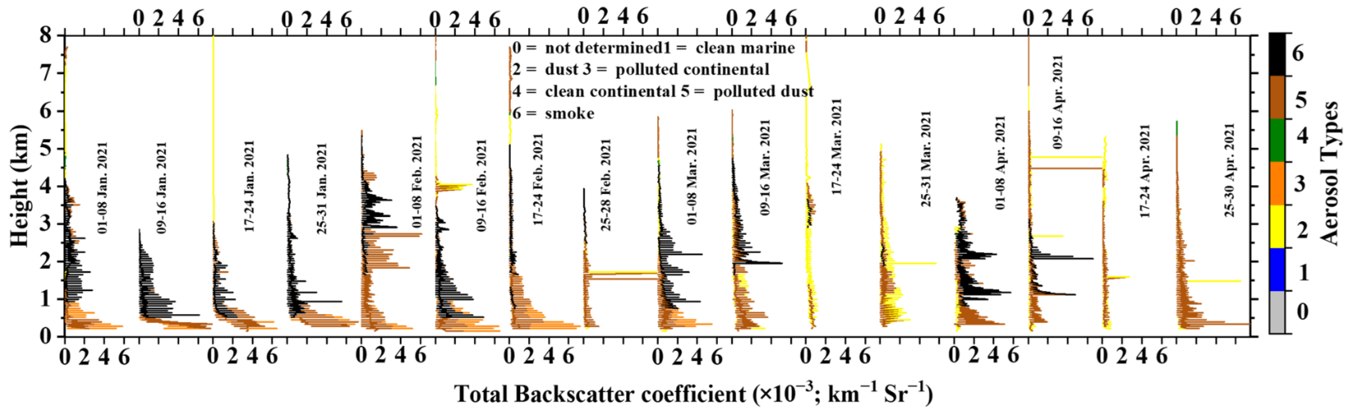
3.1. Identification of Forest Fire

India has suffered massive forest fires each year due to natural and anthropogenic causes, with the main concentration in the hilly terrains of the western/central Himalayas and the northeastern states. A large number of forest fires from November 2020 to June 2021 were reported in Odisha (51,968), Madhya Pradesh (47,795), Chhattisgarh (38,106), Maharashtra (34,025), Jharkhand (21,713), Uttarakhand (21,497), Andhra Pradesh (19,328), Telangana (18,237), Mizoram (12,864), Assam (10,718), and Manipur (10,475) [67]. Approximately 1300 hectares of forest area burned due to massive forest fires in 2021 in Uttarakhand state [68]. Based on the Forest Survey of India report of 2019, a total of 277,758 forest fire points were recorded from 2004 to 2017 across the country, and 2.56 lakh hectares of land was affected by these forest fires [69]. Figure 1 shows the forest fire counts as detected by MODIS on various days from January to April 2021. The total fire counts during January 2021 ranged from ~800 to 1690. The maximum fire counts were ~3000, 14,000, and 11,000, respectively, for February, March, and April 2021. The most affected areas during the winter months (i.e., January–February 2021) are northeast India, central India, the east coast of India, and central Indian Himalayas. However, during March–April 2021, the most commonly affected regions were the northern part of India, in addition to the dominant fires in the foothills and central Indian Himalayan region. The natural causes of forest fires are lightning, the friction of dry bamboo, stems of trees, and rolling stones. In addition to these sources, favorable atmospheric conditions, such as high atmospheric temperatures and low humidity, are more likely to lead to forest fire situations. The northern part of India is mostly affected by biomass burning. It is observed that most of the detected spots are in the Himalayan region [9,24,25,70,71], the Indo-Gangetic Plain, and the central part of the country [3,4,8,71,72].
Figure 2 shows the daily transport pathways of aerosols based on the five days backward air mass trajectories simulated by the HYSPLIT model, ending over Nainital (a high altitude remote location in the central Himalayan region) at three different altitudes (500 m, 1500 m, and 3000 m agl, respectively), as described in Section 2.1. These trajectories are color coded according to the altitude attained by the air parcel along the pathways before reaching Nainital. Figure 2 clearly indicates that the majority of the back trajectories are from the west and northwest part of the country, so the transport of dust from the Thar Desert and arid regions in the west dominates, especially during the month of March–April [73,74,75,76]. At Nainital (a high-altitude location in the central Himalayas), the air masses are not significantly affected by the majority of the fire counts, which are in the east and south directions (see Figure 1). Although several fire counts were spread over the Indian subcontinent (Figure 1) during the study period, the air masses were quickly renewed, hence indicating the low contribution of smoke to the total aerosol loading (Figure 3a).
Figure 3a shows the percentage contribution of BC aerosol optical depth to the total aerosol optical depth, which was found to be within 2% to 7%. A decreasing trend is observed in the percentage contribution of BC in the winter months from January to mid-February, whereas it stays almost constant, at around 4.5%, until mid-March. A slight drop to 3.5% is seen in March, before a further increase to 5% in April, with a decreasing trend beyond that to 2%. The percentage contribution of BC AOD was found to be above 5% during 9–31 January and 1–8 April, and to be as low as 2% at the end of April. The violin box plot of different aerosol types to the total backscatter coefficient during the fire period is shown in Figure 3b, whereas the percentage contribution of different aerosol types during January to April 2021 is shown in Figure 3c. These figures indicate that the polluted continental aerosols and the polluted dust are both contaminated or polluted by the smoke and fires, as suggested by CALIPSO vertical profiles of the total backscatter coefficient (see Figure 4; discussed later). Further, the pure dust is transported from the northwest part of the country or west Asia, as indicated by the HYSPLIT back trajectories (Figure 2). This takes into account the fact that the smoke is extremely high and is a complex mixture of continental aerosols, dust, and smoke. The pure smoke comprises more than the pure dust and pure continental aerosols, so the polluted continental aerosols and dust are indeed polluted by smoke.
Figure 4 shows the total backscatter coefficient and aerosol type variation with height. It can be observed that the aerosol content mainly comprised dust, polluted continental aerosols, polluted dust, and smoke during the period of January to April. Polluted dust was found to be a dominant aerosol subtype followed by pure smoke and dust. The presence of smoke, which polluted mostly dust and continental aerosol types during the study period, was observed at various heights, with the majority being between 0.5 and 4 km. These can be attributed to certain factors such as wildfires, industrial fires, campfires, fireplaces, and biomass burning [77].
Figure 5 shows the variation in the weekly average AOD and BC AOD at 550 nm from January to April. The mean AOD was found to vary between 0.02 and 0.04, with the maximum AOD value reaching 1.6 [78,79]. However, the AOD value was found to be 0.3 in the beginning of March, which was the lowest value during the entire study period. The AOD values in March and April were close to 0.6, indicating a high aerosol content in these summer months. A maximum AOD of 1.6 was observed during 1–8 February, 9–16 March, 25–31 March, and 9–30 April, which is also evident from Figure 3a.
The fire count was observed to be high in March and early April, as observed from Figure 1, which may have contributed to the high aerosol loading during this period. It was also observed that, during this period, there were fire counts all over India that may have contributed to the high aerosol contents. The mean BC AOD tended to vary between 0.01 and 0.03 [80], with maximum and minimum values being within the range of 0 to 0.07. A sudden dip in the value of BC AOD was observed during the beginning of March, similar to the AOD, as seen from Figure 5a. The BC AOD content was found to be high from 9 January to 25 February and 25 March to 8 April, reaching 0.7 (Figure 5b). The BC AOD contribution was also found to be the highest during this period, as observed in Figure 3a.
Figure 6 presents the weekly average maps of AOD at 550 nm over the Indian subcontinent using the dark target and deep blue combined products of MODIS Aqua and Terra Satellites. The maps are from January to April 2021, and the red dots show the MODIS fire counts. The AOD values are shown to be high all over the Indian subcontinent and vary from 0 to 1.8. The regions with lower AOD values include the northwestern part, which mainly represents the That desert and Kerala, towards the end of April. The MODIS fire counts are shown to be spread across the entire Indian subcontinent. The temporal distribution of the plots from January to April shows that the forest fires increased in intensity with the receding winter (January and February) and incoming summer season (March and April) in almost the entire Indian region [23,81,82]. However, in certain areas, such as the Thar desert in the northwestern region, forest fires were not detected, which may be because forest fires are historically infrequent in desert regions due to of the lack of a continuous fuel bed to carry a fire [83]. In the southern area, Kerala and Tamil Nadu showed no fire activity in January or April.

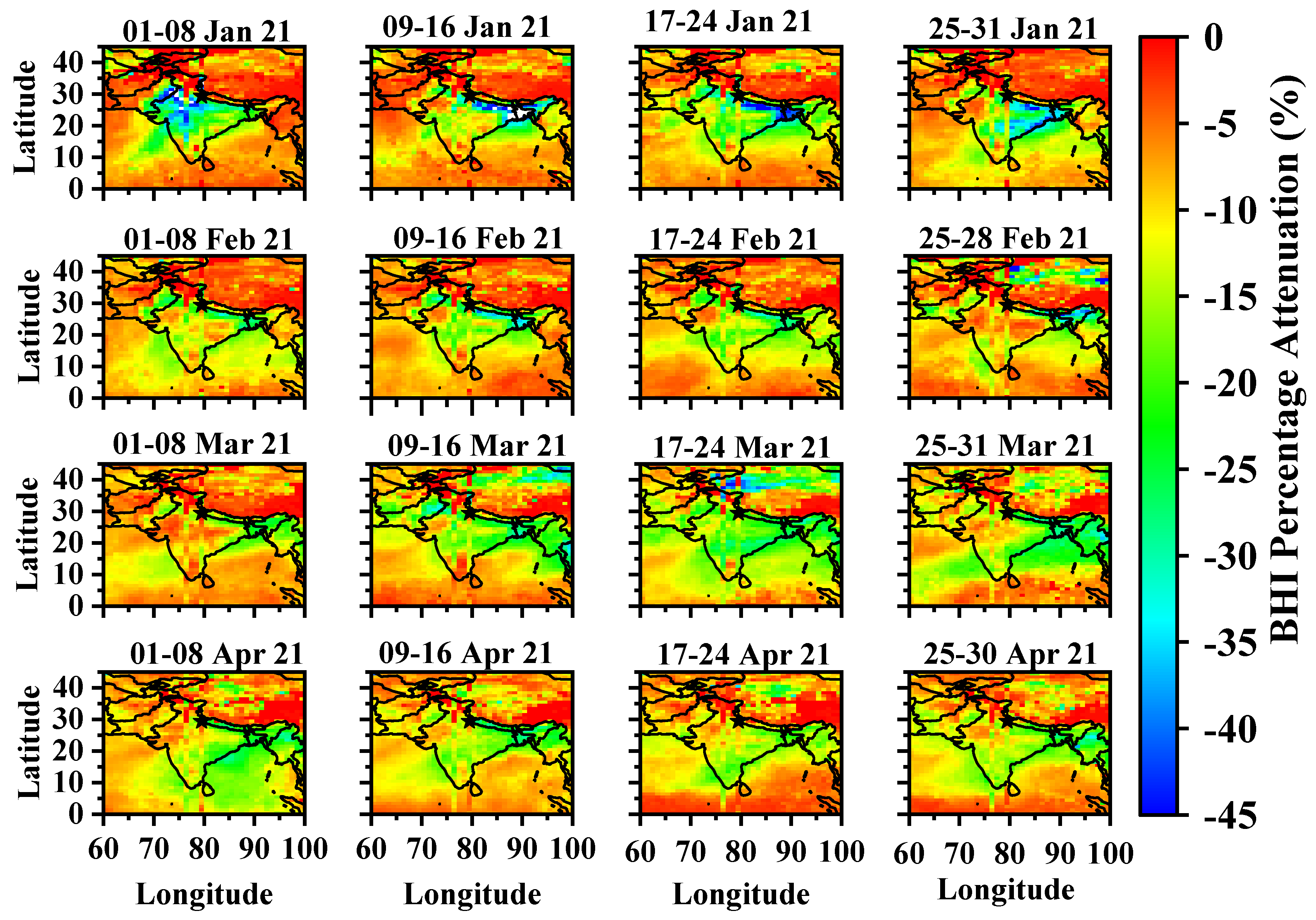
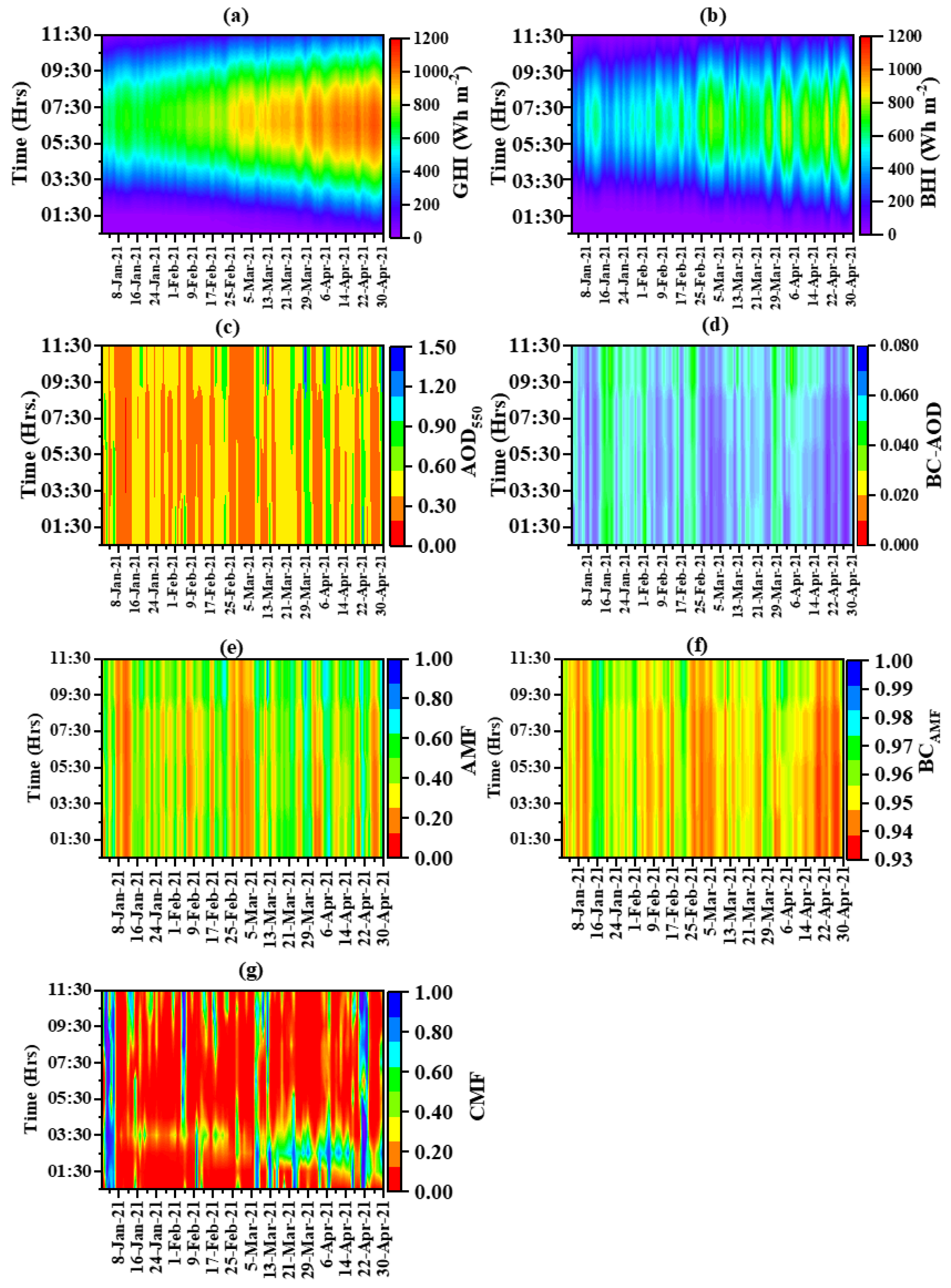
3.2. Solar Radiation Effects

Figure 7 and Figure 8 show the weekly average maps of GHI and BHI percentage attenuation, which varied from 0 to 45% during the study period. A higher percentage attenuation is shown in the Indo-Gangetic and central regions during the winter months of January and February, and can be attributed to fog cover in the northern part of the subcontinent. The months of March and April show significant reductions in GHI over all of the Indian region. A significantly higher attenuation was seen for BHI over all of the Indian subcontinent during the study period. During forest fires, the Himalayan regions and the IGP region are impacted by the outflow of pollutants [84]. Forest fire behavior is governed by interactions at different temporal and spatial scales, as shown in Figure 6, which tend to affect the GHI and BHI levels, as shown in Figure 7 and Figure 8 [85]. The GHI percentage attenuation was high during the winter month of January, mostly in the northern part of the subcontinent. This may be attributed to fog cover and aerosol content. Another probable reason may be the forest fire in the Himalayan region and Indo-Gangetic plains, and the eastern part of the region, as shown in Figure 6. The BHI percentage attenuation, which was as high as 45%, was seen in several regions in January, mainly around the western region, the Indo-Gangetic plains, and some of the eastern areas, and gradually increased with the onset of the summer season until April.
Figure 9 shows the variation in GHI, BHI, AOD, BC AOD, AMF, BC AMF, and CMF as a function of the day and time of the day from January to April. Figure 9a shows that the intensity of GHI increased from January to April, indicating the shift from winter to summer months. The GHI values are shown to be low in the morning and evening hours, and to reach a maximum around noon (that is, 06:30 UTC for the Indian region), during which the GHI reached 1200 Wh/m2 in March and April. The BHI values, as shown in Figure 9b, do not follow a set pattern unlike in the case of GHI, but vary with a large amount of fluctuation from January to April, with a maximum value of 700 Wh/m2. Figure 9c shows the variation of AOD at 550 nm, and indicates the variation in AOD was mostly between 0.2 and 0.4 throughout the day, although AOD also reached values up to 1.5 on some days. A value as high as 1.5 is seen mostly in the evening hours. Figure 9d presents the variation of BC AOD, which was found to vary within 0.04 during the daytime. The AMF, as shown in Figure 9e, was found to vary from 0 to 0.6 during most days, with a few days showing values even reaching up to 1. Figure 9f shows the BC AMF, whose value was found to vary from 0.93 to 0.97 in most of the cases. The variation in CMF, as shown in Figure 9g, was found to vary from 0 to 1, where 0 indicates a cloudless scenario. The early days of January experienced heavy cloud cover throughout the daytime. The CMF is shown to be in the range of 0.4 to 0.7 during the morning hours of March and April.
Figure 10 shows the time-series plots of GHI, BHI, and AOD at 550 nm during the study period. The AOD values are shown to vary in the range of 0.2 to 0.9. There were fluctuations in the AOD during the study period, especially during March and April. The GHI-based energy production is shown to increase more linearly, from 3500 to 8500 kWh from the winter month of January to the summer month of April. During January, the GHI values were within 5000 kWh, and in February it reached 5500 kWh. The summer months of March and April showed a much higher GHI energy, of between 6000 and 8000 kWh. However, the energy contribution from BHI increased abruptly during the same period, with huge fluctuations between 2000 and 6500 kWh.
Figure 11a shows the time-series plots of aerosol and cloud modification fractions during the study period. The aerosol modification fraction was found to vary between 0.4 and 0.9, whereas the cloud modification fraction varied between 0.1 and 1. The AMF values varied in the range of 0.5 to 0.7 in January and February, with a few values reaching 0.8 at the beginning of January and towards the end of February. The months of March and April had AMF values in the range from 0.4 to 0.8. The CMF values were found to vary between 0.8 and 1 in January and February, with some values going below 0.8 and a few values as low as 0.1. The values in March and April are shown to vary between 0.4 and 1, with some values going below 0.4 and some as low as 0.2.
The frequency distribution of AMF and CMF from January to April is depicted in Figure 11b. The variation was found to be from 0 to 25% for AMF and 55% for CMF. It can be observed that the AMF values were dominated by values ranging between 0.5 to 0.8 [36], which indicate heavy aerosol content during these months. The frequency of occurrence of AMF was highest in the range of 0.5 to 0.8, and was within 5% for other values. However, the frequency of occurrence of CMF values was found to be within 10% for all values varying from 0 to 0.9, with the exception of 1, which had a frequency of occurrence of 55%. This indicates that most of the days were cloud-free during this period.

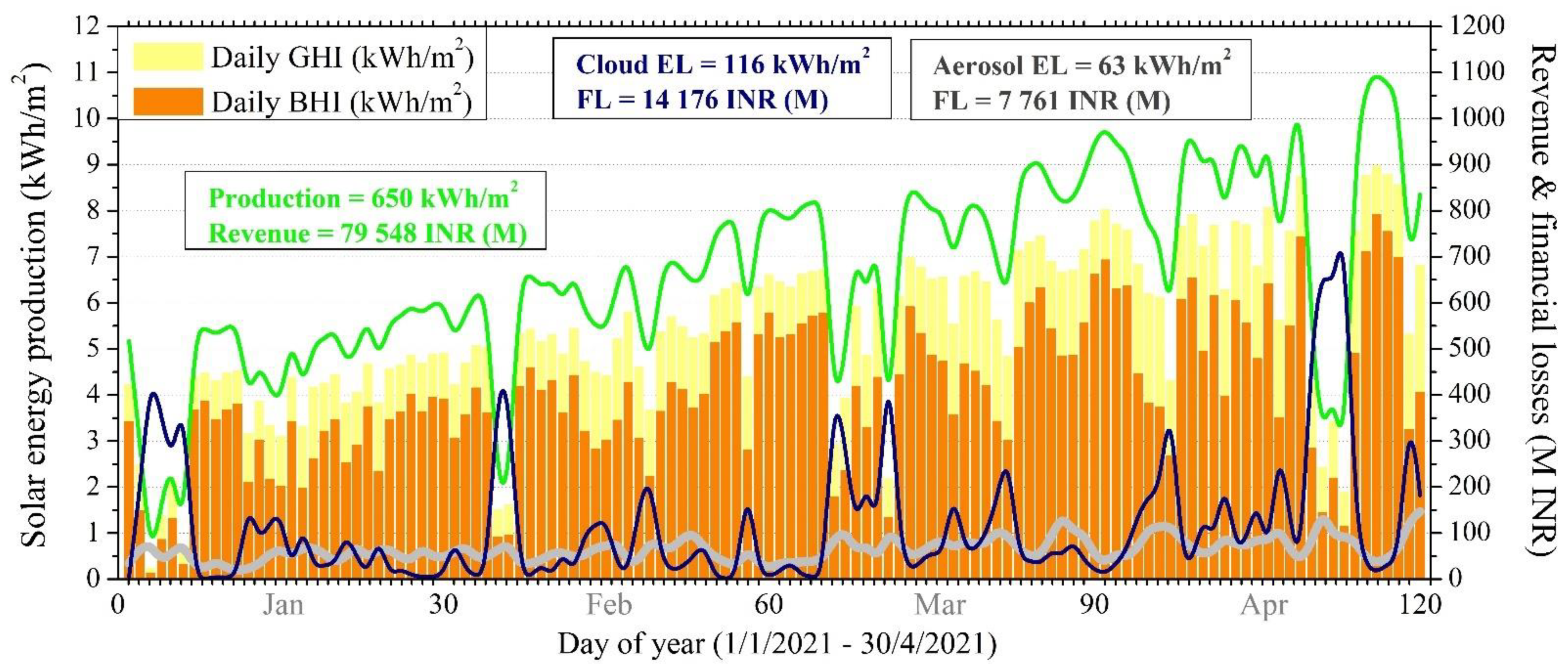
3.3. Solar Energy Effects

Figure 12 represents the time-series plots of percentage attenuation of GHI and BHI in the presence of aerosols, black carbon, and clouds. In general, significantly more fluctuations were found in the case of BHI than in that of GHI, as BHI is the scattered component that is severely impacted by the atmospheric constituents. The GHI percentage attenuation was found to be well within 10% and that in the case of BC was mostly within 1%. Moreover, in the presence of clouds, the fluctuations in the percentage attenuation were greater and reached 40%. The BHI percentage attenuation in the presence of black carbon was found to be within 4%, whereas it reached 20% in the case of aerosols. Clouds were found to severely impact the BHI, with percentage attenuation reaching 40%. This is because the diffuse fraction of the radiation increases due to scattering of the incoming radiation in several directions other than the incidence direction [37,63,86].
Figure 13 presents the variation in GHI and BHI under different atmospheric conditions from January to April. It is shown that the GHI and BHI values under clear sky conditions increased almost linearly with the days varying from the winter month of January to the summer month of April. A similar trend can be observed for the case of black carbon, which did not have a significant impact on GHI and BHI. However, fluctuations can be seen in the case of aerosols and clouds. The presence of aerosols in the atmosphere caused fluctuations in GHI and BHI. These fluctuations can be observed to be less during the winter months, whereas the fluctuations tended to be enhanced during April. The presence of clouds clearly increased the fluctuations in GHI and BHI, as shown in Figure 13g,d, respectively. The fluctuations induced by the presence of clouds and aerosols were pronounced during the entire period. Figure 13a shows that the GHI under clear sky conditions varied between 200 and 400 W/m2, with a minimum value of 200 W/m2 at the beginning of January and a maximum value of 400 W/m2 towards the end of April. Similarly, Figure 13b shows that the BHI values varied between a minimum value of 200 W/m2 at the beginning of January and a maximum value of 400 W/m2 towards the end of April. Figure 13c shows that GHI values considering the effect of aerosols varied from 150 to 350 W/m2. The BHI in the presence of aerosols showed slightly more fluctuations than GHI, with a variation from 100 to 300 W/m2, as shown in Figure 13d.
Figure 13e,f shows the GHI and BHI variations in the presence of black carbon, and it can be observed that the variation was similar to that of the clear sky condition shown in Figure 13a,b. This indicates that black carbon does not have a very significant impact on GHI and BHI compared to other atmospheric components such as aerosols and clouds [87,88]. The combined effect of clouds and aerosols is shown in Figure 13g,h. The GHI, in this case, is shown to vary between 0 and 350 W/m2, and BHI varied from 0 to 300 W/m2, with significantly more fluctuations than shown in Figure 13c,d, thus indicating the strong effect of clouds on irradiances.
Finally, Figure 14 presents the financial analysis of the impact of clouds and aerosols on the solar energy production, which was quantified in terms of daily mean and total energy losses (EL), financial losses (FL), and solar energy potential following the methodology given elsewhere [36,39,65]. The figure refers to the total solar energy production in India, which is 40 GW, and the results are generalized for the solar plant production of the whole country. The total solar energy production during the study period was found to be 650 kWh/m2. The daily solar energy production increased to 9 kWh/m2 for GHI and 8 W/m2 for BHI, with a slight linear increase from January to April. There were dips in energy production at the beginning of January and February, and towards the end of April. The energy loss due to the presence of clouds was found to be 116 kWh/m2, whereas it was about 63 kWh/m2 in the presence of the aerosols. The losses due to aerosols seem to be within 2 kWh/m2, whereas in the case of clouds, the losses reached 7 kWh/m2. The revenue generated from solar energy utilization is about INR 79,548 million. The financial loss was found to vary within 1.5 kWh/m2 in the presence of aerosols and 700 kWh/m2 in the presence of clouds. The daily financial loss due to the presence of clouds was found to be high during the beginning of January and February, reaching INR 400 million, and increased to INR 700 million towards the end of April. This analysis of daily energy and financial losses can help grid operators to plan and schedule power generation and supply. A similar analysis was also presented in several earlier papers [36,39,89] for the climatological conditions of India, which showed the percentage variation between the maximum and minimum yield to be around 40%. In previous works [90,91], the authors showed that detailed observations of the types of aerosol, their horizontal and vertical distribution, and appropriate and more detailed measurements of atmospheric parameters, can reduce the uncertainties in the radiative effects of clouds and aerosols.

4. Conclusions

The present study was the first attempt to study the impact of massive forest fires on solar energy production over the Indian subcontinent via remote sensing techniques. For this purpose, we exploited the Earth observation data and techniques in terms of passive and active remote sensing, in conjunction with model simulations, in order to provide a realistic representation of the atmospheric effects on solar energy production during the period of the fires.
The high AOD values (up to 1.8) during the massive forest fire events led to attenuation of GHI and BHI of ~0 to 45%. The air masses were renewed quickly, thus mitigating the smoke contribution to the total aerosol loads, which were dominated by continental pollution. By comparison, the clouds continued to be the prevailing attenuator for solar irradiation, followed by aerosols (almost 50% of the cloud effect), resulting in financial losses for total PV production at the country scale of INR 14.2 and 7.8 million, respectively. In a region where the continental aerosols and dust are the most frequent aerosol sources, smoke polluted these sources, thus minimizing the clean continental aerosols to 1.5%. This highlights that smoke is the highest pure aerosol source (21.2%), followed by dust (11.3%), which comes from the northwest. The remaining smoke aerosols contributed to the continental and dust aerosols, increasing their percentages to 48.8% and 17.3%, respectively.
This analysis of daily energy and financial losses due to the direct and indirect effects of forest fires on the production of solar plants can help grid operators to plan and schedule power generation, and in the distribution, supply, security, and overall stability of power production. The findings of the present study will drastically increase the awareness among decision makers regarding the effect of forest fires on energy management and planning at a country level. In addition, this research will support the mitigation processes and policies for climate change and its direct and indirect impacts on sustainable development.

Author Contributions

U.C.D.: designed, conceptualized the idea for this study, methodology, data curation, and plotting, writing original draft, revised, reviewing. P.G.K.: data curation and methodology, conceptualization, discussion, revised, reviewing and editing. R.S.: data curation and plotting. P.N.P.: data curation, methodology, writing. All authors have read and agreed to the published version of the manuscript.

Funding

The current research has not received any external funding.

Institutional Review Board Statement

Not applicable.

Informed Consent Statement

Not applicable.

Data Availability Statement

Data can be available after request.

Acknowledgments

Umesh Chandra Dumka thanks Director (Dipankar Banerjee) ARIES, Nainital for his encouragement and continuous support of this study. The analysis and visualizations used in the current study were produced by the Giovanni online data system, developed and maintained by the NASA GES DISC, and is highly acknowledged. We would like to acknowledge the use of data or images from NASA’s Fire Information for Resource Management System (FIRMS; https://earthdata.nasa.gov/firms (last assessed on 1 October 2021)), part of NASA’s Earth Observing System Data and Information System (EOSDIS). We acknowledge the CALIPSO Lidar Science team, the data management team, and the atmospheric science data center at NASA Langley Research Center for archiving the CALIPSO data. We thank Akriti Masoom for fruitful discussion to finalize the paper. Umesh Chandra Dumka thanks Dimitris G Kaskaoutis for his valuable support and fruitful discussion to finalize the current paper. Panagiotis G. Kosmopoulos acknowledges the EuroGEO e-shape project under the grant agreement 820852, along with the Excelsior project under the grant agreement 857510 and the Eiffel project under grant agreement 101003518. We thank the editors Cicily Chen and Irelia Wang and three anonymous reviewers for providing insightful comments and valuable suggestions, which helped us to improve the scientific quality of the manuscript.

Conflicts of Interest

The authors declare no conflict of interest.

References

  1. Vadrevu, K.P.; Lasko, K.; Giglio, L.; Schroeder, W.; Biswas, S.; Justice, C. Trends in Vegetation fires in South and Southeast Asian Countries. Sci. Rep. 2019, 9, 7422. [Google Scholar] [CrossRef] [PubMed]
  2. Ciccioli, P.; Centritto, M.; Loreto, F. Biogenic volatile organic compound emissions from vegetation fires. Plant Cell Environ. 2014, 37, 1810–1825. [Google Scholar] [CrossRef] [PubMed] [Green Version]
  3. Jethva, H.; Torres, O.; Field, R.D.; Lyapustin, A.; Gautam, R.; Kayetha, V. Connecting Crop Productivity, Residue Fires, and Air Quality over Northern India. Sci. Rep. 2019, 9, 16594. [Google Scholar] [CrossRef] [PubMed] [Green Version]
  4. Jethva, H.; Chand, D.; Torres, O.; Gupta, P.; Lyapustin, A.; Patadia, F. Agricultural burning and air quality over northern india: A synergistic analysis using nasa’s a-train satellite data and ground measurements. Aerosol Air Qual. Res. 2018, 18, 1756–1773. [Google Scholar] [CrossRef] [Green Version]
  5. Van Leeuwen, T.T.; Van Der Werf, G.R. Spatial and temporal variability in the ratio of trace gases emitted from biomass burning. Atmos. Chem. Phys. 2011, 11, 3611–3629. [Google Scholar] [CrossRef] [Green Version]
  6. Pani, S.K.; Lin, N.H.; Chantara, S.; Wang, S.H.; Khamkaew, C.; Prapamontol, T.; Janjai, S. Radiative response of biomass-burning aerosols over an urban atmosphere in northern peninsular Southeast Asia. Sci. Total Environ. 2018, 633, 892–911. [Google Scholar] [CrossRef] [PubMed]
  7. Van Der Werf, G.R.; Randerson, J.T.; Giglio, L.; Collatz, G.J.; Mu, M.; Kasibhatla, P.S.; Morton, D.C.; Defries, R.S.; Jin, Y.; Van Leeuwen, T.T. Global fire emissions and the contribution of deforestation, savanna, forest, agricultural, and peat fires (1997–2009). Atmos. Chem. Phys. 2010, 10, 11707–11735. [Google Scholar] [CrossRef] [Green Version]
  8. Kaskaoutis, D.G.; Kumar, S.; Sharma, D.; Singh, R.P.; Kharol, S.K.; Sharma, M.; Singh, A.K.; Singh, S.; Singh, A.; Singh, D. Effects of crop residue burning on aerosol properties, plume characteristics, and long-range transport over northern India. J. Geophys. Res. 2014, 119, 5424–5444. [Google Scholar] [CrossRef]
  9. Kumar, R.; Naja, M.; Satheesh, S.K.; Ojha, N.; Joshi, H.; Sarangi, T.; Pant, P.; Dumka, U.C.; Hegde, P.; Venkataramani, S. Influences of the springtime northern Indian biomass burning over the central Himalayas. J. Geophys. Res. Atmos. 2011, 116, D19302. [Google Scholar] [CrossRef]
  10. Vadrevu, K.P.; Lasko, K.; Giglio, L.; Justice, C. Vegetation fires, absorbing aerosols and smoke plume characteristics in diverse biomass burning regions of Asia. Environ. Res. Lett. 2015, 10, 105003. [Google Scholar] [CrossRef] [Green Version]
  11. Wang, Y.; Zhang, Q.Q.; He, K.; Zhang, Q.; Chai, L. Sulfate-nitrate-ammonium aerosols over China: Response to 2000–2015 emission changes of sulfur dioxide, nitrogen oxides, and ammonia. Atmos. Chem. Phys. 2013, 13, 2635–2652. [Google Scholar] [CrossRef] [Green Version]
  12. Zhang, H.; Hu, D.; Chen, J.; Ye, X.; Wang, S.X.; Hao, J.M.; Wang, L.; Zhang, R.; An, Z. Particle size distribution and polycyclic aromatic hydrocarbons emissions from agricultural crop residue burning. Environ. Sci. Technol. 2011, 45, 5477–5482. [Google Scholar] [CrossRef] [PubMed]
  13. Ramanathan, V.; Carmichael, G. Global and regional climate changes due to black carbon. Nat. Geosci. 2008, 1, 221–227. [Google Scholar] [CrossRef]
  14. Singh, P.; Roy, A.; Bhasin, D.; Kapoor, M.; Ravi, S.; Dey, S. Crop Fires and Cardiovascular Health—A Study from North India. SSM Popul. Health 2021, 14, 100757. [Google Scholar] [CrossRef] [PubMed]
  15. Vinjamuri, K.S.; Mhawish, A.; Banerjee, T.; Sorek-Hamer, M.; Broday, D.M.; Mall, R.K.; Latif, M.T. Vertical distribution of smoke aerosols over upper Indo-Gangetic Plain. Environ. Pollut. 2020, 257, 113377. [Google Scholar] [CrossRef]
  16. Adam, M.; Stachlewska, I.S.; Mona, L.; Papagiannopoulos, N.; Antonio, J.; Sicard, M.; Nicolae, D.; Belegante, L.; Janicka, L.; Alados-arboledas, L.; et al. Biomass burning events measured by lidars in EARLINET—Part 2: Optical properties investigation. Atmos. Chem. Phys. Discuss. 2021. [Google Scholar] [CrossRef]
  17. Adam, M.; Nicolae, D.; Stachlewska, I.S.; Papayannis, A.; Balis, D. Biomass burning events measured by lidars in EARLINE—Part 1: Data analysis methodology. Atmos. Chem. Phys. 2020, 20, 13905–13927. [Google Scholar] [CrossRef]
  18. Adam, M.G.; Chiang, A.W.J.; Balasubramanian, R. Insights into characteristics of light absorbing carbonaceous aerosols over an urban location in Southeast Asia. Environ. Pollut. 2020, 257, 113425. [Google Scholar] [CrossRef]
  19. Chavan, P.; Fadnavis, S.; Chakroborty, T.; Sioris, C.E.; Griessbach, S.; Müller, R. The outflow of Asian biomass burning carbonaceous aerosol into the upper troposphere and lower stratosphere in spring: Radiative effects seen in a global model. Atmos. Chem. Phys. 2021, 21, 14371–14384. [Google Scholar] [CrossRef]
  20. Kalita, G.; Kunchala, R.K.; Fadnavis, S.; Kaskaoutis, D.G. Long term variability of carbonaceous aerosols over Southeast Asia via reanalysis: Association with changes in vegetation cover and biomass burning. Atmos. Res. 2020, 245, 105064. [Google Scholar] [CrossRef]
  21. Saxena, P.; Sonwani, S.; Srivastava, A.; Jain, M.; Srivastava, A.; Bharti, A.; Rangra, D.; Mongia, N.; Tejan, S.; Bhardwaj, S. Impact of crop residue burning in Haryana on the air quality of Delhi, India. Heliyon 2021, 7, e06973. [Google Scholar] [CrossRef] [PubMed]
  22. Sarkar, S.; Singh, R.P.; Chauhan, A. Crop Residue Burning in Northern India: Increasing Threat to Greater India. J. Geophys. Res. Atmos. 2018, 123, 6920–6934. [Google Scholar] [CrossRef] [Green Version]
  23. Singh, P.; Dey, S. Crop burning and forest fires: Long-term effect on adolescent height in India. Resour. Energy Econ. 2021, 65, 101244. [Google Scholar] [CrossRef]
  24. Bali, K.; Mishra, A.K.; Singh, S. Impact of anomalous forest fire on aerosol radiative forcing and snow cover over Himalayan region. Atmos. Environ. 2017, 150, 264–275. [Google Scholar] [CrossRef]
  25. Kumar, A.; Bali, K.; Singh, S.; Naja, M.; Mishra, A.K. Estimates of reactive trace gases (NMVOCs, CO and NOx) and their ozone forming potentials during forest fire over Southern Himalayan region. Atmos. Res. 2019, 227, 41–51. [Google Scholar] [CrossRef]
  26. Casagrande, M.S.G.; Martins, F.R.; Rosário, N.E.; Lima, F.J.L.; Gonçalves, A.R.; Costa, R.S.; Zarzur, M.; Pes, M.P.; Pereira, E.B. Numerical assessment of downward incoming solar irradiance in smoke influenced regions—A case study in brazilian amazon and cerrado. Remote Sens. 2021, 13, 4527. [Google Scholar] [CrossRef]
  27. Piedra, P.G.; Llanza, L.R.; Moosmüller, H. Optical losses of photovoltaic modules due to mineral dust deposition: Experimental measurements and theoretical modeling. Sol. Energy 2018, 164, 160–173. [Google Scholar] [CrossRef]
  28. Sayyah, A.; Horenstein, M.N.; Mazumder, M.K. Energy yield loss caused by dust deposition on photovoltaic panels. Sol. Energy 2014, 107, 576–604. [Google Scholar] [CrossRef]
  29. Sulaiman, S.A.; Singh, A.K.; Mokhtar, M.M.M.; Bou-Rabee, M.A. Influence of dirt accumulation on performance of PV panels. Energy Procedia 2014, 50, 50–56. [Google Scholar] [CrossRef] [Green Version]
  30. Zabeltitz, C.H.R.V.O.N. Effective Use of Renewable Energies for Greenhouse Heating. Renew. Energy 1994, 5, 479–485. [Google Scholar] [CrossRef]
  31. Ahmed, R.; Sreeram, V.; Mishra, Y.; Arif, M.D. A review and evaluation of the state-of-the-art in PV solar power forecasting: Techniques and optimization. Renew. Sustain. Energy Rev. 2020, 124, 109792. [Google Scholar] [CrossRef]
  32. Guo, Z.; Zhou, K.; Zhang, C.; Lu, X.; Chen, W.; Yang, S. Residential electricity consumption behavior: Influencing factors, related theories and intervention strategies. Renew. Sustain. Energy Rev. 2018, 81, 399–412. [Google Scholar] [CrossRef]
  33. Mocanu, E.; Nguyen, P.H.; Gibescu, M.; Kling, W.L. Deep learning for estimating building energy consumption. Sustain. Energy Grids Netw. 2016, 6, 91–99. [Google Scholar] [CrossRef]
  34. IEA. Solar Energy: Maping the Road Ahead; IEA: Paris, France, 2019; Volume 20. [Google Scholar]
  35. Charles Rajesh Kumar, J.; Majid, M.A. Renewable energy for sustainable development in India: Current status, future prospects, challenges, employment, and investment opportunities. Energy. Sustain. Soc. 2020, 10, 1–36. [Google Scholar] [CrossRef]
  36. Dumka, U.C.; Kosmopoulos, P.G.; Ningombam, S.S.; Masoom, A. Impact of aerosol and cloud on the solar energy potential over the central gangetic himalayan region. Remote Sens. 2021, 13, 3248. [Google Scholar] [CrossRef]
  37. Masoom, A.; Kosmopoulos, P.; Bansal, A.; Gkikas, A. Forecasting dust impact on solar energy using remote sensing and modeling techniques. Sol. Energy 2021, 228, 317–332. [Google Scholar] [CrossRef]
  38. Masoom, A.; Kosmopoulos, P.; Bansal, A.; Kazadzis, S. Solar energy estimations in india using remote sensing technologies and validation with sun photometers in urban areas. Remote Sens. 2020, 12, 254. [Google Scholar] [CrossRef] [Green Version]
  39. Masoom, A.; Kosmopoulos, P.; Kashyap, Y.; Kumar, S.; Bansal, A. Rooftop photovoltaic energy production management in india using earth-observation data and modeling techniques. Remote Sens. 2020, 12, 1921. [Google Scholar] [CrossRef]
  40. Rolph, G.; Stein, A.; Stunder, B. Real-time Environmental Applications and Display sYstem: READY. Environ. Model. Softw. 2017, 95, 210–228. [Google Scholar] [CrossRef]
  41. Stein, A.F.; Draxler, R.R.; Rolph, G.D.; Stunder, B.J.B.; Cohen, M.D.; Ngan, F. Noaa’s hysplit atmospheric transport and dispersion modeling system. Bull. Am. Meteorol. Soc. 2015, 96, 2059–2077. [Google Scholar] [CrossRef]
  42. Inness, A.; Ades, M.; Agustí-Panareda, A.; Barr, J.; Benedictow, A.; Blechschmidt, A.M.; Jose Dominguez, J.; Engelen, R.; Eskes, H.; Flemming, J.; et al. The CAMS reanalysis of atmospheric composition. Atmos. Chem. Phys. 2019, 19, 3515–3556. [Google Scholar] [CrossRef] [Green Version]
  43. Morcrette, J.J.; Boucher, O.; Jones, L.; Salmond, D.; Bechtold, P.; Beljaars, A.; Benedetti, A.; Bonet, A.; Kaiser, J.W.; Razinger, M.; et al. Aerosol analysis and forecast in the european centre for medium-range weather forecasts integrated forecast system: Forward modeling. J. Geophys. Res. Atmos. 2009, 114, D06206. [Google Scholar] [CrossRef]
  44. Bozzo, A.; Remy, S.; Benedetti, A.; Flemming, J.; Bechtold, P.; Rodwell, M.J.; Morcrette, J.-J. Implementation of a CAMS-Based Aerosol Climatology in the IFS; Its Technical memorandum; ECMWF: Reading, UK, 2017; pp. 1–35. [Google Scholar]
  45. Hogan, R.J.; Bozzo, A. ECRAD: A new radiation scheme for the IFS. ECMWF Tech. 2016, 787, 1–33. [Google Scholar]
  46. Bilal, M.; Mhawish, A.; Nichol, J.E.; Qiu, Z.; Nazeer, M.; Ali, M.A.; de Leeuw, G.; Levy, R.C.; Wang, Y.; Chen, Y.; et al. Air pollution scenario over Pakistan: Characterization and ranking of extremely polluted cities using long-term concentrations of aerosols and trace gases. Remote Sens. Environ. 2021, 264, 112617. [Google Scholar] [CrossRef]
  47. Flemming, J.; Benedetti, A.; Inness, A.; Engelen J, R.; Jones, L.; Huijnen, V.; Remy, S.; Parrington, M.; Suttie, M.; Bozzo, A.; et al. The CAMS interim Reanalysis of Carbon Monoxide, Ozone and Aerosol for 2003–2015. Atmos. Chem. Phys. 2017, 17, 1945–1983. [Google Scholar] [CrossRef] [Green Version]
  48. Mohammadpour, K.; Sciortino, M.; Kaskaoutis, D.G. Classification of weather clusters over the Middle East associated with high atmospheric dust-AODs in West Iran. Atmos. Res. 2021, 259, 105682. [Google Scholar] [CrossRef]
  49. Salamalikis, V.; Vamvakas, I.; Blanc, P.; Kazantzidis, A. Ground-based validation of aerosol optical depth from CAMS reanalysis project: An uncertainty input on direct normal irradiance under cloud-free conditions. Renew. Energy 2021, 170, 847–857. [Google Scholar] [CrossRef]
  50. Hsu, N.C.; Jeong, M.J.; Bettenhausen, C.; Sayer, A.M.; Hansell, R.; Seftor, C.S.; Huang, J.; Tsay, S.C. Enhanced Deep Blue aerosol retrieval algorithm: The second generation. J. Geophys. Res. Atmos. 2013, 118, 9296–9315. [Google Scholar] [CrossRef]
  51. Levy, R.C.; Mattoo, S.; Munchak, L.A.; Remer, L.A.; Sayer, A.M.; Patadia, F.; Hsu, N.C. The Collection 6 MODIS aerosol products over land and ocean. Atmos. Meas. Tech. 2013, 6, 2989–3034. [Google Scholar] [CrossRef] [Green Version]
  52. Levy, R.C.; Remer, L.A.; Kleidman, R.G.; Mattoo, S.; Ichoku, C.; Kahn, R.; Eck, T.F. Global evaluation of the Collection 5 MODIS dark-target aerosol products over land. Atmos. Chem. Phys. 2010, 10, 10399–10420. [Google Scholar] [CrossRef] [Green Version]
  53. Giglio, L.; Schroeder, W.; Justice, C.O. The collection 6 MODIS active fire detection algorithm and fire products. Remote Sens. Environ. 2016, 178, 31–41. [Google Scholar] [CrossRef] [PubMed] [Green Version]
  54. Giglio, L.; Descloitres, J.; Justice, C.O.; Kaufman, Y.J. An enhanced contextual fire detection algorithm for MODIS. Remote Sens. Environ. 2003, 87, 273–282. [Google Scholar] [CrossRef]
  55. Ningombam, S.S.; Dumka, U.C.; Srivastava, A.K.; Song, H.J. Optical and physical properties of aerosols during active fire events occurring in the Indo-Gangetic Plains: Implications for aerosol radiative forcing. Atmos. Environ. 2020, 223, 117225. [Google Scholar] [CrossRef]
  56. Winker, D.M.; Hunt, W.H.; McGill, M.J. Initial performance assessment of CALIOP. Geophys. Res. Lett. 2007, 34, 1–5. [Google Scholar] [CrossRef] [Green Version]
  57. Young, S.A.; Vaughan, M.A. The retrieval of profiles of particulate extinction from cloud-aerosol lidar infrared pathfinder satellite observations (CALIPSO) data: Algorithm description. J. Atmos. Ocean. Technol. 2009, 26, 1105–1119. [Google Scholar] [CrossRef]
  58. Vaughan, M.; Pitts, M.; Trepte, C.; Winker, D.; Detweiler, P.; Garnier, A.; Getzewich, B.; Hunt, W.; Lambeth, J.; Lee, K.-P.; et al. Cloud–Aerosol LIDAR Infrared Pathfinder Satellite Observations (CALIPSO) Data Management System Data Products Catalog; NASA: Washington, DC, USA, 2018.
  59. Huang, J.; Guo, J.; Wang, F.; Liu, Z.; Jeong, M.J.; Yu, H.; Zhang, Z. CALIPSO inferred most probable heights of global dust and smoke layers. J. Geophys. Res. 2015, 120, 5085–5100. [Google Scholar] [CrossRef]
  60. MétéoFrance. Algorithm Theoretical Basis Document for Cloud Products (CMa-PGE01 v3.2, CT-PGE02 v2.2 & CTTH-PGE03 v2.2); Technical Report SAF/NWC/CDOP/MFL/SCI/ATBD/01; MétéoFrance: Paris, France, 2013. [Google Scholar]
  61. Emde, C.; Buras-Schnell, R.; Kylling, A.; Mayer, B.; Gasteiger, J.; Hamann, U.; Kylling, J.; Richter, B.; Pause, C.; Dowling, T.; et al. The libRadtran software package for radiative transfer calculations (version 2.0.1). Geosci. Model Dev. 2016, 9, 1647–1672. [Google Scholar] [CrossRef] [Green Version]
  62. Mayer, B.; Kylling, A. Technical note: The libRadtran software package for radiative transfer calculations—Description and examples of use. Atmos. Chem. Phys. 2005, 5, 1855–1877. [Google Scholar] [CrossRef] [Green Version]
  63. Kosmopoulos, P.G.; Kazadzis, S.; Taylor, M.; Raptis, P.I.; Keramitsoglou, I.; Kiranoudis, C.; Bais, A.F. Assessment of surface solar irradiance derived from real-time modelling techniques and verification with ground-based measurements. Atmos. Meas. Tech. 2018, 11, 907–924. [Google Scholar] [CrossRef] [Green Version]
  64. Ricchiazzi, P.; Yang, S.; Gautier, C.; Sowle, D. SBDART: A Research and Teaching Software Tool for Plane-Parallel Radiative Transfer in the Earth’s Atmosphere. Bull. Am. Meteorol. Soc. 1998, 79, 2101–2114. [Google Scholar] [CrossRef] [Green Version]
  65. Kosmopoulos, P.G.; Kazadzis, S.; El-Askary, H.; Taylor, M.; Gkikas, A.; Proestakis, E.; Kontoes, C.; El-Khayat, M.M. Earth-observation-based estimation and forecasting of particulate matter impact on solar energy in Egypt. Remote Sens. 2018, 10, 1870. [Google Scholar] [CrossRef] [Green Version]
  66. Shettle, E.P. Models of Aerosols, Clouds, and Precipitation for Atmospheric Propagation Studies. In Proceedings of the Atmospheric Propagation in the UV, Visible, IR and MM Wave Region and Related Systems Aspects, Copenhagen, Denmark, 9–13 October 1989. [Google Scholar]
  67. Senapati, A. Odisha Recorded the Most Forest Fires in India Last Season. Down to Earth. pp. 1–16. Available online: https://www.downtoearth.org.in/news/environment/odisha-recorded-the-most-forest-fires-in-india-last-season-78129 (accessed on 27 July 2021).
  68. Sajwan, R.; Singh, M. Climate Change Is Real: Six Months on, Uttarakhand Forests Still Ablaze. Down to Earth. pp. 1–10. Available online: https://www.downtoearth.org.in/news/climate-change/climate-change-is-real-six-months-on-uttarakhand-forests-still-ablaze-76318 (accessed on 6 April 2021).
  69. Alam, M. India Has Already Witnessed 3 Big Forest Fires in 2021, Odisha’s Simlipal National Park Latest to Fall Prey. 2021, pp. 6–11. Available online: https://www.news18.com/news/india/india-has-already-witnessed-3-big-forest-fires-in-2021-odishas-simlipal-national-park-latest-to-fall-prey-3529265.html (accessed on 13 March 2021).
  70. Vadrevu, K.P.; Ellicott, E.; Giglio, L.; Badarinath, K.V.S.; Vermote, E.; Justice, C.; Lau, W.K.M. Vegetation fires in the himalayan region—Aerosol load, black carbon emissions and smoke plume heights. Atmos. Environ. 2012, 47, 241–251. [Google Scholar] [CrossRef]
  71. Vadrevu, K.P.; Ellicott, E.; Badarinath, K.V.S.; Vermote, E. MODIS derived fire characteristics and aerosol optical depth variations during the agricultural residue burning season, north India. Environ. Pollut. 2011, 159, 1560–1569. [Google Scholar] [CrossRef] [PubMed]
  72. Vadrevu, K.P.; Giglio, L.; Justice, C. Satellite based analysis of fire-carbon monoxide relationships from forest and agricultural residue burning (2003–2011). Atmos. Environ. 2013, 64, 179–191. [Google Scholar] [CrossRef]
  73. Dumka, U.C.; Kaskaoutis, D.G.; Francis, D.; Chaboureau, J.P.; Rashki, A.; Tiwari, S.; Singh, S.; Liakakou, E.; Mihalopoulos, N. The Role of the Intertropical Discontinuity Region and the Heat Low in Dust Emission and Transport Over the Thar Desert, India: A Premonsoon Case Study. J. Geophys. Res. Atmos. 2019, 124, 13197–13219. [Google Scholar] [CrossRef]
  74. Kumar, S.; Kumar, S.; Kaskaoutis, D.G.; Singh, R.P.; Singh, R.K.; Mishra, A.K.; Srivastava, M.K.; Singh, A.K. Meteorological, atmospheric and climatic perturbations during major dust storms over Indo-Gangetic Basin. Aeolian Res. 2015, 17, 15–31. [Google Scholar] [CrossRef]
  75. Sarkar, S.; Chauhan, A.; Kumar, R.; Singh, R.P. Impact of Deadly Dust Storms (May 2018) on Air Quality, Meteorological, and Atmospheric Parameters Over the Northern Parts of India. GeoHealth 2019, 3, 67–80. [Google Scholar] [CrossRef] [Green Version]
  76. Tiwari, S.; Kumar, A.; Pratap, V.; Singh, A.K. Assessment of two intense dust storm characteristics over Indo—Gangetic basin and their radiative impacts: A case study. Atmos. Res. 2019, 228, 23–40. [Google Scholar] [CrossRef]
  77. Kumar, A.; Hakkim, H.; Sinha, B.; Sinha, V. Gridded 1 km × 1 km emission inventory for paddy stubble burning emissions over north-west India constrained by measured emission factors of 77 VOCs and district-wise crop yield data. Sci. Total Environ. 2021, 789, 148064. [Google Scholar] [CrossRef]
  78. Madhavan, B.L.; Krishnaveni, A.S.; Ratnam, M.V.; Ravikiran, V. Climatological aspects of size-resolved column aerosol optical properties over a rural site in the southern peninsular India. Atmos. Res. 2021, 249, 105345. [Google Scholar] [CrossRef]
  79. Singh, T.; Ravindra, K.; Sreekanth, V.; Gupta, P.; Sembhi, H.; Tripathi, S.N.; Mor, S. Climatological trends in satellite-derived aerosol optical depth over North India and its relationship with crop residue burning: Rural-urban contrast. Sci. Total Environ. 2020, 748, 140963. [Google Scholar] [CrossRef] [PubMed]
  80. Zhuang, B.L.; Chen, H.M.; Li, S.; Wang, T.J.; Liu, J.; Zhang, L.J.; Liu, H.N.; Xie, M.; Chen, P.L.; Li, M.M.; et al. The direct effects of black carbon aerosols from different source sectors in East Asia in summer. Clim. Dyn. 2019, 53, 5293–5310. [Google Scholar] [CrossRef] [Green Version]
  81. Kodandapani, N.; Cochrane, M.A.; Sukumar, R. A comparative analysis of spatial, temporal, and ecological characteristics of forest fires in seasonally dry tropical ecosystems in the Western Ghats, India. For. Ecol. Manag. 2008, 256, 607–617. [Google Scholar] [CrossRef]
  82. Schmerbeck, J.; Kohli, A.; Seeland, K. Ecosystem services and forest fires in India—Context and policy implications from a case study in Andhra Pradesh. For. Policy Econ. 2015, 50, 337–346. [Google Scholar] [CrossRef]
  83. Moloney, K.A.; Fuentes-Ramirez, A.; Holzapfel, C. Climate Impacts on Fire Risk in Desert Shrublands: A Modeling Study. Front. Ecol. Evol. 2021, 9, 511. [Google Scholar] [CrossRef]
  84. Singh, R.P.; Chauhan, A. Sources of atmospheric pollution in India. In Asian Atmospheric Pollution; Elsevier: Amsterdam, The Netherlands, 2022; pp. 1–37. [Google Scholar] [CrossRef]
  85. Gale, M.G.; Cary, G.J.; Van Dijk, A.I.J.M.; Yebra, M. Forest fire fuel through the lens of remote sensing: Review of approaches, challenges and future directions in the remote sensing of biotic determinants of fire behaviour. Remote Sens. Environ. 2021, 255, 112282. [Google Scholar] [CrossRef]
  86. Eissa, Y.; Korany, M.; Aoun, Y.; Boraiy, M.; Wahab, M.M.A.; Alfaro, S.C.; Blanc, P.; El-Metwally, M.; Ghedira, H.; Hungershoefer, K.; et al. Validation of the surface downwelling solar irradiance estimates of the HelioClim-3 database in Egypt. Remote Sens. 2015, 7, 9269–9291. [Google Scholar] [CrossRef] [Green Version]
  87. Curci, G.; Alyuz, U.; Barò, R.; Bianconi, R.; Bieser, J.; Christensen, J.H.; Colette, A.; Farrow, A.; Francis, X.; Jiménez-Guerrero, P.; et al. Modelling black carbon absorption of solar radiation: Combining external and internal mixing assumptions. Atmos. Chem. Phys. 2019, 19, 181–204. [Google Scholar] [CrossRef] [Green Version]
  88. Liu, L.; Mishchenko, M.I.; Menon, S.; Macke, A.; Lacis, A.A. The effect of black carbon on scattering and absorption of solar radiation by cloud droplets. J. Quant. Spectrosc. Radiat. Transf. 2002, 74, 195–204. [Google Scholar] [CrossRef]
  89. Shiva Kumar, B.; Sudhakar, K. Performance evaluation of 10 MW grid connected solar photovoltaic power plant in India. Energy Rep. 2015, 1, 184–192. [Google Scholar] [CrossRef] [Green Version]
  90. Ramachandran, S.; Kedia, S. Aerosol-precipitation interactions over India: Review and future perspectives. Adv. Meteorol. 2013, 2013, 649156. [Google Scholar] [CrossRef] [Green Version]
  91. Polo, J.; Zarzalejo, L.F.; Cony, M.; Navarro, A.A.; Marchante, R.; Martín, L.; Romero, M. Solar radiation estimations over India using Meteosat satellite images. Sol. Energy 2011, 85, 2395–2406. [Google Scholar] [CrossRef]
Figure 1. Forest fires detected from MODIS sensors of the Aqua and Terra Satellites during January to April 2021 on various days. The northern part of India is mostly affected by biomass burning.
Remotesensing 14 00549 g001
Figure 2. Five-day HYSPLIT airmass back trajectory at three different heights (500 (ad), 1500 (eh), and 3000 m (il) above ground level) for a high-altitude remote location in central Himalayas (i.e., Nainital) January to April 2021. The color scale shows the traveling altitude by the air mass before reaching at Nainital.
Remotesensing 14 00549 g002
Figure 3. The percentage contribution of BC aerosol optical depth to the total aerosol optical depth (a), total backscatter coefficient (km−1, sr−1) for different aerosol types (b), and percentage contribution of different aerosol types to the total backscatter coefficient (c).
Remotesensing 14 00549 g003
Figure 4. Weekly mean vertical profiles of the total backscattering coefficient during January to April 2021. The color bars show the aerosol type.
Remotesensing 14 00549 g004
Figure 5. Weekly average of AOD (a) and BC AOD (b) at 550 nm.
Remotesensing 14 00549 g005
Figure 6. Weekly average maps of AOD at 550 nm over the Indian subcontinent using the dark target and deep blue combined products of MODIS Aqua and Terra Satellites for the period of January to April 2021. The red dots over the maps show the MODIS fire counts during the same period under consideration.
Remotesensing 14 00549 g006
Figure 7. Weekly average maps of GHI percentage attenuation over the Indian subcontinent during the period of January to April 2021.
Remotesensing 14 00549 g007
Figure 8. Weekly average maps of BHI percentage attenuation over the Indian subcontinent during the period of January to April 2021.
Remotesensing 14 00549 g008
Figure 9. Weekly diurnal variation of GHI (a), BHI (b), AOD500 (c), BC-AOD (d), AMF (e), BCAMF (f), and CMF (g).
Remotesensing 14 00549 g009
Figure 10. Time-series plots of GHI and BHI on the primary y-axis and AOD550 nm on the secondary y-axis.
Remotesensing 14 00549 g010
Figure 11. Time-series plots of aerosol modification (AMF) and cloud modification (CMF) fractions during January to April 2021 (a), and frequency distribution of AMF and CMF during January to April 2021 (b).
Remotesensing 14 00549 g011
Figure 12. Time-series plots of percentage attenuation of GHIAerosols (a), BHIAerosols (b), GHIBC (c), BHIBC (d), GHIClouds (e), and BHIClouds (f). The shaded colors show the ±1 standard deviations.
Remotesensing 14 00549 g012
Figure 13. Time-series plots of GHIClear Sky (a), BHIClear Sky (b), GHIAerosols (c), BHIAerosols (d), GHIBC (e), BHIBC (f), GHIAerosols Clouds (g) and BHIAerosols Clouds (h), during January to April 2021. The shaded color in each panels shows the ±1 Standard Deviations.
Remotesensing 14 00549 g013
Figure 14. Financial analysis of the aerosol and cloud impacts on the produced solar energy during January to April 2021. The impact was quantified in terms of daily mean and total energy losses, financial losses, and solar energy potential.
Remotesensing 14 00549 g014
Publisher’s Note: MDPI stays neutral with regard to jurisdictional claims in published maps and institutional affiliations.

