Abstract
The geoelectrical features of the Travale geothermal field (Italy), one of the most productive geothermal fields in the world, have been investigated by means of three-dimensional (3D) magnetotelluric (MT) data inversion. This study presents the first resistivity model of the Travale geothermal field derived from derivative-based 3D MT inversion. We analyzed MT data that have been acquired in Travale over the past decades in order to determine its geoelectrical dimensionality, directionality, and phase tensor properties. We selected data from 51 MT sites for 3D inversion. We carried out a number of 3D MT inversion tests by changing the type of data to be inverted, the inclusion of static-shift correction at some sites where new time-domain electromagnetic soundings (TDEM) were acquired, the grid rotation, as well as the starting model in order to assess the connection between the inversion model and the geology. The final 3D model herein presents deep elongated resistive bodies between the depths of 1.5 and 8 km. They are transverse to the Apennine structures and suggest a correlation with the strike-slip tectonics. Comparison with a seismic velocity model and well log data suggests a highly-fractured volume of rocks with vapor-dominated circulation. The outcome of this study provides new insights into the complex geothermal system of Travale.
1. Introduction
The magnetotelluric (MT) method is commonly employed to investigate deep geothermal resources as it can characterize the electrical resistivity of deep geothermal system structures [,,,]. Over the last decades, much research has focused on 3D MT modeling and the development of 3D MT inversion codes (e.g., [,,,,,,,,,]). Some of these codes and tools have been made available to the electromagnetic academic community (e.g., [,]). Moreover, the rapid improvement of computational resources has encouraged the widespread adoption of computationally demanding methods such as derivative-based 3D inversion algorithms and global optimization techniques [,,,]. Currently, 3D MT inversion is of pivotal importance to providing new insights into the distribution of the electrical resistivities encountered in geothermal systems [,,,,].
The Larderello-Travale geothermal area (LTGA) is located in Italy (southern Tuscany). It is here where electrical power production and delivery from geothermal resources first began, in 1913, with the first 250-kW geo-thermoelectric unit in the world []. The LTGA has been extensively studied over the years and has been classified as a convective (vapor-dominated) and intrusive (magmatic heat source) geothermal play type [,]. In fact, in southern Tuscany, the magmatic activity and geodynamic setting gave rise to a vast geothermal anomaly, to which the LTGA belongs. The heat source of the Larderello and Travale fields is related to shallow igneous intrusions belonging to the Tuscan Magmatic Province. The origin of this magmatic activity can be related to the west-dipping subduction, delamination, and eastward rollback of the Adriatic lithosphere [] and references therein. Given the nature of the heat source, the polyphase tectonic evolution and the physical and chemical conditions, the Larderello-Travale geothermal system presents a complex distribution of electrical resistivity [,,].
Numerous geophysical surveys have been carried out in the LTGA over the last few decades, such as MT campaigns [,,,], reflection seismology [], gravity measurements [], and electrical resistivity tomography []. However, some of the geological, thermodynamic, petro-physical, and chemical features of the LTGA are still under investigation or debate [].
Even though the LTGA is regarded as a single geothermal region, several differences occur between the Larderello and Travale sectors. The main geophysical surveys that have been carried out on Travale consist of 2D and 3D seismic reflection data [,], passive seismic observations [,], time-domain electromagnetic (TDEM), and MT studies []. Although MT data have been acquired for exploration and research purposes, to date no work has focused on the 3D inversion of these MT data. The existing literature reports only 2D inversion results, which represent a simplified interpretation of these MT data, which clearly show 3D behavior [,]. Moreover, a few decades ago 3D inversion and forward modeling codes were in their infancy and were excessively computationally expensive [].
The aim of this work is to provide new insights into the geoelectrical features of the Travale geothermal field (the easternmost sector of the LTGA) by means of 3D MT inversion, taking advantage of the information obtained from the full impedance tensor and the vertical magnetic transfer function (i.e., tipper). We examined the MT datasets that have been acquired in Travale over the past decades in the frame of research projects and industrial exploration surveys. To ensure a complete understanding of the data, a new analysis was needed to determine the geoelectrical dimensionality and directionality, strike direction, and phase tensor properties. A number of inversion tests were performed with different parameters in order to assess which model best fits the data (given the equivalence of the solutions), while being in agreement with the known geology. The majority of the inversion tests considered the impedance tensor, or only its off-diagonals, free from static-shift corrections. One inversion test considered part of the MT sites corrected for static shift by means of new TDEM measurements, with the aim of assessing if this correction could improve the 3D models. Finally, the model that best explained the data and the geology was selected for discussion and interpretation, while the others are provided for reference in the Supplementary Material.
The 3D MT inversion was performed using the code ModEM [,] with the support of 3D-GRID Academic (a supporting tool kindly provided by N. Meqbel). The final 3D model was compared with other subsurface data and with models from the literature by using the software Petrel (developed by Schlumberger for geological modeling). Herein, we present the first 3D electrical resistivity model of the Travale geothermal field resulting from derivative-based 3D MT inversion.
2. The Travale Geothermal Area
The LTGA is a high-temperature deep geothermal system located in southern Tuscany (central Italy), covering a surface area of 400 km2 []. The towns of Larderello and Travale are around 15 km distant from each other and give their names to the two main geothermal fields of the system (Figure 1). The LTGA represents one of the most productive geothermal areas of the world. In 2018, the total capacity of electric power production was 795 MWe from 29 geothermal plants []. Conventional vapor-dominated reservoirs have been exploited, while deep supercritical conditions are being explored in the Larderello field (IMAGE project—EU FP7 []; DESCRAMBLE project—EU H2020 []).
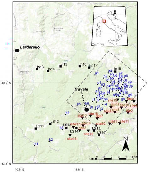
Figure 1.
The Larderello-Travale geothermal area. The 86 MT sites are located in the study area around Travale and were acquired during three different MT campaigns in 1992 (black-labeled sites), 2004 (blue-labeled sites), and 2006–07 (red-labeled sites). Only a subset of 51 sites belonging to the 2004 dataset were selected for 3D inversion because of their low level of noise, similarity of the period range, and the regular spatial distribution of the site locations. The dashed box represents the central area of the 3D model mesh.
Even though several differences occur, the Larderello and Travale fields belong to a common deep geothermal reservoir []. The Travale geothermal area is located to the south-east of the town of Larderello and covers a surface of around 50 km2 []. Here, in 2018, 38 wells and 8 plants were in production with an installed capacity of 200 MWe. Two main reservoirs comprise the Travale geothermal field [,,]. The shallow reservoir is a conventional hydrothermal system hosted in the evaporite-carbonate units with an average temperature of around 200 °C. The deep reservoir is hosted by the metamorphic basement and Neogene granitoids at a depth of about 2500–4000 m. The recent deep exploration program started in 1992, registering superheated steam at 350 °C with an initial pressure of 7 MPa at a depth of around 4 km [,]. Temperature logs from wells measured 300–350 °C at a depth of 3 km [,].
The Travale area is located in the inner part of the Northern Apennines, a sector of the Apennine orogenic belt that developed as a consequence of the Cenozoic collision between the European (Corso-Sardinian block) and the Adria plates []. The tectonic evolutional model of the Northern Apennines, proposed by several authors [,,], and references therein, implies two main deformational processes: (i) an initial one related to eastward-migrating compressional tectonics and (ii) a subsequent extensional tectonic process that migrated eastward, and which has been affecting the inner part of the orogenic belt since at least the early Miocene. Alternative models have also been proposed to describe the tectonic evolution of the inner Northern Apennines [,]. These models have revealed a complex tectonic evolution during the Miocene–Pleistocene with alternating compressive and extensional tectonic events, which contrast with the previously cited model supporting uninterrupted regional extensional tectonics since the early Miocene.
The geological framework of the Travale area is well documented [,,,]. Figure 2a reports a simplified geological map of the Travale geothermal area based on data from the Tuscany regional website (Geoportale Geoscopio website []). Figure 2b shows a NW-SE-oriented schematic structural model of the Travale area []. The outcropping carbonate formations represent the recharge area of the shallow reservoir, which is cooled down and is therefore less exploited than the deep reservoir. The structural-stratigraphic conceptual model is depicted in Figure 2c and outlines the following geological units: (1) Neogene sediments, (2) Ligurian and sub-Ligurian complex (Jurassic–Eocene), (3) Tuscan Nappe (Triassic–Lower Miocene), (4) tectonic wedge complex (Paleozoic–Triassic), (5) phyllitic and quartzitic complex, (6) mica–schist complex, (7) gneiss complex, (8) Pliocene granite and Quaternary granite. The shallow geothermal reservoir is hosted in units three and four, while the deep metamorphic reservoir is found in units five, six, seven, and eight. The intrusive complex represents the heat source of this long-lived geothermal system [].
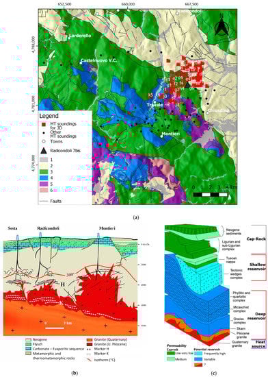
Figure 2.
(a) Simplified geological map of the area of study: (1) Quaternary deposits, (2) Neogene sediments (Miocene–Pliocene), (3) Ligurian and sub-Ligurian flysch complex (Jurassic–Eocene), (4) Tuscan Nappe sediments (Late Triassic–Early Miocene), (5) Tuscan Nappe: basal evaporites (Late Triassic), (6) Metamorphic units (Triassic–Paleozoic). The red squares are the 51 sites selected for MT inversion. Radicondoli7bis is the well shown in Figure 13. The black curves are the main faults []; (b) Schematic conceptual model of the Travale area with NW-SE orientation where seismic horizons H and K are indicated (modified from []); (c) Schematic sketch of the tectono-stratigraphic and hydrogeological complexes of the LTGA (modified from [,]).
From seismic reflection data, two seismic markers have been detected in the deep structure of the Travale field [,,]. The shallow marker is referred to as the “H-horizon” and appears as a discontinuous high-amplitude reflector. It is located in the metamorphic reservoir at a depth of 2.5–4 km, above the Pliocene granitoids, and represents the actual reservoir target (see Figure 2b). In fact, most of the drilled wells encountering the H-horizon are productive (e.g., in the sectors of Sesta, Radicondoli, and Montieri depicted in Figure 2b) []. The deep marker “K-horizon” is represented by a high-amplitude discontinuous reflector showing local bright spot features at a range of depths between 3 km (in Larderello) and 8 km (in Travale). Its origin and nature are still under debate [,,,,]. The K-horizon has often been associated to the 400–450 °C isotherm and the occurrence of supercritical fluids, but recent deep drilling in the proximity of Larderello measured a temperature above the K-horizon of about 510 °C []. The most recent seismic study in the Travale area was a local earthquake tomography analysis derived by travel-time inversion []. The 3D model of P-wave velocity (vp) highlighted a deep-rooted low-velocity body (vp = 5.7 km/s) below the Travale area, between the H- and K-horizons (see Figure 2b).
The Travale geothermal area is characterized by a low gravity anomaly of about 10–20 mGal []. This anomaly is spatially coherent with the highest heat flow of about 200 mW/m2 measured at the surface. Thermal numerical-modeling studies were performed in order to investigate the nature of the heat source of the reservoir as well as to predict the future evolution of the geothermal system [].
Previous MT studies of the Travale geothermal area resulted in 2D resistivity models [,]. The 2D inversion followed the algorithm of Rodi and Mackie [], using a priori geological sections of the profiles as their starting model. The inversion results showed, in essence, a highly conductive shallow subsurface and a large resistive body (around 800 Ω·m) overlying the K-horizon from a depth of 3 to 6 km. However, since previous studies are limited to 2D interpretation, this MT dataset needs to be re-examined in the light of the most recent 3D MT inversion techniques.
3. The MT Dataset
3.1. Acquisition and Processing
The Travale geothermal field was explored by means of three MT campaigns conducted in 1992, 2004, and 2006–07 [,]. The sites are depicted in Figure 1 with different colors according to the year of acquisition. The investigated area covers a surface of 48 km2. The average distance from the coastline is 60 km. The minimum distance between the sites is 191 m (sites d8–d9) and the average distance is 3.8 km. The minimum and the maximum elevations are 314 m (site c9) and 652 m (site k5) a.s.l., respectively.
The acquisition settings of the three datasets were slightly different. The 1992 dataset is composed of two long E-W profiles and was acquired as part of an exploration project using Phoenix V-5 systems [,]. A remote reference processing technique was applied using the remote site located on the Island of Capraia (Tuscan Archipelago).
Regarding the 2004 dataset, four-component (and five-component for some sites) data were collected using the Phoenix MTU system in the frame of the INTAS (EU) Project. At each site, the MT signal was recorded overnight for (at least) 12 h in the range of 0.003–993 s. Quality controls were carried out on time series, spectra, and transfer functions and a strong noise signature was observed for some sites, as reported by []. The source of the noise for short-period MT data was related to the local power plants and geothermal exploiting activities. To solve this, the remote-reference processing technique was applied using simultaneously measured data at the local sites. Long-period MT data were contaminated by noise arising from nearby electrified railways. To solve this, a remote site was placed in Sardinia, around 500 km southwest of Travale. The whole dataset was processed using the Phoenix Geophysics software [], based on the remote reference robust processing method [].
The 2006–07 dataset was acquired in the context of the I-GET (EU) Project. Long-period MT data (period range: 0.2–1000 s) were measured using the MT systems “NIMS” or “LEMI,” while audio-MT data (period range: 0.001–10 s) used a Stratagem system [].
In this study, the whole dataset depicted in Figure 1 (86 sites) was adopted for the dimensionality and directionality analyses. All the sites shown in Figure 1 are meant to provide a complete overview of the MT data previously acquired in Travale and to eventually foster new MT campaigns by ensuring high-quality data and regular site distribution on a 3D grid. The availability of a large MT dataset from different campaigns allowed for comprehensive dimensionality analysis. For 3D inversion modeling, we selected the subset of 51 MT soundings acquired in 2004. The main reasons for this choice were based on the low level of noise, the similarity of the period range covered by the responses and the regular spatial distribution of the site locations. Some MT sites were discarded from 3D inversion due to either their poor quality (the 2006–07 dataset) or to their inadequate spatial coverage (the 1992 dataset is composed of two isolated profiles around Larderello). These two factors would have corrupted the 3D modeling and the meshing, respectively.
The data quality of the sites selected for inversion is shown in Figure 3. The observed off-diagonal apparent resistivity is not corrected for static shift, which can explain some scattering of the curves.
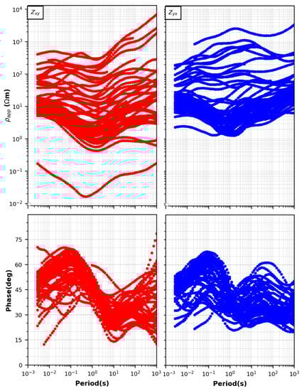
Figure 3.
Cloud plot of the observed off-diagonal apparent resistivity (top) and phase (bottom) at 51 sites selected for 3D inversion. The rotation of the impedance tensor is zero. xy-mode is plotted in red and yx-mode in blue without data errors. The phases are shifted in the first quadrant. The curves in the plot are raw data without any correction or rotation.
3.2. Dimensionality Analysis
The first evaluation of the raw dataset (before considering any static shift corrections or applying any rotation) involved a thorough analysis of the geoelectrical dimensionality by means of the rotational invariants of the impedance tensor [,], which gives an initial indication of the spatial distribution (1D, 2D, or 3D) of the electrical resistivity at depth and identifies the presence of galvanic distortion (3D/2D). Details are given in the Supplementary Material (Part A). The analysis results show a discrete number of 1D and 2D tensors for short periods and a predominant number of 3D cases, which clearly outlined the 3D nature of the subsurface electrical structures and thus the priority given to 3D inversion.
Further insight into the data came from the phase tensor analysis [,,]. The phase tensor (Φ) is based on the observed impedance tensor and returns a unique mathematical solution that, contrary to the invariants, is not affected by galvanic distortion []. Therefore, its analysis provides a distortion-free characterization of the strike and dimensionality as well as offering additional information for the interpretation of the underlying conductivity distribution.
The direction of the tensor and the three coordinate invariants (Φmin, Φmax, β) are graphically represented by means of the tensor ellipse, which discloses the orientation as well as the lateral variations of the underlying electrical structures. The phase tensor ellipses and their analysis for different periods are described in the Supplementary Material (Part A). The result confirms a general 3D dimensionality with scarce 1D and 2D cases at short periods. The strike direction was calculated for the whole period range from the impedance tensor Z (Figure 4a) [], the phase tensor azimuth (Figure 4b) [], and the induction arrows (Figure 4c). The three rose-diagrams of the strike direction are in good agreement and define the direction of N130°E for the geoelectrical strike. This strike direction was also estimated at each period decade (not reported here) and was consistent with that calculated considering all the periods. In detail, there was a clear strike direction in the range of 0.1–100 s because all the rose-diagram bins were aligned toward the preferred orientation of N130°E. At periods higher than 100 s, a leading direction of around N150°E was observed, but a small number of bins were oriented around N45°E.
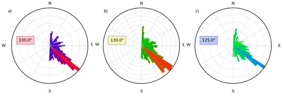
Figure 4.
Rose diagrams of the strike direction calculated over the whole period range from (a) the impedance tensor Z, (b) the phase tensor azimuth, and (c) the tipper vector. The color of the bars depends on the number of occurrences in each histogram bin and goes from purple to red for the invariants (a), from green to orange for the phase tensor (b), and from green to blue for the tipper (c).
The geomagnetic transfer function, also known as the tipper, represents the ratio between the vertical and horizontal components of the magnetic field. Figure 5 shows the tipper vectors (or induction arrows) of the subset of 26 sites (out of 51) whose vertical transfer function has been measured. The color scale of the ellipses ranges from 0° to 90° and refers to the phase-tensor determinant. It deviates from an angle of 45° if there is no 1D regional distribution in the subsurface. For the selected periods of 1 and 10 s (Figure 5a,b, respectively), the induction arrows present a substantial agreement with the strike direction shown in Figure 4 since they are orthogonal. We adopted the Parkinson criterion to represent the induction arrows, which point toward the region of highest conductance. The vectors suggest a possible NW-SE-oriented conductive region (in line with the phase-tensor ellipses shown in Supplementary Material, Part A).
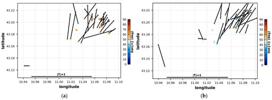
Figure 5.
Phase tensor and induction arrows at (a) 1 s and (b) 10 s for the 26 MT sites (Parkinson criterion). The horizontal arrow on the bottom shows the arrow length for a case of magnitude 1. The color scale refers to the determinant of the phase-tensor ellipse.
The outcome of the dimensionality analysis of the three complete datasets is interestingly related to the geology of the area. Firstly, the direction of the geoelectrical strike corresponds to the NW-SE-oriented major tectonic structures and surface geological units, as shown in the map of Figure 2a. This points out the role of the NNW-SSE-oriented Radicondoli sedimentary basin, which is located to the northeast of the study area (sensu [] or []). Secondly, the ellipses and the tippers at all periods seem to be sensitive to a possible large-scale deep structure oriented about N30–40°E along a certain strike that is transverse to the Apennines (see Supplementary Material, Part A).
The detailed analysis carried out in this section proves that, although a 2D strike direction of around N130°E could be considered as a “first order approximation,” as also suggested by the regional 2D trend of the surface geology, proper interpretation of our data requires 3D MT inversion.
3.3. Static Shift Correction by Means of TDEM Data
TDEM data have often been combined with MT data from geothermal areas even though their depth of investigation is usually much lower than that of the geothermal target (see for example []). The TDEM method is commonly adopted to correct the MT static shift because it provides independent information, which is not affected by telluric distortion (for a detailed description of the correction method see []). We carried out a TDEM survey to manage the static shift that could affect the MT apparent-resistivity (ρapp) curves.
We acquired new TDEM soundings in 2019 in order to constrain the MT soundings placed in different geological settings and to ensure a wide spatial coverage. The soundings corresponded to eight MT sites: a1, b2, b6, e1, g1, k1, k4, and k5 (see Figure 1 for their locations). TDEM data were acquired using the TEM-FAST 48 system by the AEMR company. The acquisition configuration was a coincident loop of 100 × 100 m or 75 × 75 m, depending on the accessibility of the site. The injected current was 3 A, the turn-off time was 7–8 μs and a total of 32–40 samples were acquired in the range of 4–4000 μs.
The TDEM data were adopted in order to directly correct the static shift of the correspondent MT site by means of 1D joint optimization and, if needed, to support the correction of the closest MT site only if it was placed on the same outcropping geological formation [,]. The static shift correction hence involved six TDEM-MT sites (k1 and k4 are not included in the 3D inversion), plus ten of the closest MT sites. A larger TDEM survey was not possible due to logistical issues.
To correct the static shift, TDEM and MT data were jointly inverted following the method of [], based on particle swarm optimization (PSO). This metaheuristic approach performs the simultaneous 1D optimization of TDEM and MT data for each MT polarization. The algorithm optimizes both the model parameters, i.e., the resistivity model, and an additional parameter accounting for the static shift. The off-diagonal components of the impedance tensor of the selected MT sites were corrected for static shift in order to perform a 3D inversion of the corrected off-diagonal components to be compared with the inversion of the uncorrected off-diagonal components (see Section 5).
As an example, a typical outcome of the static shift correction using PSO is plotted in Figure 6 for xy and yx modes of site a1. Figure 6a shows the MT observed xy and yx apparent resistivity (red and blue dots, respectively) and the calculated response (red and blue crosses, respectively). There is a satisfactory overlap between the MT corrected curves and the TDEM data (black dots) at short periods. In the example, the multiplicative factors calculated for static-shift correction were Sxy = 9 and Syx = 2. Figure 6b displays the good agreement between the observed and modeled phases. Figure 6c plots the diagonal components whose low magnitude is evident for the observed xx component (green dots) at long periods.
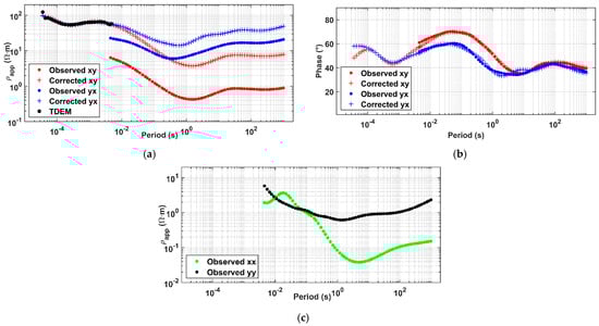
Figure 6.
Static shift correction for site a1 using PSO: (a) The dots are the observed apparent resistivity (ρapp) of TDEM (black) at short periods (up to 0.005 s) and of xy and yx MT (red and blue, respectively) from 0.003 s upward. The red and blue crosses indicate the predicted MT ρapp (xy and yx, respectively) that correct the static shift according to TDEM information; (b) Observed (dots) and predicted (crosses) xy and yx phases; (c) The diagonal apparent resistivity xx (green dots) and yy (black dots).
Regarding the other sites corrected for static shift, the majority of the original MT ρapp curves that, at the shortest periods, laid either above 100 Ω·m or below 10 Ω·m, were shifted within the range 10–100 Ω·m. In particular, the sites over the Neogene sediments (such as a1 and b2) had a corrected ρapp starting from around 100 Ω·m, while the sites on the Ligurian unit (such as e1 and d3) had a corrected ρapp starting from around 20–30 Ω·m. A detailed overview of the static-shift factors Sxy and Syx is depicted in Figure 7. The histograms show that the range of Sxy and Syx is 0.1–10 and most of them are lower than 2, thus meaning low correction factors. The grey bins in Figure 7 represent the ratio Sxy/Syx, which is generally lower than 1 and represents the level of correction between the two modes.
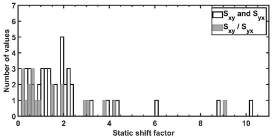
Figure 7.
Histograms of the static-shift factors Sxy and Syx (white bins) and their ratio Sxy/Syx (grey bins).
4. 3D MT Modeling and Inversion
The final dataset addressed by the inversion was composed of the 51 sites plotted as red squares on the geological map in Figure 2a. The complete period range was 0.003–1000 s, originally discretized into 75 values, then resampled into 20 values to unburden the time-consuming 3D computation. The resampling was calculated using a routine in the MTpy toolbox [].
The 3D inversion was performed using the ModEM software, which is available for the EM research community [,]. The inversion scheme of ModEM is based on the nonlinear conjugate gradient (NLCG) and the computation is parallelized. The objective function of the linearized inversion minimizes both the data misfit and model roughness, penalizing the deviations from the starting model. Inversion with different settings were executed using 96 cores (three nodes) of the high-performance computing (HPC) cluster of the Politecnico di Torino. The CPU model of the single node was an Intel Xeon Gold 6130 2.10 GHz with 21 TB (DDR4) of RAM. When the runs were computed, the sustained performance of the cluster was 21 TFLOPS. The computation time was around one hour per NLCG iteration.
The inversion settings, the 3D mesh, and the results were prepared and analyzed using the 3D-GRID Academic software. The domain was 130 km in the horizontal directions away from the model center and around 300 km deep, consistent with the boundary conditions and the electromagnetic skin depth. The mesh included the topography and bathymetry and the resistivity of the sea was fixed to 0.3 Ω·m. One important advantage of including the topography in the 3D model is that the forward computation compensates the static shift caused by topography [,,]. Along the horizontal directions, the model mesh was discretized into 100 × 100 cells, whose size was constant (140 m) for the central 70 × 70 cells, linearly increasing by a factor of 1.37 for the external cells (15 planes for each lateral side towards the boundary of the domain). The vertical direction was discretized into 65 layers, whose thickness was 28 m for the first layer, then increasing by a factor of 1.2.
We performed an extensive number of inversion tests in order to find the model (affected by equivalence) that has the best data fitting and agreement with the complex geology of the Travale geothermal field. The settings of the different inversion tests are summarized here, and fully explained in the Supplementary Material (Part B). These settings regard the starting model, smoothing factors, mesh orientation, tensor(s) to be inverted, and correction of the static shift for some sites. These settings were chosen following the most recent literature findings but also adapted to our specific dataset.
The starting model used for the inversion was a homogeneous half space of 100 Ω·m, which was selected after testing four different resistivity values (10, 100, 300, and 1000 Ω·m). Figure S3 in Supplementary Material shows that the lowest RMSE (1.05) was achieved with the fewest number of iterations by the inversion test using a 10-Ω·m homogeneous starting model. However, the 100-Ω·m resistivity value yielded the second lowest RMSE (1.15) and, since it was coherent with the average apparent resistivity of the sites after static shift correction, it was chosen for the starting model. We also performed a further inversion test with an a priori starting model derived from the 2D inversion result of []. It is provided in Supplementary Material (Part B).
The smoothing factor controls the model regularization along the three dimensions. Its choice was as critical as that of the starting model because of the over-parametrization of the inverse problem, which can lead to different outcomes []. After some trials, we set the smoothing factor to 0.2 for the horizontal directions and 0.1 for the vertical direction, in order to emphasize the vertical contrasts among the deep structures. When the inversion was initialized by the a priori starting model (test C in Supplementary Material, Part B), the smoothing factors were increased to 0.5 and 0.4, respectively, in order to test, on one hand, if the a priori resistivity contrast could be smoothed—despite the ModEM approach of minimal deviations from the starting model—and, on the other hand, if it was in fact required by the data.
The coordinate system was aligned with the geoelectrical strike. Even though the coherence between the strike direction and the rotation of the model mesh and data is fundamental in 2D modeling, it has turned out to be critical in 3D modeling as well [,,]. The authors of [] demonstrated that the 3D inversion result is dependent on the coordinate system and recommended a strike-oriented model mesh since it mostly minimizes the coupling among the four components of the impedance tensor (which, in ModEM, are handled independently). The MT data (Z and T) were rotated to N50°W (which is the same rotation as N130°E). The location of the MT sites was rotated to N50°E with respect to the mesh in order to simulate a mesh rotation of N50°W, because ModEM assumes that the data and the mesh are rotated in the same direction. We also performed two inversion tests (tests A and B in Supplementary Material, Part B) with the coordinate system aligned to the geographic north (N0°) and the MT data (Z and T) not rotated.
The uncorrected off-diagonal components of Z were inverted together with the tipper data. Even though in a 3D environment the information about the subsurface resistivity distribution is included in all the tensor elements, which can improve the spatial resolution, we neglected the inversion of the on-diagonal components since they had a relatively high magnitude. The inversion of the tipper T was included to improve the sensitivity at depth and to seek out lateral constraints []. After evaluating the quality of our data for the inversion, we selected 24 out of 26 sites with the tipper.
For the sake of completeness, the other inversion tests performed are supplied in Supplementary Material (Part B). They encompass the inversion of: uncorrected Z and T (tests A, C, D), uncorrected Z (test B), uncorrected off-diagonal components of Z with (test E) and without the tipper (test F), static-shift corrected off-diagonal components of Z (test G) considering the sites corrected for static shift (see Section 3.3).
The error floor was set as a portion of the absolute value of the impedance components (|Zij|) instead of as a portion of the mean of the off-diagonal components (|Zxy· Zxy|0.5), because the mean value could have underestimated one component of the tensor with respect to the other ones []. Since the original errors of the data were not negligible, the error associated with the data was set as the maximum between the original error and an error floor of 10% for the off-diagonal components of Z, and of 15% for the on-diagonal components of Z, which generally presented high magnitudes. The error floor of the tipper components was assigned by taking into account the error ratio between the impedance and the geomagnetic transfer function [], that is, equal to the error floor set for the impedance, i.e., 10% of the absolute value.
5. Inversion Result
The result we present in this section is the outcome of the inversion performed on the strike-aligned mesh starting with a 100 Ω·m homogeneous model and using the off-diagonal components of Z and T. The error floor was 10% for Zxy, Zyx, and the T. We consider this outcome to be the reference model among the other tests performed for two reasons: it is the most representative model of the geology of the area and it has the best data fitting for the off-diagonals at long periods (the calculated responses for selected sites are shown in Supplementary Material, Part C). In fact, the exclusion of the diagonals improved the data fitting with little effect on the model structures thanks to the inclusion of the tipper data. Furthermore, this inversion did not consider the static shift corrections, but given that we had rotated the data, and that only information from TDEM was available at some sites, it would have added doubts if this correction had been applied to the proper components of the tensor.
The inversion ended when the RMSE did not further decrease (and the minimum damping factor was reached). The total number of iterations was 71 and the final RMSE was 1.12.
The 3D resistivity model obtained is shown in Figure 8, Figure 9 and Figure 10. (The figures have not been smoothed, but represent the original cell-by-cell visualization.) Figure 8 shows the resistivity distribution in the horizontal plane at six different depths (27 m a.s.l., 222 m, 722 m, 1.4 km, 3.1 km, and 5.3 km b.s.l.) as they reveal the most evident resistivity contrasts of the imaged model. In the shallow structures (Figure 8a,b), we observe a clear difference between the northeastern conductive region roughly oriented NW-SE (<10 Ω·m), hereafter C1, and the southwestern region, hereafter R1, where the resistivity rises by up to 300 Ω·m. From 1 to 2.5 km b.s.l., the resistivity increases up to 180 Ω·m in a resistive body (R2 in Figure 8d). Below a depth of 3 km (Figure 8e,f), a resistive body of maximum 140 Ω·m, hereafter R3, elongates orthogonally to the strike (i.e., in parallel to the y-axis).
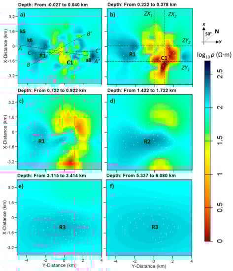
Figure 8.
Horizontal view of the 3D resistivity model for different depth slices: (a) 27 m a.s.l.; (b) 222 m b.s.l.; (c) 722 m b.s.l.; (d) 1.4 km b.s.l.; (e) 3.1 km b.s.l.; (f) 6 km b.s.l. This strike-oriented mesh has the north rotated 50° clockwise to be coherent with the data rotation of N50°W. The black-dashed profile AA′ drawn in (a) (from site k5 to a8) is the cross-section reported in Figure 9. Profiles BB′ and CC′ are shown in Figures 12 and 15, respectively. The dashed lines in (b) are the vertical cross-sections of Figure 10.
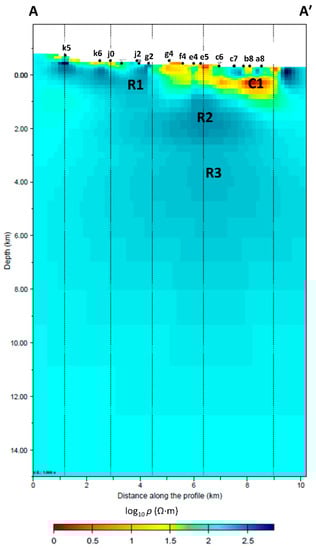
Figure 9.
Vertical cross-section of the model corresponding to the MT profile investigated by []. The SW-NE profile is orthogonal to the strike direction and crosses sites from k5 to a8 (see AA′ in Figure 8a). The vertical dotted lines are the traces of the multi-segment section.
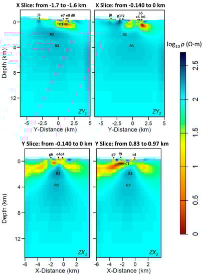
Figure 10.
Vertical cross-sections of the model: (top) ZY sections at X = −1.7 km (ZY1) and −0.14 km (ZY2); (bottom) ZX sections at Y = −0.14 km (ZX1) and 0.83 km (ZX2). The traces of these sections are plotted in Figure 8b.
The vertical cross-section depicted in Figure 9 is directly comparable with the 2D model of []. The most important feature between the depths of 3 and 8 km is a large 140-Ω·m body (R3). The R3 body extends orthogonally to the strike direction, as imaged also in the horizontal view of Figure 8e–f. Figure 10 shows the vertical cross-sections along the ZY and ZX planes (the traces of these sections are marked in Figure 8b).
The RMSE of 1.12 can be appreciated from Figure 11a,b, which plots the distribution of the RMSE in the frequency–space domain for Z and T, respectively. The final RMSE normalized for the full period bandwidth was 0.87 for Z and 1.5 for T. The lowest RMSE for Z was measured in site g1 (0.5) and for T in site b8 (0.6). The worst RMSE resulted in site e1 (1.4) for Z and in site c1 for T (3.4).
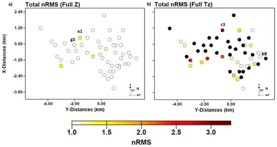
Figure 11.
Distribution of RMSE at each site. (a) Total normalized RMSE for the impedance tensor Z. (b) Total normalized RMSE for the tipper vector (T). The black dots in (b) mean no tipper data. The errors are normalized for the full period.
6. Discussion
We have explored different inversion setups in this study because 3D inversion in geothermal areas is potentially challenging, mainly due to the complex geology. The strike-aligned approach and the exclusion of the on-diagonals of Z had the advantage of improving the data fitting at long periods.
The xy-plane view of the resistivity distribution at shallow depth in Figure 8a is in agreement with the expected resistivity of the outcropping rocks described in the geological map reported in Figure 2a. The northeastern conductive area (C1) mostly corresponds to the Neogene sediments and the Ligurian complex, and was imaged up to a depth of around 1200 m b.s.l. (see Figure 8a and Figure 9). The central mildly resistive area (10–50 Ω·m) between C1 and R1 in the horizontal view of Figure 8b corresponds to the spatial coverage of the Ligurian and sub-Ligurian flysch complex. Finally, the southern region R1, showing resistivities up to 300 Ω·m, matches the sediments and carbonates of the Tuscan nappe. It should be noted, however, that the irregular space-covering of the sites may have influenced the shape of the imaged resistive structures, as can be seen in Figure 8. Figure 8e,f displays the loss of resolution with depth, which can be explained by two main reasons. The first reason is related to the dataset, because the spatial aperture of the MT survey, which should be twice the intended depth of investigation, prevented a deep geometrical constraint of the 3D structures []. The second reason regards the imaged shallow conductors, such as C1, which reduced the maximum skin depth calculated from the impedance determinant to a few tens of kilometers (instead of several hundreds of kilometers for the sites far from C1).
Interestingly, we found a resistivity contrast in correspondence with the bottom of the Ligurian units (and Neogene sediments) of the Radicondoli basin, separating them from the underlying units piled in the chain (from []). Figure 12 shows a north–south section of the model crossing sites from a4 to j3. The geological surface (black-dashed line) was processed in Petrel software from the findings of [] and represents the base of the cap-rock (Neogene and Ligurian units). To the north (below site b4) the basin-bottom surface descends from a depth of around 600 to 1500 m b.s.l., where the resistivity jumps from 4 Ω·m to 40 Ω·m. This represents a remarkable agreement between a 3D resistivity contrast and a geological surface from the known geological model.
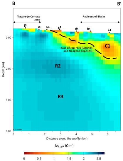
Figure 12.
The vertical cross-section of the 3D resistivity model is compared to the black-dashed line corresponding to the base of the geological unit of Neogene and Ligurian units (from []). The north–south section crosses sites from j3 to a4 (see profile BB′ in Figure 8a). The coordinates of the section edges are (latitude north-longitude east): 43.1688°–11.0115° (left) and 43.2051°–11.0736° (right).
The vertical section of the 3D model in Figure 9 crosses the sites belonging to the 2D profile investigated by []. The resistivity distribution of the 3D model is partially similar to that of the 2D model, but some features emerged from the 3D inversion. The shallow structure R1 (up to 1 km b.s.l.) beneath sites k5–j2 is far more resistive (300 Ω·m) than in the 2D model. Beneath sites g4–a8, from 1 to around 3 km b.s.l., the 3D model has a resistive region R2 (180 Ω·m) rather than a conductive anomaly as seen in the 2D model. The resistive body R3 at 3–8 km b.s.l. has a different shape, boundaries, and resistivity values compared to the 2D model. Given all these dissimilarities, our result overcame the main limitations of the 2D model, which could have been strongly biased by its chosen a priori geological cross-section starting model. Moreover, the 2D model might have missed some heterogeneities due to the adoption of a 2D approach for the inversion of 3D data.
The volume R2, with more than 180 Ω·m at a depth of about 1–2.5 km, is embedded between the low-resistive cap-rock (C1) and the 140 Ω·m R3 body. The interpretation of R2 is challenging due to the interplay of multiple processes. At this depth, heterogeneous units (tectonic wedge complex (TWC) and phyllites) mostly occur across a very wide range of electrical resistivities (from 10−1 Ω·m to 104 Ω·m) measured in the geophysical well logs, such as the wells Radicondoli 7bis and Montieri 4 in the area of interest []. Figure 13 shows a comparison between the well log resistivity along the Radicondoli 7bis and the correspondent 1D resistivity profile extracted from our 3D MT model. At the depth of the TWC and metamorphic units (below about 750 m), an averaged MT response is obtained considering the higher order of magnitude of the investigated volume with respect to the resistivity log that recorded a huge variability of the resistivity. At shallow depths (above 750 m), the resistivity from the model was higher than that from the log. In this case, the shallow cap-rock is not properly imaged, probably because the well is located at the boundary of the area covered by the MT sites (see Figure 2a). There, the model resistivity keeps the starting value of 100 Ω·m, while where the model is better constrained, the cap-rock is properly imaged with a lower resistivity. Even though highly resistive volumes were measured in the heterogeneous units (TWC and phyllites), the embedded extremely low resistivity values (probably owing to graphite) have affected the measured EM signal, which provided an averaged resistivity of this geological unit. This phenomenon is known to occur in the Larderello geothermal system following a case where research was conducted in another sector of the field in the proximity of Lago Boracifero by means of EM measurements and an experimental Surface-Hole Deep ERT [,,]. In the central part of the study area, the 3D model is characterized by a well-defined volume of increased resistivity (R2), which elongates transversely to the Apennines (see Figure 8e,f and Figure 13). A factor that can play a role in the increased resistivity is the occurrence of the vapor-dominated hydrothermal circulation. Indeed, part of the exploited reservoir is located at the same depth as R2. We point out the match between R2 and the current geothermal target represented by the seismic H-horizon along the seismic profile from [] (see Figure 15). It is possible that in other sectors of the investigated area the H-horizon can lie in correspondence with R3. Further investigations with complete seismic datasets would be beneficial.
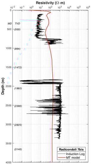
Figure 13.
Well log resistivity (induction log M2R6) from the Radicondoli 7bis well (black line) and resistivity extracted from the 3D model (red line). On the vertical axis, MD is the measured depth and TVD is the true vertical depth. The location of the well is shown in Figure 2a.
The deep resistive body R3 (see Figure 8e–f, Figure 9 and Figure 10) was imaged in all the inversion tests and showed high resistivities (>140 Ω·m) between the depths of 3 and 8 km. Figure 14 displays the 3D model with a cutaway view on the 160 Ω·m isosurface. Further inspection of the 3D model is supplied in Supplementary Material with a brief animation. For the first time the deep resistive body of the Travale geothermal field, already known from 2D inversion, is revealed with its position and orientation in three dimensions. From Figure 14, the R3 body is oriented orthogonally to the main Apennine strike direction. This was expected because some of the soundings showed a strike direction of N40–50°E at long periods (see Supplementary Material, Part A). The orientation of R2 and R3 represents a major improvement in the knowledge of the Travale geothermal field. A strict relation between the strike-slip tectonics transversal to the Apennine direction and fluid circulation was recently claimed by various studies [,,,].
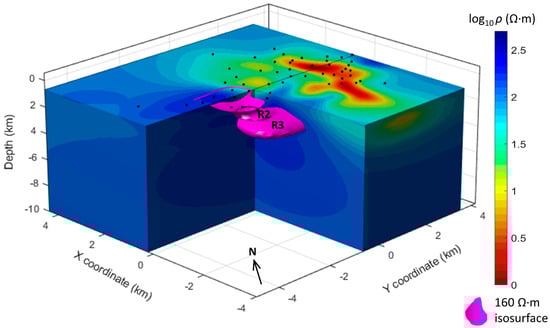
Figure 14.
The 3D model displayed with a cutaway view on the 160 Ω∙m isosurface. The deep resistive bodies R2 and R3 are directed about N40°E. The black dots represent the MT sites.
To assess if R3 was necessary to fit the data, we carried out a sensitivity analysis (see Supplementary Material, Part C, for details). R3 was replaced with a perturbed body of 1, 20, 50, and 100 Ω·m in four different sensitivity tests, respectively. The 1 Ω·m perturbed model most significantly worsened the RMSE. The recalculation of the forward problem led to an overall RMSE increase of 75% and to an RMSE increase from 57% to 101% for the sites directly above the body (see Figure S17 in the Supplementary Material for a representative site). The sensitivity analysis proved that the model is most sensitive to the lowest resistivity value of the perturbed body (1 Ω·m) and that the data are incompatible with a resistivity lower than 50–100 Ω·m for R3, given the limitations of the poor resolution at this depth.
In order to interpret the resistive body R3 below the Travale field, we compared the 3D resistivity model with the 3D local earthquake tomography by []. An analogy occurs between the resistive body R3 and the low-velocity body detected in the vp images below the Travale area along an available profile (see Figure 15 from profile CC′ plotted in Figure 8a). The velocity model reported a 5-km-wide low-velocity body (vp about 5 km/s) that was deeply rooted in the crust. Furthermore, that authors showed the occurrence of a large number of hypocenters inside and surrounding the low-velocity volume (5–5.5 km/s), which is highly comparable in shape to R3. This implies the occurrence of a fragile regime and rock fracturing. It is worth noting from [] that the largest hypocenter cluster corresponds to a high-velocity anomaly below the K-horizon, a region which is unfortunately not covered by our MT survey. It should be noted that, in [], the trend of the low-velocity body is different from that of our R3 body, but some tests performed in [] also showed a transverse NE-SW trend in the area.
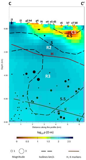
Figure 15.
A vertical cross-section drawn from the 3D resistivity model is compared with the 3D seismic velocity model from local earthquake tomography by []. The R3 body (>140 Ω·m) and the low-velocity body with vp around 5–5.5 km/s both extend between the depths of 3 and 8 km. The trace of the cross-section is the profile CC′ in Figure 8a and it corresponds to the seismic profile CC′ of Figure 6 in []. The dashed lines represent the absolute seismic P-wave velocity (from 4.5 to 6 km/s). The red contour lines are the isodepths of the H- and K-horizons (from [] and references therein). The black circles represent the hypocenters and are proportional to the magnitude. The coordinates of the section edges are (latitude north-longitude east): 43.1667°–11.0240° (left) and 43.2124°–11.0732° (right).
Our interpretation of R3 is that it may be due to the effect of the interplay of a highly fractured volume of crystalline rocks hosting a high-temperature hydrothermal circulation and to the occurrence of a very large (crystallized) granitic intrusion, locally cored by some wells at depths between about 2–4.5 km. The resistive nature of the deep body is explained by the vapor-dominated condition of the reservoir, so that highly resistive fluids (vapors) circulate in highly resistive rocks (e.g., granites). Moreover, a pervasive mineral alteration, which would decrease the bulk resistivity of the rocks, has been excluded by well-cuttings and core-analyses carried out in this area as part of the I-GET project [,].
Our 3D model had limited resolution below R3, but showed an interesting relationship with the seismic marker K-horizon. The bottom of R3 is around 8 km deep (see Figure 9, Figure 10 and Figure 15) and could be reasonably associated with the depth of the K-horizon in this area (following []). We did not recognize the occurrence of melt fractions in the area of study down to 8 km. The occurrence of melted igneous intrusions cannot be excluded at a level deeper than 8 km or in the Travale area, which is not covered by our MT sites.
7. Conclusions
This work presents the first 3D resistivity model of the geothermal area of Travale (Italy) resulting from derivative-based 3D MT inversion.
The MT dataset was accurately analyzed in terms of geoelectrical dimensionality, strike direction, and phase tensor properties.
Given the equivalence of the solutions of the 3D MT inverse problem, we performed an extensive number of inversion tests by varying the initial parameters. These regarded the starting model, the data to be inverted, the grid rotation, and the correction of the static shift for some selected sites. The static shift was corrected for the off-diagonal components of the impedance tensor by means of TDEM soundings for those MT sites in correspondence with (or in the vicinity of) the TDEM acquisitions. After many tests, we have demonstrated that—if static-shift corrected data of the selected sites are included in the 3D modeling—the shallow structures are more homogeneous and the long period data fit better than for the test with uncorrected data (see Supplementary Material), but there was no appreciable improvement in the final RMSE and model. For these reasons, the 3D model for the final interpretation was selected from the inversion of uncorrected off-diagonal components and the tipper, using a strike-aligned mesh. This model has the best data fitting and agreement with the complex geology of the Travale geothermal system.
The selected model represents an important contribution to the investigation of the Travale geothermal field. The most important outcome is that the final model identifies and characterizes the region’s 3D subsurface structures. In this way, our results have expanded the knowledge of the subsurface by adding another spatial dimension, where until now it had only been estimated by means of 2D MT inversion. The validity of our results is supported by geological information, resistivity well logs, and seismic data:
- -
- A distinct correlation emerged between the resistivity contrast at shallow depths and the geological surface of the base of the Neogene sedimentary basin;
- -
- Two deep resistive bodies were imaged at depths of 1–3 km (R2) and 3–8 km (R3) with resistivities higher than 180 Ω·m and 140 Ω·m, respectively, with a N40–50°E orientation;
- -
- The mildly resistive body R2 lies in a region where the geophysical well logs measured a heterogeneous resistivity value (10−1 Ω·m–104 Ω·m);
- -
- A marked analogy was identified between the deep resistive body R3 and a low-velocity body (vp about 5 km/s) deeply rooted in the crust below the Travale area;
- -
- The role played by the vapor-dominated circulation is recognized in these high-resistivity bodies (R2 and R3), together with the occurrence of (crystallized) granitic intrusions contributing to R3.
Three-dimensional MT inversion was challenging due also to the time-consuming computation which can require 100 times more unknowns than a 2D inversion. Furthermore, the geology of the area is extremely complex and the framework of the geothermal system is still under debate. Our work offers the first interpretation of the 3D subsurface electrical distribution in the Travale area from a geophysical perspective and could pave the way to further insight about the geothermal system.
Future work should broaden the MT characterization of the Travale area by means of new acquisition campaigns that would enlarge the investigated zone, ideally with a regularly spaced coverage of the sites, and would moreover improve the data quality according to the most recent acquisition techniques. The existing dataset needs to be expanded to all the sites with the acquisition of the geomagnetic transfer function, which may significantly improve the outcome of the 3D inversion. Joint inversion or the integration of multiple geophysical datasets (e.g., gravity, surface waves, electric) would also be beneficial to a comprehensive study of the geothermal system.
Supplementary Materials
The following are available online at https://www.mdpi.com/article/10.3390/rs14030542/s1. Part A: Details on the dimensionality analysis and starting model. Figure S1: Dimensionality analysis; Figure S2: Phase tensor analysis; Figure S3: Choice of the starting model. Part B: The inversion tests performed on the MT data set of Travale. Table S1: Settings and RMSE values of the inversion tests; Figures S4–S15: Results from the 3D MT inversion tests and their RMSE distribution. Part C: Model responses and sensitivity tests. Figures S16 and S17: Sensitivity analysis on the deep resistive body R3. Video S1: animation of the 3D model.
Author Contributions
F.P.: data analysis and processing, investigation, methodology, data curation, software, writing—original draft preparation, writing—review and editing, visualization; A.M. (Anna Martí): methodology, data curation, software, validation, writing—review and editing, supervision, conceptualization; P.Q.: methodology, validation, writing—review and editing, supervision; A.S.: investigation, data curation, validation, writing—review and editing; A.M. (Adele Manzella): validation, writing—review and editing, supervision; J.L.: methodology, software, validation, writing—review and editing, supervision; A.G.: investigation, validation, writing—review and editing, supervision. All authors have read and agreed to the published version of the manuscript.
Funding
This research received no external funding.
Institutional Review Board Statement
Not applicable.
Informed Consent Statement
Not applicable.
Data Availability Statement
Not applicable.
Acknowledgments
Gary Egbert, Anna Kelbert, and Naser Meqbel are thanked for providing the ModEM code. Naser Meqbel (Consulting-GEO) kindly provided the 3DGRID software for research purposes. Computational resources provided by hpc@polito (http://hpc.polito.it). The Magnetotelluric data were acquired in the frame of the European INTAS grant (03-51-3327), I-GET Project (FP6, G.A. 518378), exploration projects and kindly provided by CNR, National Research Council of Italy. We acknowledge Enel Green Power for sharing some of the data used for the dimensionality analysis.
Conflicts of Interest
The authors declare no conflict of interest.
References
- Pellerin, L.; Johnston, J.M.; Hohmann, G.W. A numerical evaluation of electromagnetic methods in geothermal exploration. Geophysics 1996, 61, 121–130. [Google Scholar] [CrossRef]
- Spichak, V.; Manzella, A. Electromagnetic sounding of geothermal zones. J. Appl. Geophys. 2009, 68, 459–478. [Google Scholar] [CrossRef]
- Muñoz, G. Exploring for geothermal resources with electromagnetic methods. Surv. Geophys. 2014, 35, 101–122. [Google Scholar] [CrossRef]
- Mitjanas, G.; Ledo, J.; Macau, A.; Alías, G.; Queralt, P.; Bellmunt, F.; Rivero, L.; Gabàs, A.; Marcuello, A.; Benjumea, B.; et al. Integrated seismic ambient noise, magnetotellurics and gravity data for the 2D interpretation of the vallès basin structure in the geothermal system of la garriga-samalús (NE Spain). Geothermics 2021, 93, 102067. [Google Scholar] [CrossRef]
- Mackie, R.L.; Madden, T.R. Three-dimensional magnetotelluric inversion using conjugate gradients. Geophys. J. Int. 1993, 115, 215–229. [Google Scholar] [CrossRef] [Green Version]
- Newman, G.A.; Alumbaugh, D.L. Three-dimensional magnetotelluric inversion using non-linear conjugate gradients. Geophys. J. Int. 2000, 140, 410–424. [Google Scholar] [CrossRef] [Green Version]
- Avdeev, D.; Avdeeva, A. 3D magnetotelluric inversion using a limited-memory quasi-newton optimization. Geophysics 2009, 74, F45–F57. [Google Scholar] [CrossRef] [Green Version]
- Siripunvaraporn, W.; Egbert, G. WSINV3DMT: Vertical magnetic field transfer function inversion and parallel implementation. Phys. Earth Planet. Inter. 2009, 173, 317–329. [Google Scholar] [CrossRef]
- Egbert, G.D.; Kelbert, A. Computational recipes for electromagnetic inverse problems: Computational recipes for EM inverse problems. Geophys. J. Int. 2012, 189, 251–267. [Google Scholar] [CrossRef] [Green Version]
- Čuma, M.; Gribenko, A.; Zhdanov, M.S. Inversion of magnetotelluric data using integral equation approach with variable sensitivity domain: Application to earthscope MT data. Phys. Earth Planet. Inter. 2017, 270, 113–127. [Google Scholar] [CrossRef]
- Singh, A.; Dehiya, R.; Gupta, P.K.; Israil, M. A MATLAB based 3D modeling and inversion code for MT data. Comput. Geosci. 2017, 104, 1–11. [Google Scholar] [CrossRef]
- Grayver, A.V. Parallel three-dimensional magnetotelluric inversion using adaptive finite-element method. Part I: Theory and synthetic study. Geophys. J. Int. 2015, 202, 584–603. [Google Scholar] [CrossRef] [Green Version]
- Kordy, M.; Wannamaker, P.; Maris, V.; Cherkaev, E.; Hill, G. 3-D magnetotelluric inversion including topography using deformed hexahedral edge finite elements and direct solvers parallelized on SMP computers—Part I: Forward problem and parameter jacobians. Geophys. J. Int. 2016, 204, 74–93. [Google Scholar] [CrossRef]
- Kruglyakov, M.; Kuvshinov, A. 3-D inversion of MT impedances and inter-site tensors, individually and jointly. New lessons learnt. Earth Planets Space 2019, 71, 4. [Google Scholar] [CrossRef] [Green Version]
- Kelbert, A.; Meqbel, N.; Egbert, G.D.; Tandon, K. ModEM: A modular system for inversion of electromagnetic geophysical data. Comput. Geosci. 2014, 66, 40–53. [Google Scholar] [CrossRef]
- Spichak, V.; Popova, I. Artificial neural network inversion of magnetotelluric data in terms of three-dimensional earth macroparameters. Geophys. J. Int. 2000, 142, 15–26. [Google Scholar] [CrossRef]
- Xiang, E.; Guo, R.; Dosso, S.E.; Liu, J.; Dong, H.; Ren, Z. Efficient hierarchical trans-dimensional bayesian inversion of magnetotelluric data. Geophys. J. Int. 2018, 213, 1751–1767. [Google Scholar] [CrossRef]
- Conway, D.; Simpson, J.; Didana, Y.; Rugari, J.; Heinson, G. Probabilistic magnetotelluric inversion with adaptive regularisation using the No-U-Turns sampler. Pure Appl. Geophys. 2018, 175, 2881–2894. [Google Scholar] [CrossRef]
- Pace, F.; Santilano, A.; Godio, A. A review of geophysical modeling based on particle swarm optimization. Surv. Geophys. 2021, 42, 505–549. [Google Scholar] [CrossRef]
- Uchida, T.; Sasaki, Y. Stable 3D inversion of MT data and its application to geothermal exploration. Explor. Geophys. 2006, 37, 223–230. [Google Scholar] [CrossRef]
- Piña-Varas, P.; Ledo, J.; Queralt, P.; Marcuello, A.; Bellmunt, F.; Hidalgo, R.; Messeiller, M. 3-D magnetotelluric exploration of tenerife geothermal system (Canary Islands, Spain). Surv. Geophys. 2014, 35, 1045–1064. [Google Scholar] [CrossRef]
- Lindsey, N.J.; Newman, G.A. Improved workflow for 3D inverse modeling of magnetotelluric data: Examples from five geothermal systems. Geothermics 2015, 53, 527–532. [Google Scholar] [CrossRef] [Green Version]
- Di Paolo, F.; Ledo, J.; Ślęzak, K.; Martínez van Dorth, D.; Cabrera-Pérez, I.; Pérez, N.M. La Palma Island (Spain) geothermal system revealed by 3D magnetotelluric data inversion. Sci. Rep. 2020, 10, 18181. [Google Scholar] [CrossRef] [PubMed]
- Arias, A.; Dini, I.; Casini, M.; Fiordelisi, A.; Perticone, I.; Pisano, A. Geoscientific feature update of the larderello-travale geothermal system (Italy) for a regional numerical modeling. In Proceedings of the World Geothermal Congress, Bali, Indonesia, 25–29 April 2010; pp. 1–11. [Google Scholar]
- Moeck, I.S. Catalog of geothermal play types based on geologic controls. Renew. Sustain. Energy Rev. 2014, 37, 867–882. [Google Scholar] [CrossRef] [Green Version]
- Santilano, A.; Manzella, A.; Gianelli, G.; Donato, A.; Gola, G.; Nardini, I.; Trumpy, E.; Botteghi, S. Convective, intrusive geothermal plays: What about tectonics? Geoth. Energ. Sci. 2015, 3, 51–59. [Google Scholar] [CrossRef]
- Gianelli, G. (Ed.) Geothermal Energy Research Trends; Nova Science Publishers: New York, NY, USA, 2008; ISBN 978-1-60021-683-1. [Google Scholar]
- Manzella, A. Resistivity and heterogeneity of earth crust in an active tectonic region, southern tuscany (Italy). Ann. Geophys. 2004, 47, 107–118. [Google Scholar] [CrossRef]
- Manzella, A.; Spichak, V.; Pushkarev, P.; Sileva, D.; Oskooi, B.; Ruggieri, G.; Sizov, Y. Deep fluid circulation in the travale geothermal area and its relation with tectonic structure investigated by a magnetotelluric survey. In Proceedings of the Thirty-First Workshop on Geothermal Reservoir Engineering, Stanford, CA, USA, 30 January–1 February 2006; pp. 1–6. [Google Scholar]
- Duprat, A.; Gole, F. Magnetotelluric soundings in the travale area, Tuscany. Geothermics 1985, 14, 689–696. [Google Scholar] [CrossRef]
- Hutton, V.R.S. Magnetic, telluric and magnetotelluric measurements at the travale test site, Tuscany, 1980–1983: An overview. Geothermics 1985, 14, 637–644. [Google Scholar] [CrossRef]
- Schwarz, G.; Haak, V.; Rath, V. Electrical conductivity studies in the travale geothermal field, Italy. Geothermics 1985, 14, 653–661. [Google Scholar] [CrossRef]
- Casini, M.; Ciuffi, S.; Fiordelisi, A.; Mazzotti, A.; Stucchi, E. Results of a 3D seismic survey at the travale (Italy) test site. Geothermics 2010, 39, 4–12. [Google Scholar] [CrossRef]
- Orlando, L. Interpretation of tuscan gravity data. Boll. Soc. Geol. Ital. 2005, 3, 179–186. [Google Scholar]
- Capozzoli, L.; De Martino, G.; Giampaolo, V.; Godio, A.; Manzella, A.; Perciante, F.; Rizzo, E.; Santilano, A. Deep Electrical Resistivity Model of the Larderello Geothermal Field (Italy): Preliminary Results of the FP7 IMAGE Experiment. In Proceedings of the 35° Convegno Nazionale Gruppo Nazionale di Geofisica della Terra Solida, Lecce, Italy, 22–24 November 2016; pp. 499–501. [Google Scholar]
- Gola, G.; Bertini, G.; Bonini, M.; Botteghi, S.; Brogi, A.; De Franco, R.; Dini, A.; Donato, A.; Gianelli, G.; Liotta, D.; et al. Data integration and conceptual modelling of the larderello geothermal area, Italy. Energy Procedia 2017, 125, 300–309. [Google Scholar] [CrossRef]
- Fiordelisi, A.; Moffatt, J.; Ogliani, F.; Caini, F.; Ciuffi, S.; Romi, A. Revised processing and interpretation of reflection seismic data in the travale geothermal area (Italy). In Proceedings of the World Geothermal Congress, Antalya, Turkey, 24–29 April 2005; pp. 1–10. [Google Scholar]
- De Matteis, R.; Vanorio, T.; Zollo, A.; Ciuffi, S.; Fiordelisi, A.; Spinelli, E. Three-dimensional tomography and rock properties of the larderello-travale geothermal area, Italy. Phys. Earth Planet. Inter. 2008, 168, 37–48. [Google Scholar] [CrossRef] [Green Version]
- Bagagli, M.; Kissling, E.; Piccinini, D.; Saccorotti, G. Local earthquake tomography of the larderello-travale geothermal field. Geothermics 2020, 83, 101731. [Google Scholar] [CrossRef]
- Manzella, A.; Ungarelli, C.; Ruggieri, G.; Giolito, C.; Fiordelisi, A. Electrical resistivity at the travale geothermal field (Italy). In Proceedings of the World Geothermal Congress, Bali, Indonesia, 25–29 April 2010; pp. 1–8. [Google Scholar]
- Siripunvaraporn, W. Three-dimensional magnetotelluric inversion: An introductory guide for developers and users. Surv. Geophys. 2012, 33, 5–27. [Google Scholar] [CrossRef]
- Bertani, R.; Bertini, G.; Cappetti, G.; Fiordelisi, A. An update of the larderello-travale/radicondoli deep geothermal system. In Proceedings of the World Geothermal Congress, Antalya, Turkey, 24–29 April 2005; pp. 1–6. [Google Scholar]
- Manzella, A.; Serra, D.; Cesari, G.; Bargiavchi, E.; Cei, M.; Cerutti, P.; Conti, P.; Giudetti, G.; Lupi, M.; Vaccaro, M. Geothermal energy use, country update for Italy. In Proceedings of the European Geothermal Congress, Den Haag, The Netherlands, 11–14 June 2019; pp. 1–19. [Google Scholar]
- Final Report on Integrated Application in Field Models (Magmatic Settings); IMAGE Final Report; IMAGE Project; EU FP7 Program; 2017; p. 266.
- Bertani, R.; Büsing, H.; Buske, S.; Dini, A.; Hjelstuen, M.; Luchini, M.; Manzella, A.; Nybo, R.; Rabbel, W.; Serniotti, L. The first results of the Descramble project. In Proceedings of the Forty-Third Workshop on Geothermal Reservoir Engineering, Stanford, CA, USA, 12–14 February 2018; pp. 1–16. [Google Scholar]
- Bertini, G.; Casini, M.; Ciulli, B.; Ciuffi, S.; Fiordelisi, A. Data revision and upgrading of the structural model of the travale geothermal field (Italy). In Proceedings of the World Geothermal Congress, Antalya, Turkey, 24–29 April 2005; pp. 1–8. [Google Scholar]
- Romagnoli, P.; Arias, A.; Barelli, A.; Cei, M.; Casini, M. An updated numerical model of the larderello–travale geothermal system, Italy. Geothermics 2010, 39, 292–313. [Google Scholar] [CrossRef]
- Barelli, A.; Cei, M.; Lovari, F.; Romagnoli, P. Numerical modeling for the larderello-travale geothermal system (Italy). In Proceedings of the World Geothermal Congress, Bali, Indonesia, 25–29 April 2010; pp. 1–9. [Google Scholar]
- Boccaletti, M.; Corti, G.; Martelli, L. Recent and active tectonics of the external zone of the northern apennines (Italy). Int. J. Earth Sci. 2011, 100, 1331–1348. [Google Scholar] [CrossRef]
- Carmignani, L.; Decandia, F.A.; Fantozzi, P.L.; Lazzarotto, A.; Liotta, D.; Meccheri, M. Tertiary extensional tectonics in tuscany (Northern Apennines, Italy). Tectonophysics 1994, 238, 295–315. [Google Scholar] [CrossRef]
- Jolivet, L.; Faccenna, C.; Goffé, B.; Mattei, M.; Rossetti, F.; Brunet, C.; Storti, F.; Funiciello, R.; Cadet, J.P.; d’Agostino, N.; et al. Midcrustal shear zones in postorogenic extension: Example from the Northern Tyrrhenian Sea. J. Geophys. Res. 1998, 103, 12123–12160. [Google Scholar] [CrossRef]
- Brogi, A. Neogene extension in the northern apennines (Italy): Insights from the Southern Part of the Mt. Amiata Geothermal Area. Geodin. Acta 2006, 19, 33–50. [Google Scholar] [CrossRef]
- Bonini, M.; Sani, F. Extension and compression in the northern apennines (Italy) hinterland: Evidence from the late miocene-pliocene siena-radicofani basin and relations with basement structures: Extension and compression in the apennines. Tectonics 2002, 21, 1-1–1-32. [Google Scholar] [CrossRef] [Green Version]
- Bellani, S.; Brogi, A.; Lazzarotto, A.; Liotta, D.; Ranalli, G. Heat flow, deep temperatures and extensional structures in the larderello geothermal field (Italy): Constraints on geothermal fluid flow. J. Volcanol. Geotherm. Res. 2004, 132, 15–29. [Google Scholar] [CrossRef]
- Bertini, G.; Casini, M.; Gianelli, G.; Pandeli, E. Geological structure of a long-living geothermal system, Larderello, Italy. Terra Nova 2006, 18, 163–169. [Google Scholar] [CrossRef]
- Geoportale Geoscopio. Available online: http://www502.regione.toscana.it/geoscopio/cartoteca.html (accessed on 1 July 2019).
- de Franco, R.; Petracchini, L.; Scrocca, D.; Caielli, G.; Montegrossi, G.; Santilano, A.; Manzella, A. Synthetic seismic reflection modelling in a supercritical geothermal system: An image of the k-horizon in the larderello field (Italy). Geofluids 2019, 2019, 8492453. [Google Scholar] [CrossRef]
- Vanorio, T.; De Matteis, R.; Zollo, A.; Batini, F.; Fiordelisi, A.; Ciulli, B. The deep structure of the larderello-travale geothermal field from 3D microearthquake traveltime tomography: P-velocity structure beneath larderello-travale. Geophys. Res. Lett. 2004, 31. [Google Scholar] [CrossRef] [Green Version]
- Sani, F.; Bonini, M.; Montanari, D.; Moratti, G.; Corti, G.; Ventisette, C.D. The structural evolution of the radicondoli–volterra basin (Southern Tuscany, Italy): Relationships with magmatism and geothermal implications. Geothermics 2016, 59, 38–55. [Google Scholar] [CrossRef]
- Rodi, W.; Mackie, R.L. Nonlinear conjugate gradients algorithm for 2-D magnetotelluric inversion. Geophysics 2001, 66, 174–187. [Google Scholar] [CrossRef]
- Fiordelisi, A.; Mackie, R.; Manzella, A.; Watts, D.; Zaja, A. Electrical features of deep structures of southern tuscany (Italy). Ann. Geophys. 1998, 41, 17. [Google Scholar] [CrossRef]
- Phoenix Geophysics Data Processing User Guide. 2005. Available online: http://www.phoenix-geophysics.com/Support/user_guides/guides/data-proc-v.3-online.pdf (accessed on 1 December 2020).
- Gamble, T.D.; Goubau, W.M.; Clarke, J. Magnetotellurics with a remote magnetic reference. Geophysics 1979, 44, 53–68. [Google Scholar] [CrossRef] [Green Version]
- Martí, A.; Queralt, P.; Ledo, J. WALDIM: A code for the dimensionality analysis of magnetotelluric data using the rotational invariants of the magnetotelluric tensor. Comput. Geosci. 2009, 35, 2295–2303. [Google Scholar] [CrossRef]
- Weaver, J.T.; Agarwal, A.K.; Lilley, F.E.M. Characterization of the magnetotelluric tensor in terms of its invariants. Geophys. J. Int. 2000, 141, 321–336. [Google Scholar] [CrossRef] [Green Version]
- Caldwell, T.G.; Bibby, H.M.; Brown, C. The magnetotelluric phase tensor. Geophys. J. Int. 2004, 158, 457–469. [Google Scholar] [CrossRef] [Green Version]
- Krieger, L.; Peacock, J.R. MTpy: A python toolbox for magnetotellurics. Comput. Geosci. 2014, 72, 167–175. [Google Scholar] [CrossRef]
- Kirkby, A.; Zhang, F.; Peacock, J.; Hassan, R.; Duan, J. The MTPy software package for magnetotelluric data analysis and visualisation. JOSS 2019, 4, 1358. [Google Scholar] [CrossRef]
- Brogi, A.; Lazzarotto, A.; Liotta, D.; Ranalli, G. Extensional shear zones as imaged by reflection seismic lines: The larderello geothermal field (Central Italy). Tectonophysics 2003, 363, 127–139. [Google Scholar] [CrossRef] [Green Version]
- Cumming, W.; Mackie, R. Resistivity imaging of geothermal resources using 1D, 2D and 3D MT inversion and TDEM static shift correction illustrated by a glass mountain case history. In Proceedings of the World Geothermal Congress, Bali, Indonesia, 25–29 April 2010; pp. 1–10. [Google Scholar]
- Pellerin, L.; Hohmann, G.W. Transient electromagnetic inversion: A remedy for magnetotelluric static shifts. Geophysics 1990, 55, 1242–1250. [Google Scholar] [CrossRef] [Green Version]
- Martí, A. A Magnetotelluric Investigation of Geoelectrical Dimensionality and Study of the Central Betic Crustal Structure. Ph.D. Thesis, Universitat de Barcelona, Barcelona, Spain, 2006. [Google Scholar]
- Santilano, A.; Godio, A.; Manzella, A. Particle swarm optimization for simultaneous analysis of magnetotelluric and time-domain electromagnetic data. Geophysics 2018, 83, E151–E159. [Google Scholar] [CrossRef]
- Árnason, K. The static shift problem in mt soundings. In Proceedings of the World Geothermal Congress, Melbourne, Australia, 19 April 2015; pp. 1–12. [Google Scholar]
- Miensopust, M.P. Application of 3-D electromagnetic inversion in practice: Challenges, pitfalls and solution approaches. Surv. Geophys. 2017, 38, 869–933. [Google Scholar] [CrossRef]
- Tietze, K.; Ritter, O. Three-Dimensional magnetotelluric inversion in practice—The electrical conductivity structure of the san andreas fault in Central California. Geophys. J. Int. 2013, 195, 130–147. [Google Scholar] [CrossRef] [Green Version]
- Kiyan, D.; Jones, A.G.; Vozar, J. The inability of magnetotelluric Off-Diagonal impedance tensor elements to sense oblique conductors in Three-Dimensional inversion. Geophys. J. Int. 2014, 196, 1351–1364. [Google Scholar] [CrossRef] [Green Version]
- Martí, A.; Queralt, P.; Marcuello, A.; Ledo, J.; Rodríguez-Escudero, E.; Martínez-Díaz, J.J.; Campanyà, J.; Meqbel, N. Magnetotelluric characterization of the alhama de murcia fault (Eastern Betics, Spain) and study of magnetotelluric interstation impedance inversion. Earth Planets Space 2020, 72, 16. [Google Scholar] [CrossRef] [Green Version]
- Gabàs, A.; Marcuello, A. The relative influence of different types of magnetotelluric data on joint inversions. Earth Planets Space 2003, 55, 243–248. [Google Scholar] [CrossRef] [Green Version]
- Bertrand, E.A.; Caldwell, T.G.; Sepulveda, F. The importance of survey aperture for imaging high-temperature geothermal systems with magnetotellurics. In Proceedings of the Thirty-Fifth New Zealand Geothermal Workshop, Rotorua, New Zealand, 17–20 November 2013; pp. 1–6. [Google Scholar]
- Santilano, A. Deep Geothermal Exploration by Means of Electromagnetic Methods: New Insights from the Larderello Geothermal Field (Italy). Ph.D. Thesis, Politecnico di Torino, Torino, Italy, 2017. [Google Scholar]
- Acocella, V.; Funiciello, R. Transverse systems along the extensional tyrrhenian margin of central italy and their influence on volcanism: Extension and volcanism in Central Italy. Tectonics 2006, 25, 1–24. [Google Scholar] [CrossRef]
- Liotta, D.; Brogi, A. Pliocene-quaternary fault kinematics in the larderello geothermal area (Italy): Insights for the interpretation of the present stress field. Geothermics 2020, 83, 101714. [Google Scholar] [CrossRef]
- Giolito, C.; Ruggieri, G.; Manzella, A. The relationship between resistivity and mineralogy at Travale, Italy. In Proceedings of the Geothermal Resource Council Transaction, Reno, NV, USA, 4–7 October 2009; Volume 33, pp. 929–934. [Google Scholar]
Publisher’s Note: MDPI stays neutral with regard to jurisdictional claims in published maps and institutional affiliations. |
© 2022 by the authors. Licensee MDPI, Basel, Switzerland. This article is an open access article distributed under the terms and conditions of the Creative Commons Attribution (CC BY) license (https://creativecommons.org/licenses/by/4.0/).