Semantic Segmentation of Very-High-Resolution Remote Sensing Images via Deep Multi-Feature Learning

Abstract

Currently, an increasing number of convolutional neural networks (CNNs) focus specifically on capturing contextual features (con. feat) to improve performance in semantic segmentation tasks. However, high-level con. feat are biased towards encoding features of large objects, disregard spatial details, and have a limited capacity to discriminate between easily confused classes (e.g., trees and grasses). As a result, we incorporate low-level features (low. feat) and class-specific discriminative features (dis. feat) to boost model performance further, with low. feat helping the model in recovering spatial information and dis. feat effectively reducing class confusion during segmentation. To this end, we propose a novel deep multi-feature learning framework for the semantic segmentation of VHR RSIs, dubbed MFNet. The proposed MFNet adopts a multi-feature learning mechanism to learn more complete features, including con. feat, low. feat, and dis. feat. More specifically, aside from a widely used context aggregation module for capturing con. feat, we additionally append two branches for learning low. feat and dis. feat. One focuses on learning low. feat at a shallow layer in the backbone network through local contrast processing, while the other groups con. feat and then optimizes each class individually to generate dis. feat with better inter-class discriminative capability. Extensive quantitative and qualitative evaluations demonstrate that the proposed MFNet outperforms most state-of-the-art models on the ISPRS Vaihingen and Potsdam datasets. In particular, thanks to the mechanism of multi-feature learning, our model achieves an overall accuracy score of 91.91% on the Potsdam test set with VGG16 as a backbone, performing favorably against advanced models with ResNet101.

1. Introduction

High-resolution remote sensing image analysis plays an important role in geosciences, including disaster control, environmental monitoring, utilization and protection of state-owned land and resources, etc. With the advancement of photography and sensor technologies, the accessibility of very-high-resolution (VHR) remote sensing images (RSIs) has opened new horizons for the computer vision community and increased demands for effective analyses [1]. Semantic segmentation of VHR images is a fundamental task that classifies each pixel in an image into a specified category, which allows better understanding and annotations for such images. Over the past decade, convolutional neural networks (CNNs) have been shown to be effective and useful for automatically learning visual representations in an end-to-end manner and readily extending to downstream tasks such as image recognition [2,3], semantic segmentation [4,5,6], etc. Recently, CNNs have made remarkable progress in the semantic segmentation of VHR images [1,7,8,9,10,11]. Nevertheless, an increasing number of models (schematic diagram demonstrated in Figure 1a) focus on capturing contextual information, or long-range dependencies, which is capable of providing important cues for the task of semantic segmentation [5,6,12,13]. Despite the good performance obtained by relying solely on contextual features (con. feat), there are other informative features that can be further exploited and utilized, such as low-level features (low. feat), class-specific discriminative features (dis. feat), and so on. Although rich semantic information is encoded as the output feature of a backbone network, low. feat (e.g., object boundaries) are missed due to the pooling layer or convolution with stride operations within the backbone network. Therefore, we contend that low. feat from the shallow layer with rich spatial information can be employed to drive the segmentation performance further. In addition, the majority of existing deep neural networks perform pixel-level classification based on con. feat in one step [4,5,12,13]—such a strategy actually fails to distinguish between similar classes or those with no significant differences [14]. As a result, dis. feat with better inter-class discriminative capability should be incorporated to distinguish such cases.

Towards the above analysis, we propose a novel deep multi-feature learning network based on fully convolutional networks (FCNs) [15], dubbed MFNet, as demonstrated in Figure 1b, for the semantic segmentation of VHR RSIs. Unlike previous approaches that improved model performance by capturing con. feat through the context aggregation module (e.g., PPM [5], ASPP [6], self-attention [16]), the proposed MFNet adopts a multi-learning mechanism to capture more complete features, including con. feat, low. feat, and dis. feat, to drive the progress of segmentation. In the implementation, aside from the context aggregation module that captures con. feat, we additionally append two branches to learn low. feat and dis. feat.

More specifically, con. feat is capable of offering long-range contextual dependencies for dense prediction tasks and a large body of work has demonstrated its effectiveness. It should be noted that multi-feature learning is at the heart of our research, and the design of context aggregation modules for learning con. feat is not critical. According to prior works, con. feat can be aggregated by convolution/pooling layers with different receptive fields [4,5], as well as paired pixel relationship modeling [13,16,17]. Nevertheless, although long-range dependency modeling is advantageous for large objects, it carries a disadvantage for small patterns, such as object boundaries [18]. This is further strong evidence of the lack of low. feat in existing deep convolution neural networks (DCNNs). The previous work, DeepLabv3+ [6], developed a simple decoder to capture low. feat; however, it does not seem to work in the context of the semantic segmentation of VHR RSIs. Inspired by [19,20], we append an auxiliary branch at the shallow layer in the backbone network, which leverages the local contrast processing to produce low. feat that contain the high frequency information (i.e., the information about boundary details), as demonstrated in Figure 2. Moreover, dis. feat are also essential in our multi-feature learning mechanism. Their learning is based on con. feat, and its primary goal is to distinguish between classes that are confusing. In the implementation, the con. feat are first grouped into N groups (N represents the number of classes), and then each class’s foreground and background are optimized separately. The resulting features have better category distinctiveness, which improves the segmentation performance further. Such a class-specific group-optimized strategy can improve the inter-class discriminative capability [14,21]. Figure 3 visualizes the performance with and without the dis. feat.

Lastly, the aggregation of multiple features is a step that cannot be neglected. As we know, con. feat and dis. feat are high-level features because they are built on the top layer of the backbone network. The low. feat, on the contrary, are built at a shallow layer. Accordingly, effectively combining these three features is a key issue. Motivated by the fact that dense connections can improve feature aggregation and facilitate the dissemination of informative information [22], we employ a dense connection to promote the effective integration of low. feat with the high-level features.

The main contributions of our work are as follows.

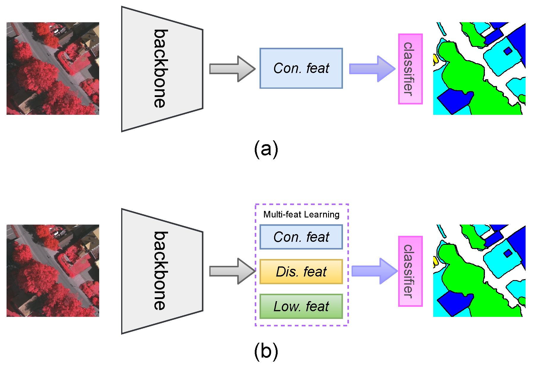
• We present a novel multi-feature learning mechanism that simultaneously learns con. feat, low. feat, and dis. feat to improve the performance of semantic segmentation.
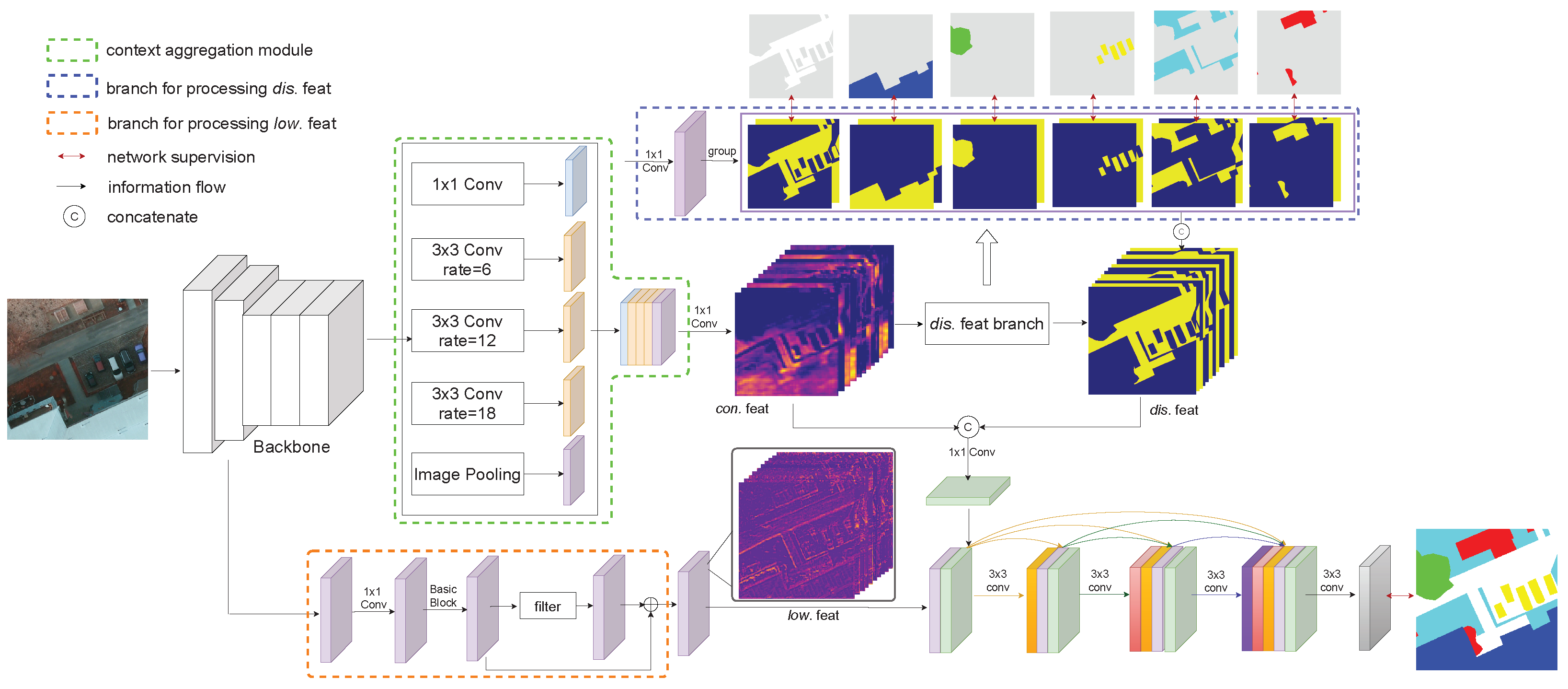
• Based on the above mechanism, we design a novel convolutional neural network framework (MFNet) for VHR RSI segmentation. Except for the context aggregation module for capturing con. feat, there is a branch for learning low. feat at the shallow layer in the backbone network through local contrast processing, and a branch for generating dis. feat with better inter-class discriminative capability via a class-specific group-optimized strategy.
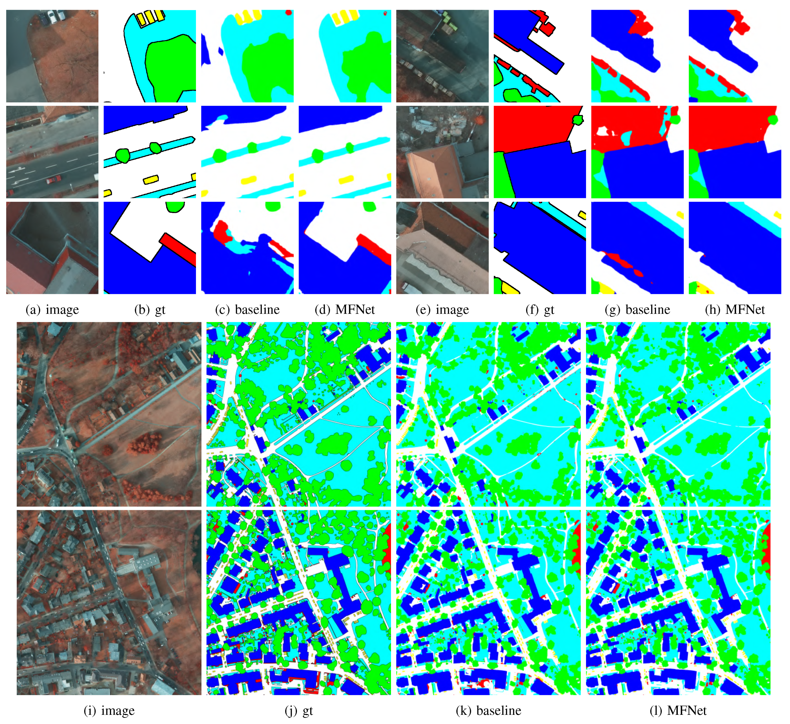
• We evaluate our proposed MFNet on two well-known VHR RSI benchmark datasets, the ISPRS Vaihingen and Potsdam datasets. Extensive experiments suggest that our proposed framework outperforms most cutting-edge models. In particular, we attain an overall accuracy score of 91.91% using only VGG16 [2] as the backbone on the Potsdam test set.

2. Related Works

Semantic Segmentation. In recent years, deep convolutional neural networks have made breakthroughs in the field of computer vision, such as image recognition (such as VGGNet [2], ResNet [3], DenseNet [22]), semantic segmentation (such as PSPNet [5], DeepLab [4,6], DANet [12], CCNet [13]), etc. The fully convolutional network [15], as a landmark work, first applied convolutional neural networks in image semantic segmentation. Due to the specificity of its application, remote sensing images usually have a very high resolution. Moreover, semantic segmentation requires more computational resources than other computer vision tasks because it must be analyzed at full resolution [1,11]. Therefore, it is impractical to perform semantic segmentation on VHR RSIs directly. From the perspective of the input image, there are two alternative solutions. One is to reduce the image resolution, and the other is to train based on a patch-based image. The former loses too much spatial information and has not been successful for VHR images, while the latter is the current solution for most VHR RSI segmentation models [7,8,10,11,23,24,25], and we are no exception. GLNet [1] integrated a global branch and a local branch to handle downsampled full-resolution images and cropped local patches at the same time in VHR RSIs, but the performance was poor. In addition, there are more patch-based segmentation models available, such as ScasNet [7], ResUNet-a [23], SCAttNet [24], etc. ScasNet [7] built an end-to-end self-ScasNet to improve the labeling coherence with sequential global-to-local context aggregation. ResUNet-a [23] adopted an architecture-based U-Net combined with residual connections, atrous convolutions, and pyramid scene parsing pooling to perform segmentation in VHR RSIs. SCAttNet [24] combined spatial and channel attention to improve the semantic segmentation accuracy of high-resolution remote sensing images. Yang et al. [8] leveraged a multi-path encoder structure for multi-path inputs and an attention-fused method to fuse high-level abstract features and low-level spatial features. Ding et al. [11] employed a two-stage multi-scale training architecture to better exploit the correlations between ground objects in VHR RSIs. However, most of the models listed above are devoted to capturing long-range contextual features through attention-based methods, or multi-scale designs, to improve model performance. Despite the good performance of these models, the problem of the semantic segmentation of VHR RSIs is still far from being solved, and it is worthwhile to further explore more complete features to drive the segmentation progress.

Feature Learning. Early feature learning approaches mainly used low-level, hand-crafted visual features to model semantic features on local parts of images (e.g., patches and super pixels). In the last decade, due to the development of deep learning, DCNNs have been shown to automatically and efficiently learn visual representations in computer vision tasks. In addition, a large number of deep learning models (such as VGG [2], ResNet [3], DenseNet [22], etc.) are used for feature extraction for downstream tasks (semantic segmentation [15] or object detection [26], for instance). In the case of semantic segmentation tasks, recent works have focused on extracting long-range contextual information, or multi-scale features to improve performance, since convolutional operation has only a limited receptive field in DCNNs when extracting features [4,5,6,12,13]. For example, DeepLab [4,6], as a classical semantic segmentation model, used atrous spatial pyramid pooling (ASPP) to capture the contextual information at multiple scales. PSPNet [5] of the same period adopted a spatial pyramid pooling module (SPP) to extract rich contextual information. With the rise of attention, attention-based approaches have also become popular. Mou et al. [27] produced a relation-augmented feature representation by learning and reasoning about global relationships via the spatial relation module and the channel relation module in VHR RSI segmentation. Self-attention [16] constructs a matrix of pairwise correlations between pixels to capture long-range contextual dependencies. Moreover, self-attention and its variants [13,17] are further applied in the field of semantic segmentation, and these contextual feature extraction methods are still suitable in our approach. Furthermore, the learning of low-level features is gradually attracting attention. DeepLabv3+ [6] designed a simple yet effective decoder to focus on low-level features, especially the features of object boundaries. Sun et al. [10] combined semantic information from deep layers and detailed information from shallow layers to enhance the results of FCNs [15]. GFFNet [28] imported low-level features to compensate for the lost detailed information in high-level features. Others [19,20] considered features that focus on edge understanding with local contrast information, which is a key aspect of low-level features. However, from the point of view of the feature learning, these approaches are not comprehensive enough; most of them only consider how to extract more effective contextual features, and a few of them consider introducing low-level features. In this work, we introduce a multi-feature learning mechanism to learn more complete features, including contextual features, low-level features, and class-specific discriminative features. After combining these three features, the performance of segmentation can be further improved.

3. Methodology

3.1. Overview

The proposed MFNet mainly consists of a backbone network and three parts to learn three different kinds of features, including contextual features (con. feat), low-level features (low. feat), and class-specific discriminative features (dis. feat). The overall architecture of the MFNet is illustrated in Figure 4. Our novelty lies in the development of a multi-feature learning mechanism, which learns these three different but complementary features and then combines them to improve the performance in the semantic segmentation of VHR RSIs. As stated in Section 2, our framework is also a patch-based classification, in which it will take in image patches extracted from VHR RSIs and output corresponding prediction maps.

3.2. Network Architecture

As demonstrated in Figure 4, we take an input image $I\in {\mathbb{R}}^{C\times H\times W}$, where C, H, and W indicate the number of channels, height, and width of image I, respectively. Without loss of generality, we choose ResNet50 [3] and VGG16 [2] as our backbone network to extract hierarchical features for MFNet, and the architectures of both backbone networks are illustrated in

Table 1. Backbone architecture.

(a) ResNet50
Layer Name	Output Size	50 Layer
conv1	$256\times 256$	$7\times 7$, 64, stride 2
conv2_x	$128\times 128$	$3\times 3$ max pool, stride 2
		$\left[\begin{array}{c}1\times 1,64\\ 3\times 3,64\\ 1\times 1,256\end{array}\right]\times 3$
conv3_x	$64\times 64$	$\left[\begin{array}{c}1\times 1,128\\ 3\times 3,128\\ 1\times 1,512\end{array}\right]\times 4$
conv4_x	$32\times 32$	$\left[\begin{array}{c}1\times 1,256\\ 3\times 3,256\\ 1\times 1,1024\end{array}\right]\times 6$
conv5_x	$16\times 16$	$\left[\begin{array}{c}1\times 1,512\\ 3\times 3,512\\ 1\times 1,2048\end{array}\right]\times 3$
		avgrage pool
	$1\times 1$	1000-d fc
		softmax
(b) VGG16
Layer Name	Output Size	16 Layer
		$3\times 3$, 64
conv1	$256\times 256$	$3\times 3$, 64
		$2\times 2$ max pool, stride 2
		$3\times 3$, 128
conv2_x	$128\times 128$	$3\times 3$, 128
		$2\times 2$ max pool, stride 2
conv3_x	$64\times 64$	$3\times 3$, 256
		$3\times 3$, 256
		$3\times 3$, 256
		$2\times 2$ max pool, stride 2
conv4_x	$32\times 32$	$3\times 3$, 512
		$3\times 3$, 512
		$3\times 3$, 512
		$2\times 2$ max pool, stride 2
conv5_x	$16\times 16$	$3\times 3$, 512
		$3\times 3$, 512
		$3\times 3$, 512
		$2\times 2$ max pool, stride 2
	$1\times 1$	4096-d fc
		4096-d fc
		1000-d fc
		softmax

. For ResNet50, we employ a pretrained residual network with the dilated strategy [5], which adopts dilated convolutions in the last two ResNet blocks. This enlarges the size of the final feature map to $\frac{1}{8}$ of the input image, while retaining more details without adding extra parameters. VGG16 [2], on the other hand, ignores this strategy in favor of maintaining its lightweight nature, with its last layer producing a feature map with a size of $\frac{1}{16}$ of the input image. Here, the output of the backbone network is $X\in {\mathbb{R}}^{C^{\prime }\times H^{\prime }\times W^{\prime }}$.

Next, we need to perform multi-feature learning, starting with the learning of con. feat. The conventional FCN [15] does not take into account the global context information, which helps to build associations among features to mitigate the effect of the limited receptive field in DCNNs. Therefore, to address this issue, we are prepared to leverage a context aggregation module to gather con. feat $F_{con}$. Although the context aggregation module is capable of capturing long-range contextual information, it often fails to distinguish the categories with similar appearances. In this case, extracting inter-class discriminative feature representation is critical to further improve the performance of semantic segmentation. Therefore, we append a branch on con. feat to learn dis. feat, which adopts the group-optimized strategy to improve the inter-class discriminative capability. More concretely, we group con. feat into N groups (N is the number of classes), and we then optimize the foreground and background of each class and finally concatenate the normalized class probability map as dis. feat $F_{dis}$. Integrating $F_{dis}$ into the network can significantly improve the inter-class discriminative capability of the network.

Furthermore, due to successive pooling or stride convolution, high-level features cause the loss of spatial detail information (e.g., object boundaries), whereas con. feat and dis. feat are learned based on high-level features that contain rich semantic information and do not address the loss of low-level spatial information. Therefore, we argue that the introduction of low. feat facilitates the recovery of spatial detail information in high-level features, which in turn improves the performance of semantic segmentation. Finally, we construct a network branch that leverages the local contrast processing [19,20,29] to obtain details of the high-frequency part of the shallow layer of the backbone network (i.e., the object boundaries), which can be considered as the low feat $F_{low}$, to help refine the spatial details in the predicted results.

Lastly, effectively integrating the learned features remains a key issue. In essence, both $F_{con}$ and $F_{dis}$ are built at the top of the backbone network and $F_{low}$ is learned from the shallow layer of the backbone network. In this work, we employ dense connection to integrate these features. The technique of dense connection can effectively integrate these features and share valuable information [22].

3.3. Contextual Feature

Since the convolution operation is only processed in a limited receptive field, it might cause intra-class discrepancies, which can affect the model’s performance. The introduction of multi-scale contextual information through the context aggregation module can broaden the receptive field and significantly improve the performance of the model [30]. In fact, our goal is to explore the effectiveness of con. feat in multi-feature learning. As far as feature learning is concerned, we are not bound to the form of the context aggregation module. To be more representative, we use the widely adopted atrous spatial pyramid pooling (ASPP) [4,6] for discussion, and we can also take another alternative form of self-attention [16].

Next, we elaborate the process to aggregate contextual information via atrous spatial pyramid pooling. Formally, given an output feature X from the backbone network, we first feed it into three parallel atrous convolutions with different atrous rates, resulting in a series of features $\{f_1,f_2,f_3\}$, where $f_i\in {\mathbb{R}}^{256\times H^{\prime }\times W^{\prime }}$. ASPP, with different atrous rates, effectively captures multi-scale information. Atrous convolution is applied over the input feature map X as follows:

$$f\left[p\right]=\sum _{k}X[p+r\ast k]w\left[k\right]$$

(1)

where p indicates the position in output feature f, w represents the weight of the convolutional layer, k is the kernel size, and r denotes the dilation rate.

Aside from the three parallel dilate convolutions, there is a stand convolution whose kernel size is $1\times 1$, to generate the feature $f_4$. According to [4], the image-level feature $f_5$ is produced by applying global average pooling on the same X, followed by a $1\times 1$ convolutional layer with 256 filters. Lastly, the features generated by all sub-branches are concatenated and then passed through another $1\times 1$ convolution (with batch normalization and ReLU) to generate the resulting feature $F_{con}$.

3.4. Class-Specific Discriminative Feature

Previous semantic segmentation models relying solely on con. feat for direct classification have achieved quite good results. However, this strategy usually fails to distinguish classes with similar appearances [14]. As a result, the addition of dis. feat with better inter-class discriminative capability is quite useful in distinguishing these confusing classes. Thus, a branch is built to learn dis. feat through a group-optimized strategy. This branch is based on the output feature $F_{con}$ of the context aggregation module. Moreover, learning dis. feat can also be directly based on the output of the backbone network, which can also achieve a certain degree of improvement. The reason that it is based on con. feat is to build on it and obtain further superior performance. What follows is a description of the process of learning dis. feat in great detail.

To begin, we apply a $1\times 1$ convolutional layer to map the con. feat $F_{con}$ to $F_{con}^{\prime }\in {\mathbb{R}}^{2C\times H^{\prime }\times W^{\prime }}$, where C is the number of classes in the dataset. After this, we group the feature $F_{con}^{\prime }$ into a set of group ${\left\{g_i\right\}}_{i=1,...,c}$. In our implementation, we split the feature map along the channel axis with a total of c groups corresponding to c classes, and each group $g_i$ is a 2-channel feature map, one of which is $g_i^{fg}$, and the other is $g_i^{bg}$. $fg$ denotes the foreground feature, while $bg$ is the background feature. Thus, we obtain better category distinctiveness by optimizing the foreground and background of each class separately. Such a class-specific group-optimized strategy was also adopted by [14,21]. Here, we set the predicted probability of each position o in each group $g_i$ as $p\left(o\right|g_i)$, and then its foreground probability $p_{i,o}^{fg}$ and background probability $p_{i,o}^{bg}$ are defined as follows:

$$\begin{array}{cc}\hfill p_{i,o}^{fg}& =p(o=1|g_i^{fg})\hfill \end{array}$$

(2)

$$\begin{array}{cc}\hfill p_{i,o}^{bg}& =p(o=0|g_i^{bg})\hfill \end{array}$$

(3)

Thus, the corresponding dis. feat map can be formulated as:

$$\begin{array}{cc}\hfill {\widehat{p}}_{i,o}^{fg}& =\frac{e^{p_{i,o}^{fg}}}{e^{p_{i,o}^{fg}}+e^{p_{i,o}^{bg}}}\hfill \end{array}$$

(4)

$$\begin{array}{cc}\hfill {\widehat{p}}_{i,o}^{bg}& =\frac{e^{p_{i,o}^{bg}}}{e^{p_{i,o}^{fg}}+e^{p_{i,o}^{bg}}}\hfill \end{array}$$

(5)

essentially, ${\widehat{p}}_{i,o}^{fg}$ and ${\widehat{p}}_{i,o}^{bg}$ are the normalized foreground and background probabilities, respectively. Finally, the resulting dis. feat $F_{dis}$ are defined as

$$F_{dis}=\mathcal{C}\left([{\widehat{p}}_{i,o}^{fg},{\widehat{p}}_{i,o}^{bg}]\right)$$

(6)

where the $\mathcal{C}$ is concatenated along the channel axis. Lastly, the corresponding multi-binary cross entropy loss is adopted to optimize $F_{dis}$, which can be formulated as follows:

$$\begin{array}{cc}\hfill {\mathcal{L}}_{dis}=& -\frac{1}{N}\sum _1^N\frac{1}{HW}\sum _{r=1}^{HW}\frac{1}{C}\sum _{i=1}^C[y\times log\left({\widehat{p}}_{i,o}^{fg}\right)\hfill \\ \hfill & +(1-y)\times log\left({\widehat{p}}_{i,o}^{bg}\right)].\hfill \end{array}$$

(7)

It should be noted that the foreground and background probability map of every group $g_i$ is equivalent to a binary prediction of the corresponding category. Moreover, they are obtained by optimization via binary cross-entropy (normalized by softmax). Therefore, the dis. feat can be viewed essentially as a multi-binary classification optimization result. In this way, the features of each category can be optimized separately, which is more conducive to distinguishing between confusing categories. Figure 5 visualizes a comparison of the effect of dis. feat and the dis. feat of corresponding categories.

3.5. Low-Level Features

Since high-level features are easily biased towards encoding features of large objects, spatial detail information is lost, leading to over-smoothed prediction results, especially along object boundaries [18]. Therefore, the introduction of low. feat containing rich spatial information is crucial to the performance of segmentation. Prior work has captured low. feat based on high-level features output by the backbone network [29]; however, this does not address the problem of low-level spatial information loss. This is due to successive convolution and pooling in feature extraction, which results in an over-smoothed high-level feature output. As a result of the over-smoothing, the degree of detail is reduced and the edges are unsharp, and no low-level spatial information can be accessed from the high-level features. As a consequence, we develop a branch to learn low. feat, mainly object boundary information, from the shallow layer in the backbone network, which can be utilized to recover the spatial details of the prediction results.

As we know, the feature map can be decomposed into a low-spatial-frequency component that depicts the smoothly changing structure, and a high-spatial-frequency component that represents the rapidly changing fine details, mainly object boundaries [31]. Inspired by [19,20,29], we apply the local contrast processing to learn the low. feat (mainly the object boundaries). This is accomplished by first obtaining local average features through average pooling layers, which can be interpreted as applying a low-pass filter to extract the low-frequency component, and then the remaining high-frequency part (i.e., low. feat) can be obtained by subtraction.

More specifically, taking an initial low. feat $x_l$ in the shallow layers from the backbone network, we first feed it into a $1\times 1$ convolution layer to reduce the dimensions of the feature. After this, a basic block [3] is employed to enhance the learning of object boundary features, which is an indispensable part of the process of learning low. feat. Its output is the feature $x_l^{\prime }$. Next, we define a local neighbor region R in $x_l^{\prime }$, where the size is set to 3 in this work. Then, we calculate the local average (smoothing) feature $x_{avg}^{\prime }$, which depends on neighbour region R in $x_l^{\prime }$, as shown in Equation (8):

$$x_{avg}^{\prime }=\frac{1}{R}\sum _{i\in R}{\left[x_l^{\prime }\right]}_i.$$

(8)

This operator is similar to the low-pass filter used for smoothing, which reduces the variance of the estimated value in the limited size of the neighborhood. In fact, thanks to this, we obtain the details of the remaining high-frequency part (such as object boundaries, etc.) by subtraction, which reveals the fine-grained details of $x_l^{\prime }$ as $x_{detail}^{\prime }$:

$$x_{detail}^{\prime }=x_l^{\prime }-x_{avg}^{\prime }.$$

(9)

The most significant part of the feature $x_{detail}^{\prime }$ is the object boundaries, which offer a strong spatial clue that helps to enforce the consistency of segmentation along the local object boundaries. Additionally, we add a shortcut connection [3] to the feature $x_{detail}^{\prime }$ such that the identity mapping can help to optimize the network and drive the learning of low. feat. Finally, the resulting low. feat can be defined as follows:

$$F_{low}=x_l^{\prime }+x_{detail}^{\prime }=2x_l^{\prime }-x_{avg}^{\prime }.$$

(10)

In this way, the network can produce sharper boundaries and fine-grained segmentation by incorporating low. feat that contain rich spatial information. Figure 6 demonstrates the effect of low. feat.

3.6. Dense Feature Aggregation

Con. feat $F_{con}$ and dis. feat $F_{dis}$ are based on high-level features, while the low. feat $F_{low}$ are learned from the shallow layers in the backbone network. However, aggregating three features via concatenating/summing directly may degrade the prediction performance. Consequently, we design a scheme of dense feature aggregation in order to fully exploit the strengths of each feature, to acquire valuable information and enhance the segmentation performance. First of all, con. feat $F_{con}$ and dis. feat $F_{dis}$ are concatenated together and passed through a $1\times 1$ convolutional layer to generate the resulting feature $F^c$. Then, we densely connect the feature $F_{low}$ and $F^c$, and the process is as follows:

$$\begin{array}{c}\hfill F_l=H_l\left([F_{low},F^c,F_1^c,\cdots ,F_{l-1}^c]\right)\end{array}$$

(11)

where $[F_1^c,\cdots ,F_{l-1}^c]$ refers to the combination of the feature maps produced in layer $0,\cdots ,l-1$, $H_l$ represent the l-th convolutional layer, and $F_l$ is the output of the l-th layer. The output of the last layer $F_l$ can be used for classification.

3.7. Loss

Our proposed MFNet utilizes multiple loss functions to optimize the learning process. Besides the widely used cross-entropy loss ${\mathcal{L}}_{ce}$, there is also the auxiliary loss ${\mathcal{L}}_{aux}$ proposed in PSPNet [5], which is well known in the field of semantic segmentation. It has been shown to bring a certain degree of improvement in the performance of the model. In addition, our method proposes a discriminative loss ${\mathcal{L}}_{dis}$ (i.e., Equation (7)) composed of multiple binary optimization losses.

Thus, the final loss function is as follows:

$$\begin{array}{cc}\hfill {\mathcal{L}}_{ce}& =-\sum _{i\in S}{y}_{i}log\left({\widehat{y}}_i\right)\hfill \end{array}$$

(12)

$$\begin{array}{cc}\hfill {\mathcal{L}}_{aux}& =-\sum _{i\in S^{\prime }}{y}_{i}log\left({\widehat{y}}_i^{\prime }\right)\hfill \end{array}$$

(13)

$$\begin{array}{cc}\hfill \mathcal{L}& ={\mathcal{L}}_{ce}+\alpha \ast {\mathcal{L}}_{aux}+\beta \ast {\mathcal{L}}_{dis},\hfill \end{array}$$

(14)

where $i\in S$ refers to a pixel in the output and ground truth, and $i\in S^{\prime }$ refers to a pixel in the auxiliary output and ground truth. y represents the ground truth, while $\widehat{y}$ is the model prediction; ${\widehat{y}}^{\prime }$ denotes the output of the auxiliary branch (i.e., another classifier is applied after the fourth stage, namely the res4b22 residual block). The auxiliary loss is also used as a common practice by numerous advanced models, such as PSPNet [5], CCNet [13], and DANet [12]. It helps to optimize the learning process, while the master branch loss takes the most responsibility. $\alpha$ and $\beta$ are weight parameters, and we empirically set $\alpha$ to 0.4 and $\beta$ to 1.0.

4. Description of Datasets and Design of Experiments

In this section, we firstly describe the datasets used in the experiments, including the ISPRS Potsdam dataset, Vaihingen dataset, and UAVid dataset [32]. Then, we provide the evaluation matrix for quantifying model performance, as well as experimental details concerning the parameters of the networks that are involved in our studies. Finally, we demonstrate the inference strategy regarding how to combine patch-based prediction results into full resolution.

4.1. Dataset Description

In order to analyze MFNet and evaluate its performance in VHR RSIs, we use three open benchmark datasets: the ISPRS Vaihingen dataset, Potsdam dataset, and UAVid dataset.

Vaihingen. The ISPRS Vahingen dataset [33] contains 33 large image patches. Each patch contains an orthorectified image tile (TOP) mosaic with three spectral bands (red, green, near-infrared), with a corresponding digital surface model (DSM) and normalized DSM (nDSM). The size of each patch is approximately $2500\times 2000$. The dataset has a ground sampling distance (GSD) of 9 cm. Moreover, it includes six categories: impervious surfaces, buildings, low vegetation, trees, cars, and clutter/background. Their corresponding colors have been defined in

Table 2. RGB values of the categories.

Category	RGB Value
Imp. Surf.	(255, 255, 255)
Building	(0, 0, 255)
Low veg.	(0, 255, 255)
Tree	(0, 255, 0)
Car	(255, 255, 0)
Clutter/background	(255, 0, 0)

. We divide the dataset into a training set and a test set according to the benchmark organizer. More specifically, the training set consists of 16 images and the remaining 17 patches are treated as the test set. It should be noted that we employ only TOP without DSM or nDSM in our experiments.

Potsdam. The ISPRS Potsdam dataset [34] is composed of 38 high-resolution image patches, each consisting of a true orthophoto extracted from a larger TOP mosaic, and with a corresponding DSM. The ground sampling distance of both the TOP and the DSM is 5 cm. All patches have a resolution of $6000\times 6000$ pixels. Each image contains four bands: near-infrared, red, green, and blue bands. It has the same categories as the ISPRS Vaihingen dataset. Although Potsdam offers more channels, we only use the same infrared–red–green (IRRG) images as Vaihingen in order to have a broader application. We adopt the official data split for the Potsdam dataset, where 24 training images are used for model construction and the remaining 14 test images are used for evaluation. DSM is also not used in this dataset.

UAVid. The UAVid dataset [32] is a high-resolution UAV video dataset for semantic segmentation tasks focusing on urban scenes. It has 300 images, each with a size of $4096\times 2160$ or $3840\times 2160$. Eight classes are selected for semantic segmentation, i.e., buildings, roads, trees, low vegetation, static cars, moving cars, humans, and clutter. We adopt the official data split for the UAVid dataset, i.e., 15 training sequences (150 labeled images) and 5 validation sequences (50 labeled images) for training and validation, respectively. The test split consists of the left 10 sequences (100 labeled images), whose labels are withheld for benchmarking purposes (the official benchmark can be seen at https://uavid.nl, accessed on 15 December 2021).

4.2. Evaluation Metrics

To comprehensively evaluate our proposed model, we use three evaluation metrics, namely the mean intersection over union (mIoU), mean ${\mathrm{F}}_1$ score (mF1), and overall accuracy (OA), to evaluate the semantic segmentation performance. They are defined as:

$$\begin{array}{cc}\hfill {\mathrm{F}}_1& =\frac{2\mathrm{TP}}{2\mathrm{TP}+\mathrm{FP}+\mathrm{FN}}\hfill \end{array}$$

(15)

$$\begin{array}{cc}\hfill \mathrm{OA}& =\frac{\mathrm{TP}+\mathrm{TN}}{\mathrm{TP}+\mathrm{FP}+\mathrm{TN}+\mathrm{FN}}\hfill \end{array}$$

(16)

$$\begin{array}{cc}\hfill \mathrm{IoU}& =\frac{\mathrm{TP}}{\mathrm{TP}+\mathrm{FP}+\mathrm{FN}}\hfill \end{array}$$

(17)

in which TP, TN, FP, and FN are the number of true positives, true negatives, false positives, and false negatives, respectively.

Notably, the overall accuracy is computed for all categories including the background for a comprehensive comparison with different models. Moreover, the evaluation is carried out using ground truth with eroded boundaries provided in the datasets following previous studies [35]. It should be noted that, following the official benchmark, the class clutter/background is not included in the computation of mIoU and mF1 because its proportion is very low (as illustrated in Figure 7) and it is insignificant in practice.

4.3. Implementation Details

Our model is implemented on PyTorch. We use the mini-batch Stochastic Gradient Descent (SGD) optimizer with an initial learning rate of 0.001, momentum of 0.9, and a weight decay of 0.0001. Similar to [25], we employ the “poly” learning rate policy, where the learning rate is multiplied by ${(1-\frac{iter}{ite{r}_{max}})}^{0.9}$. Our experiments are conducted for 50 epochs on a single NVIDIA-3090 and the batch size is set to 4. Considering the limited GPU memory, we crop each patch into $512\times 512$ from full-resolution images using a sliding window with 171 px ($512\times \frac{1}{3}$) stride. Common data augmentation methods are performed to avoid over-fitting, including random flipping. For semantic segmentation, we choose FCN [15] pretrained on ImageNet as our baseline (VGG16 as the backbone network), and we also utilize ResNet50 to further verify the robustness and validity of our proposed method.

4.4. Inference Strategy

In evaluation mode, we perform inference using the sliding window test by cropping $512\times 512$ windows with 171 px stride. However, pixels near the boundaries are not classified with as much confidence as pixels near the center, because the center pixels have more contextual information [23]. As a matter of fact, the contextual information of boundaries pixels is finite since there is no information outside the boundaries of the image patches. Therefore, to further improve the performance of the model and provide seamless segmentation masks, the inference is enhanced with multiple overlapping inference windows. Moreover, this strategy is widely used in high-resolution image semantic segmentation, as in Cityscapes [36].

5. Experimental Results

We first carry out experiments on the Vaihingen dataset, which is a widely used benchmark for VHR RSI segmentation. After image patch extraction, it has a total of 1103 images with a size of $512\times 512$. Nonetheless, it can only be considered a small dataset. For a better and more comprehensive evaluation of our algorithm, we also test it on the Potsdam dataset, which is a large-scale benchmark consisting of more than 10,000 images. It is worth noting that we aim to perform a comprehensive and detailed evaluation of the proposed MFNet, unlike previous approaches that only validate using a single backbone. Here, we present the evaluation results for both the ResNet50 and VGG16 backbones.

5.1. Experiments on Vaihingen

5.1.1. Ablation Study of Multi-Feature Learning

In this section, we explore the effect of multi-feature learning in the proposed framework. It learns more complete features, including contextual features (con. feat), class-specific discriminative features (dis. feat), and low-level features (low. feat), to improve model performance. Based on the baseline (i.e., FCN), we build various networks depending on different features and their combinations to validate the performance of corresponding features.

Table 3. The result of ablation study of multi-feature learning in Vaihingen dataset.

Backbone	Model	Imp. Surf.	Building	Low Veg.	Tree	Car	mF1(%)	mIoU(%)	OA(%)
VGG16	FCN	90.61	93.82	82.08	89.03	72.43	85.59	75.56	88.96
	+low.	91.55	94.25	83.37	89.44	84.39	88.60	79.78	89.78
	+dis.	91.12	84.11	81.89	88.83	76.65	86.52	76.79	89.13
	+con.	90.97	94.10	82.65	89.15	74.68	86.31	76.55	89.28
	+low.+dis.	91.84	94.59	82.92	89.42	86.47	89.05	80.50	89.90
	+con.+low.	92.03	94.67	83.41	89.56	85.40	89.01	80.45	90.09
	+con.+dis.	91.71	94.61	82.70	89.29	78.17	87.30	77.96	89.70
	+con.+dis.+low.	92.31	95.06	83.45	89.74	85.59	89.23	80.82	90.36
Res50	FCN	92.06	95.27	83.74	89.61	84.96	89.13	80.66	90.36
	+low.	92.21	95.21	83.69	89.68	87.30	89.62	81.42	90.40
	+dis.	92.45	95.41	83.85	89.56	86.82	89.62	81.44	90.51
	+con.	92.23	95.51	83.92	89.77	84.94	89.27	80.91	90.54
	+low.+dis.	92.70	95.68	83.53	89.54	87.86	89.86	81.85	90.64
	+con.+low.	92.33	95.58	83.92	89.89	86.18	89.58	81.39	90.62
	+con.+dis.	92.84	95.70	84.04	89.67	87.50	89.95	81.99	90.77
	+con.+dis.+low.	92.93	95.77	84.08	89.80	88.49	90.21	82.41	90.89

reports the results of the experiments of multi-feature learning. As shown in Table 3, our multi-feature learning scheme achieves a significant improvement, and all three features learned have a certain degree of gain over the baseline. In particular, our model gains 1.4% with VGG16 as the backbone when learning the three features together. Moreover, multi-feature learning is capable of demonstrating its superiority even against a stronger baseline (i.e., Dilated FCN [5] with ResNet50)). Furthermore, when all features are learned at the same time, it performs better than learning a single feature. This shows that the three features we learned are complementary. Next, we analyze the roles of individual features.

The effect ofcon. feat. We employ ASPP [6] as the context aggregation module at the top of the backbone network to capture long-range dependencies for improved semantic segmentation. In fact, the context aggregation module is mainly used to capture con. feat, independent of its specific form. Although we adopt ASPP, other comparable modules, such as self-attention (SA) [16], PPM [5], CGNL [17], etc., can also improve the performance of the baseline.

Table 4. Comparison with different context aggregation modules in vaihingen dataset.

Backbone	Method	mF1(%)	mIoU(%)	OA(%)
VGG16	FCN (baseline)	85.59	75.56	88.96
	+ASPP [6]	86.31	76.55	89.28
	+PPM [5]	85.43	75.44	89.14
	+SA [16]	85.77	75.77	88.96
	+CGNL [17]	85.82	75.92	89.20
	+CC [13]	87.77	75.82	89.10
Res50	FCN (baseline)	89.13	80.66	90.36
	+ASPP [6]	89.27	80.91	90.54
	+PPM [5]	89.27	80.91	90.53
	+SA [16]	89.03	80.52	90.26
	+CGNL [17]	88.88	80.31	90.36
	+CC [13]	89.10	80.61	90.23

reports the results of the ablation study on the context aggregation module. Moreover, we can observe that all of the methods listed in Table 4 have been improved over the baseline, with ASPP achieving good performance whether they were based on VGG16 or ResNet50.

The effect ofdis. feat. The dis. feat are an indispensable feature, but they have often been ignored by models that rely solely on con. feat $F_{con}$. Looking at the performance of the baseline model with only dis. feat in Table 3, although our dis. feat still demonstrate a gain on FCN (OA value of 0.17%), this gain is much lower than that of the other two features (OA value of 0.32% and 0.82%, respectively), especially on the model with VGG16 as the backbone. This is mainly because our dis. feat need to be built on high-level features, and VGG16, as an early deep convolutional network, is insufficient to provide higher-level deep features for the segmentation model. Nevertheless, if the learning is based on con. feat, the effect is significant. More specifically, as far as OA is concerned, compared to using only the dis. feat, dis. + con. feat yields an improvement of nearly 1%, as can be seen from Table 3. In addition, thanks to the deeper network to extract richer semantic information, the network with dis. feat performs better on ResNet50 than on VGG16, both for single dis. feat and for the combination of dis. feat.

The effect oflow. feat.low. feat is essential for recovering detailed spatial information. The advanced model DeepLabv3+ [6] adopted a simple decoder to learn low-level features. However, the decoder adopted by DeepLabv3+ does not demonstrate an advantage in the context of VHR RSIs. The combination of low. feat and con. feat captured by ASPP allows it to achieve the best performance in the task of natural image segmentation. It outperforms DeepLabv3 [4], which relies only on con. feat. Our proposed low. feat learning branch improves the performance of segmentation by 0.82% (OA in VGG16) over the baseline by learning low-level features, as stated in Table 3. Therefore, it can be seen that, in the case of VGG16 as the backbone network, low. feat contribute more to the model performance than the other two types of features. In addition, the low. feat also provide a consistent improvement in model performance in the case of ResNet50.

Feature aggregation. In fact, the low. feat cannot be simply combined with the con. and dis. feat constructed based on the high-level features. DeepLabv3+ adopted a concatenated method to combine low. feat and con. feat. However, this combination ignores the essential difference between the two features. One is mainly spatial detail information, and the other is high-level semantic features. We use dense connection to aggregate these features and address this problem, and the corresponding experimental results are shown in

Table 5. Comparison of the method of concatenation (cat) and dense connection (dense) in Vaihingen dataset.

Backbone	Model	mF1(%)	mIoU(%)	OA(%)
VGG16	cat	88.78	80.11	90.23
	dense	89.23	80.82	90.36
Res50	con	90.04	82.13	90.80
	dense	90.21	82.41	90.89

. The experimental results verify the effectiveness of the dense connection scheme.

5.1.2. Ablation Study for Improvement Strategies

Following [12,35], we also adopt some common strategies to improve the performance further. (1) DA: Data augmentation with random scaling (from 0.5 to 1.5). (2) Multi-Grid (MG): We employ a hierarchy of grids of different sizes (4, 8, 16) in the last ResNet block. It should be noted that this strategy was not applied in VGG16. (3) Multi-Scale (MS): We average the segmentation probability maps from 5 scales $\{0.5,0.75,1.0,1.25,1.5\}$ for inference. Experimental results are shown in

Table 6. Performance comparison between different improvement strategies on Vaihingen dataset.

Backbone	DA	MG	MS	Imp. Surf.	Building	Low Veg.	Tree	Car	mF1(%)	mIoU(%)	OA(%)
VGG16				92.31	95.06	83.45	89.74	85.59	89.23	80.82	90.36
	✓			92.36	95.42	84.01	89.88	84.60	89.25	80.88	90.61
	✓	-		-	-	-	-	-	-	-	-
	✓	-	✓	92.78	95.57	85.08	90.52	84.38	89.67	81.55	91.11
Res50				92.93	95.77	84.08	89.80	88.49	90.21	82.41	90.89
	✓			93.03	96.01	84.58	90.08	87.71	90.28	82.53	91.13
	✓	✓		93.23	96.19	85.12	90.03	87.85	90.48	82.86	91.32
	✓	✓	✓	93.43	96.35	85.85	90.50	88.31	90.88	83.50	91.67

. Data augmentation does not show significant improvements on mF1 and mIoU, but achieves some improvement on OA, both on VGG16 and ResNet50. We adopt MG to obtain better feature representations of the pretrained network, which further achieves a 0.13% improvement on ResNet50. Finally, the multiple segmentation map fusion strategy further improves the performance to 91.11% and 91.68% on VGG16 and ResNet50, respectively.

5.1.3. Results on Vaihingen Dataset

We further compare our method with the state-of-the-art methods on the Vaihingen dataset. Results are listed in

Table 7. Comparisons with state-of-the-art on Vaihingen test set.

Method	Backbone	Imp. Surf.	Building	Low Veg.	Tree	Car	mF1(%)	mIoU(%)	OA(%)
FCN [15]	VGG16	88.67	92.83	76.32	86.67	74.21	83.74	72.69	86.51
UZ_1 [37]	-	89.20	92.50	81.60	86.90	57.30	81.50	-	87.30
RoteEqNet [38]	-	89.50	94.80	77.50	86.50	72.60	84.18	-	87.50
S-RA-FCN [39]	VGG16	91.47	94.97	80.63	88.57	87.05	88.54	79.76	89.23
UFMG_4 [40]	-	91.10	94.50	82.90	88.80	81.30	87.72	-	89.40
V-FuseNet [41]	-	92.00	94.4	84.50	89.90	86.30	89.42	-	90.00
DLR_9 [42]	-	92.40	95.20	83.90	89.90	81.20	88.52	-	90.30
TreeUNet [43]	-	92.50	94.90	83.60	89.60	85.90	89.30	-	90.40
DANet [12]	ResNet101	91.63	95.02	83.25	88.87	87.16	89.19	81.32	90.44
DeepLabv3+ [6]	ResNet101	92.38	95.17	84.29	89.52	86.47	89.57	81.47	90.56
PSPNet [5]	ResNet101	92.79	95.46	84.51	89.94	88.61	90.26	82.58	90.85
ACFNet [44]	ResNet101	92.93	95.27	84.46	90.05	88.64	90.27	82.68	90.90
BKHN11	ResNet101	92.90	96.00	84.60	89.90	88.60	90.40	-	91.00
CASIA2 [7]	ResNet101	93.20	96.00	84.70	89.90	86.70	90.10	-	91.10
CCNet [13]	ResNet101	93.29	95.53	85.06	90.34	88.70	90.58	82.76	91.11
MFNet (Ours)	VGG16	92.78	95.57	85.08	90.52	84.38	89.67	81.55	91.11
MFNet (Ours)	ResNet50	93.43	96.35	85.85	90.50	88.31	90.88	83.50	91.67

. MFNet outperforms existing approaches with a dominant advantage. Specifically, MFNet with ResNet50 achieves 91.67% OA, outperforming prior work by a large margin. Moreover, the top performance of 91.11% OA was achieved merely using a small backbone network—VGG16. Such performance is further proof of the effectiveness and superiority of our proposed multi-feature learning strategy. In addition, qualitative results are presented in Figure 8. As shown in the figure, MFNet produces better segmentation maps than the baseline.

5.2. Experiments on Potsdam

5.2.1. Ablation Study of Multi-Feature Learning

Here, we explore the multi-feature learning scheme on the Potsdam dataset. The experimental set is the same as that for the Vaihingen dataset. The results of the ablation study on the Potsdam dataset are listed in

Table 8. The results of ablation study of multi-feature learning on Potsdam dataset.

Backbone	Model	Imp. Surf.	Building	Low Veg.	Tree	Car	mF1(%)	mIoU(%)	OA(%)
VGG16	FCN	92.47	96.10	86.41	87.93	94.79	91.52	84.59	90.06
	+low.	92.72	96.37	86.88	88.09	96.17	92.05	85.52	90.35
	+dis.	92.70	96.45	86.97	88.56	94.56	91.85	85.12	90.52
	+con.	93.13	96.75	87.29	88.40	95.27	92.17	85.69	90.88
	+low.+dis.	93.06	96.62	87.23	88.26	96.02	92.24	85.83	90.71
	+con.+low.	93.39	96.99	87.26	88.69	96.16	92.50	86.29	91.02
	+con.+dis.	93.49	97.15	87.53	88.31	95.57	92.41	86.12	91.14
	+con.+dis.+low.	93.55	97.12	87.49	88.53	96.17	92.57	86.42	91.25
Res50	FCN	93.55	97.08	87.16	88.45	96.31	92.51	86.33	91.04
	+low.	93.50	96.92	87.46	88.95	96.19	92.60	86.46	91.16
	+dis.	93.56	97.17	87.50	88.93	96.39	92.71	86.65	91.20
	+con.	93.71	97.15	87.75	88.98	96.25	92.77	86.74	91.38
	+low.+dis.	93.63	97.17	87.58	88.55	96.41	92.67	86.59	91.22
	+con.+low.	93.59	97.09	88.02	89.28	96.14	92.82	86.82	91.49
	+con.+dis.	93.83	97.33	87.72	88.92	96.74	92.91	87.01	91.47
	+con.+dis.+low.	93.92	97.40	87.83	88.99	96.69	92.96	87.10	91.61

. As stated in Table 8, our multi-feature learning mechanism remains effective on the larger-scale Potsdam dataset. Moreover, thanks to the larger amount of data and more complete features learned, the performance gap between the models with ResNet50 and VGG16 as the backbone is smaller. In particular, the performance gap between these two backbone networks (in terms of OA) is 0.53% on Vaihingen and 0.36% on Potsdam. This suggests, to some extent, that even a small backbone can be learned quite well if the features are learned properly.

The effect ofcon.feat. Unlike the experimental results for Vaihingen, the effect of con. feat is more significant and far exceeds the effect exerted by the other two features on the Potsdam dataset. Specifically, the baseline with con. feat gained 0.82% in terms of OA for Potsdam, while the other two combined features did not reach this value.

Table 9. Comparison of the performance with different context aggregation modules for Potsdam dataset.

Backbone	Method	mF1(%)	mIoU(%)	OA(%)
VGG16	FCN(baseline)	91.52	84.59	90.06
	+ASPP [6]	92.17	85.69	90.88
	+PPM [5]	92.04	85.47	90.80
	+SA [16]	92.12	85.59	90.95
	+CGNL [17]	92.17	85.70	90.85
	+CC [13]	91.88	85.19	90.67
Res50	FCN(baseline)	92.51	86.33	91.04
	+ASPP [6]	92.77	86.74	91.38
	+PPM [5]	92.66	86.57	91.24
	+SA [16]	92.49	86.29	91.25
	+CGNL [17]	92.54	86.35	91.29
	+CC [13]	92.66	86.55	91.30

shows the performance of different context aggregation modules appended in our baseline on Potsdam. The results are in accordance with those shown for the Vaihingen dataset. All of the context aggregation modules improve the baseline performance in a positive way, which indicates that our multi-feature learning framework is not restricted by the form of learning con. feat, but rather focuses more on the features themselves.

The effect ofdis. feat.dis. feat is also not negligible on the Potsdam dataset. Additionally, dis. feat had a better effect on high-level features. If it is attached directly at the top of the backbone network, it will only provide a minor improvement (0.46% in terms of OA with VGG16, while the value is 0.16% in ResNet50). However, when coupled with con. feat, it can work in its favor and offer comparable performance (the gain of OA is up to 1% with VGG16) as for the Vaihingen dataset. Nevertheless, this does not negate the fact that it is one of the most significant factors in determining performance.

The effect oflow. feat.low. feat still performs well on Potsdam. Furthermore, although it lags behind the other two features in terms of performance in the experiments with independent features (for example, the gain of OA is 0.29% with VGG16, while the values for the other two features are 0.46% and 0.82%, respectively), when combined with con. feat, it surpasses other combinations of two features, particularly in the network with ResNet50 as the backbone. More specifically, as stated in Table 8, low. feat + con. feat surpasses the other two combinations by 91.49% (value of OA).

Feature aggregation. We conduct relevant experiments on how to integrate low. feat with the other two high-level features. The results are presented in

Table 10. Comparison of the methods of concatenation (cat) and dense connection (dense) for Potsdam dataset.

Backbone	Model	mF1(%)	mIoU(%)	OA(%)
VGG16	cat	92.55	86.39	91.14
	dense	92.57	86.42	91.25
Res50	cat	92.90	87.01	91.46
	dense	92.96	87.10	91.61

. Concatenation and dense connection are the primary comparisons. Moreover, we come to the same conclusion as for Vaihingen based on the results in Table 10.

5.2.2. Ablation Study for Improvement Strategies

Here, we adopt three improvement strategies, including DA, MG, and MS, which are also applied to the Vaihingen dataset.

Table 11. Performance comparison between different improvement strategies on Potsdam dataset.

Backbone	DA	MG	MS	Imp. Surf.	Building	Low Veg.	Tree	Car	mF1(%)	mIoU(%)	OA(%)
VGG16				93.55	97.12	87.49	88.53	96.17	92.57	86.42	91.25
	✓			93.82	97.33	87.93	88.83	96.21	92.82	86.84	91.56
	-	-	-	-	-	-	-	-	-	-	-
	✓	-	✓	94.09	97.43	88.49	89.29	96.40	93.14	87.38	91.91
Res50				93.92	97.40	87.83	88.99	96.69	92.96	87.10	91.61
	✓			94.02	97.22	87.99	89.08	96.34	92.93	87.02	91.68
	✓	✓		94.27	97.41	88.05	89.06	96.57	93.07	87.28	91.82
	✓	✓	✓	94.25	97.52	88.42	89.43	96.62	93.25	87.57	91.96

reports the experimental results with all of the improvement strategies. From Table 11, we can find that each improvement strategy yields a different level of improvement. Additionally, there is a surprising result wherein the network with VGG16 as the backbone has an OA (the value of 91.91%) comparable to that (the value of OA is 91.96%) of the network with ResNet50 as the backbone after using the improvement strategies. On the one hand, this affirms the effectiveness of the improvement strategies, and on the other hand, this is a good indication that the multi-feature learning of our network can achieve excellent performance without using a large backbone. It should be noted that these improvement strategies are some general practices that are not specific to our network and are widely adopted by other approaches [12,35].

5.2.3. Results for Potsdam Dataset

Finally, we compare our method with several state-of-the-art methods on the Potsdam dataset. Numerical comparisons with state-of-the-art methods are listed in

Table 12. Comparisons with state-of-the-art on Potsdam test set.

Method	Backbone	Imp. Surf.	Building	Low Veg.	Tree	Car	mF1(%)	mIoU(%)	OA(%)
FCN [15]	VGG16	88.61	93.29	83.29	79.83	93.02	87.61	78.34	85.59
UZ_1 [37]	-	89.30	95.40	81.80	80.50	86.50	86.70	-	85.80
UFMG_4 [40]	-	90.80	95.60	84.40	84.30	92.40	89.50	-	87.90
S-RA-FCN [39]	VGG16	91.33	94.70	86.81	83.47	94.52	90.17	82.38	88.59
V-FuseNet [41]	-	92.70	96.30	87.30	88.50	95.40	92.04	-	90.60
TSMTA [11]	ResNet101	92.91	97.13	87.03	87.26	95.16	91.90	-	90.64
Multi-filter CNN [45]	VGG16	90.94	96.80	76.32	73.37	88.55	85.23	-	90.65
TreeUNet [43]	-	93.10	97.30	86.60	87.10	95.80	91.98	-	90.70
DeepLabv3+ [6]	ResNet101	92.95	95.88	87.62	88.15	96.02	92.12	84.32	90.88
CASIA3 [7]	ResNet101	93.40	96.80	87.60	88.30	96.10	92.44	-	91.00
PSPNet [5]	ResNet101	93.36	96.97	87.75	88.50	95.42	92.40	84.88	91.08
BKHN3	ResNet101	93.30	97.20	88.00	88.50	96.00	92.60	-	91.10
AMA_1	-	93.40	96.80	87.70	88.80	96.00	92.54	-	91.20
CCNet [13]	ResNet101	93.58	96.77	86.87	88.59	96.24	92.41	85.65	91.47
HUSTW4 [46]	-	93.60	97.60	88.50	88.80	94.60	92.62	-	91.60
SWJ_2	ResNet101	94.40	97.40	87.80	87.60	94.70	92.38	-	91.70
MFNet(Ours)	VGG16	94.09	97.43	88.49	89.29	96.40	93.14	87.38	91.91
MFNet(Ours)	ResNet50	94.25	97.52	88.42	89.43	96.62	93.25	87.57	91.96

. There is no doubt that our model far surpasses the previous state-of-the-art models. Furthermore, almost all the advanced models use the larger ResNet101 as the backbone network to obtain better performance. This is mainly due to the fact that deeper models can greatly increase the feature representation and generalization capabilities. However, thanks to the multi-feature learning mechanism, which provides a more complete feature representation, we can achieve considerable performance with only a small model (i.e., VGG16) as the backbone network. Figure 9 visualizes the segmentation results of several images in the Potsdam dataset. According to the figure, our proposed MFNet is closer to the ground truth than the baseline.

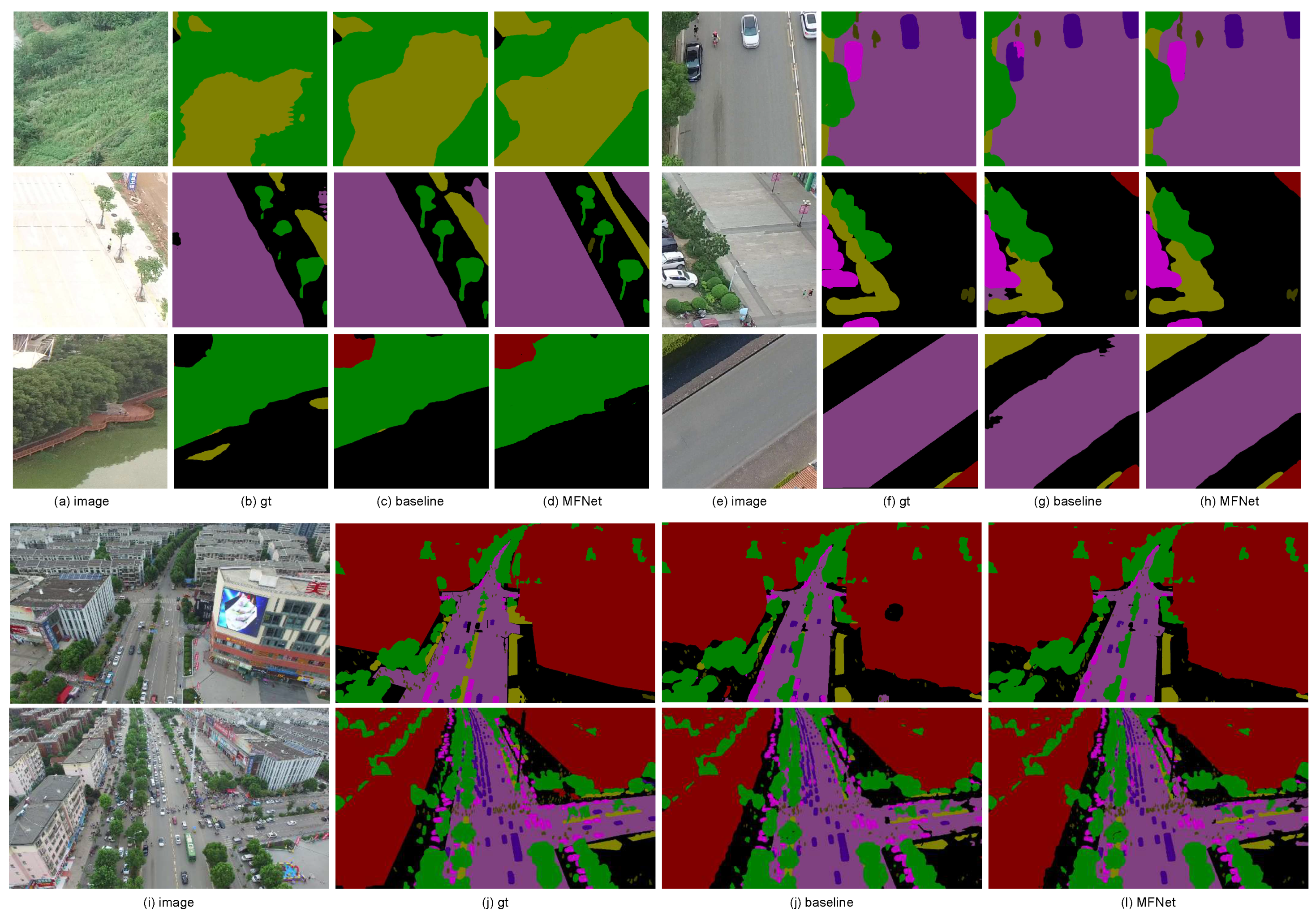
5.3. Experiments on UAVid

To verify the validity of the proposed model, we further conduct experiments on the more challenging UAVid dataset. This dataset is more difficult than the previous two datasets because the scenes captured by the UAVs are more complex and the number of categories is relatively high, with up to eight categories. Numerical comparisons with state-of-the-art methods are listed in

Table 13. Comparisons with state-of-the-art on UAVid test set.

Methods	Class IoU(%)								mIoU (%)	OA(%)
	Clutter	Building	Road	Tree	Low Veg.	Mov. Car	Sta. Car	Human
Dilation Net [30]	45.40	80.70	65.10	73.80	45.50	53.60	24.50	0.00	48.60	-
FCN-8s [15]	63.91	84.72	76.51	78.32	61.88	65.87	45.54	22.26	62.38	84.55
SegNet [47]	65.62	85.89	79.23	78.78	63.73	68.94	52.10	19.29	64.20	85.54
U-Net [48]	61.80	82.94	75.15	77.27	62.03	59.59	29.98	18.62	58.42	83.43
MSD [32]	57.00	79.80	74.00	74.50	55.90	62.90	32.10	19.70	57.00	-
ERFNet [49]	64.50	85.58	77.34	77.87	62.21	60.64	46.13	0.00	59.28	84.69
BiSeNetV2 [50]	61.18	81.62	77.11	75.97	61.30	66.36	38.51	15.40	59.68	83.10
ABCNet [51]	67.44	86.43	81.24	79.92	63.10	69.84	48.42	13.91	63.79	86.25
DANet [12]	64.85	85.88	77.94	78.29	61.47	59.64	47.44	9.14	60.58	84.99
MANet [52]	64.46	85.37	77.81	76.98	60.33	67.18	53.61	14.89	62.58	84.48
BANet [53]	66.66	85.38	80.71	78.87	62.09	69.32	52.83	21.03	64.61	85.73
A2-FPN [54]	67.37	87.20	80.16	80.11	63.73	70.14	53.33	23.43	65.68	86.35
PSPNet [5]	68.89	87.96	82.20	81.07	65.69	70.30	56.31	24.67	67.13	87.28
DeepLabV3 [4]	69.70	88.50	82.10	80.23	65.76	71.75	61.43	21.37	67.60	87.27
DeepLabV3+ [6]	68.86	87.62	82.22	79.76	65.88	69.86	55.39	26.07	66.96	86.94
MFNet(VGG16)	68.62	87.64	81.97	81.43	66.84	72.60	55.16	23.13	67.17	87.33
MFNet(ResNet50)	69.66	88.63	82.51	81.31	66.42	73.21	60.59	27.44	68.72	87.63

. It can be seen that our proposed MFNet with Resnet50 achieves the highest mIoU of 68.72%, and an OA of 87.63%, which surpass the results of other advanced models (such as PSPNet [5], DeepLabV3 [4]). Some visualized results of MFNet on the UAVid validation set are shown in Figure 10. The segmentation maps produced by MFNet are more precise and accurate than the baseline.

5.4. Computational Complexity

We compare the computational complexity with state-of-the-art methods, e.g., DeepLab V3/V3+ [4,6], DANet [12], and CCNet [13]. Model parameters and computation FLOPs are also listed for comparison in

Table 14. Computational complexity.

Model	Backbone	Params (M)	Macs (G)	FPS
FCN [15]	VGG16	15.90	38.62	69.63
DeepLab V3 [4]	ResNet50	42.12	85.44	16.47
DeepLab V3+ [6]	ResNet50	42.83	94.41	16.27
PSPNet [5]	ResNet50	68.06	128.66	20.09
Non-local [16]	ResNet50	54.75	110.96	23.29
CCNet [13]	ResNet50	35.76	74.14	22.83
CGNL [17]	ResNet50	36.26	75.09	19.45
DANet [12]	ResNet50	49.92	101.56	19.34
MFNet	VGG16	18.86	51.37	46.01
MFNet	ResNet50	49.88	133.73	13.36

. Notely, for a fair comparison, we use the same backbone network to evaluate the computational complexity. As can be seen from the table, our model with ResNet50 as the backbone does not have a significant advantage in terms of computational complexity, despite achieving the most advanced performance. However, thanks to our multi-feature learning mechanism, our model with VGG16 as the backbone has a significant advantage in terms of both time complexity and computational complexity, while achieving similar results as the ResNet50 backbone model (detailed performance is listed in Table 7 and Table 12).

6. Conclusions

In this paper, we propose a novel multi-feature learning framework for the semantic segmentation of VHR RSIs, which consists of a backbone network and three parts for learning three kinds of features, including contextual features, class-specific discriminative features, and low-level features. Contextual features have been the focus of previous work and are an integral part of our work. However, we are not bound to this form and we aim to leverage it to improve the performance of semantic segmentation. Furthermore, we further explore class-specific discriminative features to reduce misclassification due to similarity or a lack of significant differences. In addition, the introduction of low-level features can help the model to recover spatial detail information. The joint learning of the three features significantly enhances the performance of the semantic segmentation of VHR RSIs, and extensive experiments on the Vaihingen and Potsdam benchmarks demonstrate the effectiveness and superiority of the proposed MFNet. Our next work will focus on the design of lightweight neural networks using the multi-feature learning mechanism, which can be applied to applications that require a combination of speed and accuracy, such as Unmanned Aerial Vehicle (UAV) Remote Sensing.

References

1. Chen, W.; Jiang, Z.; Wang, Z.; Cui, K.; Qian, X. Collaborative global-local networks for memory-efficient segmentation of ultra-high resolution images. In Proceedings of the IEEE/CVF Conference on Computer Vision and Pattern Recognition, Long Beach, CA, USA, 15–20 June 2019; pp. 8924–8933. [Google Scholar]
2. Simonyan, K.; Zisserman, A. Very Deep Convolutional Networks for Large-Scale Image Recognition. In Proceedings of the International Conference on Learning Representations, San Diego, CA, USA, 7–9 May 2015. [Google Scholar]
3. He, K.; Zhang, X.; Ren, S.; Sun, J. Deep residual learning for image recognition. In Proceedings of the IEEE Conference on Computer Vision and Pattern Recognition, Las Vegas, NV, USA, 27–30 June 2016; pp. 770–778. [Google Scholar]
4. Chen, L.; Papandreou, G.; Schroff, F.; Adam, H. Rethinking atrous convolution for semantic image segmentation. arXiv 2017, arXiv:1706.05587. [Google Scholar]
5. Zhao, H.; Shi, J.; Qi, X.; Wang, X.; Jia, J. Pyramid scene parsing network. In Proceedings of the IEEE Conference on Computer Vision and Pattern Recognition, Honolulu, HI, USA, 21–26 July 2017; pp. 2881–2890. [Google Scholar]
6. Chen, L.; Zhu, Y.; Papandreou, G.; Schroff, F.; Adam, H. Encoder-decoder with atrous separable convolution for semantic image segmentation. In Proceedings of the European Conference on Computer Vision (ECCV), Munich, Germany, 8–14 September 2018; pp. 801–818. [Google Scholar]
7. Liu, Y.; Fan, B.; Wang, L.; Bai, J.; Xiang, S.; Pan, C. Semantic labeling in very high resolution images via a self-cascaded convolutional neural network. ISPRS J. Photogramm. Remote Sens. 2018, 145, 78–95. [Google Scholar] [CrossRef] [Green Version]
8. Yang, X.; Li, S.; Chen, Z.; Chanussot, J.; Jia, X.; Zhang, B.; Li, B.; Chen, P. An attention-fused network for semantic segmentation of very-high-resolution remote sensing imagery. ISPRS J. Photogramm. Remote Sens. 2021, 177, 238–262. [Google Scholar] [CrossRef]
9. Zhao, W.; Du, S.; Wang, Q.; Emery, W. Contextually guided very-high-resolution imagery classification with semantic segments. ISPRS J. Photogramm. Remote Sens. 2017, 132, 48–60. [Google Scholar] [CrossRef]
10. Sun, W.; Wang, R. Fully convolutional networks for semantic segmentation of very high resolution remotely sensed images combined with DSM. IEEE Geosci. Remote Sens. Lett. 2018, 15, 474–478. [Google Scholar] [CrossRef]
11. Ding, L.; Zhang, J.; Bruzzone, L. Semantic segmentation of large-size VHR remote sensing images using a two-stage multiscale training architecture. IEEE Trans. Geosci. Remote Sens. 2020, 58, 5367–5376. [Google Scholar] [CrossRef]
12. Fu, J.; Liu, J.; Tian, H.; Li, Y.; Bao, Y.; Fang, Z.; Lu, H. Dual attention network for scene segmentation. In Proceedings of the IEEE/CVF Conference on Computer Vision and Pattern Recognition, Long Beach, CA, USA, 15–20 June 2019; pp. 3146–3154. [Google Scholar]
13. Huang, Z.; Wang, X.; Huang, L.; Huang, C.; Wei, Y.; Liu, W. Ccnet: Criss-cross attention for semantic segmentation. In Proceedings of the IEEE/CVF International Conference on Computer Vision, Seoul, Korea, 27–28 October 2019; pp. 603–612. [Google Scholar]
14. Shi, H.; Li, H.; Wu, Q.; Song, Z. Scene parsing via integrated classification model and variance-based regularization. In Proceedings of the IEEE/CVF Conference on Computer Vision and Pattern Recognition, Long Beach, CA, USA, 15–20 June 2019; pp. 5307–5316. [Google Scholar]
15. Long, J.; Shelhamer, E.; Darrell, T. Fully convolutional networks for semantic segmentation. In Proceedings of the IEEE Conference on Computer Vision and Pattern Recognition, Boston, MA, USA, 7–12 June 2015; pp. 3431–3440. [Google Scholar]
16. Wang, X.; Girshick, R.; Gupta, A.; He, K. Non-local neural networks. In Proceedings of the IEEE Conference On Computer Vision And Pattern Recognition, Salt Lake City, UT, USA, 18–23 June 2018; pp. 7794–7803. [Google Scholar]
17. Yue, K.; Sun, M.; Yuan, Y.; Zhou, F.; Ding, E.; Xu, F. Compact generalized non-local network. In Proceedings of the 32nd International Conference on Neural Information Processing Systems, Montréal, QC, Canada, 3–8 December 2018; pp. 6511–6520. [Google Scholar]
18. Li, X.; Zhang, L.; You, A.; Yang, M.; Yang, K.; Tong, Y. Global Aggregation then Local Distribution in Fully Convolutional Networks. arXiv 2019, arXiv:1909.07229. [Google Scholar]
19. Luo, Z.; Mishra, A.; Achkar, A.; Eichel, J.; Li, S.; Jodoin, P. Non-local deep features for salient object detection. In Proceedings of the IEEE Conference on Computer Vision and Pattern Recognition, Honolulu, HI, USA, 21–26 July 2017; pp. 6609–6617. [Google Scholar]
20. Tu, Z.; Ma, Y.; Li, C.; Tang, J.; Luo, B. Edge-guided non-local fully convolutional network for salient object detection. IEEE Trans. Circuits Syst. Video Technol. 2020, 31, 582–593. [Google Scholar] [CrossRef] [Green Version]
21. Zhong, Z.; Lin, Z.; Bidart, R.; Hu, X.; Daya, I.; Li, Z.; Zheng, W.; Li, J.; Wong, A. Squeeze-and-attention networks for semantic segmentation. In Proceedings of the IEEE/CVF Conference On Computer Vision And Pattern Recognition, Seattle, WA, USA, 13–19 June 2020; pp. 13065–13074. [Google Scholar]
22. Huang, G.; Liu, Z.; Van Der Maaten, L.; Weinberger, K. Densely connected convolutional networks. In Proceedings of the IEEE Conference On Computer Vision and Pattern Recognition, Honolulu, HI, USA, 21–26 July 2017; pp. 4700–4708. [Google Scholar]
23. Diakogiannis, F.; Waldner, F.; Caccetta, P.; Wu, C. ResUNet-a: A deep learning framework for semantic segmentation of remotely sensed data. ISPRS J. Photogramm. Remote Sens. 2020, 162, 94–114. [Google Scholar] [CrossRef] [Green Version]
24. Li, H.; Qiu, K.; Chen, L.; Mei, X.; Hong, L.; Tao, C. SCAttNet: Semantic segmentation network with spatial and channel attention mechanism for high-resolution remote sensing images. IEEE Geosci. Remote Sens. Lett. 2020, 18, 905–909. [Google Scholar] [CrossRef]
25. Pan, S.; Tao, Y.; Nie, C.; Chong, Y. PEGNet: Progressive edge guidance network for semantic segmentation of remote sensing images. IEEE Geosci. Remote Sens. Lett. 2020, 18, 637–641. [Google Scholar] [CrossRef]
26. Ren, S.; He, K.; Girshick, R.; Sun, J. Faster r-cnn: Towards real-time object detection with region proposal networks. Adv. Neural Inf. Process. Syst. 2015, 28, 91–99. [Google Scholar] [CrossRef] [PubMed] [Green Version]
27. Mou, L.; Hua, Y.; Zhu, X. A relation-augmented fully convolutional network for semantic segmentation in aerial scenes. In Proceedings of the IEEE/CVF Conference On Computer Vision And Pattern Recognition, Long Beach, CA, USA, 16–17 June 2019; pp. 12416–12425. [Google Scholar]
28. Li, X.; Zhao, H.; Han, L.; Tong, Y.; Tan, S.; Yang, K. Gated fully fusion for semantic segmentation. Proc. AAAI Conf. Artif. Intell. 2020, 34, 11418–11425. [Google Scholar] [CrossRef]
29. Chen, X.; Han, Z.; Liu, X.; Li, Z.; Fang, T.; Huo, H.; Li, Q.; Zhu, M.; Liu, M.; Yuan, H. Semantic boundary enhancement and position attention network with long-range dependency for semantic segmentation. Appl. Soft Comput. 2021, 109, 107511. [Google Scholar] [CrossRef]
30. Yu, F.; Koltun, V. Multi-Scale Context Aggregation by Dilated Convolutions. In Proceedings of the 4th International Conference on Learning Representations (ICLR 2016), San Juan, Puerto Rico, 2–4 May 2016. [Google Scholar]
31. Li, X.; Li, X.; Zhang, L.; Cheng, G.; Shi, J.; Lin, Z.; Tan, S.; Tong, Y. Improving semantic segmentation via decoupled body and edge supervision. In Proceedings of the 16th European Conference, Glasgow, UK, 23–28 August 2020; pp. 435–452. [Google Scholar]
32. Lyu, Y.; Vosselman, G.; Xia, G.; Yilmaz, A.; Yang, M. UAVid: A semantic segmentation dataset for UAV imagery. ISPRS J. Photogramm. Remote Sens. 2020, 165, 108–119. Available online: http://www.sciencedirect.com/science/article/pii/S0924271620301295 (accessed on 15 December 2021). [CrossRef]
33. ISPRS 2D Semantic Labeling Contest-Vaihingen. 2016. Available online: https://www2.isprs.org/commissions/comm2/wg4/benchmark/2d-sem-label-vaihingen/ (accessed on 15 December 2021).
34. ISPRS 2D Semantic Labeling Contest-Potsdam. 2016. Available online: https://www2.isprs.org/commissions/comm2/wg4/benchmark/2d-sem-label-potsdam/ (accessed on 15 December 2021).
35. Niu, R.; Sun, X.; Tian, Y.; Diao, W.; Chen, K.; Fu, K. Hybrid Multiple Attention Network for Semantic Segmentation in Aerial Images. IEEE Trans. Geosci. Remote Sens. 2021, 60, 1–18. [Google Scholar] [CrossRef]
36. Xie, E.; Wang, W.; Yu, Z.; An kumar, A.; Alvarez, J.; Luo, P. SegFormer: Simple and Efficient Design for Semantic Segmentation with Transformers. arXiv 2021, arXiv:2105.15203. [Google Scholar]
37. Volpi, M.; Tuia, D. Dense semantic labeling of subdecimeter resolution images with convolutional neural networks. IEEE Trans. Geosci. Remote Sens. 2016, 55, 881–893. [Google Scholar] [CrossRef] [Green Version]
38. Marcos, D.; Volpi, M.; Kellenberger, B.; Tuia, D. Land cover mapping at very high resolution with rotation equivariant CNNs: Towards small yet accurate models. ISPRS J. Photogramm. Remote Sens. 2018, 145, 96–107. [Google Scholar] [CrossRef] [Green Version]
39. Mou, L.; Hua, Y.; Zhu, X. Relation matters: Relational context-aware fully convolutional network for semantic segmentation of high-resolution aerial images. IEEE Trans. Geosci. Remote Sens. 2020, 58, 7557–7569. [Google Scholar] [CrossRef]
40. Nogueira, K.; Dalla Mura, M.; Chanussot, J.; Schwartz, W.; Dos Santos, J. Dynamic multicontext segmentation of remote sensing images based on convolutional networks. IEEE Trans. Geosci. Remote Sens. 2019, 57, 7503–7520. [Google Scholar] [CrossRef] [Green Version]
41. Audebert, N.; Le Saux, B.; Lefèvre, S. Beyond RGB: Very high resolution urban remote sensing with multimodal deep networks. ISPRS J. Photogramm. Remote Sens. 2018, 140, 20–32. [Google Scholar] [CrossRef] [Green Version]
42. Marmanis, D.; Schindler, K.; Wegner, J.; Galliani, S.; Datcu, M.; Stilla, U. Classification with an edge: Improving semantic image segmentation with boundary detection. ISPRS J. Photogramm. Remote Sens. 2018, 135, 158–172. [Google Scholar] [CrossRef] [Green Version]
43. Yue, K.; Yang, L.; Li, R.; Hu, W.; Zhang, F.; Li, W. TreeUNet: Adaptive Tree convolutional neural networks for subdecimeter aerial image segmentation. ISPRS J. Photogramm. Remote Sens. 2019, 156, 1–13. [Google Scholar] [CrossRef]
44. Zhang, F.; Chen, Y.; Li, Z.; Hong, Z.; Liu, J.; Ma, F.; Han, J.; Ding, E. Acfnet: Attentional class feature network for semantic segmentation. In Proceedings of the IEEE/CVF International Conference on Computer Vision, Seoul, Korea, 27–28 October 2019; pp. 6798–6807. [Google Scholar]
45. Sun, Y.; Zhang, X.; Xin, Q.; Huang, J. Developing a multi-filter convolutional neural network for semantic segmentation using high-resolution aerial imagery and LiDAR data. ISPRS J. Photogramm. Remote Sens. 2018, 143, 3–14. [Google Scholar] [CrossRef]
46. Sun, Y.; Tian, Y.; Xu, Y. Problems of encoder-decoder frameworks for high-resolution remote sensing image segmentation: Structural stereotype and insufficient learning. Neurocomputing 2019, 330, 297–304. [Google Scholar] [CrossRef]
47. Badrinarayanan, V.; Kendall, A.; Cipolla, R. Segnet: A deep convolutional encoder-decoder architecture for image segmentation. IEEE Trans. Pattern Anal. Mach. Intell. 2017, 39, 2481–2495. [Google Scholar] [CrossRef]
48. Ronneberger, O.; Fischer, P.; Brox, T. U-net: Convolutional networks for biomedical image segmentation. In International Conference on Medical Image Computing and Computer-Assisted Intervention; Springer: Cham, Switzerland, 2015; pp. 234–241. [Google Scholar]
49. Romera, E.; Alvarez, J.; Bergasa, L.; Arroyo, R. Erfnet: Efficient residual factorized convnet for real-time semantic segmentation. IEEE Trans. Intell. Transp. Syst. 2017, 19, 263–272. [Google Scholar] [CrossRef]
50. Yu, C.; Gao, C.; Wang, J.; Yu, G.; Shen, C.; Sang, N. Bisenet v2: Bilateral network with guided aggregation for real-time semantic segmentation. Int. J. Comput. Vis. 2021, 129, 3051–3068. [Google Scholar] [CrossRef]
51. Li, R.; Zheng, S.; Zhang, C.; Duan, C.; Wang, L.; Atkinson, P. ABCNet: Attentive bilateral contextual network for efficient semantic segmentation of Fine-Resolution remotely sensed imagery. ISPRS J. Photogramm. Remote Sens. 2021, 181, 84–98. [Google Scholar] [CrossRef]
52. Li, R.; Zheng, S.; Zhang, C.; Duan, C.; Su, J.; Wang, L.; Atkinson, P. Multiattention Network for Semantic Segmentation of Fine-Resolution Remote Sensing Images. IEEE Trans. Geosci. Remote Sens. 2021, 60, 1–13. [Google Scholar] [CrossRef]
53. Wang, L.; Li, R.; Wang, D.; Duan, C.; Wang, T.; Meng, X. Transformer Meets Convolution: A Bilateral Awareness Network for Semantic Segmentation of Very Fine Resolution Urban Scene Images. Remote Sens. 2021, 13, 3065. [Google Scholar] [CrossRef]
54. Li, R.; Zheng, S.; Zhang, C.; Duan, C.; Wang, L. A2-FPN for Semantic Segmentation of Fine-Resolution Remotely Sensed Images. arXiv 2021, arXiv:2102.07997. [Google Scholar]
Figure 1. Comparative architecture in semantic segmentation. (a) Models based on captured con. feat. (b) The proposed multi-feature learning framework.
Remotesensing 14 00533 g001
Figure 2. Visualization of several low. feat maps. (a,b) are the image and corresponding ground truth, respectively. (ce) demonstrate several corresponding low. feat maps.
Remotesensing 14 00533 g002
Figure 3. Visualization of the effect of dis. feat. The first two columns are input images and corresponding ground truth. The last two columns are the performance without and with dis. feat.
Remotesensing 14 00533 g003
Figure 4. Detailed architecture of our proposed MFNet. It consists of a backbone network and three parts to learn three kinds of features. Finally, we apply dense connection to aggregate three features to generate prediction results. More specifically, there exists a context aggregation module (here, take ASPP [6] for example) for capturing contextual features (con. feat), as well as two other branches for learning class-specific discriminative features (dis. feat) and low-level features (low. feat).
Remotesensing 14 00533 g004
Figure 5. The effect of dis. feat. (a) Image; (b) ground truth; (c) baseline prediction; (d) prediction with dis. feat; (e)/(f) the foreground/background feature of the group of target category. Obviously, our dis. feat can correct misclassification, highlighted in the red box area.
Remotesensing 14 00533 g005
Figure 6. Visualization of the effect of low. feat. (a) Pipeline of baseline with addition of low. feat. (b) Comparison of prediction with and without low. feat, where green line represents predicted object boundaries with low. feat, while blue line shows without low. feat. The true boundaries are marked by the white line.
Remotesensing 14 00533 g006
Figure 7. (a) Percentage of categories in Vaihingen benchmark. (b) Percentage of categories in Potsdam benchmark.
Remotesensing 14 00533 g007
Figure 8. Visualization of the results of the Vaihingen dataset. Notably, the baseline is FCN.
Remotesensing 14 00533 g008
Figure 9. Visualization of the results of the Potsdam dataset. Notably, the baseline is FCN.
Remotesensing 14 00533 g009
Figure 10. Visualization of the results of the UAVid dataset. Notably, the baseline is FCN.
Remotesensing 14 00533 g010