Estimating Individual Tree Above-Ground Biomass of Chinese Fir Plantation: Exploring the Combination of Multi-Dimensional Features from UAV Oblique Photos

Abstract

Chinese fir (Cunninghamia lanceolata (Lamb.) Hook) is one of the important tree species in plantation in southern China. Rapid and accurate acquisition of individual tree above-ground biomass (IT-AGB) information is of vital importance for precise monitoring and scientific management of Chinese fir forest resources. Unmanned Aerial Vehicle (UAV) oblique photogrammetry technology can simultaneously obtain high-density point cloud data and high spatial resolution spectral information, which has been a main remote sensing source for obtaining forest fine three-dimensional structure information and provided possibility for estimating IT-AGB. In this study, we proposed a novel approach to estimate IT-AGB by introducing the color space intensity information into a regression-based model that incorporates three-dimensional point cloud and two-dimensional spectrum feature variables, and the accuracy was evaluated using a leave-one-out cross-validation approach. The results demonstrated that the intensity variables derived from the color space were strongly correlated with the IT-AGB and obviously improved the estimation accuracy. The model constructed by the combination of point cloud variables, vegetation index and RGB spatial intensity variables had high accuracy (R² = 0.79; RMSECV = 44.77 kg; and rRMSECV = 0.25). Comparing the performance of estimating IT-AGB models with different spatial resolution images (0.05, 0.1, 0.2, 0.5 and 1 m), the model was the best at the spatial resolution of 0.2 m, which was significantly better than that of the other four. Moreover, we also divided the individual tree canopy into four directions (East, West, South and North) to develop estimation models respectively. The result showed that the IT-AGB estimation capacity varied significantly in different directions, and the West-model had better performance, with the estimation accuracy of 67%. This study indicates the potential of using oblique photogrammetry technology to estimate AGB at an individual tree scale, which can support carbon stock estimation as well as precision forestry application.

1. Introduction

Chinese fir (Cunninghamia lanceolata (Lamb.) Hook), as one of the major tree species of plantations in southern China, accounts for about 28.54% of the national plantation area. With its strong adaptability, strong wind resistance, fast growth speed and high economic value, it not only plays a role in maintaining the regional ecological environment, but also makes an important contribution to the carbon balance. Above-ground biomass (AGB) is an important index to evaluate the carbon storage capacity [1,2] and potential carbon sink scale of forest ecosystems [3], so it is particularly significant to timely and accurately obtain the individual tree AGB (IT-AGB) information.

Theoretically, destructive sampling is the most accurate and reliable method [4] to measure AGB information [5,6]. However, it is not practical to acquire large-scale forest AGB [7], because it is not only time-consuming and labor-intensive [8] but also high-cost and destructive to forests. Remote sensing technology has solved the problem of destructive sampling and difficulties of in-depth forest investigation in areas with complex terrain [2,9], and can implement efficient and accurate estimation of forest AGB in a wide range [10,11,12].

In recent years, researchers have carried out many studies in forest AGB estimation using remote sensing data from spaceborne optical and radar sensors combined with ground survey data [13,14]. However, optical data are prone to saturation [15,16,17,18] and cannot achieve AGB estimation at individual tree scale. Radar data are limited by terrain, speckle and surface moisture [19], resulting in a low estimation accuracy at stand scale. Light Detection and Ranging (LiDAR), an active remote sensing laser technology, can provide forest three-dimensional structure information related to forest AGB [20,21,22,23,24] and has the potential to overcome the disadvantages of optical and radar data. Airborne LiDAR and spaceborne LiDAR are the two main LiDAR platforms currently available [25]. Spaceborne LiDAR has low resolution and cannot realize fine-grained forest AGB estimation. Although airborne LiDAR data can estimate forest IT-AGB, it is limited to acquisition cost [26,27] and a lack of spectral information. Therefore, it is necessary and urgent to find a new method for extracting forest structural parameters at individual tree scale and realize high-efficiency and low-cost AGB estimation.

Unmanned Aerial Vehicle (UAV) oblique photogrammetry technology has been a new method for forestry investigation [28,29,30,31,32] with the advantage of low cost, high flexibility and repeatability [33,34]. This technology uses UAV equipped with multiple lenses to obtain high-resolution and high-dense photos from different angles. Through Structure from Motion (SfM) [35] and dense matching technology, it can generate three-dimensional point cloud data [36], RGB image and texture information. Among them, point cloud data can reflect the three-dimensional structure characteristics of forest, and RGB image and texture information can reflect the forest canopy information and AGB distribution characteristics. Nevertheless, previous researches focused on AGB estimation using point cloud variables [37] and vegetation index [38] in forest environment with simple structural complexity, such as small topographic relief, low canopy density and even–aged stands. The extent to which their results are applied to forests with multi-layered arrangements and complex forests structures are uncertain [27]. Moreover, as far as we know, the combination of Hue-saturation-intensity (HSI) color spatial information and structural metrics has not been used for AGB estimation, which means that the contributions of the optical information embedded in images to AGB has not been fully explored. Additionally, the shadows formed by the mutual occlusion between the tree crowns cause the point cloud of this area to be unsuccessfully generated during the 3D reconstruction process, which is unavoidable and affect inevitably the estimation of IT-AGB in complex forest environment and flight conditions. Therefore, it is necessary to study its influences on IT-AGB estimation and find a solution to minimize the estimation error when the data is not ideal. From the perspective of practical application, it is still worth discussing what spatial resolution of the images can get practical estimates of IT-AGB, which is the basis for determining flight parameters.

The objective of this study is to quantify and assess the potentiality of IT-AGB estimation using multi-dimensional features data acquired from UAV oblique photos. To make full use of the information of color space, we proposed an approach to introduce intensity variables into quantitative IT-AGB. We then evaluated the effects of different color spatial intensity information and different spatial resolution on the performance of the model, and deduced an optimal model for estimating IT-AGB. Finally, we divided the individual tree crown into the East, West, South and North directions to explore the ability of estimating IT-AGB in different horizontal directions, which can provide a solution to IT-AGB estimation in case of data cavities within individual tree canopy.

2. Materials and Methods

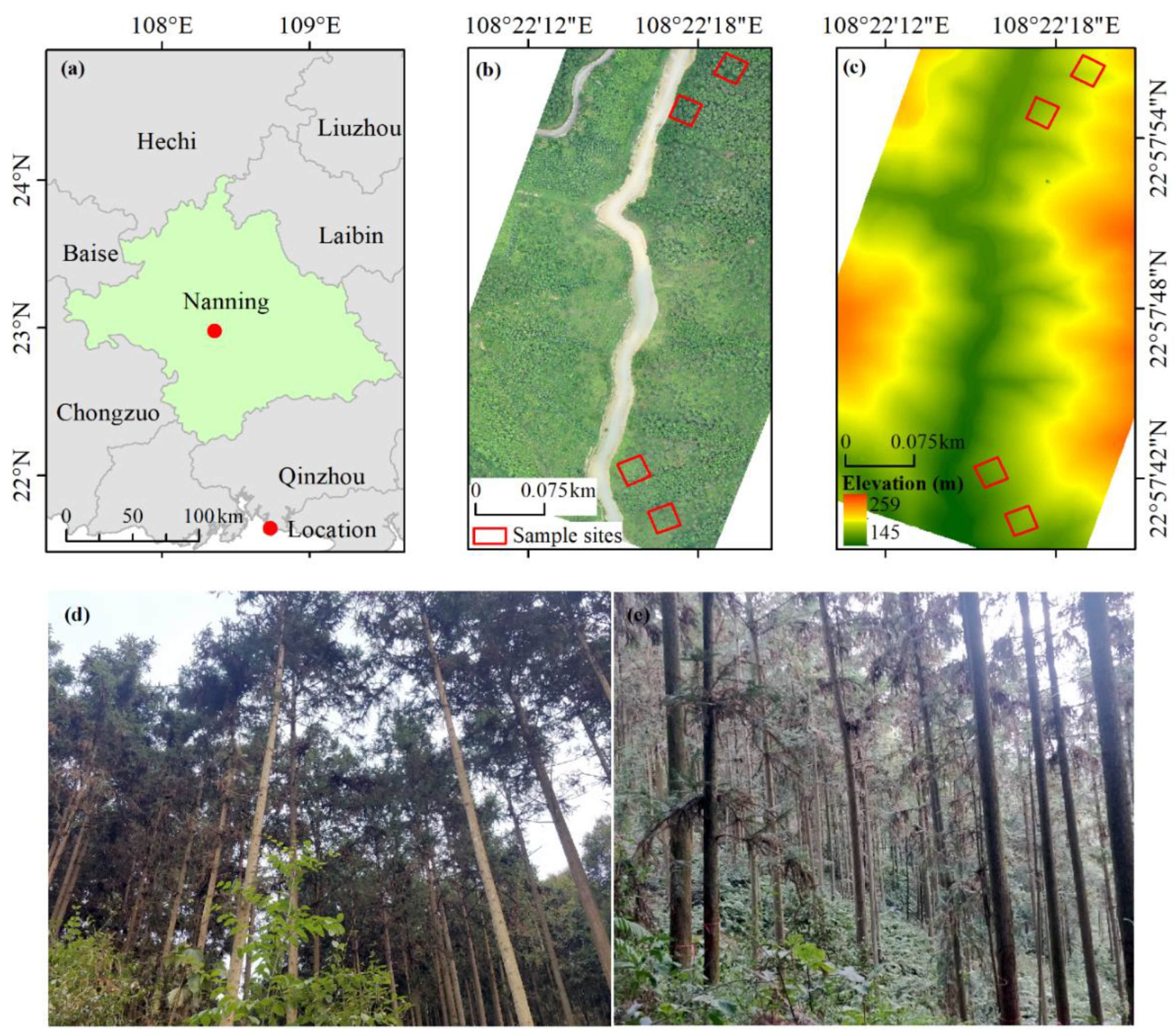
2.1. Study Area

The study area is located in Gaofeng forest farm in Guangxi province of southern China (108°20′57″–108°21′54″E, 22°57′08″–22°58′41″N) (Figure 1). The length in east-west and north-south direction of the region are is 2800 m and 1600 m respectively, with a total area of about 3.03 km². The forest farm belongs to subtropical monsoon climate, with sufficient sunshine and rainfall. The annual average temperature is 21.7 °C and the annual average precipitation is 1300 mm. The elevation varies from 125 m to 300 m. The forest type is mainly artificial forest with tall and dense trees, high canopy density and rich tree species. The dominant tree species include Chinese fir (Cunninghamia lanceolata (Lamb.) Hook.), eucalyptus (Eucalyptus robusta Smith), Castanopsis hystrix Miq. (Castanopsis hystrix J. D. Hooker et Thomson ex A. De Candolle). Among them, Chinese fir has ecological, economic and medicinal values. However, the complex terrain and high canopy density of the forest farm bring challenges to the estimation of IT-AGB.

Figure 1. Overview of the study area. (a) Location of study area; (b) Digital orthophoto model (DOM) and distribution of sample sites; (c) Digital elevation model (DEM). (d,e) are ground photographs of the sample plots and trees.

2.2. Data

2.2.1. Field Data

Field data collection was carried out from 5 to 14 January 2020, and the measured data of four Chinese fir sample plots (25 m × 25 m) (Figure 1) were obtained. We measured the diameter at breast height (DBH), tree height and crown width of individual trees in the sample plots, and recorded the slope, aspect, elevation, canopy density and other information of the sample plots. At the same time, we measured the position of individual tree in the sample plots using the Global Navigation Satellite System (GNSS) real-time kinematic (GNSS RTK) system, following the UTM projection (zone 49 N) with WGS-1984 Datum. We obtained a fix solution under each tree. The horizontal positioning accuracy is within ±0.2 m.

According to the measured tree height and DBH, the IT-AGB was calculated by using the allometric growth equation referring to “Comprehensive Database of Biomass Regressions for China’s Tree Species” [39], which was used as the true value of IT-AGB.

$$Y=71.2465\times {{\displaystyle ({{\displaystyle D}}^{2}H)}}^{0.9256}$$

(1)

where, Y is IT-AGB (kg); D is DBH (m); H is the tree height (m).

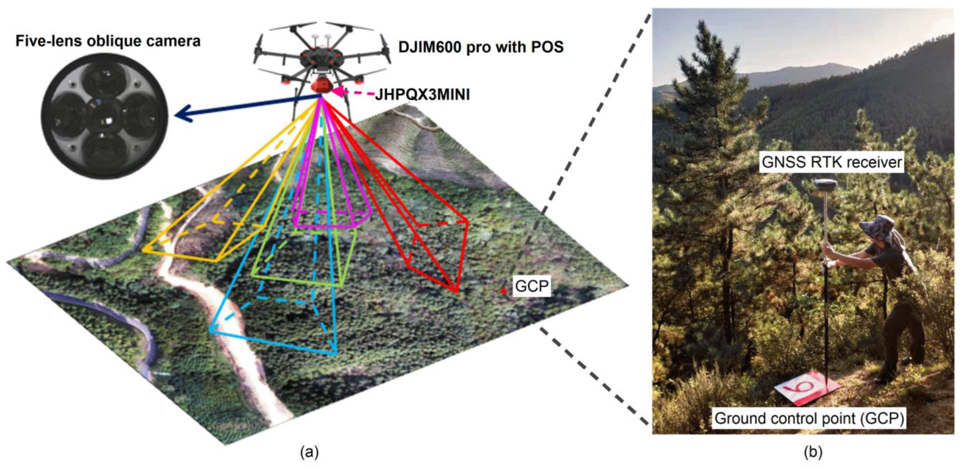
2.2.2. UAV Oblique Photography Data and Auxiliary Terrain Data

The image data were obtained at noon on 7 January 2020 using the DJIM600pro multi-rotor UAV equipped with JHPQX3MINI five-lens oblique camera (Figure 2) to acquire multi-angle photos. The camera parameters are shown in Table 1. Prior to flying, 10 ground control points (GCPs) were marked in the open area using 50 × 50 cm targets. The position of the GCPs is measured by GNSS RTK, and its horizontal and vertical accuracy is controlled within ±0.2 m for image data calibration processing.

Figure 2. Schematic diagram of data collection for (a) UAV equipped with five-lens oblique camera and (b) GCP.

Table 1. Flight and camera parameters of UAV oblique photogrammetry.

Sensors and Flight Parameters	JHP QX3MINI
Sensor size (mm × mm)	23.5 × 15.6
Heading overlap (%)	80
Side overlap (%)	70
Horizontal speed (m·s−1)	4~8
Flight altitude (m)	100
Exposure interval (s)	0.8~4.5
Focal length (mm)	35
Scanning angle (°)	45
Single camera pixel numbers (million)	42

In February 2018, we obtained LiDAR data using the RIEGL LMS-Q680i LiDAR sensor as auxiliary terrain data. The LiDAR sensor and flight parameters are shown in Table 2. LiDAR data processing mainly includes noise point removal and filtering. The noise point removal mainly removes the points within the abnormal elevation range. The ground points and non-ground points are separated by Cloth Simulation Filter (CSF) method, and then the ground points are interpolated by Triangulated Irregular Network (TIN) to generate Digital Terrain Model (DTM) with spatial resolution of 1 m, which is used to normalize the oblique photography point cloud data.

Table 2. LiDAR sensor and flight parameters.

Sensors and Flight Parameters	Parameter Values
Wavelength (nm)	1550
Beam divergence angle (mrad)	0.5
Spot diameter (cm)	45
Pulse repetition rate (kHz)	360
Pulse emission frequency (Hz)	112
Flight altitude (m)	900
Flight speed (m/s)	55

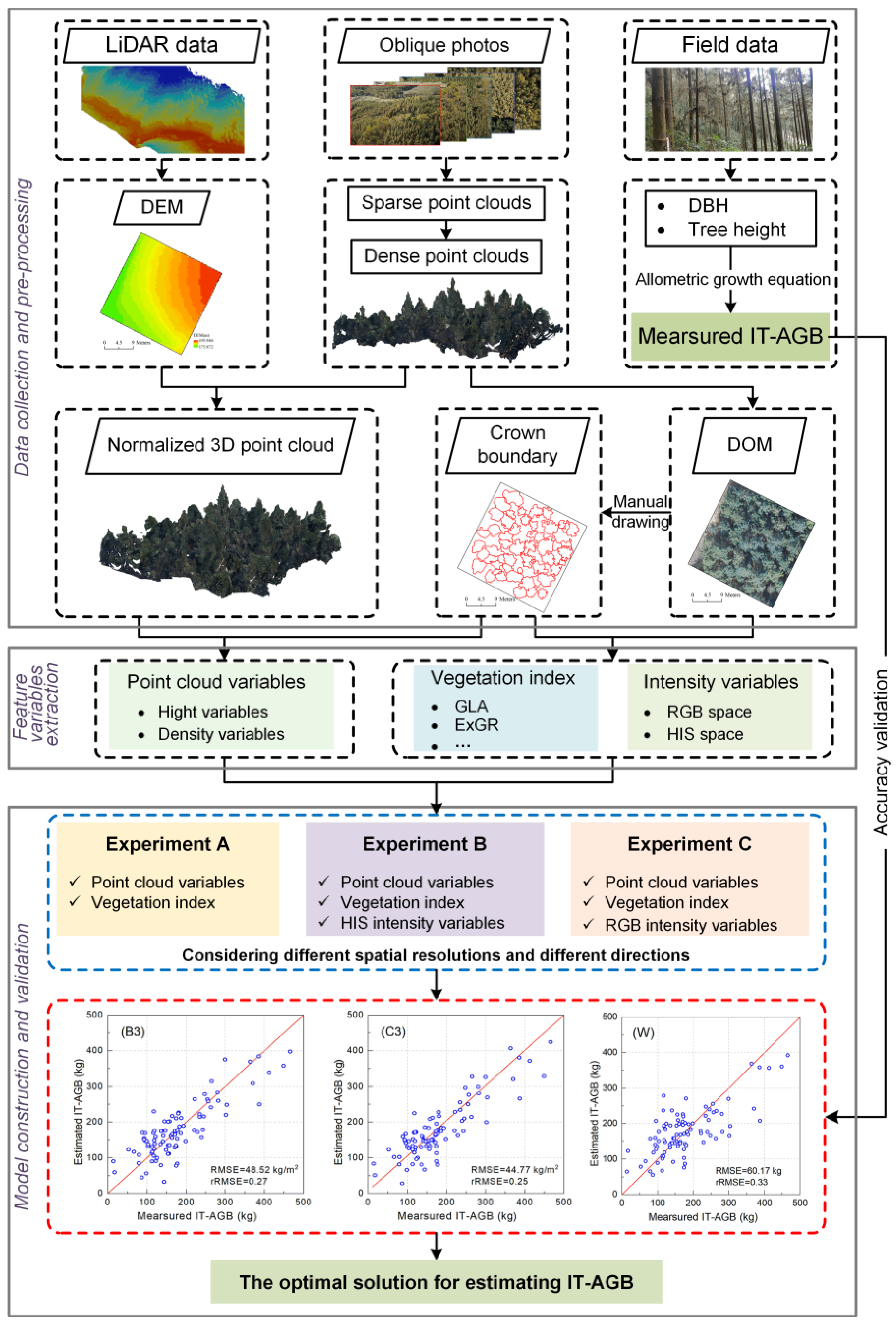
2.3. Data Processing

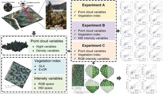
We used the CloudCompare (http://www.danielgm.net/cc/, accessed on 20 November 2021) [40].to generate dense point clouds through the incremental SfM [41] and Semi-Global Matching (SGM) algorithm. Because the oblique photogrammetry technology cannot obtain the terrain information under the forest when the canopy density is high [27,42]. The DTM data obtained from LiDAR data is used to normalize the dense point cloud to generate the normalized three-dimensional point cloud [28,36,43]. Moreover, radiation correction was performed on the point cloud spectrum data by dividing the DN of each band (red, green, and blue) by the sum of the DN values of all bands corresponding to the same 3D point [44,45]. TIN is used to generate Digital Orthophoto Model (DOM) with a resolution of 0.05 m.

2.4. Methods

The overall workflow is shown in Figure 3. The process consists of three steps: (1) the LiDAR data, UAV oblique photos and field data (DBH and tree height) of the sample plots were collected and preprocessed. (2) Based on point cloud data and DOM data obtained from UAV oblique photos, point cloud variables, vegetation index and intensity variables were extracted respectively. (3) Evaluating the effects of different color spatial intensity information, different spatial resolution and directions on the performance of the model.

Figure 3. Methodology Flowchart.

2.4.1. Individual Tree Segmentation

The main objective of this study is to explore the potential of oblique photography in IT-AGB estimation and the influence of spatial resolution on the estimation results. In order to avoid the influence of individual tree segmentation error on the accuracy of IT-AGB estimation, this study uses DOM data to draw the crown contour in the sample plots as the individual tree segmentation result data using the software of LiDAR 360 (Version 5.0, GreenValley International, Beijing, China) (https://www.lidar360.com/, accessed on 16 January 2022). Compared with the automatic individual tree segmentation by software, the tree crown segmented by this method is more accurate. More importantly, the cumulative error caused by inaccurate segmentation does not need to be considered in AGB estimation. There are many researches on individual tree segmentation methods based on point cloud data and CHM data [46,47,48,49,50,51,52], which can be used to segment trees when using our proposed model to estimate IT-AGB. However, since this is not the main content of this study, we avoid the process of selecting, comparing and verifying individual tree segmentation methods.

2.4.2. Feature Variables Extraction

The intensity variables were introduced as an important parameter and combined with three-dimensional point cloud variables and two-dimensional vegetation index to develop a model of IT-AGB. We explored the influence of intensity variables on modeling accuracy. The intensity value of three-dimensional color point cloud can be calculated based on the color channel values corresponding to R, G and B bands [42]:

$$\mathrm{Intensity}=0.2\times R+0.72\times G+0.07\times B$$

(2)

The point cloud height variables can reflect the vertical structure information of forest canopy, and the point cloud density variables can reflect the horizontal structure information of forest canopy. Therefore, the point cloud variables can highlight the forest vegetation information from a three-dimensional perspective, so as to effectively estimate the forest IT-AGB. The two-dimensional vegetation index can reflect the difference of vegetation growth to a certain extent, so it can be used as a direct feature variable for estimating the IT-AGB.

In addition, we also compared the intensity variables derived from HSI and RGB color space to determine the impact of two-color space intensity variables on forest IT-AGB estimation. Therefore, 10 intensity variables, 42 height variables, 10-point cloud density variables and 7 vegetation index variables were extracted in this study (Table 3).

Table 3. Feature variables and descriptions.

Type	Variable	Formula	Describe
RGB space	${{\displaystyle Max}}_i$	——	Maximum intensity
	${{\displaystyle Min}}_i$	——	Minimum intensity
	${{\displaystyle Mean}}_i$	——	Mean intensity
	${{\displaystyle sum}}_i$	${{\displaystyle sum}}_i={\displaystyle \sum _{i=1}^n(0.2\times {{\displaystyle R}}_i+0.72\times {{\displaystyle G}}_i+0.07\times {{\displaystyle B}}_i)}$	Total intensity
	${{\displaystyle sum}}_{sqrt\_i}$	${{\displaystyle sum}}_{sqrt\_i}=\sqrt{sumi}$	Square root of intensity value
HSI space	${{\displaystyle I}}_{MAX}$	——	Maximum intensity
	${{\displaystyle I}}_{MIN}$	——	Minimum intensity
	${{\displaystyle I}}_{MEAN}$	——	Mean intensity
	${{\displaystyle I}}_{SUM}$	——	Total intensity
	${{\displaystyle I}}_{SUM\_SQRT}$	——	Square root of intensity value
Hight variables	Haad	$Haad=\frac{{\displaystyle {\sum }_{i=1}^n(|Zi-\overline{Z}|)}}{n}$	Mean absolute deviation, $Z_i$ is the height of the ith point in each unit, $\overline{Z}$ is the average height of all points, n is the total number of points in each statistical unit.
	HAIQ	——	Cumulative height percentile interquartile spacing
	Hkurtosis	$H_{kurtosis}=\frac{\frac{1}{n}{\displaystyle {\sum }_{i=1}^n{{\displaystyle (Zi-\overline{Z})}}^4}}{{{\displaystyle (\frac{1}{n}{\displaystyle {\sum }_{i=1}^n{{\displaystyle (Zi-\overline{Z})}}^2)}}}^2}-3$	Height kurtosis
	Hcv	$Hcv=\frac{{{\displaystyle Z}}_{std}}{{{\displaystyle Z}}_{mean}}\times 100\%$	Variation coefficient of Z value of all points in a statistical unit, Zstd and Zmean are the standard deviation of the height values of all points and the average height of all points in each statistical unit.
	Hredio	$Hredio=\frac{Zmean-Z\min }{Z\max -Z\min }$	Canopy fluctuation rate, Zmin, Zmax, Zmean are the minimum height, maximum height and average height of all points in each statistical unit
	Hstddev	${{\displaystyle H}}_{stddev}=\sqrt{\frac{{\displaystyle {\sum }_{i=1}^n{{\displaystyle (Zi-\overline{Z})}}^2}}{n}}$	Standard deviation of Z values of all points in a statistical unit
	Hvariance	${{\displaystyle H}}_{\mathrm{var}iance}=\frac{{\displaystyle {\sum }_{i=1}^n{{\displaystyle (Zi-\overline{Z})}}^2}}{n}$	Variance of Z values of all points in a statistical unit
	Hskewness	${{\displaystyle H}}_{skewness}=\frac{\frac{1}{n}{\displaystyle {\sum }_{i=1}^n{{\displaystyle (Zi-\overline{Z})}}^3}}{{{\displaystyle (\frac{1}{n-1}{\displaystyle {\sum }_{i=1}^n{{\displaystyle (Zi-\overline{Z})}}^2)}}}^{\frac{3}{2}}}$	Height skewness
	H1…99th	——	1…99% cumulative height percentile
	Hmax, min, mean, median	——	The maximum, minimum, average and median of the point cloud after normalization
	P1st,…,99th	——	75%, 95% high percentile
density variables	D0,…,9	——	The proportion of height points greater than 30%, 50%, 70%, and 90% to all points
Vegetation index	CIVE	$CIVE=0.44R-0.88G+0.398+18.79$	Color index of vegetation [53]
	ExG	$ExG=2G-R-B$	Excess green index [54]
	ExGR	$ExGR=ExG-1.4R-G$	Excess green minus excess red index [55]
	GLA	$GLA=\frac{2\times G-R}{2\times G+R+B}$	Green leaf algorithm [56]
	NGRDI	$NGRDI=\frac{G-R}{G+R}$	Normalized green–red difference index [56]
	VEG	$VEG=\frac{G}{{{\displaystyle R}}^a{{\displaystyle B}}^{(1-a)}},a=0.67$	Vegetation index [57]
	COM	$\begin{array}{l}COM=0.25ExG+0.3ExGR\\ +0.33CIVE+0.12VEG\end{array}$	Combination index [58]

2.4.3. Construction of Empirical Model

The Pearson correlation analysis and stepwise regression method were used to screen the modeling features from 69 variables. In order to compare the contribution of different color spatial variables and the effects of different spatial resolutions to IT-AGB estimation, three kinds of feature variables combination experiments were designed based on five different spatial resolutions (0.05 m, 0.1 m, 0.2 m, 0.5 m and 1 m): point cloud variables + vegetation index (experiment A), point cloud variables + vegetation index + HSI intensity variables (experiment B) and point cloud variables + vegetation index + RGB intensity variables (experiment C). The different resolution image was obtained by nearest neighbor interpolation resampling methods.

In order to solve the point or block-like invalid data formed in the 3D reconstruction process that may be caused by factors such as tree canopy mutual occlusion and terrain (Figure 4). We proposed a method for estimating IT-AGB using only data from one direction (East, West, South, and North) of the canopy (Figure 5) when the obtained data is invalid or abnormal, and explored the feasibility of this method without greatly reducing the accuracy. The calculated IT-AGB from the allometric growth equation was used as the dependent variable, and the three-dimensional point cloud and the feature variables extracted from the point cloud data and RGB image data of the tree canopy in the corresponding direction were used as independent variables to establish estimation model.

Figure 4. Point-like or spot-like abnormal areas after 3D reconstruction. (a) is the DOM data of a sample plots. (b) is the DSM data of a sample plots and the red circle is the point or block-like invalid data.

Figure 5. Map of tree canopy division in different directions.

2.4.4. Accuracy Verification

We used the leave-one-out cross-validation approach to evaluate the model results and used the coefficient of determination (R²), root mean square error of leave-one-out cross-validation (RMSECV) and relative RMSECV (rRMSECV) to verify the predictive ability of the models.

$${{\displaystyle R}}^2=1-\frac{{\displaystyle \sum _{i=1}^n{{\displaystyle ({{\displaystyle Y}}_i-\overline{Y})}}^2}}{{\displaystyle \sum _{i=1}^n{{\displaystyle ({{\displaystyle Y}}_i^{\prime }-\overline{Y})}}^2}}$$

(3)

$$RMSECV=\sqrt{\frac{1}{n}{\displaystyle \sum _{i=1}^n{{\displaystyle ({{\displaystyle Y}}_i-{{\displaystyle Y}}_i^{\prime })}}^2}}$$

(4)

$$rRMSECV=\frac{RMSECV}{\overline{Y}}\times 100\%$$

(5)

where, $Y_i$ represents the predicted IT-AGB; $Y_i^{\prime }$ represents the measured IT-AGB; $\overline{Y}$ represents the measured average value of IT-AGB; n is the number of trees.

3. Results

3.1. IT-AGB Distribution of Sample Plots

The four sample plots of measured IT-AGB are shown in Table 4. In general, IT-AGB of the sample plots has a strong heterogeneity, ranging from 19.94 to 465.61 kg, and the standard deviation reaches 92.73 kg. Sample plot 1 has a complex tree age structure. The variation ranges of DBH and tree height are 10.10 cm~36.90 cm and 9.20 m~24.50 m, and the IT-AGB has broad distribution range. Most of the trees in sample plot 2 and plot 3 are mature trees, with an average DBH and average tree height of 21.72 cm and 25.75 cm, 20.16 m and 19.84 m respectively. The situation of sample plot 4 is similar to that of sample plot 1. The average IT-AGB is 153.89 kg and the standard deviation is 125.87 kg. The average IT-AGB of the four sample plots is more than 170 kg, which is prone to saturation by using optical images [59]. Therefore, we estimate the IT-AGB by using the oblique photography technology that can provide spectral, horizontal and vertical structural features.

Table 4. Statistical analysis of measured data of sample plots.

Sample Number	Number of Trees	Sample Characteristics	DBH (cm)	Tree Height (m)	AGB (kg)
1	51	Maximum	36.90	24.50	448.85
		minimum	10.10	9.20	21.85
		Mean	20.90	18.53	153.23
		Standard deviation	5.10	2.68	81.18
2	40	Maximum	31.50	23.60	376.41
		minimum	12.50	15.80	51.88
		Mean	21.72	20.16	175.35
		Standard deviation	5.11	2.12	84.21
3	28	Maximum	33.90	25.80	386.73
		minimum	18.00	14.10	98.07
		Mean	25.75	19.84	227.85
		Standard deviation	4.11	3.25	79.23
4	30	Maximum	34.80	26.10	465.611
		minimum	5.90	4.50	19.94
		Mean	18.55	14.19	153.89
		Standard deviation	8.59	6.11	125.87
Total	149	Maximum	36.90	26.10	465.61
		minimum	5.90	4.50	19.94
		Mean	21.53	19.39	170.51
		Standard deviation	6.04	3.97	92.73

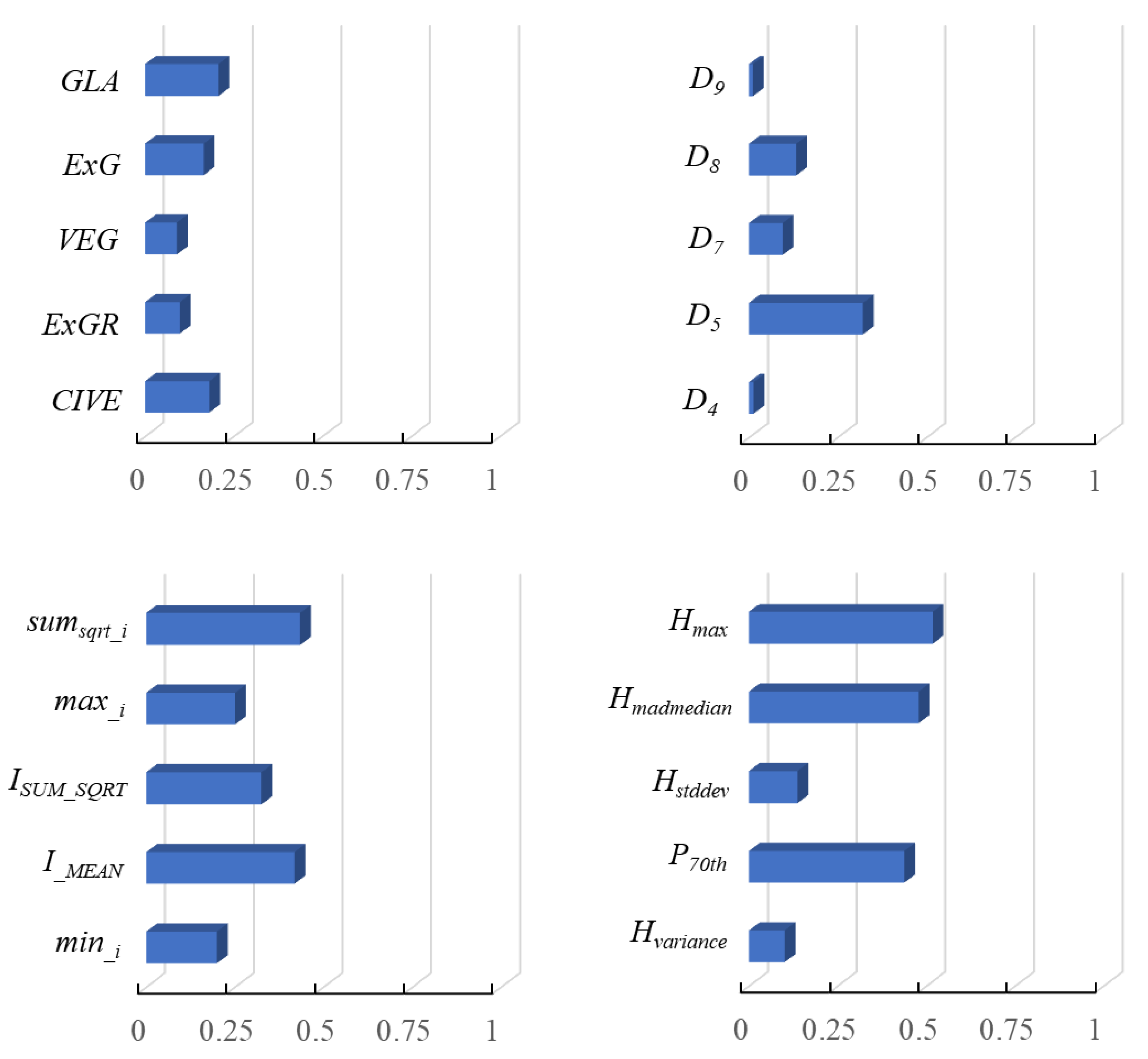
3.2. Features Selection

The correlation coefficients between 69 variables and IT-AGB were calculated by Pearson correlation analysis (Figure 6). The results showed that point cloud height variable had a high correlation with IT-AGB, while the two-dimensional vegetation index had a low correlation with IT-AGB. The top 20 variables (see Figure 6) with a high correlation coefficient were selected for modeling. The best variables combination for estimating forest IT-AGB was selected through stepwise regression analysis, including vegetation index GLA, point cloud density variables D₅, height variables H_max and H_30th, and intensity variables sum_{sqrt_i} and I_{SUM_SQRT}. GLA is the color vegetation index, which can be used to distinguish vegetation from non-vegetation. Point cloud height variables reflects forest vertical structure information. Point cloud density variables is highly sensitive to forest AGB, and reflects forest horizontal structure information. The intensity value calculated based on RGB and HSI color space has strong correlation with IT-AGB (Figure 6).

Figure 6. Variable correlations with IT-AGB (Top 20 variables).

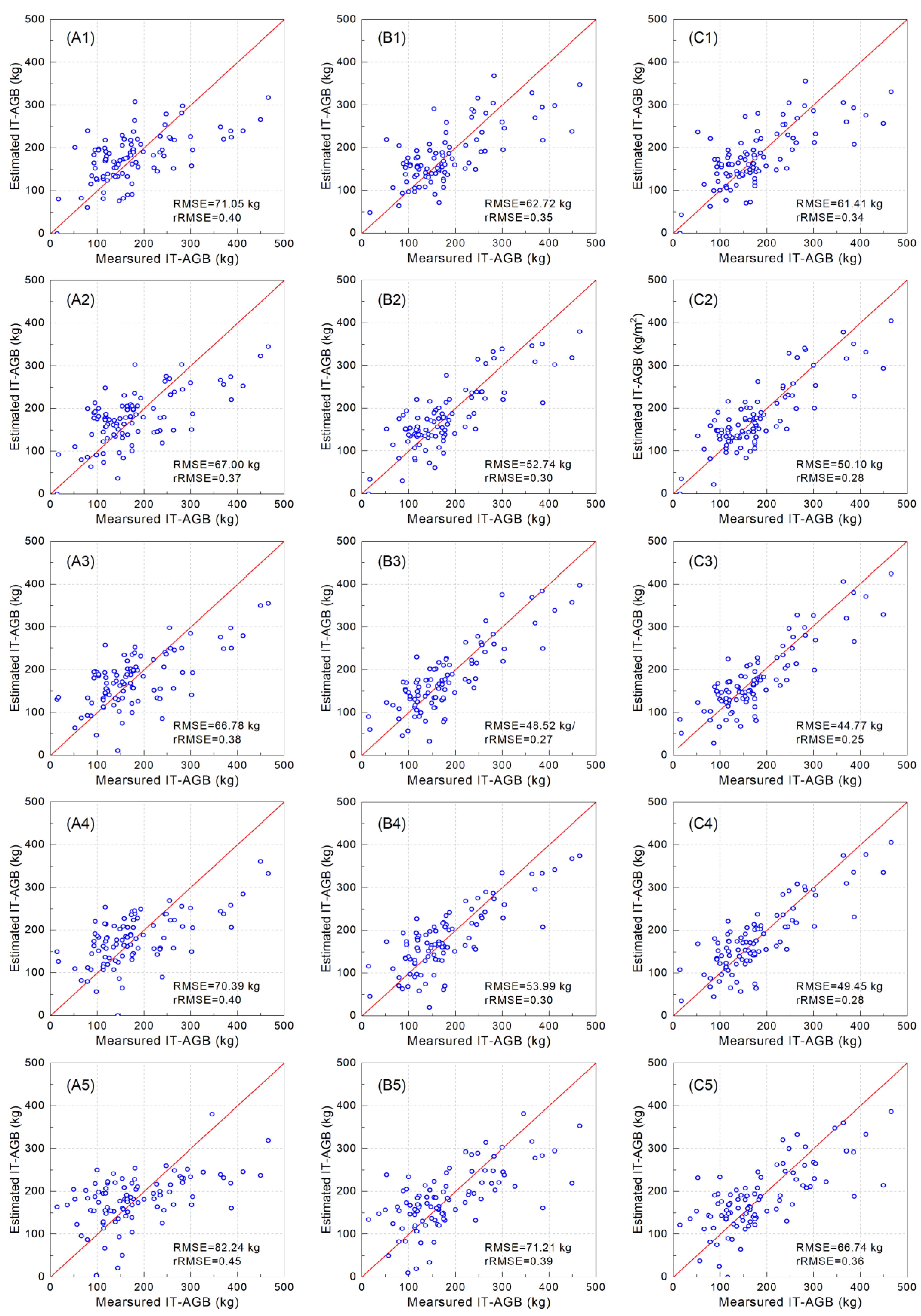
3.3. Contribution of Different Intensity Information and Spatial Resolution on Model

The selected variables were used to develop IT-AGB estimation model by multiple linear regression (Table 5). It can be seen from Table 5 that the AGB estimation models constructed with different types and spatial resolution of variables varied considerably. The variation ranges of R² and RMSECV were 0.34~0.79 and 44.77~82.24 kg respectively, and rRMSECV was 0.25~0.45. The estimation accuracy of the model was the best at a spatial resolution of 0.2 m, which was significantly improved compared with the spatial resolution of the other four. However, when the spatial resolution was increased from 1 m to 0.5 m, both the value of RMSECV or rRMSECV were similar or same, which meant that the model accuracy was not significantly improved.

Table 5. Accuracy evaluation of models with different spatial resolution and variables.

Model		Model Equation	R2	RMSECV (kg)	rRMSECV
0.05 m	A	$\begin{array}{l}Y=-508.187+241.946\times GLA+2535.144\times {{\displaystyle D}}_5\\ -24.819\times {{\displaystyle H}}_{30\mathrm{th}}+51.368\times {{\displaystyle H}}_{\max }\end{array}$	0.44	71.05	0.40
	B	$\begin{array}{l}Y=-561.402+720.154\times GLA+2335.538\times {{\displaystyle D}}_5\\ -24.972\times {{\displaystyle H}}_{30\mathrm{th}}+51.822\times {{\displaystyle H}}_{\max }+0.090\times {{\displaystyle I}}_{SUM\_SQRT}\end{array}$	0.57	62.72	0.35
	C	$\begin{array}{l}Y=-505.267+404.231\times GLA+2057.729\times {{\displaystyle D}}_5\\ -21.371\times {{\displaystyle H}}_{30\mathrm{th}}+47.405\times {{\displaystyle H}}_{\max }+0.088\times {{\displaystyle sum}}_{sqrt\_i}\end{array}$	0.59	61.41	0.34
0.1 m	A	$\begin{array}{l}Y=-454.307+600.580\times GLA+2497.540\times {{\displaystyle D}}_5\\ -48.036\times {{\displaystyle H}}_{30\mathrm{th}}+70.815\times {{\displaystyle H}}_{\max }\end{array}$	0.49	67.00	0.37
	B	$\begin{array}{l}Y=-592.935+1219.055\times GLA+2700.810\times {{\displaystyle D}}_5\\ -50.306\times {{\displaystyle H}}_{30\mathrm{th}}+75.790\times {{\displaystyle H}}_{\max }+0.111\times {{\displaystyle I}}_{SUM\_SQRT}\end{array}$	0.70 **	52.74	0.30
	C	$\begin{array}{l}Y=-556.908+819.871\times GLA+2579.594\times {{\displaystyle D}}_5\\ -44.905\times {{\displaystyle H}}_{30\mathrm{th}}+70.367\times {{\displaystyle H}}_{\max }+0.109\times {{\displaystyle sum}}_{sqrt\_i}\end{array}$	0.72 **	50.10	0.28
0.2 m	A	$\begin{array}{l}Y=-350.353+1081.184\times GLA+1891.010\times {{\displaystyle D}}_5\\ -49.732\times {{\displaystyle H}}_{30\mathrm{th}}+67.582\times {{\displaystyle H}}_{\max }\end{array}$	0.50	66.78	0.38
	B	$\begin{array}{l}Y=-529.350+1809.895\times GLA+1919.730\times {{\displaystyle D}}_5\\ -48.844\times {{\displaystyle H}}_{30\mathrm{th}}+72.289\times {{\displaystyle H}}_{\max }+0.125\times {{\displaystyle I}}_{SUM\_SQRT}\end{array}$	0.75 **	48.52	0.27
	C	$\begin{array}{l}Y=-503.178+1314.658\times GLA+1695.792\times {{\displaystyle D}}_5\\ -40.214\times {{\displaystyle H}}_{30\mathrm{th}}+65.158\times {{\displaystyle H}}_{\max }+0.125\times {{\displaystyle sum}}_{sqrt\_i}\end{array}$	0.79 **	44.77	0.25
0.5 m	A	$\begin{array}{l}Y=-326.319+1048.792\times GLA+770.335\times {{\displaystyle D}}_5\\ -35.794\times {{\displaystyle H}}_{30\mathrm{th}}+55.757\times {{\displaystyle H}}_{\max }\end{array}$	0.44	70.39	0.40
	B	$\begin{array}{l}Y=-512.761+1761.952\times GLA+755.589\times {{\displaystyle D}}_5\\ -33.174\times {{\displaystyle H}}_{30\mathrm{th}}+59.510\times {{\displaystyle H}}_{\max }+0.124\times {{\displaystyle I}}_{SUM\_SQRT}\end{array}$	0.69 **	53.99	0.30
	C	$\begin{array}{l}Y=-498.311+1279.555\times GLA+1678.740\times {{\displaystyle D}}_5\\ -25.901\times {{\displaystyle H}}_{30\mathrm{th}}+53.839\times {{\displaystyle H}}_{\max }+0.128\times {{\displaystyle sum}}_{sqrt\_i}\end{array}$	0.74 **	49.45	0.28
1 m	A	$\begin{array}{l}Y=-273.155+553.142\times GLA+184.608\times {{\displaystyle D}}_5\\ -17.770\times {{\displaystyle H}}_{30\mathrm{th}}+39.409\times {{\displaystyle H}}_{\max }\end{array}$	0.34	82.24	0.45
	B	$\begin{array}{l}Y=-441.875+1227.558\times GLA+211.609\times {{\displaystyle D}}_5\\ -13.633\times {{\displaystyle H}}_{30\mathrm{th}}+40.918\times {{\displaystyle H}}_{\max }+0.114\times {{\displaystyle I}}_{SUM\_SQRT}\end{array}$	0.52	71.21	0.39
	C	$\begin{array}{l}Y=-439.854+829.448\times GLA+201.563\times {{\displaystyle D}}_5\\ -7.326\times {{\displaystyle H}}_{30\mathrm{th}}+36.344\times {{\displaystyle H}}_{\max }+0.124\times {{\displaystyle sum}}_{sqrt\_i}\end{array}$	0.58	66.74	0.36

Note: ** indicates p < 0.001.

The estimation accuracy of IT-AGB was significantly improved by introducing intensity variables combined with vegetation index and point cloud variables (Table 5). Among them, the models of experiment C have the highest R² (0.59, 0.72, 0.79, 0.74 and 0.58) and the lowest RMSECV (61.41, 50.10, 44.77, 49.45 and 66.74 kg) at corresponding resolutions (0.05, 0.1, 0.2, 0.5 and 1 m). Taking the spatial resolution of 0.2 m as an example, compared with the intensity variable of RGB space, the contribution of HSI space variable to the estimation model was slightly lower, with R² of 0.75 and RMSECV of 48.52 kg. The R² of the experiment A models was low, only 0.50. Overall, the IT-AGB estimation model of experiment C was more stable and robust.

The scatterplots of the predicted and measured IT-AGB are shown in Figure 7. When the spatial resolution was 0.2 m, the estimation model of experiment C was the best (Figure 7C3), which scatter points were evenly distributed on both sides of y = x, indicating that the introduction of RGB spatial information can improve the estimation accuracy. When the spatial resolution was 0.05 m and 1 m, the scatter distribution was scattered, and the performance of the model was poor. Compared with the model of experiment A (Figure 7A3), the estimation accuracy of the experiment B (Figure 7B3) and experiment C (Figure 7C3) models were improved by 11% and 13% respectively, when the spatial resolution was 0.2 m.

Figure 7. Scatterplots of measured and predicted IT-AGB. Ai, Bi and Ci are models with spatial resolutions of 0.05 m, 0.1 m, 0.2 m, 0.5 m and 1 m, respectively; (A1–A5) are models of experiment A; (B1–B5) are models of experiment B; (C1–C5) are models of experiment C. The red line in the figure is the line of y = x.

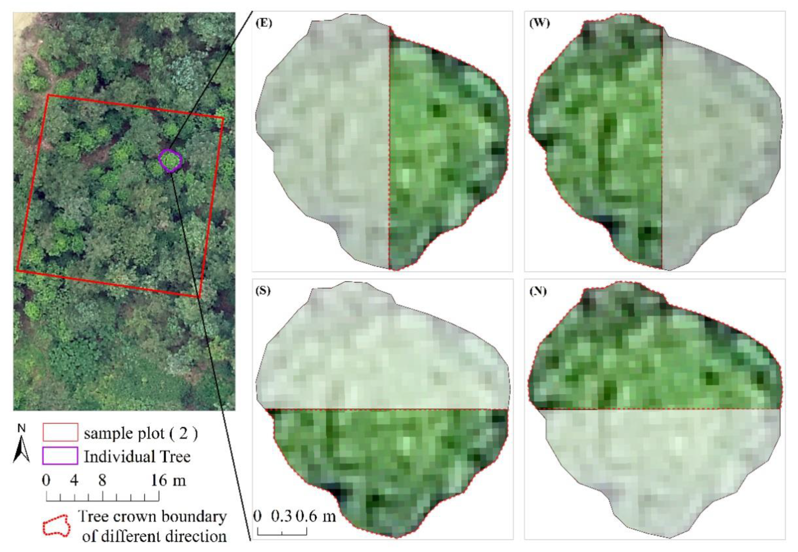
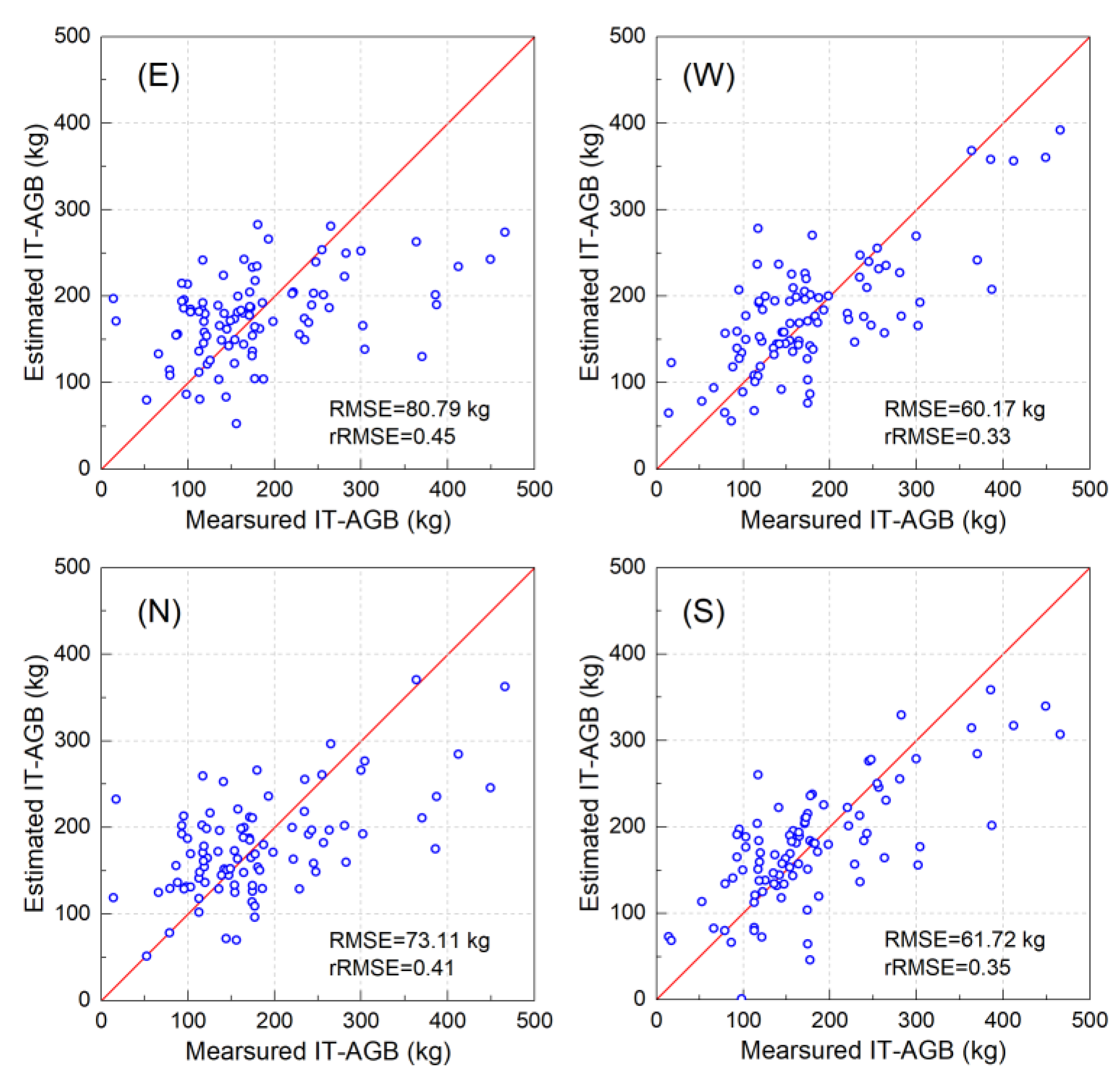
3.4. Comparisons of Models in Different Tree Canopy Directions

There are obvious accuracy differences in the IT-AGB models in different individual canopy horizontal directions (Table 6). The R² and rRMSECV of the estimation models in different directions ranged from 0.29~0.60 and 0.33~0.45 respectively. The results showed that the performance of West-model was greater than that of South-model, North-model and East-model, and the estimation accuracy was improved by 2%, 8% and 12% respectively. The West-model can best reflect the overall IT-AGB with R² reaching 0.60 and RMSECV of 60.17 kg. The second was the South-model with R² of 0.58 and rRMSECV of 0.35. The East-model was the worst with R² of only 0.29 and RMSECV of 80.79 kg.

Table 6. Accuracy evaluation of models in different directions.

Model	Model Equation	R2	RMSECV (kg)	rRMSECV
East	$\begin{array}{l}Y=-186.079+884.733\times GLA+1346.804\times D5\\ +38.489\times H_{\max }-29.545\times H_{30\mathrm{th}}+0.116\times su{m}_{sqrt\_i}\end{array}$	0.29	80.79	0.45
North	$\begin{array}{l}Y=-373.301+880.425\times GLA+1898.861\times D5\\ +47.219\times H_{\max }-34.777\times H_{30\mathrm{th}}+0.271\times su{m}_{sqrt\_i}\end{array}$	0.42	73.11	0.41
South	$\begin{array}{l}Y=-365.544+712.880\times GLA+1217.608\times D_5\\ +51.278\times H_{\max }-30.879\times H_{30\mathrm{th}}+0.109\times su{m}_{sqrt\_i}\end{array}$	0.58 **	61.72	0.35
West	$\begin{array}{l}Y=-468.532+724.398\times GLA+1875.551\times D5\\ +56.608\times H_{\max }-35.762\times H_{30\mathrm{th}}+0.183\times su{m}_{sqrt\_i}\end{array}$	0.60 **	60.17	0.33

Note: ** indicates p < 0.001.

Scatterplots of predicted and measured IT-AGB in different horizontal directions are shown in Figure 8. The estimation ability of models varies greatly in different directions, and only the West-model met the estimation requirements; the scattered points were uniformly distributed on both sides of y = x, the RMSECV was the lowest (60.17 kg), and the rRMSECV was only 0.33. The East-model has the worst estimation accuracy, with different degrees of underestimation and overestimation.

Figure 8. Scatterplots of measured and predicted IT-AGB in different direction.

4. Discussion

4.1. Extraction of Feature Variables for Modeling

Feature variables, include GLA, D₅, H_max, H_30th, sum_{sqrt_i} and I_{SUM_SQRT} were selected as the final modeling variables by Pearson correlation analysis and stepwise regression. The Chinese fir has lanceolate or strip lanceolate leaves, conical crown and concentrated crown distribution. The point cloud density can digitize the above features and better highlight the forest horizontal structure crown information. The H_max and H_30th are point cloud height variables that reflect the information of height related to the forest AGB and the vertical structure of the forest crown [25,60,61]. The GLA can effectively distinguish vegetation from other features, and is a good correlation between vegetation index and AGB [38,41]. Furthermore, the sum_{sqrt_i} (intensity variable of the RGB spatial) [42] and I_{SUM_SQRT} (intensity variable of HSI spatial) can reflect image features and the spatial information contained in the image. The relatively compact canopy structure rarely allows ground information to pass through, so there are fewer mutations in intensity information. This makes the description of the forest canopy surface information more accurate, which can explain the usefulness of the intensity information to IT-AGB. In brief, the combination of horizontal and vertical structure information with RGB or HSI spatial intensity variables can reflect the IT-AGB information more comprehensively.

4.2. Effects of Different Spatial Resolution on Models

In this study, we used five different resolution images (0.05 m, 0.1 m, 0.2 m, 0.5 m and 1 m) to extract feature variables and construct IT-AGB estimation models. With the increase of spatial resolution, the model effect showed a trend of first increasing and then decreasing. Compared with the image resolution 0.5 m, the resolution image 0.1 m and 0.05 m did not significantly improve the estimation accuracy, and the 0.2 m resolution estimation model was significantly better than the other four. The image with low spatial resolution is greatly disturbed by the mixed pixel effect, which affects the accuracy of estimation [62,63]. Theoretically, with the improvement of spatial resolution, the effects of mixed pixels on extracted variables decreases, and the model accuracy also gets improved. However, the result of our research was inconsistent with this law. The reason may be that we used the DEM provided by LiDAR data to normalize the point cloud data obtained from oblique photos. The density of LiDAR point cloud is low, and the 1 m spatial resolution DEM generated by interpolation method is different from real terrain, especially in areas with large slope, which will affect the processing of normalized point cloud. Here, we take a tree as an example to explain. In the Figure 9, an individual tree canopy covered about 20 pixels (1 m × 1 m) of DEM data. The point cloud of the individual tree subtracted the elevation value of the corresponding pixel to complete the point cloud normalization process, and then the height variable was extracted. With the increase of the resolution of the extracted point cloud variables, the influence of the point cloud normalized by DEM (1 m spatial resolution) on the height variables is more obvious. Therefore, the model effect decreases with the increase of spatial resolution when the spatial resolution is less than 0.2 m. The normalized point cloud will be infinitely closer to the individual tree condition in the real environment with the increasing spatial resolution of DEM, which is an ideal state. In addition, environmental conditions (such as slope, irradiance) and inter tree competition may also cause the scatter diagram of experiment C to be scattered (see Figure 6C1, C2, C4 and C5). In general, the best model we established has a certain applicability and stability (Figure 6C3). In the further study, we will deeply explore the impact of topographic and ecological factors on IT-AGB.

Figure 9. Schematic diagram of normalization of individual tree point cloud. (The short lines of different colors at the bottom of the left figure represent different DEM values, and the length is the pixel size of the corresponding DEM. The right figure is the top view of the left figure, each solid line grid is 1 m, and different colors represent different DEM values).

4.3. Effects of Intensity Information on Model

RGB space and HSI space are different representations of the same physical quantity. The description of intensity variables in RGB space can highlight vegetation information and is suitable for IT-AGB estimation. The main reason is that HSI color space conforms to human visual characteristics and is described by double cone space [64]. The intensity is expressed by the height by the axis direction in HSI space. The axis of the cone describes the gray level. The minimum and maximum intensity are black and white respectively. HSI color space is not related to color information, which only can simplify the workload of data processing. The RGB space is described by the cube space, and the description of intensity is a linear combination of the three color directions [65], which explains why the model containing RGB space-intensity information performs better.

4.4. Effects of Different Direction on Model

We compared the models in four horizontal directions of individual tree crowns, and the accuracy of the models was quite different. The West-model had the best performance, and the East-model had the worst performance (Table 6). The reason can be attributed to the effects of canopy structure, latitude, altitude and slope direction. Firstly, the canopy of Chinese fir is conical, and the canopy structure is relatively compact, which makes it difficult to penetrate for solar radiation. At the same time, the south and west of the canopy with high sunshine hours have strong vegetation photosynthesis in this study area, and the canopy structure is significantly different from the other directions, which can better express the information of the whole canopy. Finally, the growth status of trees in the Figure 10 show that the T₁ and T₂ (or T₃) compete for conditions such as space and sunlight in the growth process. Among them, the competition between T₁ and T₃ was essentially a competition between the westward canopy of T₁ and the eastward canopy of T₃, and the obvious advantage of T₁ was mainly manifested in the relatively high altitude. Similarly, the relationship between T₁ and T₂ was the competition between the northward crown of T₁ and the southward crown of T₂, which was a competition of equal status. This can also explain that the West-model performs better than that of South-model in the canopy of T₁. This could also explain the superior performance of the West-model in the T₁ canopy compared to the South-model.

Figure 10. Schematic diagram of sample plot forest competition.

In addition, we assumed that the canopy was divided into four pieces: A, B, C and D, where A + B, B + C, C + D and D + A were equivalent to the canopy of the west, south, east and north respectively and Model (A + B) > Model (C + B) through the Figure 10. It can be understood that the contribution of the direction of A was greater than that of the C, which makes it easy to understand that the East-model performs poorly compared to the North-model.

Therefore, we can infer the best direction for estimating the IT-AGB of the damaged data based on environmental factors such as terrain and slope, so as to obtain accurate IT-AGB information. Our method does not specifically limit the environment, and is suitable for most of the IT-AGB estimation with invalid data and other problems. However, if the quality of the obtained data was very unsatisfactory, such as more than 50% of the area in the individual tree crown cannot be identified, we recommend looking for the problem, resetting the conditions of flight and obtaining data.

5. Conclusions

We proposed a novel approach to estimating IT-AGB by combining the three-dimensional point cloud features, vegetation index and intensity information obtained by oblique photogrammetry technology, explored the impact of different color spatial intensity variables and spatial resolution on estimation model, and evaluated the ability of four directional data in individual tree crown to estimating IT-AGB. The introduction of intensity variables into the model improved the accuracy, and the contribution of RGB spatial information to the model was greater than that of HSI spatial information. Spatial resolution also affected estimation model, and the accuracy reached 75% when the spatial resolution was 0.2 m, which provided a scientific basis for the design of flying height. The West-model performed best, with an estimation accuracy of 67%, which can solve the problem of the IT-AGB estimation when the image quality was affected by uncontrollable factors. In short, we explored the potential of the combination of point cloud variables, vegetation index and intensity variables to estimate the IT-AGB of Chinese fir forest, with an accuracy of 75%. That is, using multi-dimensional features derived from oblique photogrammetry photos can realize the rapid and non-destructive estimation of IT-AGB in complex stand structure and environment, which provides support for the accurate investigation of forest resources and the accurate measurement of carbon stock.

References

- Gómez, C.; White, J.C.; Wulder, M.A.; Alejandro, P. Historical forest biomass dynamics modelled with Landsat spectral trajectories. ISPRS J. Photogramm. Remote Sens. 2014, 93, 14–28. [Google Scholar] [CrossRef] [Green Version]
- Zhu, X.; Liu, D. Improving forest aboveground biomass estimation using seasonal Landsat NDVI time-series. ISPRS J. Photogramm. Remote Sens. 2015, 102, 222–231. [Google Scholar] [CrossRef]
- Li, L.; Guo, Q.; Tao, S.; Kelly, M.; Xu, G. Lidar with multi-temporal MODIS provide a means to upscale predictions of forest biomass. ISPRS J. Photogramm. Remote Sens. 2015, 102, 198–208. [Google Scholar] [CrossRef]
- Luo, S.; Wang, C.; Xi, X.; Nie, S.; Fan, X.; Chen, H.; Ma, D.; Liu, J.; Zou, J.; Lin, Y.; et al. Estimating forest aboveground biomass using small-footprint full-waveform airborne LiDAR data. Int. J. Appl. Earth Obs. Geoinf. 2019, 83, 101922. [Google Scholar] [CrossRef]
- Malhi, R.K.M.; Anand, A.; Srivastava, P.K.; Chaudhary, S.K.; Pandey, M.K.; Behera, M.D.; Kumar, A.; Singh, P.; Sandhya Kiran, G. Synergistic evaluation of Sentinel 1 and 2 for biomass estimation in a tropical forest of India. Adv. Space Res. 2021, in press. [Google Scholar] [CrossRef]
- Campbell, M.J.; Dennison, P.E.; Kerr, K.L.; Brewer, S.C.; Anderegg, W.R.L. Scaled biomass estimation in woodland ecosystems: Testing the individual and combined capacities of satellite multispectral and lidar data. Remote Sens. Environ. 2021, 262, 112511. [Google Scholar] [CrossRef]
- Wang, G.; Zhang, M.; Gertner, G.Z.; Oyana, T.; McRoberts, R.E.; Ge, H. Uncertainties of mapping aboveground forest carbon due to plot locations using national forest inventory plot and remotely sensed data. Scand. J. For. Res. 2011, 26, 360–373. [Google Scholar] [CrossRef]
- Wang, Y.; Ni, W.; Sun, G.; Chi, H.; Zhang, Z.; Guo, Z. Slope-adaptive waveform metrics of large footprint lidar for estimation of forest aboveground biomass. Remote Sens. Environ. 2019, 224, 386–400. [Google Scholar] [CrossRef]
- Wang, Y.; Zhang, X.; Guo, Z. Estimation of tree height and aboveground biomass of coniferous forests in North China using stereo ZY-3, multispectral Sentinel-2, and DEM data. Ecol. Indic. 2021, 126, 107645. [Google Scholar] [CrossRef]
- Liao, Z.; He, B.; Quan, X.; van Dijk, A.I.J.M.; Qiu, S.; Yin, C. Biomass estimation in dense tropical forest using multiple information from single-baseline P-band PolInSAR data. Remote Sens. Environ. 2019, 221, 489–507. [Google Scholar] [CrossRef]
- Ploton, P.; Barbier, N.; Couteron, P.; Antin, C.M.; Ayyappan, N.; Balachandran, N.; Barathan, N.; Bastin, J.F.; Chuyong, G.; Dauby, G.; et al. Toward a general tropical forest biomass prediction model from very high resolution optical satellite images. Remote Sens. Environ. 2017, 200, 140–153. [Google Scholar] [CrossRef]
- Askne, J.I.H.; Soja, M.J.; Ulander, L.M.H. Biomass estimation in a boreal forest from TanDEM-X data, lidar DTM, and the interferometric water cloud model. Remote Sens. Environ. 2017, 196, 265–278. [Google Scholar] [CrossRef]
- Yang, H.; Li, F.; Wang, W.; Yu, K. Estimating Above-Ground Biomass of Potato Using Random Forest and Optimized Hyperspectral Indices. Remote Sens. 2021, 13, 2339. [Google Scholar] [CrossRef]
- Proisy, C.; Couteron, P.; Fromard, F.O. Predicting and mapping mangrove biomass from canopy grain analysis using Fourier-based textural ordination (FOTO) of IKONOS images. Remote Sens. Environ. 2007, 109, 379–392. [Google Scholar] [CrossRef]
- Yadav, S.; Padalia, H.; Sinha, S.K.; Srinet, R.; Chauhan, P. Above-ground biomass estimation of Indian tropical forests using X band Pol-InSAR and Random Forest. Remote Sens. Appl. Soc. Environ. 2021, 21, 100462. [Google Scholar] [CrossRef]
- Li, G.; Xie, Z.; Jiang, X.; Lu, D.; Chen, E. Integration of ZiYuan-3 Multispectral and Stereo Data for Modeling Aboveground Biomass of Larch Plantations in North China. Remote Sens. 2019, 11, 2328. [Google Scholar] [CrossRef] [Green Version]
- Zhao, P.; Lu, D.; Wang, G.; Wu, C.; Huang, Y.; Yu, S. Examining Spectral Reflectance Saturation in Landsat Imagery and Corresponding Solutions to Improve Forest Aboveground Biomass Estimation. Remote Sens. 2016, 8, 469. [Google Scholar] [CrossRef] [Green Version]
- Hu, T.; Zhang, Y.; Su, Y.; Zheng, Y.; Lin, G.; Guo, Q. Mapping the Global Mangrove Forest Aboveground Biomass Using Multisource Remote Sensing Data. Remote Sens. 2020, 12, 1690. [Google Scholar] [CrossRef]
- Cao, L.; Coops, N.C.; Innes, J.L.; Sheppard, S.R.J.; Fu, L.; Ruan, H.; She, G. Estimation of forest biomass dynamics in subtropical forests using multi-temporal airborne LiDAR data. Remote Sens. Environ. 2016, 178, 158–171. [Google Scholar] [CrossRef]
- Bazezew, M.N.; Hussin, Y.A.; Kloosterman, E.H. Integrating Airborne LiDAR and Terrestrial Laser Scanner forest parameters for accurate above-ground biomass/carbon estimation in Ayer Hitam tropical forest, Malaysia. Int. J. Appl. Earth Obs. Geoinf. 2018, 73, 638–652. [Google Scholar] [CrossRef]
- Duncanson, L.I.; Dubayah, R.O.; Cook, B.D.; Rosette, J.; Parker, G. The importance of spatial detail: Assessing the utility of individual crown information and scaling approaches for lidar-based biomass density estimation. Remote Sens. Environ. 2015, 168, 102–112. [Google Scholar] [CrossRef]
- Lu, J.; Wang, H.; Qin, S.; Cao, L.; Pu, R.; Li, G.; Sun, J. Estimation of aboveground biomass of Robinia pseudoacacia forest in the Yellow River Delta based on UAV and Backpack LiDAR point clouds. Int. J. Appl. Earth Obs. Geoinf. 2020, 86, 102014. [Google Scholar] [CrossRef]
- Nord-Larsen, T.; Schumacher, J. Estimation of forest resources from a country wide laser scanning survey and national forest inventory data. Remote Sens. Environ. 2012, 119, 148–157. [Google Scholar] [CrossRef]
- Eitel, J.U.H.; Höfle, B.; Vierling, L.A.; Abellán, A.; Asner, G.P.; Deems, J.S.; Glennie, C.L.; Joerg, P.C.; LeWinter, A.L.; Magney, T.S.; et al. Beyond 3-D: The new spectrum of lidar applications for earth and ecological sciences. Remote Sens. Environ. 2016, 186, 372–392. [Google Scholar] [CrossRef] [Green Version]
- Su, Y.; Guo, Q.; Xue, B.; Hu, T.; Alvarez, O.; Tao, S.; Fang, J. Spatial distribution of forest aboveground biomass in China: Estimation through combination of spaceborne lidar, optical imagery, and forest inventory data. Remote Sens. Environ. 2016, 173, 187–199. [Google Scholar] [CrossRef] [Green Version]
- Liu, K.; Shen, X.; Cao, L.; Wang, G.; Cao, F. Estimating forest structural attributes using UAV-LiDAR data in Ginkgo plantations. ISPRS J. Photogramm. Remote Sens. 2018, 146, 465–482. [Google Scholar] [CrossRef]
- Jayathunga, S.; Owari, T.; Tsuyuki, S. The use of fixed–wing UAV photogrammetry with LiDAR DTM to estimate merchantable volume and carbon stock in living biomass over a mixed conifer–broadleaf forest. Int. J. Appl. Earth Obs. Geoinf. 2018, 73, 767–777. [Google Scholar] [CrossRef]
- Li, B.; Xu, X.; Zhang, L.; Han, J.; Bian, C.; Li, G.; Liu, J.; Jin, L. Above-ground biomass estimation and yield prediction in potato by using UAV-based RGB and hyperspectral imaging. ISPRS J. Photogramm. Remote Sens. 2020, 162, 161–172. [Google Scholar] [CrossRef]
- Fu, X.; Zhang, Z.; Cao, L.; Coops, N.C.; Goodbody, T.R.H.; Liu, H.; Shen, X.; Wu, X. Assessment of approaches for monitoring forest structure dynamics using bi-temporal digital aerial photogrammetry point clouds. Remote Sens. Environ. 2021, 255, 112300. [Google Scholar] [CrossRef]
- Dandois, J.P.; Ellis, E.C. Remote Sensing of Vegetation Structure Using Computer Vision. Remote Sens. 2010, 2, 1157–1176. [Google Scholar] [CrossRef] [Green Version]
- Goodbody, T.R.H.; Coops, N.C.; White, J.C. Digital Aerial Photogrammetry for Updating Area-Based Forest Inventories: A Review of Opportunities, Challenges, and Future Directions. Curr. For. Rep. 2019, 5, 55–75. [Google Scholar] [CrossRef] [Green Version]
- Pulkkinen, M.; Ginzler, C.; Traub, B.; Lanz, A. Stereo-imagery-based post-stratification by regression-tree modelling in Swiss National Forest Inventory. Remote Sens. Environ. 2018, 213, 182–194. [Google Scholar] [CrossRef]
- Watts, A.C.; Ambrosia, V.G.; Hinkley, E.A. Unmanned Aircraft Systems in Remote Sensing and Scientific Research: Classification and Considerations of Use. Remote Sens. 2012, 4, 1671–1692. [Google Scholar] [CrossRef] [Green Version]
- Puliti, S.; Ene, L.T.; Gobakken, T.; Næsset, E. Use of partial-coverage UAV data in sampling for large scale forest inventories. Remote Sens. Environ. 2017, 194, 115–126. [Google Scholar] [CrossRef]
- Dandois, J.P.; Ellis, E.C. High spatial resolution three-dimensional mapping of vegetation spectral dynamics using computer vision. Remote Sens. Environ. 2013, 136, 259–276. [Google Scholar] [CrossRef] [Green Version]
- Cunliffe, A.M.; Brazier, R.E.; Anderson, K. Ultra-fine grain landscape-scale quantification of dryland vegetation structure with drone-acquired structure-from-motion photogrammetry. Remote Sens. Environ. 2016, 183, 129–143. [Google Scholar] [CrossRef] [Green Version]
- Price, B.; Waser, L.T.; Wang, Z.; Marty, M.; Ginzler, C.; Zellweger, F. Predicting biomass dynamics at the national extent from digital aerial photogrammetry. Int. J. Appl. Earth Obs. Geoinf. 2020, 90, 102116. [Google Scholar] [CrossRef]
- Alonzo, M.; Dial, R.J.; Schulz, B.K.; Andersen, H.-E.; Lewis-Clark, E.; Cook, B.D.; Morton, D.C. Mapping tall shrub biomass in Alaska at landscape scale using structure-from-motion photogrammetry and lidar. Remote Sens. Environ. 2020, 245, 111841. [Google Scholar] [CrossRef]
- Luo, Y.; Lu, F. Comprehensive Database of Biomes Regressions for China’s Tree Species; China Forestry Publishing House: Beijing, China, 2015; p. 125. [Google Scholar]
- Michez, A.; Piegay, H.; Lisein, J.; Claessens, H.; Lejeune, P. Classification of riparian forest species and health condition using multi-temporal and hyperspatial imagery from unmanned aerial system. Environ. Monit. Assess 2016, 188, 146. [Google Scholar] [CrossRef] [PubMed] [Green Version]
- Jing, R.; Gong, Z.; Zhao, W.; Pu, R.; Deng, L. Above-bottom biomass retrieval of aquatic plants with regression models and SfM data acquired by a UAV platform—A case study in Wild Duck Lake Wetland, Beijing, China. ISPRS J. Photogramm. Remote Sens. 2017, 134, 122–134. [Google Scholar] [CrossRef]
- Giannetti, F.; Chirici, G.; Gobakken, T.; Næsset, E.; Travaglini, D.; Puliti, S. A new approach with DTM-independent metrics for forest growing stock prediction using UAV photogrammetric data. Remote Sens. Environ. 2018, 213, 195–205. [Google Scholar] [CrossRef]
- Navarro, A.; Young, M.; Allan, B.; Carnell, P.; Macreadie, P.; Ierodiaconou, D. The application of Unmanned Aerial Vehicles (UAVs) to estimate above-ground biomass of mangrove ecosystems. Remote Sens. Environ. 2020, 242, 111747. [Google Scholar] [CrossRef]
- Puliti, S.; Ørka, H.; Gobakken, T.; Næsset, E. Inventory of Small Forest Areas Using an Unmanned Aerial System. Remote Sens. 2015, 7, 9632–9654. [Google Scholar] [CrossRef] [Green Version]
- Dalponte, M.; Ørka, H.O.; Ene, L.T.; Gobakken, T.; Næsset, E. Tree crown delineation and tree species classification in boreal forests using hyperspectral and ALS data. Remote Sens. Environ. 2014, 140, 306–317. [Google Scholar] [CrossRef]
- Hyyppa, J.; Kelle, M.; Lehikoinen, M.; Inkinen, M. A segmentation-based method to retrieve stem volume estimates from 3-D tree height models produced by laser scanners. IEEE Trans. Geosci. Remote Sens. 2001, 39, 969–975. [Google Scholar] [CrossRef]
- Lee, H.; Slatton, K.C.; Roth, B.E.; Cropper, W.P. Adaptive clustering of airborne LiDAR data to segment individual tree crowns in managed pine forests. Int. J. Remote Sens. 2010, 31, 117–139. [Google Scholar] [CrossRef]
- Vastaranta, M. Individual tree detection and area-based approach in retrieval of forest inventory characteristics from low-pulse airborne laser scanning data. Photogramm. J. Finl. 2011, 22, 1311–1317. [Google Scholar]
- Hu, B.; Li, J.; Jing, L.; Judah, A. Improving the efficiency and accuracy of individual tree crown delineation from high-density LiDAR data. Int. J. Appl. Earth Obs. Geoinf. 2014, 26, 145–155. [Google Scholar] [CrossRef]
- Mongus, D.; Žalik, B. An efficient approach to 3D single tree-crown delineation in LiDAR data. ISPRS J. Photogramm. Remote Sens. 2015, 108, 219–233. [Google Scholar] [CrossRef]
- Hu, X.; Chen, W.; Xu, W. Adaptive Mean Shift-Based Identification of Individual Trees Using Airborne LiDAR Data. Remote Sens. 2017, 9, 148. [Google Scholar] [CrossRef] [Green Version]
- Dai, W.; Yang, B.; Dong, Z.; Shaker, A. A new method for 3D individual tree extraction using multispectral airborne LiDAR point clouds. ISPRS J. Photogramm. Remote Sens. 2018, 144, 400–411. [Google Scholar] [CrossRef]
- Wu, Y.; Zhao, L.; Jiang, H.; Guo, X.; Huang, F. Image segmentation method for green crops using improved mean shift. Trans. Chin. Soc. Agric. Eng. 2014, 30, 161–167. [Google Scholar]
- Jing, R.; Deng, L.; Zhao, W.J.; Gong, Z.N. Object-oriented aquatic vegetation extracting approach based on visible vegetation indices. Chin. J. Appl. Ecol. 2016, 27, 1427–1436. [Google Scholar]
- Sun, G.; Wang, X.; Yan, T.; Li, X.; Chen, J. Inversion method of flora growth parameters based on machine vision. Trans. Chin. Soc. Agric. Eng. 2014, 30, 187–195. [Google Scholar]
- Gitelson, A.A.; Kaufman, Y.J.; Stark, R.; Rundquist, D. Novel algorithms for remote estimation of vegetation fraction. Remote Sens. Environ. 2002, 80, 76–87. [Google Scholar] [CrossRef] [Green Version]
- Hague, T.; Tillett, N.D.; Wheeler, H. Automated Crop and Weed Monitoring in Widely Spaced Cereals. Precis. Agric. 2006, 7, 21–32. [Google Scholar] [CrossRef]
- Montalvo, M.; Guerrero, J.M.; Romeo, J.; Emmi, L.; Guijarro, M.; Pajares, G. Automatic expert system for weeds/crops identification in images from maize fields. Expert Syst. Appl. 2013, 40, 75–82. [Google Scholar] [CrossRef]
- Wu, Y.; Zhang, H.; Lu, T.; Xu, H.; Ou, G. Aboveground biomass estimation of coniferous forests using Landsat 8 OLI and the determination of saturation points in the alpine and sub-alpine area of Northwest Yunnan. J. Yunnan Univ. Nat. Sci. Ed. 2021, 43, 818–830. [Google Scholar] [CrossRef]
- Knapp, N.; Fischer, R.; Huth, A. Linking lidar and forest modeling to assess biomass estimation across scales and disturbance states. Remote Sens. Environ. 2018, 205, 199–209. [Google Scholar] [CrossRef]
- Zhang, G.; Ganguly, S.; Nemani, R.R.; White, M.A.; Milesi, C.; Hashimoto, H.; Wang, W.; Saatchi, S.; Yu, Y.; Myneni, R.B. Estimation of forest aboveground biomass in California using canopy height and leaf area index estimated from satellite data. Remote Sens. Environ. 2014, 151, 44–56. [Google Scholar] [CrossRef]
- Gao, Y.; Liang, Z.; Wang, B.; Wu, Y.; Shiyu, L. UAV and satellite remote sensing images based aboveground biomass inversion in the meadows of Lake Shengjin. J. Lake Sci. 2019, 31, 517–528. [Google Scholar]
- Yan, E.; Lin, H.; Wang, G.; Chen, Z. Estimation of Hunan forest carbon density based on spectral mixture analysis of MODIS data. J. Appl. Ecol. 2015, 26, 3433–3442. [Google Scholar] [CrossRef]
- Kamiyama, M.; Taguchi, A. Color Conversion Formula with Saturation Correction from HSI Color Space to RGB Color Space. IEICE Trans. Fundam. Electron. Commun. Comput. Sci. 2021, E104, 1000–1005. [Google Scholar] [CrossRef]
- Hunt, R.W.G. The Reproduction of Colour; John Wiley & Sons: Hoboken, NJ, USA, 2004. [Google Scholar]
Publisher’s Note: MDPI stays neutral with regard to jurisdictional claims in published maps and institutional affiliations. |
© 2022 by the authors. Licensee MDPI, Basel, Switzerland. This article is an open access article distributed under the terms and conditions of the Creative Commons Attribution (CC BY) license (https://creativecommons.org/licenses/by/4.0/).