1. Introduction
An important issue in the radar tracking community that arouses wide attention is the detection and tracking of weak (dim) targets in very low signal-to-noise ratio (SNR) environments [
1,
2,
3,
4,
5]. A key difficulty for solving this lies in the inherent relationship between target detection probability and false alarm probability. To achieve a certain value of detection probability sufficient to maintain the track, one must lower the detection threshold, which in effect inevitably increases the false alarm probability. On the other hand, as the false alarm rate increases (due to clutter, jamming, or thermal noise), traditional recursive trackers, e.g., the Kalman filter (KF) combined with some association scheme [
6,
7], might have degraded tracking accuracy or even lead to track losses due to the appearance of massively and undesirably validated points.
Ballistic target tracking (BTT) is a good example for illustrating this. During the midcourse (exoatmospheric flight), many countermeasures are adopted to improve the survival capability of the reentry vehicles [
8]. For instance, applying radar absorbing material (RAM) [
9], shaping the surface, releasing chaff [
10], and deployment of repeater jammers [
11,
12,
13] are some notable representatives. Among these, stealth techniques, e.g., shaping, and RAM might reduce the radar cross-section (RCS) of the reentry vehicles to a considerably lower level. Typically, the RCS of an X-band cone-shaped warhead can be reduced to a lower bound of 0.0001 m
2 or even smaller [
8]. When scanning a predetermined large surveillance volume, this will make the radar face a very low SNR environment. In some cases, even with the help of apriori early-warning indications (e.g., handover of the early-warning satellite), the tracking radar still cannot have the capability to find targets of interest in a certain surveillance volume. As a result, the attacker would decrease the range at which the reentry vehicles would be expected to be tracked well by surveillance radar or even lead to frequent loss of its tracks during the exoatmospheric flight.
Instead of awkward working, an alternative way for the victim radar is to employ some sophisticated algorithms, and to change into a track-before-detect (TBD) [
14] processing mode, such that the target’s detection and tracking can be made simultaneously at a much greater surveillance range, or at least within the predetermined acquisition range. TBD approaches are quite effective algorithms for detecting weak targets in dense clutter environments in that they process multiple frames of raw data directly instead of single-frame data alone. For TBD processing, the judgment is carried out according to some accumulation metric. When the accumulation parameters are detected, the target tracks are picked up simultaneously. Since the detection is executed in the parameter space, even if the target measurements are not continuous and some points are lost due to signal decay, TBD may still work with a good performance. Therefore, TBD indeed has the advantages of providing a higher probability of detection at the same level of probability of false alarms, while circumventing the troublesome data association problem. TBD has a large family, and many algorithms can fall into this category, such as the Hough transform (HT) [
15,
16,
17,
18], maximum likelihood approach (MLA) [
19,
20], sequential hypothesis testing [
21,
22], maximum likelihood-probabilistic data association (ML-PDA) [
3,
4], [
23,
24], particle filter track-before-detect (PF-TBD) [
25,
26,
27,
28,
29], 3D matched filtering [
30,
31], 4D-TBD [
32], dynamic programming (DP) [
33,
34,
35], etc. During the past several decades, many extensive studies of TBD have been published in the available literature. Generally, these techniques have some common characteristics. They typically use unthresholded data or thresholded data with significantly lower thresholds and operate on measurement data over several scans in a batch-processing fashion. As a consequence, this usually requires more computational load and has the drawback of not being real-time compared to that of recursive tracking families. Since “a sophisticated software can save sensor hardware” [
6], to detect and track low SNR targets at ranges greater than that of a traditional recursive processing mode, it is very important to employ some sophisticated algorithms to extend radar performance under stressful circumstances.
There have been many TBD approaches highlighting detecting weak infrared targets and aircraft targets; however, not many of them have been applied for exoatmospheric applications, especially for those Hough transform ones. The Hough transform is a classical method that has been widely used in radar tracking fields, such as in track initiation [
36,
37] and joint detection and tracking [
15,
16,
17,
18], but very few results have been reported on exoatmospheric applications. The reason partly lies in that the exoatmospheric target often follows a parabolic curve (or more precisely elliptical curve); therefore, the standard Hough transform (SHT) [
38] which is intended to detect straight lines, cannot be expected to have better performance. If the accumulation time is sufficiently short, a straight line is a good approximation of an exoatmospheric target trajectory, and the SHT works well. However, it is not the case for long time accumulation (such as the entire midcourse time); in the latter case, the SHT may work badly due to the inherent mismatch of the model. Therefore, one must resort to some innovations wherein the HT can have better detection performance. Note that when restricted to a two-body problem, the motion of an exoatmospheric target is essentially a part of an elliptical orbit, governed by the Keplerian motion equation [
39]. What is more natural and rational, as well as practice, is to develop TBD methods specific for exoatmospheric targets that more fully exploit the inherent geometrical or motional characteristics of this kind of object.
The approach we presented is the elliptical Hough transform (EHT) [
40]; we extend this algorithm and test it with field data. Since this approach coincides with the theoretical motion model, it is expected that it will have better performance than that of the simple SHT. It must be noted that the EHT we presented differs vastly from those classical ones used in the detection of ellipses in the image processing field, although their names are somewhat similar. For the detection of ellipses in an image, the methods commonly used are the five-dimensional parameter method [
41,
42], randomized Hough transform (RHT) [
43,
44], and geometric symmetry method [
45,
46]. These approaches cannot be directly applied to exoatmospheric applications. For instance, due to the radar line-of-sight limitation, the trajectory of an exoatmospheric target is usually only a part of an elliptical orbit, in contrast to an entire ellipse; therefore, the geometric symmetry method cannot account for this case.
This study is focused on the design of a new Hough detection algorithm. The approach we presented can not only detect a weak reentry vehicle in an earlier midcourse phase but also can predict the orbit with these available detected parameters. More specifically, it has the advantage of the integration of detection, tracking, and prediction capability. Nonetheless, to limit the scope of this investigation, the algorithm should be confined to some hypotheses. One of these hypotheses is the apriori information of early warning, such that the radar can search only limited surveillance space, improve the scan data rate, and reduce the high search dimension of the parameters by a track-while-scan (TWS) mode.
The main contributions of this work are as follows:
- (i)
The relationships between the elliptical parameters and the radar raw measurements are established with multiple steps of coordinate transformation. Interestingly, a single data point mapping into the parameter space represents a quartic curve.
- (ii)
The EHT detection algorithm is systematically designed, and the planarity of the track is also taken into account to reduce the cumulative effect of noise or clutter.
- (iii)
The estimation performances related to the primary and secondary thresholds, measurement error, and SNR are analyzed and verified both by simulations and field data. Thus, a guideline is obtained as to what parameters should be used in similar scenarios.
Specifically, we use the real radar tracking data set of a scientific satellite on the day 28 May 2017 to investigate the efficiency of the method. By adding some imaginary (artificial) clutter to imitate a very low SNR environment, the results indicate that it is very effective in detecting the satellite trajectory in heavy clutter.
The remainder of this paper is organized as follows.
Section 2 opens with the elliptical characteristics of exoatmospheric targets.
Section 3 establishes the analytical relationship between the raw radar measurements and the defined elliptical parameters.
Section 4 presents the EHT algorithm steps in detail. This is followed in
Section 5 by simulations and field data analysis. Concluding remarks and recommendations for follow-on studies are provided in the last section.
2. Elliptical Characteristic of Exoatmospheric Targets
The entire trajectory of a ballistic target can be divided into three basic portions: boost, ballistic (coast, midcourse, or exoatmospheric), and reentry [
47]. Among these, the boost and reentry phases are relatively short compared with the Earth’s radius, and take place only in close vicinity of Earth. On the contrary, the ballistic phase is an exoatmospheric, free-flight motion, continuing until the atmosphere is reached again. Usually, a typical intercontinental ballistic missile (ICBM) can last about 30 min in the midcourse, which constitutes the main flight time and range of a ballistic target’s motion. Therefore, the defense radar must detect and track this type of target earlier. In particular, it is expected that the target will be detected and tracked during the entire exoatmospheric phase. Under these circumstances, the defense system will have more time to intercept a target and also evaluate its performance of the engagement.
During exoatmospheric flight, the predominant force acting on the target is Earth’s gravity, while the effect of atmospheric drag, Earth non-sphericity, and the gravitational forces due to other celestial bodies can be ignored. Under these assumptions, the dynamics (motion) models of the target are governed by the laws of Keppler [
39]. Since the target has a negligible mass relative to the Earth, the gravitational acceleration of the target is the solution of a so-called restricted two-body problem, obtained by Newton’s inverse-square gravity law as
where
is the vector from the Earth’s center to the target,
is its length,
is the unit vector in the direction of
, and
is the Earth gravitational constant.
Using Equation (1) combined with the conservation laws of mechanical energy and moment of momentum, it can be demonstrated that the trajectory follows an elliptical orbit in essence. For a comprehensive treatment of the theories and solutions to the two-body problem, the reader is referred to [
39].
To illustrate this, a new coordinate system (CS) is set up (we denote it as THIS-CS), and the target-Earth-radar geometry is shown in
Figure 1. In this scenario, the curve
denotes the target trajectory in the exoatmospheric phase, with
the thrust cutoff or burnout point,
the apogee, and
the reentry point. The inside sphere
denotes the Earth’s surface, while the outside sphere denotes the atmospheric boundary (in this paper, we simply assume that this boundary coincides with the turnoff and reentry points. The THIS-CS
is a right-handed inertial system, with the origin
at Earth’s center, axis
pointing in the AB direction, axis
pointing in the
direction, and axis
perpendicular to the orbit plane. In this user-defined CS, the elliptical orbit of the target in the exoatmospheric phase can be simply formulated as
where
a and
b are the semi-major and semi-minor axes of the ellipse, respectively, i.e.,
and
. Note that wherein
is the real ellipse center, while the Earth center is only a focus, with half focal length
. Furthermore,
is the average Earth radius,
is the height of turnoff,
is the range angle of the entire midcourse, i.e.,
. According to classical astrodynamics, these elliptical parameters can be determined by the turnoff parameters [
39]
where
,
, and
are the initial reference (or thrust cutoff) range, velocity, and tilt angle, respectively;
is the energy parameter, defined as
. Let
be the radar altitude, note that
, then the radar is located somewhere on Earth’s surface, i.e.,
where
is a spherical region, related to many limitations, such as geopolitics and the natural environment.
From
Figure 1, we can draw out some constraint relationships between the elliptical parameters
,
, and
.
The reentry point
B has the following coordinates
Substituting Equation (6) into Equation (2), we obtain
Expansion of Equation (7) and collection of the terms yield the following constraint
Equation (8) is a quadratic equation related to
. Denote the following symbols as
Note that we use the subscript to differentiate between symbols in
Figure 1. Thus, we have the classic solution as
Next, it can be demonstrated that
is not a valid solution. In fact, the expansion of
yields
Obviously, Equation (11) is a contradiction, since we have a common sense that
. It is not difficult to prove that another solution is a feasible one. Thus, the range angle
has the following expression:
Similarly, treating
a as a variable, and solving Equation (8), and ruling out unreasonable solutions, we can obtain the expression of
a as
Using a similar approach, we have the expression
as (Actually, we have four solutions, but only one is valid. For the sake of brevity, we do not list them here)
Thus, Equations (13) and (14) have built up the relationship between , , and , which is the constraint condition for the presented EHT method.
3. Relationship between Measurements and Elliptical Parameters
In practice, the measurements are usually available in the radar spherical CS at discrete time instants. Next, we establish the relationship between the radar raw measurements and the above-mentioned elliptical parameters through multiple steps of coordinate transformation.
Let
be the raw radar measurements in the radar-centered spherical CS (range, azimuth, and elevation), and denote
the vector in the radar-centered East-North-Up coordinate system (ENU-CS) [
47], then the first-step coordinate transformation is
Let
,
, and
be the known radar longitude, latitude, and altitude, respectively, and denote
the vector in the Earth-centered fixed (ECF) CS; then, the coordinate transformation between the ENU-CS and the ECF-CS can be obtained as
where
is a known vector.
is a
orthogonal transformation matrix from the ENU-CS to the ECF-CS, i.e.,
Note that
is related to the radar position (height
, longitude
, and latitude
) and can be expanded by the product of three rotation matrices
Note that in
Figure 1 the ellipse is with reference to an inertial CS, whereas the measurement is obtained in the non-inertial CS. We should build up the relationship between the non-inertial CS and the inertial CS. The coordinate transformation between the Earth-centered inertial CS (ECI-CS) and the ECF-CS is
where
is the Earth’s rotation rate,
is the time with
, indicating the time at thrust-cutoff point
. The expansion of
is as
The coordinate transformation between the ECI-CS and the launching inertial CS (LCI-CS) is
where
is the thrust cutoff point described in the ECF-CS, i.e., point A in
Figure 1, denoting
the launching geodetic azimuth (defined as the angle anticlockwise from the launching direction to the meridian line at the thrust cutoff point),
and
the longitude and latitude of the thrust cutoff, respectively, then
has the following expression when restricted to a spherical Earth model
The transformation matrix
involved in Equation (21) can be expanded as
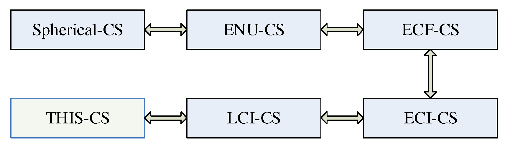
The last step of coordinate transformation from the LCI-CS to the THIS-CS defined in
Figure 1 is
where
. Note that the difference between the LCI-CS and THIS-CS is the translation of the origin by range
and the rotation of the CS by angle
.
Figure 2 gives the flow chart of the above-mentioned coordinate transformations, which is relatively complicated. The rudimentary operations are translations and rotations.
Substitution of Equations (16)–(23) into Equation (24) and collections of terms yield the following equation:
where the transformation matrices are expanded as follows
The full expansions of the above matrices are
Up to this point, Equation (25) has built up the interrelationship between raw radar measurements
and the elliptical vector
. If all the relevant parameters are correct, the projection of the raw observations onto the THIS-CS defined in this paper will be a part of an elliptical curve and in a plane. The full expansion of
is considerably complicated, but it can still be reformulated as the following form
where
is a nonlinear vector function. Or equivalently, we have the implicit equation
Note that in Equation (33) the measurement is , which is usually limited to a preconditioned surveillance region D, and can be obtained directly by the radar with some measurement errors, whereas the parameters are usually unknown and need to be determined. This is also the focus of our investigation. A simple way to implement the EHT is to map the 3-D raw data into a 7-D parameter space and to make an exhaustive search. Since higher search dimensionality (7-D) requires much more processing load and data storage, and it is not easy to implement in real time, one must resort to some heuristic approaches to reduce the search dimensionality in the first place.
These parameters can be divided roughly into two groups: elliptical parameters and reference parameters . Elliptical parameters are those, in essence, related to the thrust-cutoff parameters and are the parameters we must search via a voting scheme in the parameter space, whereas the reference parameters are not essential and can be roughly obtained by an early-warning radar (or by an early-warning satellite) as apriori.
If the early-warning information is not available, some heuristic methods can also be developed to estimate these parameters. For instance, , in essence, determines that in the THIS-CS. Considering the factor of noise, we can search by minimizing the sum of the absolute value . Furthermore, note that the thrust-cutoff point is only a reference point, which is not unique and dependent on the altitude at the thrust cutoff point. For a common practice, is a reasonable reference value. Thus, the final reference parameters might be reduced to two-dimensions, i.e., and . If the early-warning information is not available, three independent standard polynomial Hough transforms can be used to detect in the separate , , and planes. The detection results are then combined and transformed to the geodetic CS; the extrapolated value at altitude is the requisite reference thrust cutoff point.
In the following sections, for the sake of conciseness and due to space limitations, we assume that the early-warning information is available, but with some estimation errors. Thus, the main work is focused on the search scheme for the elliptical parameters , and . Actually, according to Equations (13) and (14), it can be seen that , and are not independent. Known any of the two, then another parameter is obtained. However, it is difficult to use Equations (13) and (14), since in most cases is usually applied at first. Equations (13) and (14) can be used as constraints to greatly reduce the huge search space.
4. Elliptical Hough Transform
4.1. Data Space and Parameter Space
Note that before transformation Equation (24), all the data expressed in the LCI-CS are explicitly known, except for some measurement errors and early-warning parameter-related errors. However, the transformation Equation (24) is still ambiguous since θ is an undetermined parameter, which must be searched over all possible discrete values, together with the search of parameters and .
In fact, if we denote
as a new vector, then the LCI0-CS can be viewed as the LCI-CS, translating from the cutoff point A to the Earth center
. The vector
is also a known quantity related to the measurements.
Using
to represent Equation (2) and expanding the rotation matrix
, we obtain the three-parameter elliptical equation as
Thus, the EHT maps the points
in the converted data space into curves in a
three-parameter space. Note that, when discussed here,
are the state variables, whereas
are the parameters. According to Equation (35), it is difficult to judge the curve type in the Hough parameter space. Instead, we use the vector in the THIS-CS to analyze its properties. Using the coordinate relationship
to replace Equation (35), it follows from that Equation (35) can be rewritten as
Thus, for a given value , the vector in THIS-CS can be explicitly computed by using Equation (36); then, the data mapping Equation (37) results in a planar quartic curve, instead of an elliptic curve.
It can be seen that any one of the quartic curves in the Hough parameter space corresponds to the set of all possible elliptical curves in the data space in the THIS-CS through the corresponding data point. If an elliptical curve of points does exist in the THIS-CS, the curve is represented in Hough parameter space as the point of intersection of all of the mapped quartic curves, i.e., in the parameter space, multiple quartic curves will gather at a point, and the parameters at this point are the desirable ones we are searching for.
4.2. Algorithm Design
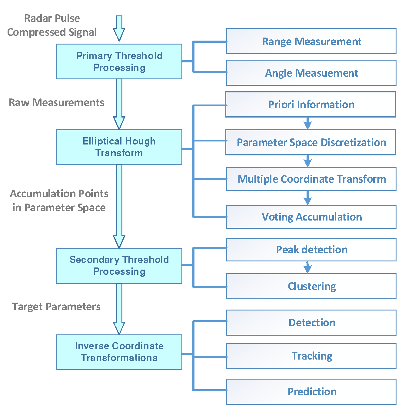
Next, we give full steps of the algorithm design for the presented EHT. The basic idea is illustrated in
Figure 3, and it has four main parts.
- (i)
Primary Threshold Processing: The radar operates in a TBD mode, searching a limited number of sectors (surveillance region) . The search is implemented via a sequential mode, i.e., every resolution cell in the region is scanned only once during a search frame time . The radar raw pulse compressed signals (range-azimuth-elevation channels) are through a much lower primary threshold . In this way, we obtain the original measurement points , although this dataset contains quite a lot of clutter.
- (ii)
Elliptical Hough Transform: Firstly, the values of the reference parameters, as well as the rough bound of the elliptic parameters, are obtained from the apriori information. The parameter space is then quantized in the dimensions. Any cell with a value exceeding is mapped into parameter space via multiple steps of coordinate transformation, and its power is reset to count 1. When a primary threshold crossing is mapped into the parameter space, its power (note, we use a binary integrator; hence, its power is 1) is added into the cells that intersect the corresponding quartic curve in the parameter space. In this way, the accumulator cell at the intersection of multiple quartic curves will have a high value; this is called voting accumulation.
- (iii)
Secondary Threshold Processing: A secondary threshold can be applied in the parameter space to declare detections of targets of interest. Note that if the secondary threshold is set too low, there might be multiple detection scatters in neighboring parameter cells. In fact, there indeed may be only one target; it is the quantization of parameter space that leads to the false alarm. To reduce false alarms and meanwhile obtain fine estimation accuracy of the desired parameters, a clustering method can serve this purpose.
- (iv)
Inverse Coordinate Transformations: The detected elliptical parameters are back-transformed into the measurement space by a series of inverse coordinate transformations, and both detection and tracking results are announced to show the time history and current position of the target. Meanwhile, it is very easy to use the detected parameters to predict the long-term evolutionary behaviors of the trajectory. For instance, the intersection between the detected trajectory and the Earth’s surface is the landing point.
The detailed algorithm to implement the EHT is listed as follows:
Step 1: Search the surveillance space sequentially and store the frame raw measurement data. If the power of one cell exceeds the primary threshold , then its position is recorded. Thus, during the time interval , we obtain the total measurement data , wherein the frame has measurements, and the total number of measurements in the processing period is .
Step 2: Discretize the three-dimensional parameter space
(the parameter discretization region can be obtained according to the early warning or determined by experience), and obtain
cells. The parameter resolutions are
and the parameter values can be obtained as
Set the initial accumulation variable as
Step 3: For every
and every data
total number
m), use the apriori information of early warning
to calculate the converted data
via Equation (25). Thus, we have
Step 4: For every
and every
, compute the semi-minor axis
Step 5.1:
Scheme I (
Binary integration): For every
and every
, if
subjects to
Then, the count of the accumulation cell
is added to 1, i.e.,
Step 5.2:
Scheme II (
Plane-constrained integration): For every
and every
, if
subjects to Equation (42), then the accumulation steps change to
where
q is a design coefficient.
Step 6: Set the secondary threshold
in the Hough parameter space, if
, we obtain a detected cell, and the estimation parameters are obtained as
,
, and
. In certain cases, the detections might be multiple and scatter in several adjacent regions. A k-means clustering method or hierarchical agglomerative clustering method [
48] can be employed to combine the neighboring detected cells into one cell.
Step 7: Suppose ultimately that we have detected targets with parameters . Using a series of inverse coordinate transformations indexed by Equation (37) back to Equation (15), we can retrieve the positions of targets of interest in any desirable CS. In this way, the presented EHT method declares the detection and tracking results simultaneously. Furthermore, it is also possible to use the estimated parameters to predict the long-term trajectory of the targets to be detected.
Note that, in Equation (44), we have considered the fact that the orbit of an exoatmospheric target in the midcourse usually follows a planar trajectory, hence might be sufficiently small if the target turns out to be the true one. However, for random thermal noises or clutter, they would uniformly intersperse in the surveillance space and might have large values for . Therefore, for Scheme II, it indeed has the advantage of improving the accumulation performance for true targets, as well as reducing the false-alarm rate for noises. When in the case , , Scheme II will reduce to Scheme I, whereas when we will have . For the latter case, both targets and noises have no accumulation effect. Because remains a design parameter, in this investigation, we find that when it might have better accumulation performance.
Now we analyze the computational complexity of the EHT. The points in the measurement space correspond to a quadratic curve in the parameter space. Using apriori information to partition the parameter search space, we obtain a total of quantized parameters. Assuming that the total number of measurements is during N-frame scan, then in theory, the total of cumulative calculations will be performed. In fact, since have the constraint relationship Equation (37), b does not need to be quantified, and the total computation is . It follows that the more the number of targets, the denser the clutter, the longer the accumulation time, and the higher the accuracy of parameter quantization, the more time consuming the algorithm is.
Furthermore, in the above steps, we have used a three-dimensional search parameter space
instead of two-dimensional space
indicated by Equations (13) and (14). Since Equations (13) and (14) are relatively computationally sophisticated, we only use them as a constraint to reduce the number of search points. That is to say, when implementing the step of discretization Equation (39), we select only the points that satisfy Equations (13) or (14) to implement the mapping. Using Equation (14) as an example, the selection is judged as
where
is the measurement-related computed value of
,
is the theoretical computed value of
according to Equation (14), and
is introduced to account for all types of measurement errors. With the steps of preselection, unlike pairs of
can be greatly reduced.
4.3. Detection and False Alarm Probabilities
Next, we analyze the statistical performance of the EHT.
The thermal noise-induced false alarm is considered as Rayleigh distributed in amplitude or exponential in power. Assuming a square law cell detector, then the normalized power probability of distribution (pdf) of noise is
For the sake of simplicity, we assume the exoatmospheric target follows a Swerling II distribution. Note that in reality, it is rarely the case that a reentry vehicle follows a classical Swerling model; instead, it depends on a lot of elements. Herein, since the Swerling II model has the simplest analytical expression of the probability of detection , we use it only to give a clear picture of the statistics of the method. Note that any other target fluctuation models are also applicable to this analysis.
The power pdf of the target is
where
is the SNR. It is easy to obtain the
for single
detection cell as
where
is the primary threshold, with
the probability of false alarms for noises. Obviously, the larger the value of
is, the lower the threshold
will be. To guarantee the subsequent Hough detection of a target, the primary threshold
should be set relatively lower.
To obtain the final probability of detection
per Hough parameter space cell, we follow the same way originated from Carlson [
17]. Let
n be the total number of
cells that can contribute to a given parameter space cell. There are total
data points exceeding the primary threshold
. Thus, the probability of this event is
, where
is in essence the maximum accessible number for a given Hough parameter cell. According to [
17], we directly give the probability
that a given cell in parameter space exceeds the secondary threshold
as follows:
where
denotes the accumulation power for this given parameter cell and
is the power of the
data point. Actually, for binary integration (Scheme I),
; whereas for plane-constrained integration (Scheme II),
. Obviously, for Scheme I, the final probability of detection is reduced to
where
denotes the rounding operation. The
for Scheme II is obtained as
Note that it is difficult to obtain the analytical expression since the accumulation statistic has a sophisticated distribution. For the sake of conciseness, we do not go into the details of the detection and false alarm probabilities in this investigation. Once is available, the false alarm probability can be obtained by limiting .
Actually, the detection performance relates to many elements, such as the primary threshold , secondary threshold , SNR, resolution cell of discretization , total processing Plane-constrained integration NΔt, radar measurement errors, and estimation accuracy of early-warning information, etc. Most of these statistics do not have analytical expressions and need massive Monte Carlo simulations to give a quantitative evaluation.
5. Simulations
In this section, we consider an example of a single search radar scenario and investigate the performances of the presented EHT algorithm.
5.1. Scenario Description
The simulation scenario is depicted as follows.
Target: We assume a single reentry vehicle flying in the exoatmospheric phase. The initial reference velocity, altitude, and tilt angle at the thrust cutoff point are 2500 m/s, 80 km, and 40.3070°, respectively, which subsequently determine the total exoatmospheric flight time of approximately 370 s. At the reference time , the target is located at 0° N latitude 0°E longitude, pointing to the direction of East. The apogee is 0°N latitude 3.03485°E longitude, and the reentry point is 0° N latitude 6.0697° E longitude.
Radar: The radar is positioned at 2°N latitude 4.5°E longitude with a scan period . The measurement accuracies of range, azimuth, and elevation are and , respectively. The radar has received some apriori early warning information from the satellite; thus, the surveillance space is restricted to a limited region of km3. The processing time interval is [150, 250] s. Thus, the accumulation frame number is , which accounts for a total data time of about 100 s.
False alarm: The number of false alarm detections is Poisson distributed with a spatial density /km3, which determines an average number of 18 false alarms of a single scan in the surveillance space D. Note that is essentially a function of the cell false alarm probability of the radar and is independent across frames.
Early warning information: The true reference parameters provided by the early warning are , , , and . The indicated errors are assumed to be Gauss distributed with standard deviations and .
EHT specification: The Hough search space is restricted to , , and , with a resolution , , and . The total quantization points are approximate 8 × 10⁶. The judgment of the successful detection of a target is set as and . Note that the threshold of judgment remains a design parameter in practice, adjusted/tuned mostly based on engineering experience and intuition. Actually, the optimal threshold is difficult to derive as it is related to specific radar-target geometry and related to many issues.
5.2. Raw Measurements
The radar measurements are available in radar spherical CS at discrete time instants.
Figure 4 shows the true target and radar raw measurements in the preconditioned surveillance space
D, with
Figure 4a the measurements in the radar raw PPI display and
Figure 4b the converted measurements in THIS-CS defined in this paper. It can be seen that, while the trajectory of the target in the PPI display is a continuous and complicated curve, in the THIS-CS it indeed is a part of the elliptical curve and symmetrical with the Earth center.
Note that in
Figure 4 we do not consider the SNR. The gray-scale plot of all 200-frame primary threshold detections is shown in
Figure 5, with darker points denoting higher power. Actually, the threshold
means an average SNR of 10 dB. It can be seen that the target is more visible as an elliptical curve, but it scatters in a cluttered environment. Conventional recursive trackers usually need an average SNR of 20 dB sufficient to maintain the track, and in this low SNR case, they may lose tracks due to frequent misdetections of the target erroneously associated with unwanted clutter points.
5.3. Integration Effects
Figure 6 and
Figure 7 show the accumulation effects in the Hough parameter space, with
Figure 6 for Scheme I, Binary integration, and
Figure 7 for Scheme II, Plane-constrained integration,
. The target SNR is still 10 dB and the primary threshold is
. For the sake of compactness, we do not show the accumulation effect in the
dimension, since it has similar behaviors. It can be seen from
Figure 6a and
Figure 7a, in the parameter space, we did observe that multiple quartic curves gather together.
The two schemes can concentrate both on the true parameters , but their accumulation effects have slight differences. It can be observed that Scheme II has a better accumulation effect than Scheme I. The reason partly lies in that Scheme II has sufficiently considered orbit planarity as a constraint, wherein the noises located outside the orbit plane have been largely suppressed. For this reason, in the following analysis, unless stated explicitly, we will use Scheme II, i.e., Plane-constrained integration to implement the EHT.
5.4. Parameter Estimation
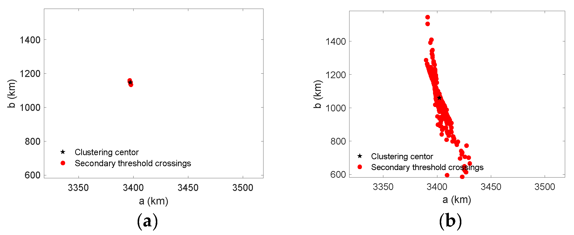
With the K-means clustering, we can obtain the ultimate estimations of Hough parameters for the EHT.
Figure 8 shows the estimated parameters of the EHT with different secondary thresholds
and
, wherein the symbol “★” denotes the clustering center and “·” denotes the secondary threshold crossings. It can be seen that, when the Hough threshold
is relatively high, only a few points can pass the threshold, and the estimation accuracy of parameters will be satisfactory. However, this is not the case for a lower threshold. In
Figure 8b, the secondary threshold is set to
, and we can observe that the clustering center deviates vastly from the true value.
Once the parameters in the Hough parameter space are obtained, they can be mapped back into the measurement space
R −
A −
E −
t or any other CSs, to show the time history and current position of the target.
Figure 9 shows the corresponding detected curve, true trajectory, and raw measurements in a single plot, with
Figure 9a the detection threshold
and
Figure 9b
. It can be seen from
Figure 9a that, the presented EHT works well as the detection result approximates highly to the nominal true trajectory. In contrast to
Figure 9a,
Figure 9b shows that it has worse detection performance. Because its secondary threshold is relatively low, multiple crossings will be recorded and this will reduce the clustering performance. However, in reality, the secondary threshold
is still a key design parameter and needs to be determined by experience or massive Monte Carlo simulations.
5.5. Performance Comparison
Next, we investigate the detection performance due to the influence of the primary threshold, secondary threshold, radar measurement error, and SNR. This is achieved by massive Monte Carlo runs. In the following simulations, the accumulation time interval is still restricted to [150, 250] s. To assess the performance of the proposed method, 10,000 Monte Carlo numerical simulations were performed in Matlab® on a computing platform characterized by a 3.6 GHz Intel Core I7–4790 processor with 32 GB RAM.
Figure 10 shows the detection performance concerning the primary threshold
and SNR.
Figure 11 shows the detection performance concerning the secondary threshold
and radar measurement errors.
From
Figure 10 and
Figure 11, some conclusions are obvious. We briefly summarize them as follows:
- (i)
The larger the SNR is, the higher the detection probability obtained;
- (ii)
The lower the primary threshold is, the higher the detection probability obtained;
- (iii)
The higher the secondary threshold is, the higher the detection probability obtained;
- (iv)
The higher the radar measurement accuracy is, the higher the detection probability obtained.
Note that in
Figure 11, it does not mean that the higher the secondary threshold, the better. It can be observed that, when
is set too high to cause no secondary threshold crossings, it may result in missing alarms, and consequently decrease the probability of detection. Alternatively, one can set no secondary threshold and assume that the peak value corresponds to the desired target. However, this may also induce false alarms, since even if there is no target, the detector will still declare a target.
In fact, the detection performance relates to many elements, such as the primary threshold , secondary threshold , SNR, resolution cell of discretization , total processing time interval , radar measurement errors, and the estimation accuracy of early-warning information. Most of the statistics do not have analytical expressions and need massive Monte Carlo simulations to give a quantitative evaluation.
Table 1 shows the average running time of the EHT method with different parameters. The primary false alarm probability is varied in the range
and the parameter space quantization in the range
. The target accumulation time interval is still restricted to [150, 250] s. As seen in
Table 1, the computational load of the algorithm does increase as the primary detection threshold decreases and the number of quantization units increases. Nonetheless, this processing time is still within the total accumulated time. The total running time will also be greatly reduced if a parallel processing strategy and hardware computational platform are used.
Next, we investigate the performance in a very low SNR environment.
Figure 12 gives the detected curves in the THIS-CS with an average SNR of 0 dB, which means that the primary threshold is very low, and most of the clutter points will contribute to the Hough space accumulation, while that of the target points will be greatly decreased. The other parameters are Scheme II, Plane-constrained integration, with
, time interval (150–250) s, primary threshold
η = 0, and secondary threshold
.
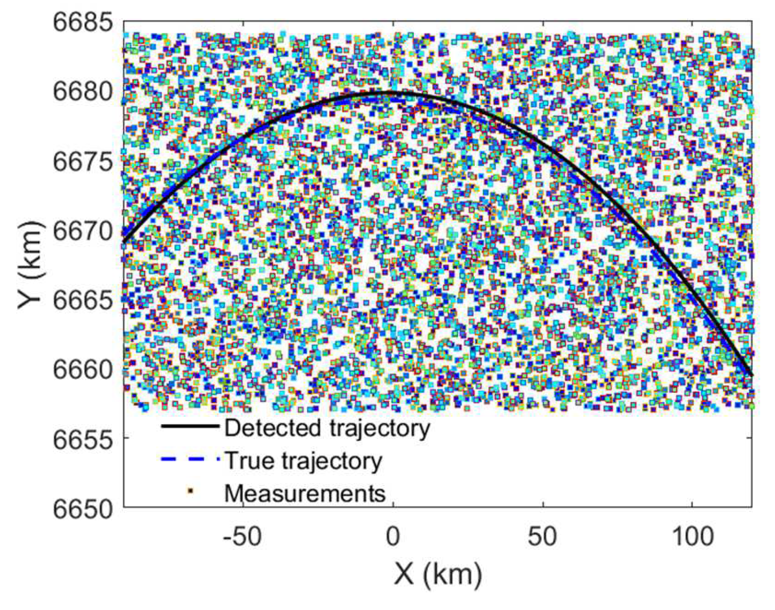
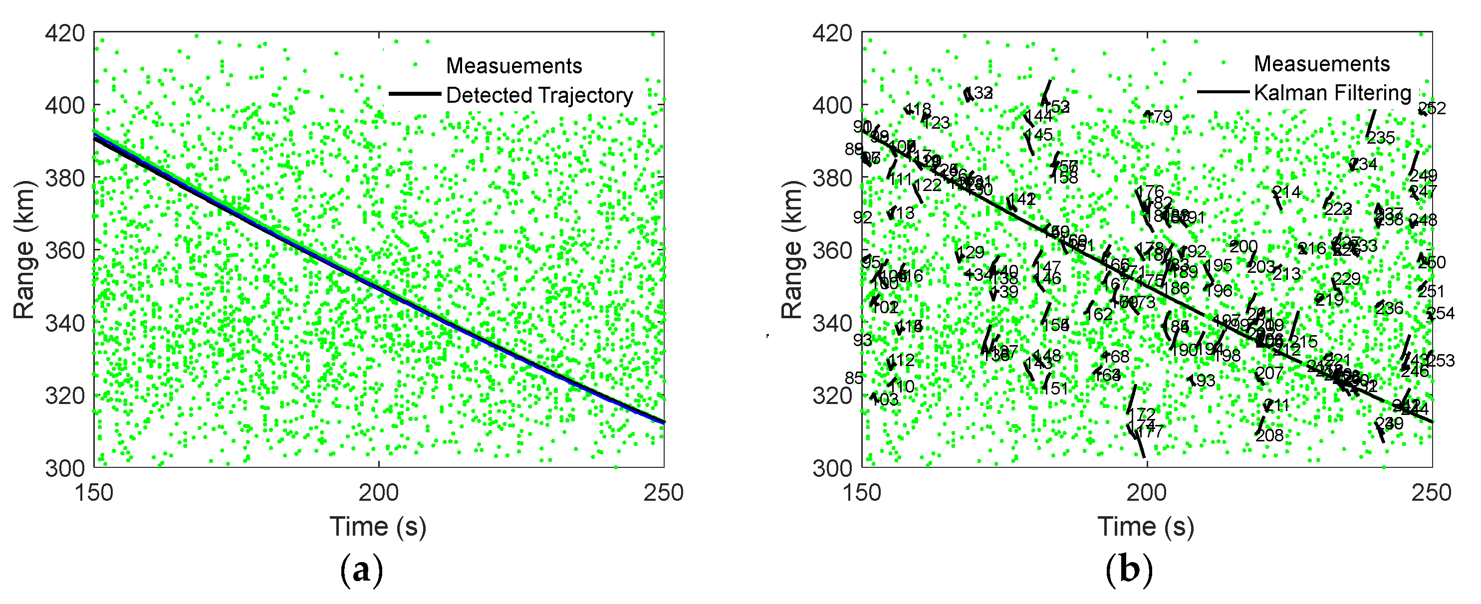
Transforming
Figure 12 to the radar raw R-A-E measurement space with inverse coordinate transforms, we obtain the detection and tracking results. As shown in
Figure 13a, the detected trajectory of ETH highly coincides with the true value. The ETH is a TBD method since detection and tracking are announced simultaneously. In fact, although the primary threshold is lowered and the clutter becomes massive, this also means that the probability of detection of the target becomes higher. In order to compare the performance,
Figure 13b shows the tracking results of traditional data processing via a detect-before-track (DBT) mode. In
Figure 13b, the track initialization is three-point differentiation, the association algorithm is nearest neighbor (NN), and the filtering algorithm is interacting multiple model (IMM). The filter parameters are adjusted to the best. Nevertheless, as can be seen from
Figure 13b, the traditional DBT method tracks a large number of temporary tracks. Specifically, the tracks of the target are often intermittent. In fact, there are a total of 18 tracks that belong to the same target, and the total number of temporary tracks reaches 253. This not only wastes radar tracking resources, but also poses a challenge for subsequent target discrimination.
Figure 14 gives the accumulation effect of multiple targets, with
Figure 14a the accumulation effect in the Hough parameter and
Figure 14b the detection result in THIS-CS. The parameters are still Scheme II, Plane-constrained integration, with
, time interval [150, 250] s, primary threshold
, and secondary threshold
. The difference between these two targets is the difference in release altitude of 10 km. As can be seen, our method can also detect multiple targets at the same time. In fact, the Hough transform is based on a voting mechanism where the accumulation between targets is independent; thus, the Hough transform has implied parallelism, as well as multi-target detection capability. We also find through simulation that our method is able to detect the same target even if the trajectory passes through the surveillance area and then returns to the surveillance area.
5.6. Field Data Analysis
To evaluate the effectiveness of the presented EHT method, we also use filed data to investigate the overall performance. The radar is a phased-array radar, which is manufactured by the China Electronics Technology Group Corporation (CETC) and is operated at the X-band. The data we analyzed involves a constellation comprising three identical scientific satellites of the European Space Agency (ESA), which are designed to provide the best survey of the geomagnetic field and its temporal evolution of the Earth system.
To meet the need for the detection accuracy of the magnetic field of the Earth system, the satellite constellation consists of three circular orbits, with satellites A and C approximately 450 km above the ground, and satellite B 530 km above the ground. Because these data span different periods, we use only the real tracking data of satellite A to investigate the performance. The shape of satellite A is shown on the left of
Figure 15.
The orbital elements of satellite A are listed in
Table 2. It can be seen from
Table 2 that, the trajectory is approximately a part of a circular orbit, as the eccentricity
is close to zero. According to the basic knowledge of astronomy, we can calculate the true elliptical parameters (
a,
b,
θ) = (6811.4487 km, 6811.4483 km, 0°). Since the target is a satellite and it has a circular orbit, the range angle
indeed can be of any value.
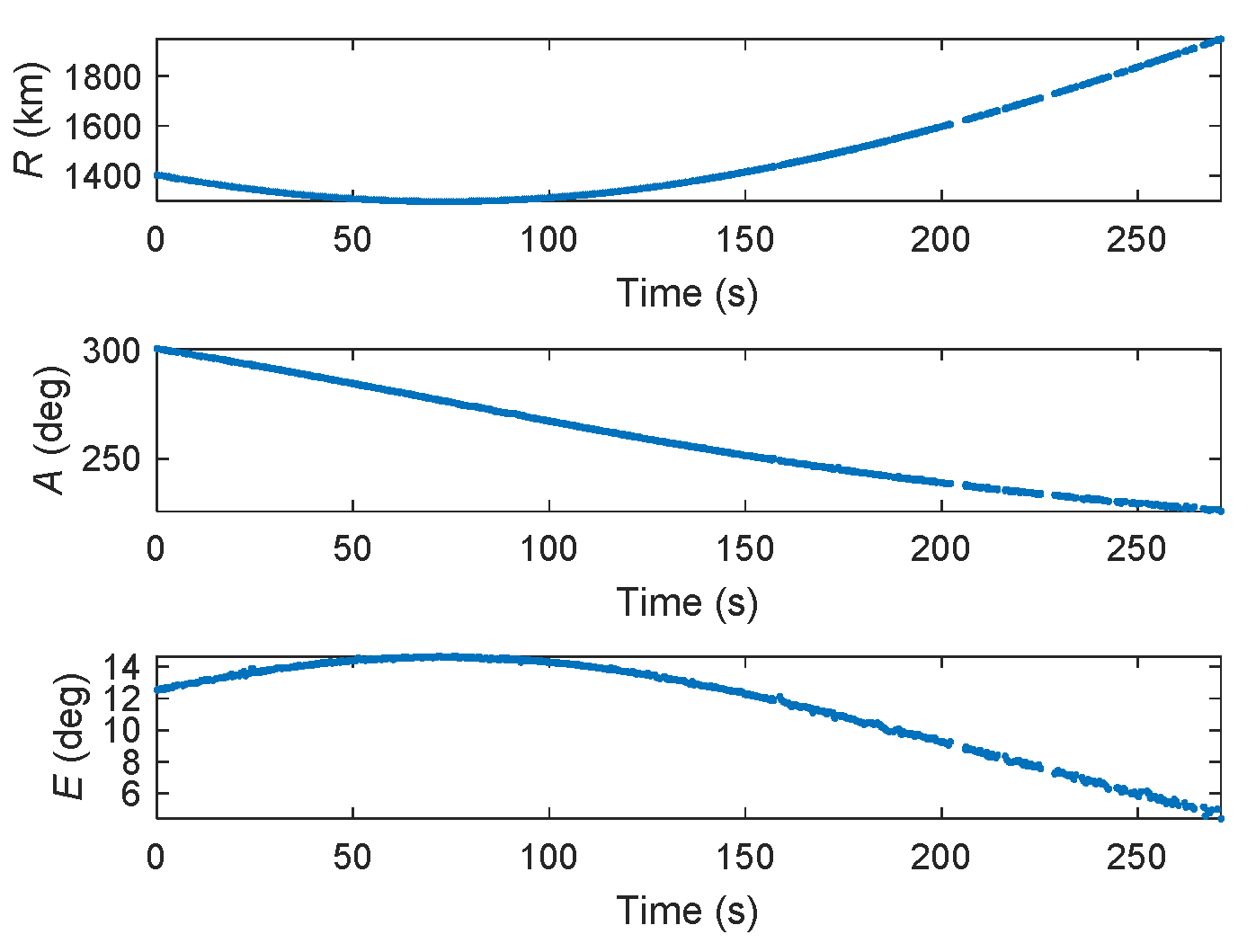
Figure 16 shows the raw measurements of the satellite when tracked in the radar centered spherical CS. The data is collected on 8 May 2017. The total observation time is approximately 272 s of its exoatmospheric flight, with the range in the interval [1296 km, 1950 km], azimuth in the interval [225.7384°, 300.6767°], and elevation in the interval [4.4123°,14.6599°]. Since the radar is a phased-array radar and has the ability of adaptive scheduling, the maximum revisiting period is 3.94 s, the minimum period is 0.067 s, and the average is 0.5 s. The measurement accuracies of the range, azimuth, and elevation of the radar are approximate
,
, and
, respectively.
With a series of coordination transformations, the satellite trajectory in the presented THIS-CS can be obtained. As can be seen in
Figure 17, the trajectory of the orbit is indeed a part of a circular orbit, with an average height of approximately 449 m. Due to the radar line-of-sight limitation, the radar can only observe a small part of the entire circular orbit.
Since the raw data set is the independent tracking data containing the raw measurements of range, azimuth, and elevation, and for some reason lacking the SNR information, obviously, it cannot be used directly to evaluate the performance of the elliptical Hough transform, as the Hough transform usually needs target data, as well as clutter data.
To investigate the algorithm performance in stressful environments, we add some imaginary (non-real and man-made) clutter data, combining the raw satellite data to constitute a simulated cluttered environment.
The number of clutter detections is still assumed to be Poisson distributed with spatial density /km3, which determines an average number of 18 false alarms of a single scan in the surveillance space.
Thus, the field data are preprocessed with the following steps: adding clutter data (imaginary), implementation of the elliptical Hough transform, and inversion to the original CS.
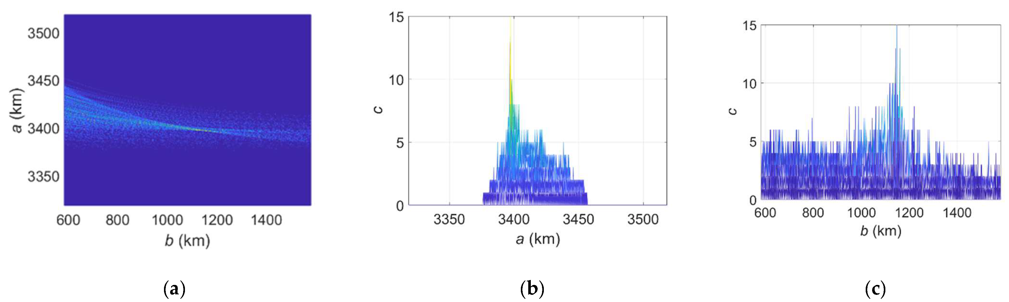
Figure 18 shows the accumulation effects in the Hough parameter space of the synthetic data. The parameters are Scheme II, Plane-constrained integration with
, time interval [0, 272] s, and average SNR = 10 dB. The other parameters are assumed to be the same as earlier. It can be seen from
Figure 16 that the corresponding quartic curves intersect at some point and have a high value in the parameter space. In fact, by setting the secondary threshold
and using the K-means clustering method, we obtain the detected elliptical parameters
, which are now very close to the true values
.
Once the parameters in the Hough parameter space are obtained, they can be converted back into the measurement CS or any other CSs to show the time history and current position of the target.
Figure 19a shows the corresponding detected curve, assumed (imaginary) clutter, and raw satellite measurements in the THIS-CS, while
Figure 19b shows the same result in the radar-centered ENU-CS. It can be seen from these two figures that the EHT works well, as the detected trajectory approximates highly to the true measurements of the satellite. An interesting fact in
Figure 19 is that there seems to be a fixed deviation in the detection process. Even without adding any clutter (using the original tracking data), this fixed deviation will still exist and cannot be ruled out. The reason partly lies in the fact that a spherical Earth model is employed, which might result in systematic errors and cannot reflect the truth. Perhaps adopting a more precisely ellipsoidal Earth model would mitigate this effect, and this needs further investigation.


