Article

GMT-WGAN: An Adversarial Sample Expansion Method for Ground Moving Targets Classification

Key Laboratory of Electronic Information Countermeasure and Simulation Technology of Ministry of Education, School of Electronic Engineering, Xidian University, Xi’an 710071, China
*
Author to whom correspondence should be addressed.
Remote Sens. 2022, 14(1), 123; https://doi.org/10.3390/rs14010123
Submission received: 10 November 2021 / Revised: 17 December 2021 / Accepted: 25 December 2021 / Published: 28 December 2021
(This article belongs to the Special Issue Radar High-Speed Target Detection, Tracking, Imaging and Recognition)

Abstract

:
In the field of target classification, detecting a ground moving target that is easily covered in clutter has been a challenge. In addition, traditional feature extraction techniques and classification methods usually rely on strong subjective factors and prior knowledge, which affect their generalization capacity. Most existing deep-learning-based methods suffer from insufficient feature learning due to the lack of data samples, which makes it difficult for the training process to converge to a steady-state. To overcome these limitations, this paper proposes a Wasserstein generative adversarial network (WGAN) sample enhancement method for ground moving target classification (GMT-WGAN). First, the micro-Doppler characteristics of ground moving targets are analyzed. Next, a WGAN is constructed to generate effective time–frequency images of ground moving targets and thereby enrich the sample database used to train the classification network. Then, image quality evaluation indexes are introduced to evaluate the generated spectrogram samples, with an aim to verify the distribution similarity of generated and real samples. Afterward, by feeding augmented samples to the deep convolutional neural networks with good generalization capacity, the classification performance of the GMT-WGAN is improved. Finally, experiments conducted on different datasets validate the effectiveness and robustness of the proposed method.

Graphical Abstract

1. Introduction

The detection and classification of ground moving targets have been widely applied to military and civilian applications, such as square surveillance, airport scene surveillance, post-disaster rescue, anti-terrorism, and auxiliary medical treatment, and have been widely researched [1,2,3,4,5,6,7]. Pedestrian and vehicle targets are the main types of surveillance objects of a ground surveillance radar. The Doppler effect occurs when there exists a relative motion between the target and radar. When the radial motion speed of a ground moving target is slow, the target Doppler spectrum and clutter spectrum can easily overlap, which increases the difficulty in detection and recognition of pedestrian and vehicle targets. At the beginning of this century, Chen’s team from the Naval Research Laboratory of America systematically studied the micro-Doppler effect of radar [8]. A target or some of its parts have a relative movement (e.g., vibration, swing, or rotation) to the main body, which is the main cause of the micro-Doppler effect. The micro-Doppler frequency produces sidebands around the Doppler shift and widens the main Doppler spectrum [9]. If micro-Doppler information is introduced, the detection and recognition probabilities of ground moving targets, such as pedestrians and vehicles, can be improved significantly. Therefore, the classification and recognition of ground moving targets based on micro-Doppler characteristics have attracted great attention in recent years and have become one of the main research topics in the area of target classification [10,11].
Pedestrian movement is a highly coordinated non-rigid movement, which includes the action of the brain, muscles, nerves, joints, and bones. It has a non-stationary property of a single scattering point and a non-rigid property of multiple scattering points. There are three ways to obtain the radar echo. The first way is by using pedestrian motion modeling based on the biomechanical model. A typical model is the Boulic model [12], which was developed to imitate pedestrian walking to calculate the speed of human joints. In [9], the authors improved the Boulic model, simulated the radar echoes of pedestrian walking, analyzed the micro-Doppler effect of pedestrians through the time–frequency analysis, and estimated the arm swing frequency and gait cycle. However, this method mainly aims at the ideal walking model and has a low generalization ability. The second way is through pedestrian motion modeling based on the motion capture (MOCAP) data [13]. In the work of Barrs Erol et al. [14], a few complex motion models were established by directly capturing the pedestrian motions, which recorded the actual motion trajectory of each node of the human body. In the work of Yao et al. [15], the authors improved the MOCAP model, simplified the model, and improved the modeling efficiency on the premise of meeting the real motion requirements. In this method, the motion modes are diversified, but the scattering characteristics are still different from the actual situation. The third way is to record the actual, measured radar echo data. In the work of Björklund et al. [16], the authors used a 77 GHz radar to record the pedestrian posture echoes and applied the micro-Doppler characteristics of pedestrian postures to multi-person recognition. In the work of Mehul et al. [17], a continuous gait was collected by a frequency-modulated continuous wave radar and three ultra-wideband (UWB) pulse radars placed at different locations. However, this method is difficult to use in practical situations and has high requirements for the hardware equipment.
Considering the pedestrian activities recognition, in the work of [18], Garreau et al. classified pedestrians, skiers, and cyclists using a classifier based on their differences in micro-Doppler characteristics. In the work of Lshibashi et al. [19], a classifier that can simultaneously classify the lifting action and its load weight based on the kinematic quantities of the body motion was developed using the hidden Markov model framework. In the work of Fairchild et al. [20], different classifiers were used to distinguish various pedestrian movements. In the work of Amin et al. [21], pedestrians on crutches were identified. In the work of McDonald et al. [22], humans sitting in a taxiing plane were identified. In the work of Kim et al. [23], the physical characteristics of pedestrians was used to detect them. In the work of Bryan et al. [24], the micro-Doppler characteristics of pedestrians were analyzed using a UWB radar. In addition, many classification methods, such as support vector machine [25], have been used to achieve better classification results of running, walking, armed walking, climbing, and other types of motions. In the work of [15], Yao et al. used a complex-valued neural network to classify pedestrian activities, extracted more rich features, and achieved higher classification accuracy under the small-sample conditions and a low signal-to-noise ratio (SNR) environment. Considering the classification of pedestrian and vehicle targets, in the work of Nanzer et al. [26], the difference in the number of strong scattering points in the time spectra of the pedestrian and vehicle targets was used to classify these two types of targets. In the work of Du et al. [27], the micro-Doppler characteristics of pedestrians and vehicles were studied based on the measured continuous wave radar data, and noise reduction and clutter suppression of measured data were performed by the Bayesian learning method; robust features extracted from the time–frequency spectrum were used to classify pedestrians and vehicles. In the work of [28], Shi et al. analyzed differences in the micro-motion characteristics of pedestrian and vehicle targets and extracted the spatial features of the spectrogram, namely, the texture characteristics; good classification results were achieved.
All the above-mentioned classification methods are based on manual feature extraction, and different classifiers have been used to classify the ground moving targets. However, these methods heavily rely on prior knowledge that has strong subjective factors and can be applied only in specific application scenarios due to their low generalization ability. With the development of hardware equipment, more attention has been paid to deep-learning-based methods, which can automatically extract inherent characteristics of targets without requiring prior information and can achieve good classification performance. In the works of Kim et al. [29,30], a convolution neural network based on the micro-Doppler analysis was used to classify and recognize pedestrian motions. Although common deep-learning-based methods can achieve good recognition results, they require a large number of training and testing samples; if there are fewer samples, they are likely to overfit, which reduces their classification performance. Therefore, it is necessary to enhance and augment the training samples. In the work of Du et al. [27], the number of samples was increased through sliding window processing; however, its generated samples had a strong similarity. In the work of Bjerrum et al. [31], a data enhancement method based on affine transformation, which can generate similar samples by enlarging, reducing, translating, and rotating a sample image, was proposed. In the work of Song et al. [32], an image sharpening method was used to enhance the training sample set. However, these image transformations are global and can neither focus on the diversity of local regions nor extract the intrinsic features of a database. In the work of Goodfellow et al. [33], a generative model was proposed based on the game process of generator and discriminator, namely generative adversarial network (GAN), which can reach the Nash equilibrium and generate new images with similar but different features to the original images. In the work of Seyfioğlu et al. [34], a self-encoder was used to initialize network parameters in the case of small samples, and then a convolutional network was used to classify auxiliary and non-auxiliary indoor pedestrian movements, and good classification results were achieved. In the work of Alnujaim et al. [35], a GAN was used to supplement the pedestrian micro-motion data collected by a Doppler radar, which solved the problem of insufficient training data and improved the deep convolutional neural network (DCNN) classification accuracy. In the work of Erol et al. [36], a pedestrian micro-motion data enhancement method based on the auxiliary condition GAN was proposed for the classification of pedestrian activities. However, the data generated by this method need to be processed by the principal component analysis to eliminate inconsistent samples. In the work of Alnujaim et al. [37], a GAN was used to expand the time–frequency (TF) images obtained from a single angle into images from multiple angles, thus enriching the sample set from multiple perspectives. However, a GAN has the limitation of convergence instability, which makes it be prone to produce samples with high similarity. To solve these problems, the Wasserstein GAN was proposed by Arjovsky et al. [38], and has been applied in some research. In the work of Magister et al. [39], the WGAN with a semantic image inpainting algorithm was used to devise more realistic retinal images for medical teaching purposes. In the work of Fu et al. [40], a novel framework by concatenating a super resolution GAN and a WGAN was proposed to increase the performance of a backbone detection model.
To obtain good performance of ground moving targets classification under small sample conditions and solve the problem of limitation of convergence instability, a WGAN sample enhancement method for ground moving targets (GMT-WGAN) classification is proposed in this paper.
The proposed method augments the samples using the adversarial learning strategy and increases the richness of information under the condition of small samples. Compared with the existing ground moving target classification methods, the main contributions of the proposed GMT-WGAN method are as follows:
(1) Wasserstein distance is introduced to measure the difference between the real and generated distributions of the ground moving targets in the adversarial network, which makes the training more stable, and the training degree of generator and discriminator is no longer needed;
(2) The inverse of the Wasserstein distance is used as a loss function of the discriminator in the ground moving target samples generation, which can indicate the training process state;
(3) Three different databases are established to verify the effectiveness of the proposed method. Experimental results show that the GMT-WGAN method can provide significant improvement in the ground moving target classification under different SNR conditions.
The remainder of this paper is organized as follows. Section 2 introduces the related work of the GMT-WGAN, including the motion characteristics of ground moving targets, the time–frequency analysis method based on the short-time Fourier transform, and the basic principle of the GAN. Section 3 presents the proposed GMT-WGAN method. Section 4 provides detailed experimental results and evaluates the sample image quality of the WGAN. Section 5 concludes the paper.

2. Related Work

2.1. Ground Moving Target Motion Characteristics

Ground moving targets mainly include pedestrians and vehicles. There are many forms of pedestrian movements, such as walking, running, jumping, armed, and on crutches. Different postures represent different pedestrian motion intentions. In addition, there are many types of vehicle targets, such as armored vehicles, tanks, and other military vehicles, transport vehicles, and bicycles. Different moving mechanisms lead to different motion characteristics.
The motion rules of pedestrians are as follows: (1) the motion of the center of mass of a human body modulates the radar echo Doppler signal and can reflect the speed and direction of a target; (2) in the moving process, the periodic swing of upper and lower limbs micro-modulates the radar echo Doppler signal and reflects the micro-motion of the target. Due to the unique model and motion mechanism of pedestrians, the modulation effect of different parts on the Doppler can be different, which is related to the limb size and relative radial velocity to the radar. The modulation amplitude depends on the radar cross section (RCS) of a limb. Due to the existence of micro-motion, more parameters can be extracted to describe the motion posture of pedestrians.
The motion rules of vehicles are as follows: (1) the motion of a vehicle’s body modulates the radar echo Doppler signal; (2) the radar echo Doppler signal is micro-modulated by the periodic rotation of wheels and the up–down vibration of a vehicle’s center of mass caused by objective factors, such as uneven roads. The tire material of a wheeled vehicle is generally rubber, whose RCS is small. Therefore, the micro-Doppler modulation of wheeled vehicles is usually not obvious, and its Doppler characteristics are mainly reflected in the movement of a vehicle’s body. Meanwhile, a crawler and its wheels are metal with large size and smooth areas. If the vehicle body’s center of mass velocity is v , then the speed of the upper crawler relative to the vehicle’s body is 2 v , and that of the lower crawler is zero. Therefore, in an ideal situation, within a certain attitude angle range, the Doppler spectrum of tracked vehicles has obvious components of 2 v and zero, but in the actual situation, the zero component will be suppressed in the process of suppressing ground clutter.

2.2. Time–Frequency Analysis Method Based on Short-Time Fourier Transform

Fourier transform is a natural tool for the time–frequency analysis of stationary signals. It is suitable for the global analysis of signals but has certain limitations for non-stationary signals. However, the frequency of signals in nature is time-varying and non-stationary, and the radar echo signal from a micro-moving target is a typical non-stationary signal as well. Therefore, it is necessary to introduce the joint time–frequency transform to describe the time-varying characteristics of this type of signal. Common time–frequency representation methods include the short-time Fourier transform (STFT), continuous wavelet transform, adaptive time–frequency representation, Winger-Ville distribution (WVD), and Cohen time–frequency distribution.
As one of the commonly used time–frequency analysis methods, STFT calculates the Fourier transform of a signal in each time sliding window and then obtains the two-dimensional time–frequency distribution of signal as follows:
S ( t , f ) = z ( t ) ω ( t τ ) exp ( j 2 π f τ ) d τ ,
where z ( t ) is the signal to be analyzed, ω ( t ) is the window function, and S ( t , f ) is the time–frequency spectrum after transformation whose discrete form is often used in engineering applications, and it is given by:
S ( m , n ) = k = z ( k ) ω ( k T m T ) exp [ j 2 π ( n F ) k ] ,
where z ( k ) is the discrete form of the signal to be analyzed; T and F are the time and frequency sampling intervals, respectively; m and n are the time and frequency samplings, respectively; ω ( k ) is the window function.
The STFT has the advantage of not considering the effect of cross terms, which results in a small calculation amount. However, it also has certain disadvantages, for instance, the resolution is limited by the selected window function, and the time and frequency resolutions usually cannot be optimized at the same time. Selecting a wide window can ensure high frequency resolution but can also worsen the time resolution. On the contrary, selecting a narrow window can provide high time resolution but can decrease frequency resolution. Therefore, the window size is the key parameter that significantly affects the effect of time–frequency analysis in the STFT.
The time–frequency spectrum of a signal is the square of the STFT module, which can be expressed as follows:
S p e c ( m , n ) = | S ( m , n ) | 2 .
Generally, the horizontal and vertical directions of the spectrum indicate time and frequency, respectively. The spectrogram contains the frequency information of signals at different times, and it can clearly indicate frequency variations with time.

2.3. Basic Principle of GAN

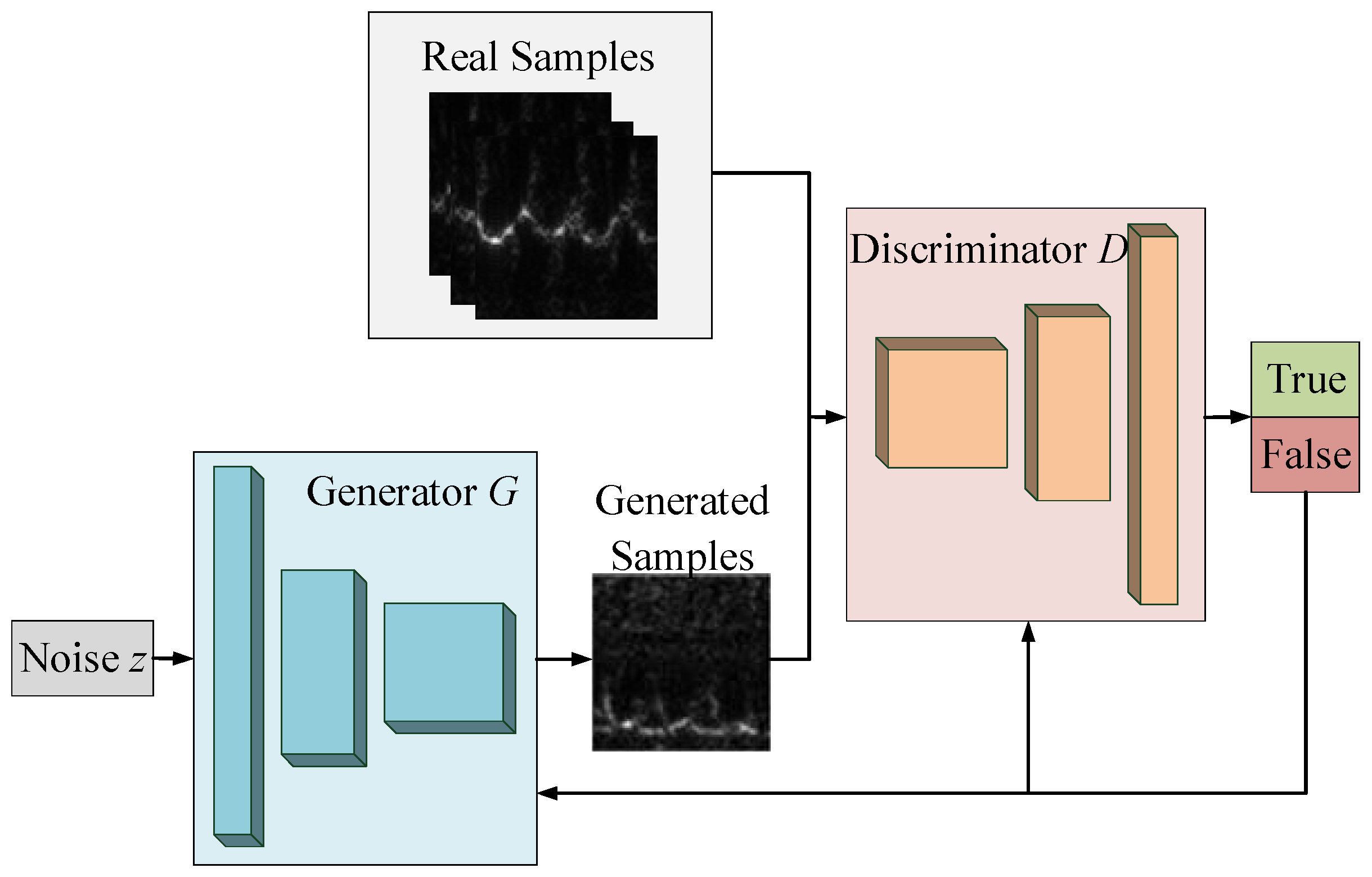
Inspired by the zero-sum game between two people, Goodfellow et al. [30] proposed the GAN structure. It consists of a generator and a discriminator. The generator is used to capture the distribution model of the time–frequency spectrogram of real ground moving targets and to generate new data samples. The discriminator is a binary classifier that determines whether the network input is real or generated data. The generator and discriminator iteratively optimize their parameters by competing and restricting each other to improve their abilities to generate and discriminate samples. In fact, this optimization process represents a game problem, which is to find an equilibrium point between the generator and discriminator. If the Nash equilibrium is reached, the discriminator cannot determine whether the input data come from the generator or denote real samples, and that is when the generator reaches the optimum state.
The structure of GAN is shown in Figure 1. The input of the generator is a one-dimensional random Gaussian noise vector z , and its output is a spurious time–frequency spectrogram G ( z ) . The input of the discriminator is the spectrogram sample G ( z ) of a ground moving target or a spectrogram sample generated by the generator, and its output is either “1” or “0,” where “1” represents true and “0” represents false. The training goal of the GAN is to make the distribution of the spurious spectrogram G ( z ) generated by the generator as close as possible to that of the real target. The purpose of the generator is to make the distribution of the generated spurious spectrogram on the discriminator D [ G ( z ) ] as consistent as possible with that of the real target D [ x ] . The loss function of the generator is given by:
min G V G ( D , G ) = min G { E z ~ p z [ log ( 1 D [ G ( z ) ] ) ] } ,
where D indicates the discriminator; G indicates the generator; p z is the random noise distribution; E ( ) is the expectation operator.
In the process of constant confrontation learning, a spurious time–frequency image generated by the generator G ( z ) becomes more close to the real time–frequency image of a ground moving target, and the discriminator becomes more fuzzy for G ( z ) .
The purpose of the discriminator is to realize the binary classification of input images. If the input is a real spectrogram sample, the discriminator will output “1”; but if the input is a spurious spectrogram generated by the generator G ( z ) , the discriminator will output “0.” The loss function of the discriminator is given by:
max D V D ( D , G ) = max G { E x ~ p d a t a [ log ( D ( x ) ) ] + E z ~ p z [ log ( 1 D [ G ( z ) ] ) ] } .
Thus, the total loss function of the generator and discriminator can be expressed as follows:
min G max D V D ( D , G ) = min G max G { E x ~ p d a t a [ log ( D ( x ) ) ] + E z ~ p z [ log ( 1 D [ G ( z ) ] ) ] } ,
where p d a t a is the time–frequency spectrum distribution of real targets.
However, the GAN has the problem of instability in the training process. Particularly, in the case when the discriminator does not converge well, the generator cannot be updated many times; otherwise, it will be prone to mode collapse.
A deep convolutional GAN (DCGAN) introduces a series of constraints to the original GAN structure. The DCGAN mainly improves the GAN from the engineering point of view, improving the stability of GAN training. Although there is not much innovation in this theory, it provides engineering support for the GAN development.
The main changes in the DCGAN structure compared to the ordinary GAN structure can be summarized as follows:
(1) The pooling and fully connected layers are removed from the discriminator, and a fully convoluted network is used to map the input sample to a two-dimensional vector to reduce the network parameters.
(2) In the generator, the transposed convolution layer is used to map the input random Gaussian noise vector to generate samples.
(3) To stabilize the training and convergence of the network, batch processing is used to normalize the convolution and transposed convolution layers.
(4) In the generator, the output layer uses the hyperbolic tangent function (tanh) as an activation function, while the other layers use the ReLu activation function after batch normalization.
(5) In the discriminator, to prevent the problem of gradient dispersion when the loss function of the discriminant network propagates to the generated network, the ReLU activation function is replaced by the leaky ReLU activation function so that the negative value input also has an activation output.
The structure of the generated DCGAN network is shown in Figure 2, where the input noise vector has a dimension of 100, and the output sample with a dimension of [3,64,64] is obtained through the transposed convolution with a step size of two in four layers. Although the DCGAN has an efficient network architecture, which can improve the stability of training to a certain extent, there is still the problems of unstable training, mode collapse, and inability to indicate the training process. To overcome these problems, this paper proposes a WGAN, which represents an improved DCGAN structure. The specific principle and improvement of WGAN will be described below.

3. GMT-WGAN for Target Classification

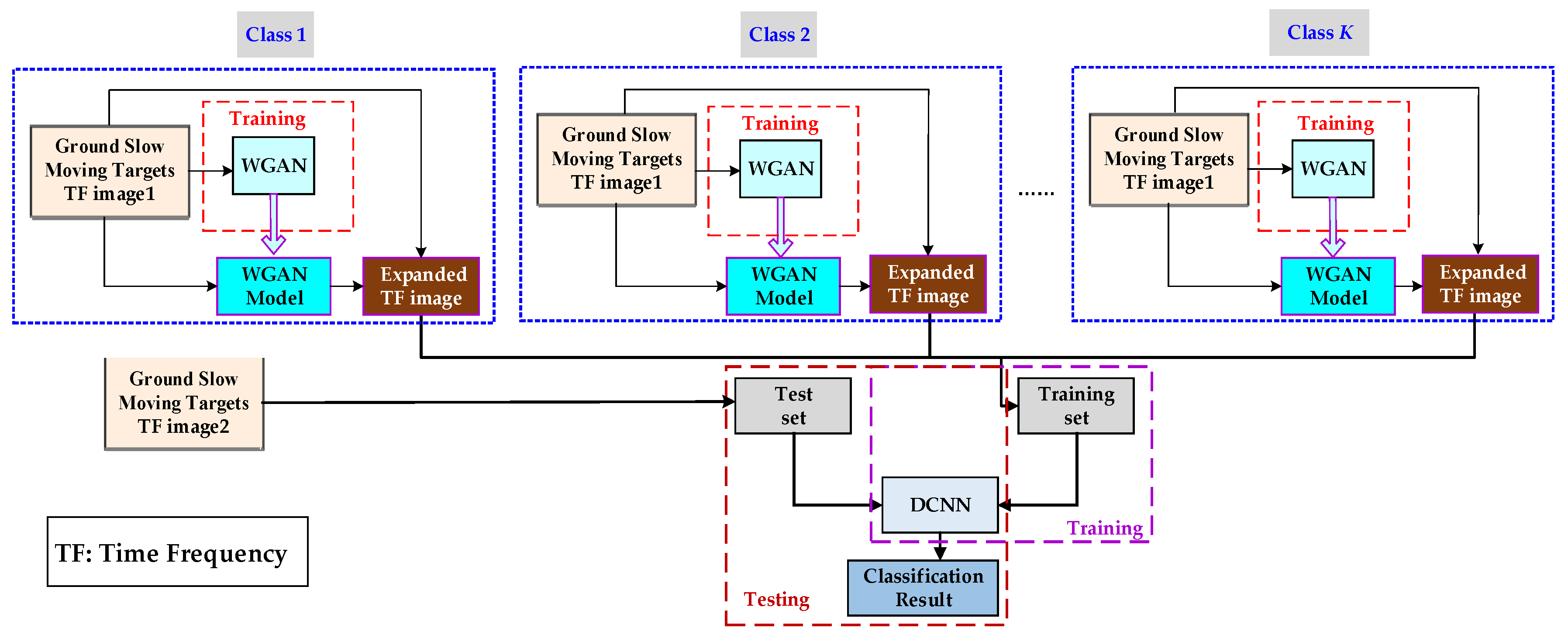
The flowchart of the proposed GMT-WGAN classification method is presented in Figure 3. The original time–frequency images of the ground moving targets are divided into two parts. The first part is used to train the WGAN. In the training process, through countermeasures between the generator and discriminator, the Nash equilibrium is achieved, a well-trained WGAN model is obtained, and the time–frequency images of ground moving targets are generated. Then, the generated time–frequency images and the first part of the original time–frequency images are mixed to form the DCNN training set, which is fed to the DCNN to train the network parameters and learn the inherent characteristics of time–frequency images until convergence. Finally, the second part of the original time–frequency images is used as the DCNN test set, which is fed to the trained DCNN, and outputs the classification labels to achieve the robust classification of ground moving targets. The specific principles are introduced in detail below.

3.1. Data Expansion Method Based on WGAN

Although common deep-learning-based methods can achieve good classification results, they require a large number of training and testing samples. If there are fewer samples, the overfitting phenomenon can appear, resulting in a poor classification effect. Therefore, it is necessary to enhance and augment data samples. Most traditional image transformation methods are global and can neither focus on the diversity of local regions nor extract the intrinsic features of a database. To alleviate these drawbacks, this paper proposes a data enhancement method based on the WGAN.
The GAN and DCGAN structures have certain problems, such as difficulty in training and the loss function of generator and discriminator cannot indicate the training process and mode collapse. The Jensen–Shannon (JS) divergence (the first form) and Kullback–Leibler (KL) divergence (the second form) are used by the GAN to calculate the distance between the generated and real distributions. When the JS divergence is used, if the intersection of two distributions is very small or in a low-dimensional manifold space, then the discriminator D can easily find a discriminant surface to distinguish the generated distribution from the real distribution. Therefore, it cannot provide effective gradient information to the generator in the backpropagation process. In other words, the loss function is not continuous. Due to the ineffective gradient information, network parameters of the generator G cannot be effectively updated, which makes training difficult. Since the KL divergence is asymmetric, the generator tends to generate samples that are easier to pass through, which makes it easier to cause a mode crash. In addition, there is no single indicator that can measure the status of network training.
The WGAN introduces Wasserstein distance to measure the difference between two distributions. Wasserstein distance, which is also known as the earth-mover distance, is defined as follows [35]:
W ( P r , P g ) = inf γ ~ ( P r , P g ) E ( x , y ) ~ γ [ x y ] ,
where ( P r , P g ) represents the set of all possible joint distributions of distributions P r and P g .
For each possible joint distribution γ , a real sample x and a generated sample y can be sampled from ( x , y ) ~ γ , and the distance between the samples x y can be calculated. Therefore, the expected value E ( x , y ) ~ γ [ x y ] of the sample distance under the joint distribution γ can be calculated. In all possible joint distributions, the lower bound of the expected value is inf γ ~ ( P r , P g ) E ( x , y ) ~ γ [ x y ] , and it is also defined as Wasserstein distance. Intuitively, this can be understood as the “consumption” needed to move the pile of “sand” P r to P g under the “path planning” γ , which gives it the name of earth-mover distance, where W ( P r , P g ) is the minimum consumption under the optimal path planning. Wasserstein has a better distance measure than any other divergence. This is because Wasserstein distance measures the distance between two distributions, even if they show almost no overlapping. This advantage enables the WGAN to alleviate gradient dispersion in the process of GAN training. In particular, the discriminator D can still propagate effective gradient to the generator G when two distributions almost do not overlap. In practice, mathematical transformations have been commonly used to express the Wasserstein distance in a solvable form, and the weight of the discriminator is maximized by using weight clipping to limit it within a range so as to approximate the Wasserstein distance. By using this approximate optimal discriminator, the optimization generator increases the Wasserstein distance, thus effectively shortening the distance between the generated and real distributions. The network structure of the discriminator of the proposed WGAN is presented in Figure 4.
The main contribution of the WGAN is that instead of using the JS or KL divergence, the Wasserstein distance is used to measure the difference between the real and generated data distributions. Compared with the JS divergence, the Wasserstein distance is continuous, which makes the discriminator loss be no longer defined by binary values (true or false), and transforms it into a regression problem. At the same time, due to the continuity of the loss function and weight cutting, the training is more stable. Compared with the KL divergence, the Wasserstein distance is symmetric, and the generator training has a stable tendency, so the mode crash problem is overcome. Finally, since the GAN cannot generate indicators, which indicate the training process, the Wasserstein distance is the inverse of the discriminator loss function, so the difference between the real and generated distributions can be obtained by the discriminator loss function. The Wasserstein distance does not depend on the discriminator’s network structure, can indicate the training process, and is highly correlated with the quality of generated samples. In conclusion, the advantages of the WGAN can be summarized as follows:
(1) It solves the problems of unstable GAN training and the requirement for balancing the training degree of the generator and discriminator.
(2) It solves the problem of a mode crash and ensures the diversity of generated samples.
(3) In the training process, it generates a value that can indicate the training process state (i.e., the inverse of the discriminator loss function). The smaller this value is, the better the GAN’s training performance and the higher the image quality will be.

3.2. DCNN-Based Ground Moving Target Classification

In this study, a VGG-16 network is used to classify ground moving targets. The VGG-16 network structure is shown in Figure 5. Input samples of the VGG-16 are grayscale images or RGB images labeled in the one-hot form. The VGG-16 network consists of five convolutional blocks and one fully connected block. The convolution block includes two or three convolution layers, each of which has the extracted feature map depth of m and the convolution kernel size of n × n ; thus, the convolution of this type of layer is denoted as m @ n × n . After the convolution layers, the ReLU function is used to activate and transfer the feature map to the pooling layer. The window size of the maximum pooling layer is 2 × 2. After the convolutional block, the feature map is reconstructed into a one-dimensional feature vector by the fully connected layers. Finally, the softmax layer maps the vector into probability values to obtain the category and calculate the classification accuracy. The parameters of the network layers are shown in Figure 5.

3.3. Image Quality Evaluation Metrics

Although the generated images can augment and enrich the sample database, if the quality of generated images is not high enough, or there exists a large difference between generated and original images, adding the generated images will not help to improve the performance but instead will decrease the classification accuracy. Therefore, the quality of generated images needs to be evaluated.
The common image quality evaluation indexes include mean value, entropy, dynamic region, fuzzy linear index, mean gradient, mean variance, and gray difference. The evaluation metrics are introduced in the following.
  • Mean value
The mean of an image indicates its total energy. Assume the size of an image I is M × N ; then, the mean value of the image is given by:
Mean = 1 M N m = 1 M n = 1 N I ( m , n ) .
  • Variance
The variance of an image indicates the deviation degree of the image relative to the mean value, which can be expressed as follows:
Variance = 1 M N m = 1 M n = 1 N ( I ( m , n ) Mean ) 2 .
  • Information entropy
Information entropy indicates the amount of information in an image and reflects the degree of focus of the image. The information entropy is calculated by:
H = i = 1 M j = 1 N p i j log p i j ,
where p i j is the probability value of pixels in image I ( i , j ) .
The smaller the information entropy value is, the more focused the image is.
  • Dynamic zone
The dynamic zone denotes a ratio of the maximum value to the minimum value of a grayscale image, and its logarithmic expression is as follows:
D = 10 log I max I min ,
where I max and I min denote the maximum and minimum values of the grayscale image, respectively.
The larger the dynamic range is, the higher the image contrast is.
  • Linear index of fuzziness
The linear index of fuzziness (LIF) is used to describe the fuzzy degree of an image, and it is defined by:
LIF = 2 M N m = 1 M n = 1 N min [ p m n , ( 1 p m n ) ] ,
p m n = sin { π 2 × [ 1 I ( m , n ) I max ] } .
The smaller the LIF value is, the sharper the image is.
  • Average gradient
The average gradient (AG) of an image is calculated by:
AG = 1 ( M 1 ) ( N 1 ) m = 1 M 1 n = 1 N 1 1 4 [ I ( m , n ) m ] 2 + [ I ( m , n ) n ] 2 ,
where I / m and I / n represent the horizontal and vertical gradients of the image, respectively.
The larger the AG value is, the clearer the edge details of the image are.
  • Gray level difference
The gray level difference (GLD) of an image indicates the edge sharpness of the target area of interest in the image, and it is obtained by:
GLD = 1 ( M 1 ) ( N 1 ) m = 1 M 1 n 1 N 1 | I ( m , n ) I ( m + 1 , n ) | + | I ( m , n ) I ( m , n + 1 ) | .
The larger the GLD value is, the clearer the image edge is.
4. Experiments

4.1. Construction of Ground Moving Target Data

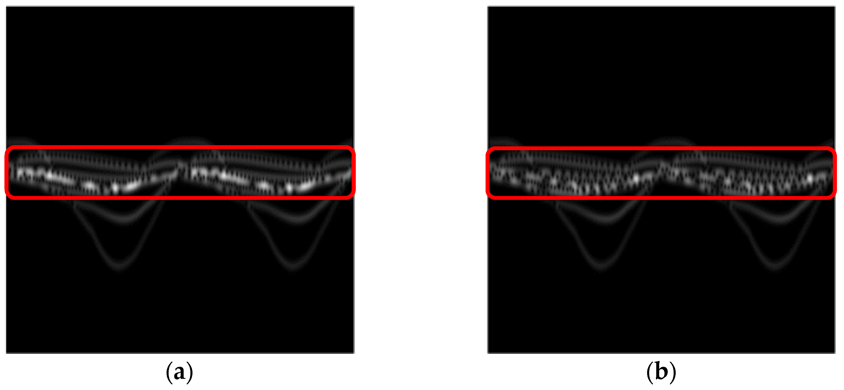
4.1.1. Pedestrian Armed and Unarmed Simulation Data

The movement mechanism of pedestrians is very complex. During the movement, the parts of the human body are highly coordinated and mutually constrained. Fortunately, V. C. Chen [6] provided a research foundation for pedestrian motion simulations. The Boulic model proposed in [6] can describe the pedestrian model at different walking speeds only in the normal walking mode. Still, based on this method, the movement state of an armed pedestrian can be obtained by introducing certain modifications. The upper and lower arms of the pedestrian are vertical, moving forward and vibrating up and down with the torso, while their position relative to the center of gravity of the torso remains unchanged, which can be used to describe the motion posture of the armed walking. The unarmed state is the type of normal walking. By changing the heights and relative movement speeds of pedestrians, this study constructs a database of armed and unarmed pedestrian walking. The specific simulation parameters used for constructing the database are given in Table 1.
Figure 6 shows the time–frequency spectrograms of a pedestrian when it is armed and unarmed. Figure 6a displays the time–frequency spectrogram of the unarmed pedestrian normal walking, and Figure 6b presents the time–frequency spectrogram of the armed pedestrian walking. Compared with Figure 6b, the swing of a pedestrian’s arms during normal walking can be clearly distinguished from the red box in Figure 6a.

4.1.2. Semi-Measured Pedestrian Posture Data Based on MOCAP

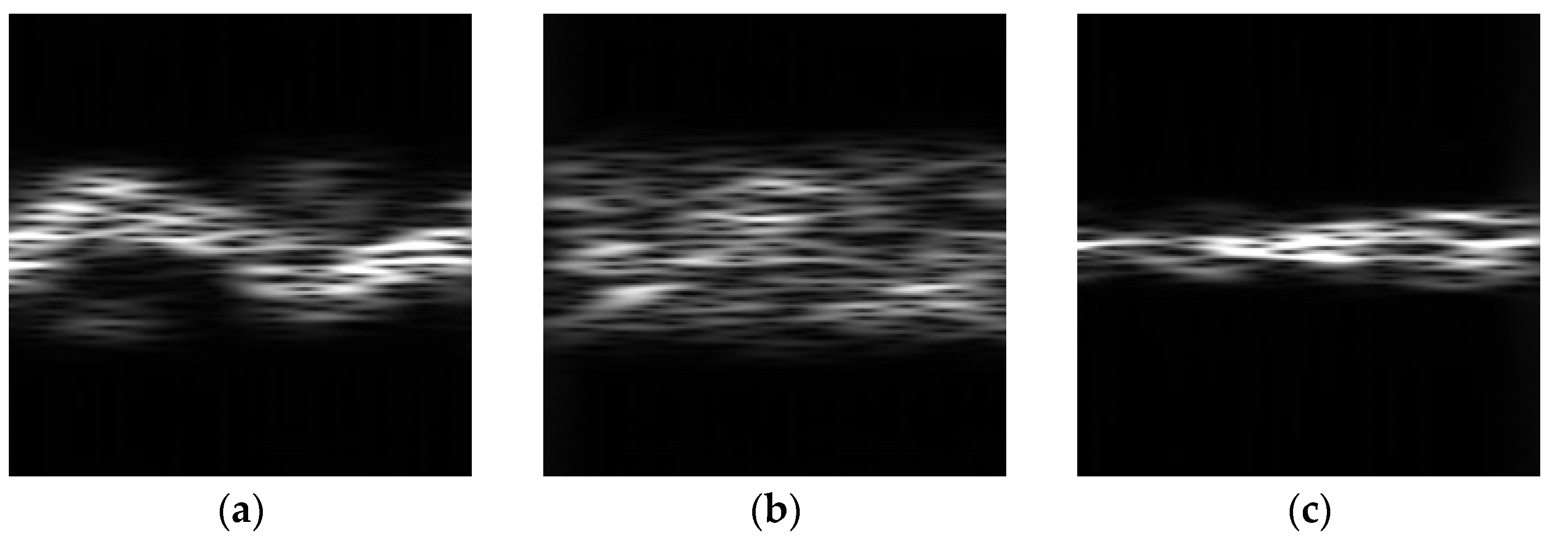
Since the measured radar echo signals of pedestrians are difficult to obtain, this study uses the MOCAP data disclosed by Carnegie Mellon University to approximate the motion of various parts of a pedestrian body and the physical optics method to describe their electromagnetic (EM) properties [41]. The MOCAP data treat the three-dimensional human body as a collection of rigid bodies connected by joint points and represents each body part as a line segment, thereby simplifying the pedestrian movement to the movement of a human skeleton frame. Using the hierarchical recursion relationship, the motion trajectories of different parts of a pedestrian body at different moments can be calculated. At the same time, the pedestrian body parts are modeled as ellipsoids according to the length of each part obtained from the MOCAP data. Based on the motion trajectory of each part of a pedestrian body, the relationship between the pedestrian and radar is updated in real-time. The physical optics method is used to calculate the total RCS of a pedestrian at each moment in real-time, thus constructing the radar echo signal of the pedestrian. The MOCAP data contain a variety of pedestrian movements, which can be batch-processed to obtain a database of radar echo signals with different postures of pedestrians. It should be noted that this study analyzes only three common movement postures, namely, walking, running, and jumping. The simulation parameters were set as follows. A bistatic radar, which transmits a single frequency signal with a carrier frequency of 35 GHz, was used. The pitch angle of the EM wave of the transmitting antenna was 87.7° and the azimuth angle was 210.17°. The pitch angle of the EM wave of the receiving antenna was 87.7° and the azimuth angle was 149.83°. Thus, the double base angle was about 60°. After calculation and time–frequency transformation, 16 walking samples, 8 running samples, and 9 jumping samples were obtained. The samples were all grayscale time–frequency spectrograms with a size of 2048 × 512.
The time–frequency spectrograms of the echo signals for different pedestrian postures are presented in Figure 7. Figure 7a shows the time–frequency spectrogram of the walking posture, where the acceleration/deceleration process of the pedestrian torso and the periodicity of the movement can be clearly observed. Figure 7b displays the time–frequency spectrogram of the running posture. Since the admission time was too short, a clear periodic curve cannot be clearly observed in Figure 7b, but it can be noticed that the time–frequency information of each part in the running posture is more abundant than that of the walking posture. Figure 7c shows the time–frequency spectrogram of the jumping posture, including the walking and take-off process of the pedestrian. In Figure 7, it can be observed that the time–frequency spectrograms of the three postures have different micro-motion characteristics. Therefore, they can be classified and identified according to their time–frequency spectrograms.

4.1.3. Measured Ground Moving Target Data

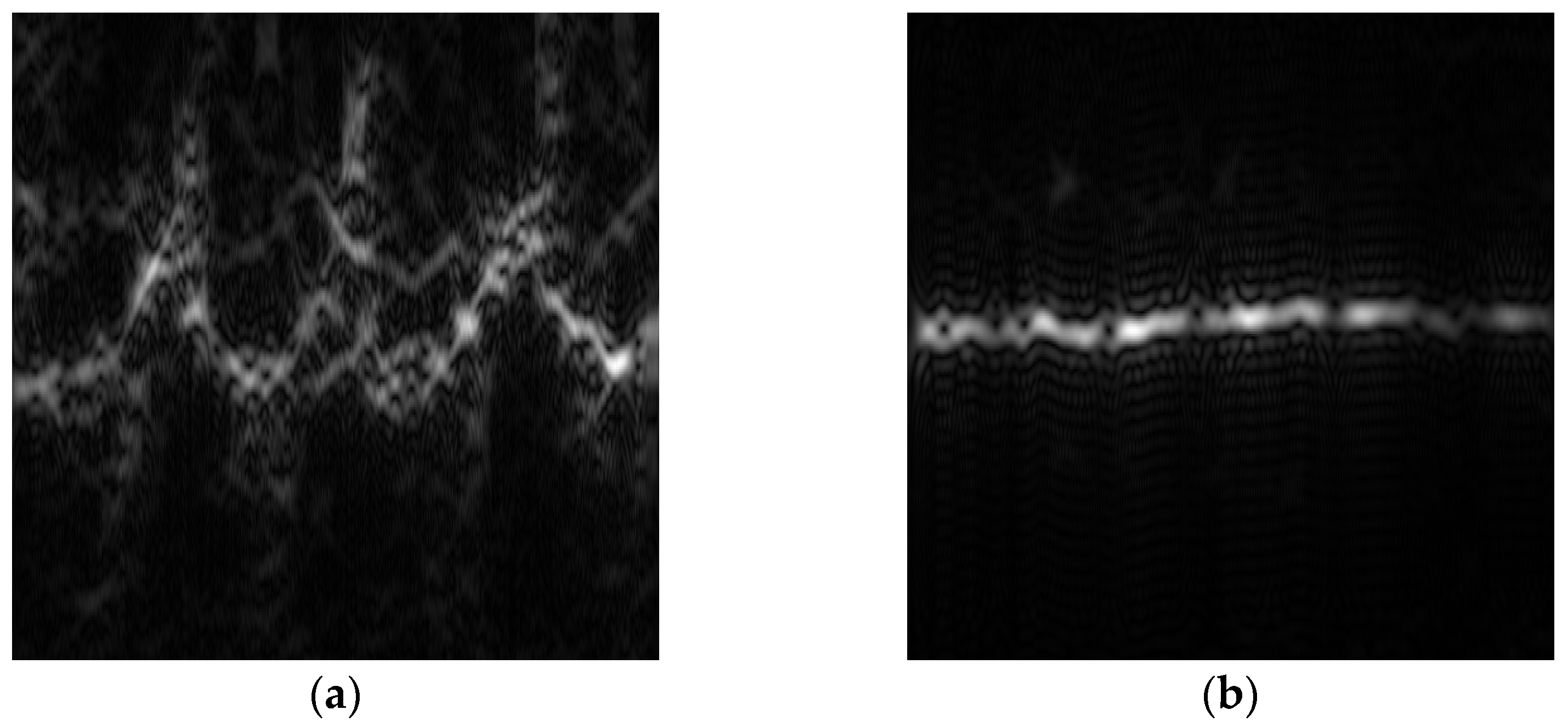
To verify the performance of the proposed method in practical applications, this paper used the measured data of pedestrian and vehicle targets for verification. During the data collection process, the radar transmitted a narrow-band linear frequency-modulated continuous wave (LFMCW) signal and received the beat signal. The specific experimental parameters are given in Table 2. To enrich the dataset, all collected data samples were preprocessed using a time sliding window, and 351 time–frequency spectrograms were obtained, of which 128 were spectrograms of pedestrians and the other 173 spectrograms related to vehicles.
The time–frequency spectrograms of the measured data of pedestrians and vehicles are presented in Figure 8. Figure 8a shows the spectrogram of the pedestrian movement, where the periodicity of the pedestrian movement, the swing of limbs, and the acceleration/deceleration process of the torso can be clearly observed. Figure 8b displays the time–frequency spectrogram of a wheeled vehicle. Since the micro-motion of a wheeled vehicle mainly depends on the rotation of a tire, which is made of rubber, the RCS was smaller than that of the vehicle body. Therefore, in Figure 8b, the micro-Doppler component is almost invisible in the time–frequency spectrogram, while the frequency component of the vehicle body in Figure 8a is dominant. By comparing Figure 8a,b, significant differences in the time–frequency domain can be observed. Therefore, these two types of targets can be classified based on their time–frequency spectrograms.

4.2. Ground Moving Target Data Expansion and Performance Analysis

4.2.1. Data Expansion

Due to the limited amount of training data, it is impossible to extract a large number of statistical features or general descriptions of features or conduct effective training of a deep learning model. Therefore, the WGAN is used to augment the constructed databases.
In this study, three databases were used: (1) an armed and unarmed pedestrian simulation database obtained using a modified Boulic model; (2) a semi-measured pedestrian posture database obtained from MOCAP and EM data; (3) a pedestrian and vehicle target database obtained from the measured data. The network parameters are shown in Table 3.
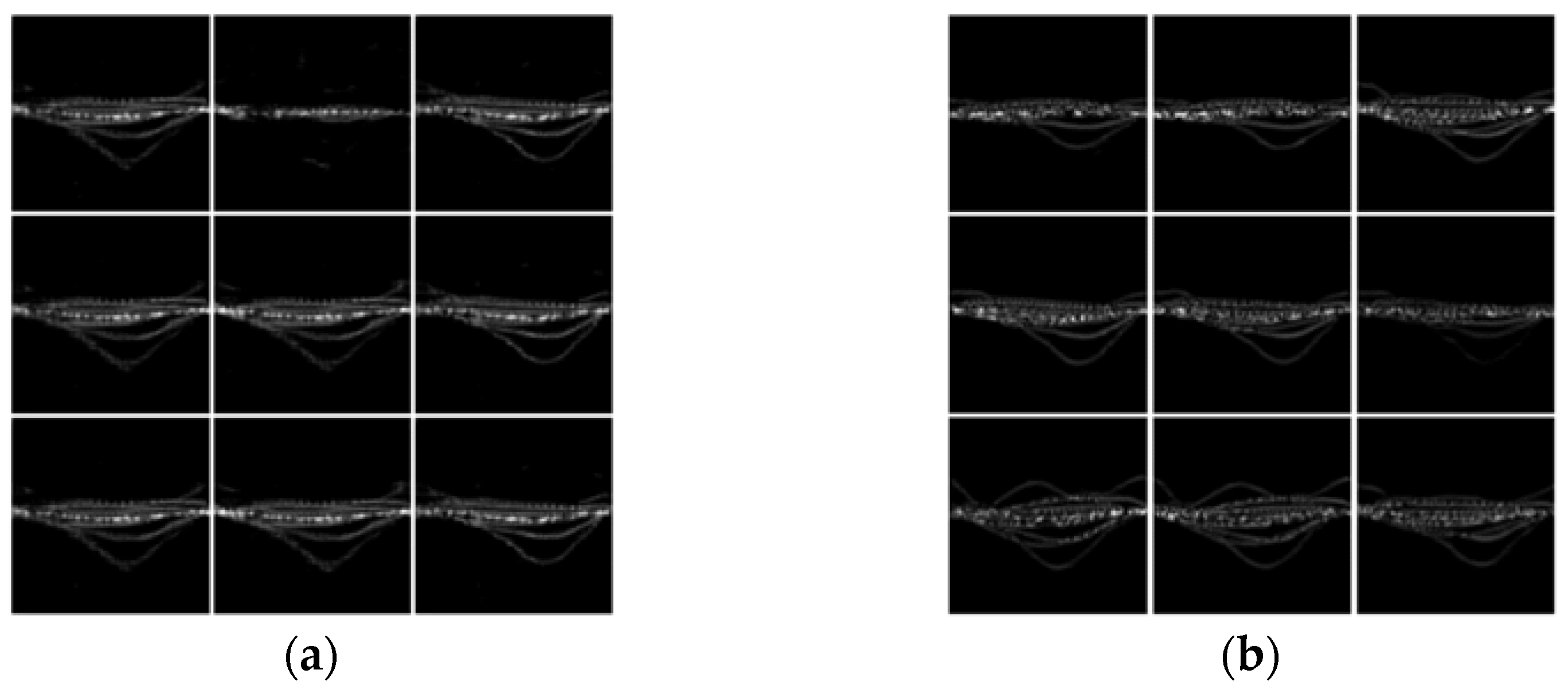
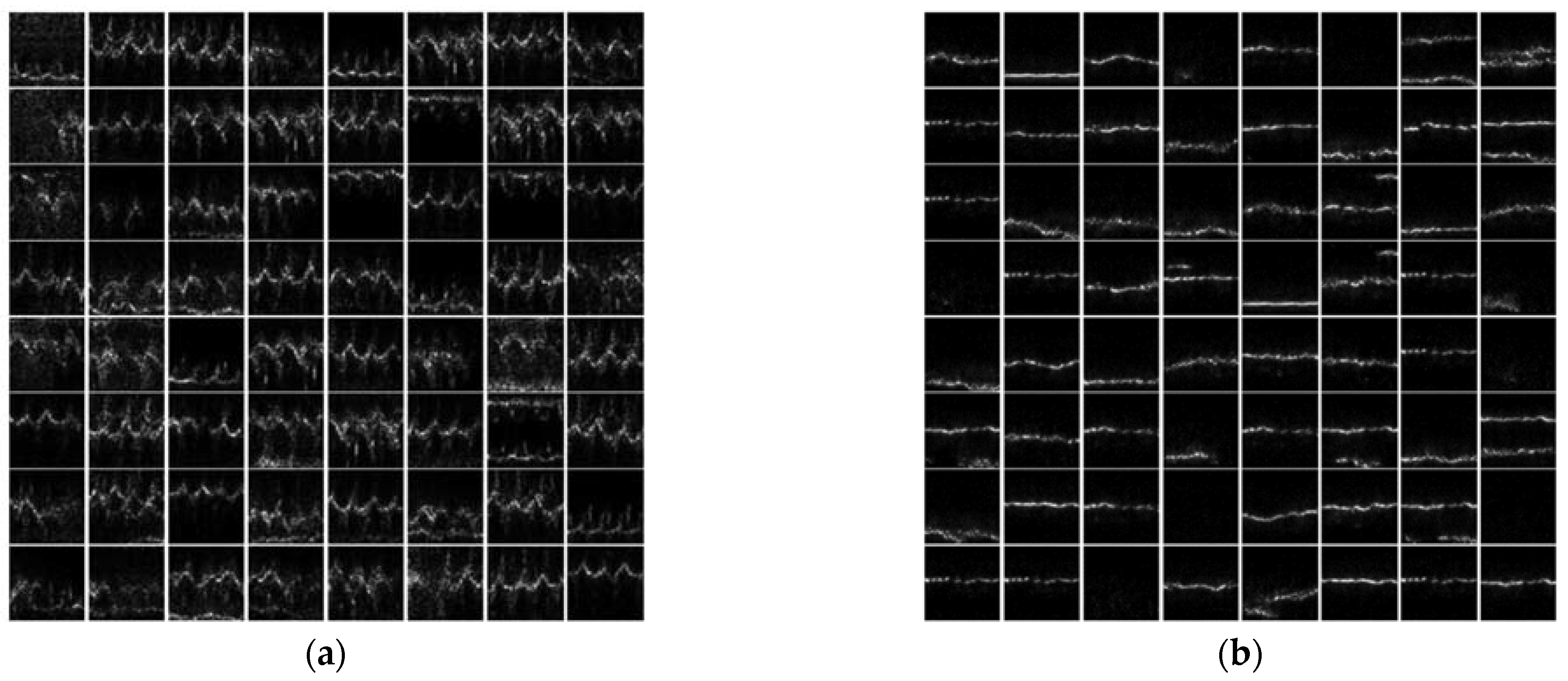
When the confrontation learning of the generator and discriminator converges, the noise vector is fed to the generator, and the generated distribution can be sampled to obtain the generated samples. For the three databases, the generated samples are shown in Figure 9, Figure 10 and Figure 11, and it can be seen that the generated samples are close to the data distribution of real samples to a certain extent. In addition, the generated samples are diversified, which indicates that the WGAN has captured the inherent characteristics of real samples.

4.2.2. Evaluation of Generated Samples

In this study, seven statistical and evaluation indexes were used to evaluate the effectiveness of generated samples obtained by the generator. The physical meaning of each of them is given in Section 3.3. The specific evaluation method was as follows. For each database, the statistical evaluation indexes of the real and generated samples were calculated and used to evaluate the data distribution similarity between the generated and real samples. The closer the evaluation indexes were, the higher the data distribution similarity was. Moreover, in order to compare the differences between WGAN generating samples and ordinary GAN generating samples, this section also calculates the evaluation metrics of GAN-generating samples.
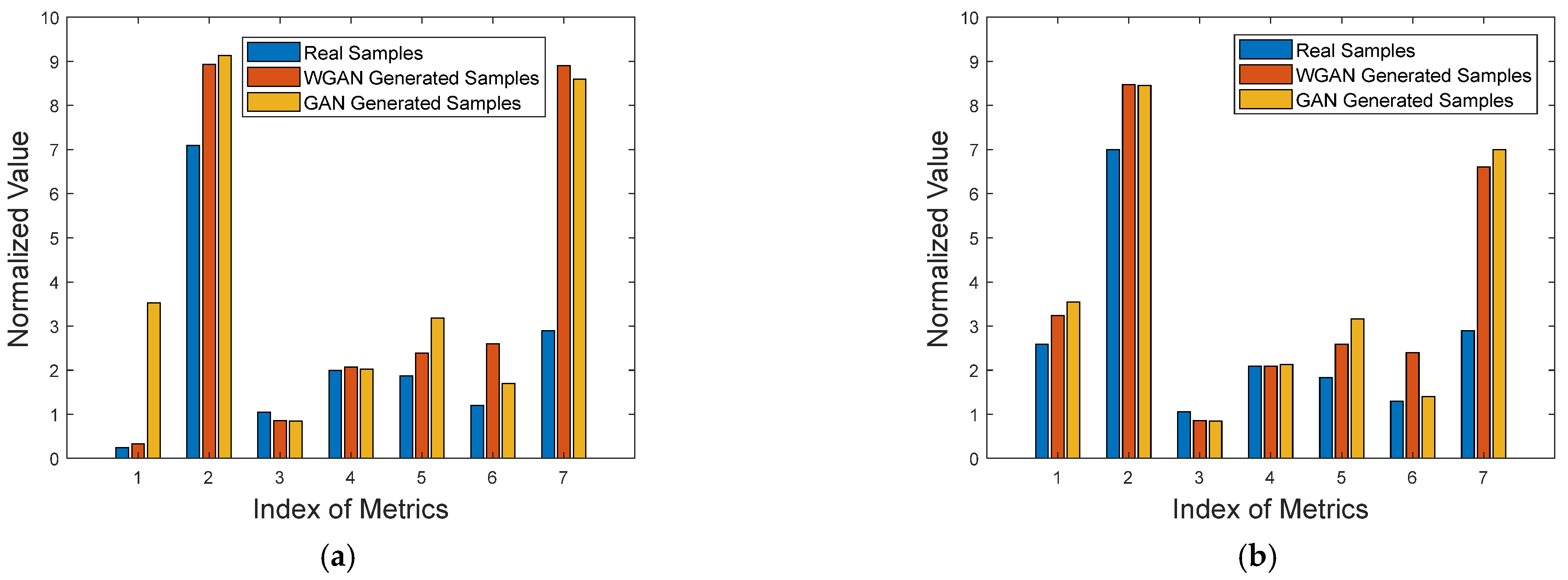
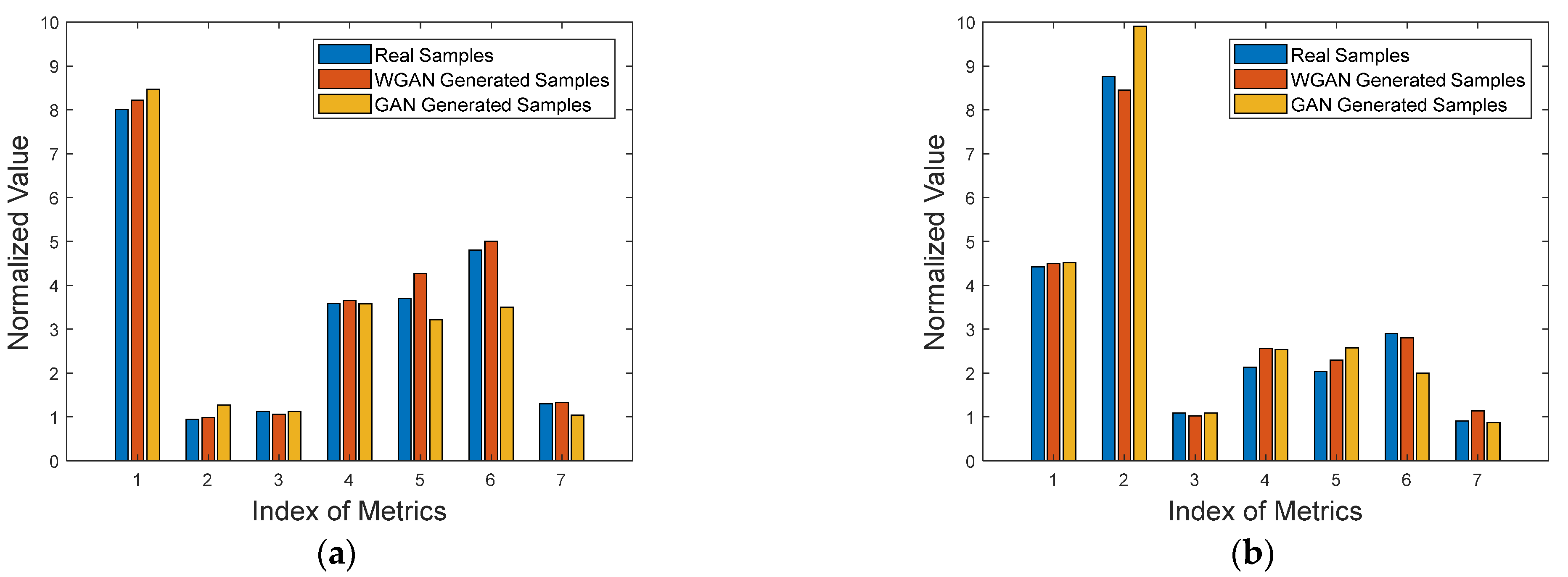
The evaluation index values of generated samples of the database obtained using the modified Boulic model are shown in Table 4. This database contained two sample categories related to unarmed and armed pedestrians. To analyze the distribution differences between the generated and real samples intuitively, the values of the evaluation metrics were normalized and limited to the range of 0–10, as presented in Figure 12, where the horizontal axis denotes the indexes: “1” denotes the mean value, “2” denotes the variance, “3” represents the entropy, “4” stands for the dynamic zone, “5” expresses the LIF value, “6” indicates the AG value, and “7” denotes the GLD value. This presentation has been adopted because the calculated metrics were distributed in different numerical ranges. The vertical axis in Figure 12 denotes the normalized value of the metrics. As shown in Figure 12, for both armed and unarmed pedestrians, all metrics of the generated samples except for the entropy were slightly higher than those of the real samples, while the degrees of differences were similar. Furthermore, the metrics with the largest difference in distribution between the two types of samples were AG and GLD. The AG value of the generated samples was higher than that of the real samples, which indicated that the edge details of the generated samples were clearer than those of the real samples. The GLD value of the generated samples was higher than that of the real samples, indicating that the main components of the generated images contained more high-frequency information than the real images. Based on these two metrics, the generated samples had sharper image edges than the real data samples. In addition, there is little difference between the metrics of the samples generated by WGAN and ordinary GAN. Only the LIF of WGAN samples is slightly lower than that of GAN samples, and the AG of WGAN samples is slightly higher than that of GAN samples, indicating that the edge details of the samples generated by WGAN are clearer.
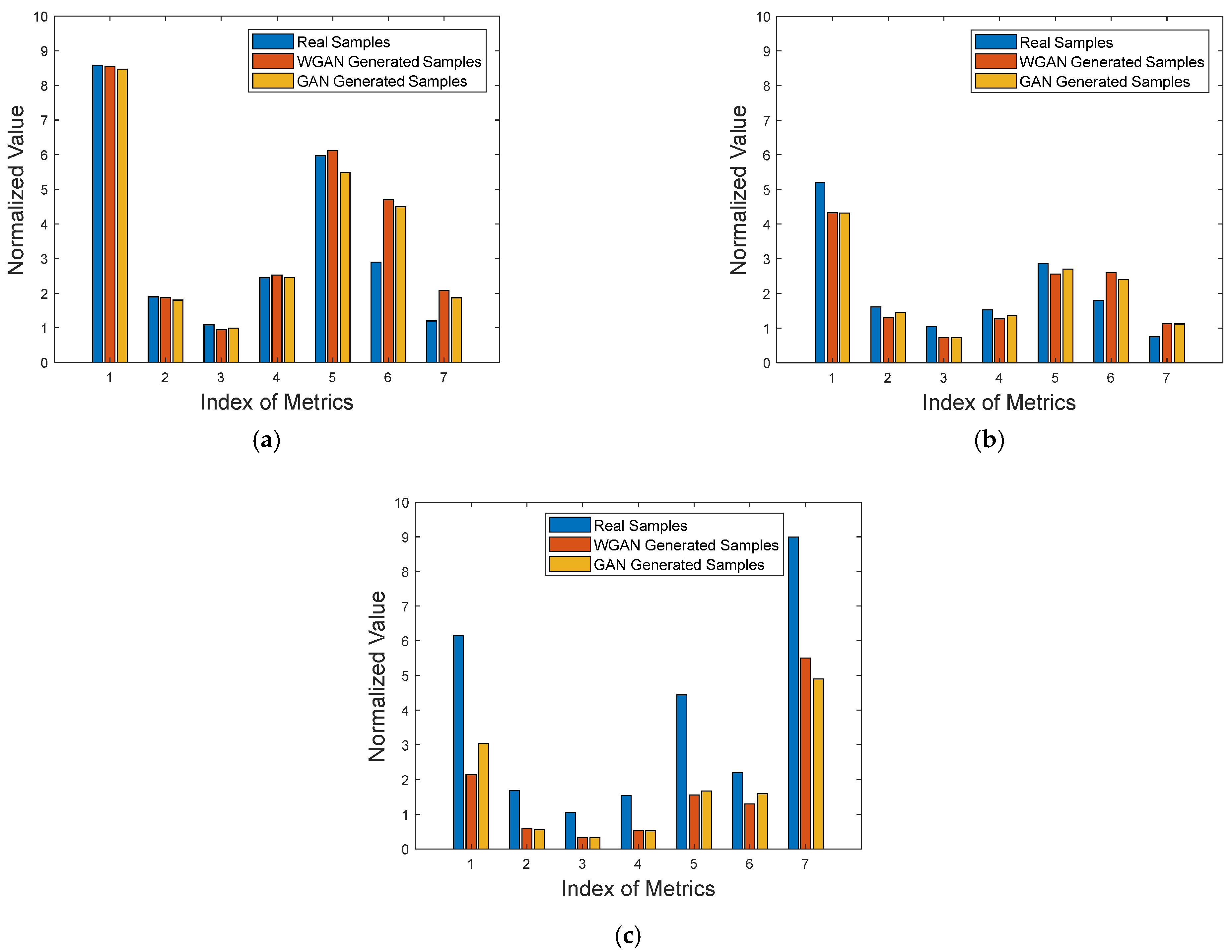
The evaluation metric values of the generated samples from the database obtained from the MOCAP and EM data, which includes walking, jumping, and running samples, are given in Table 5. Similarly, the normalized values of these metrics are shown in Figure 13. The results show that for walking samples, there was a slight difference in the distribution of the first five metrics between real and generated samples, while the values of the AG and GLD metrics of the generated samples were higher than those of the real samples, indicating that the generated samples had clearer image edges than the real samples. For jumping samples, where the number of real samples was fewer, in addition to the difference in the AG and GLD metrics, there were also obvious differences in the values of the first five metrics; namely, the metric values of the generated samples were slightly lower than those of the real samples. For the running samples, the number of real samples was smaller than that of the walking samples, and the generator of the WGAN could achieve the balance of data distribution earlier, so the distribution of the generated samples was different from that of the real samples. For the two GAN-based methods, the difference between the generated samples of WGAN and ordinary GAN is very small, indicating that the advantages of WGAN are not obvious under this sample.
The evaluation metric values of the generated samples from the database obtained from the measured data, which consisted of both pedestrian and vehicle samples, are shown in Table 6. Similarly, the normalized values of the metrics are shown in Figure 14. Based on the results, for the two types of samples, the distributions of real and generated samples from WGAN were very close due to the large number of samples, which validated the effectiveness of the sample distribution learned by the WGAN generator. For the pedestrian samples, the variance of the generated samples from WGAN was slightly higher than that of the real samples, which indicated that the uniformity of numerical distribution of the generated samples was lower than that of the real samples. For the vehicle samples, the variance of the generated samples from WGAN was slightly lower than that of the real samples, indicating that the uniformity of numerical distribution of the generated samples from WGAN was higher than that of the real samples. Further, for the pedestrian samples, the AG value of the generated samples from WGAN was slightly higher than that of the real samples, which indicated that the edges of the generated samples were clearer than those of the real samples. For the vehicle samples, the AG value of the generated samples from WGAN was slightly lower than that of the real samples, indicating that the edges of the generated samples were blurrier than those of the real samples. For the two GAN-based methods, the generated samples of ordinary GAN are worse than those of WGAN, which shows that WGAN has obvious advantages when the sample details are rich, as the instability of ordinary GAN training leads to the poor quality of generated samples.
Based on the quantitative evaluation of the generated samples of the ground moving targets, the following conclusions can be drawn. (1) The effectiveness of generated samples is related to the number of real samples. When the number of real samples can meet the optimization requirements of the WGAN to a certain extent, the data distribution of generated samples can be close to that of real samples. (2) If the number of real samples is small, the generator can learn the data distribution effectively, but its AG and GLD values can be slightly higher than those of the real samples, indicating that the generated samples have clearer image edges than the real samples. (3) When the number of real samples is very small, including only a dozen samples, the WGAN network can still converge, but the generated samples will be quite different from the real samples, as well as the values of the metrics. However, considering that subsequent classification experiments have been conducted using the enhanced samples, the classification network structure is more sensitive to the spatial features of images. Therefore, in this case, the metric values of generated samples can be relatively different to those of real samples. On the contrary, the classification performance can be improved if generated samples have the spatial features of real samples.

4.3. Ground Moving Target Classification Based on Data Expansion and Performance Analysis

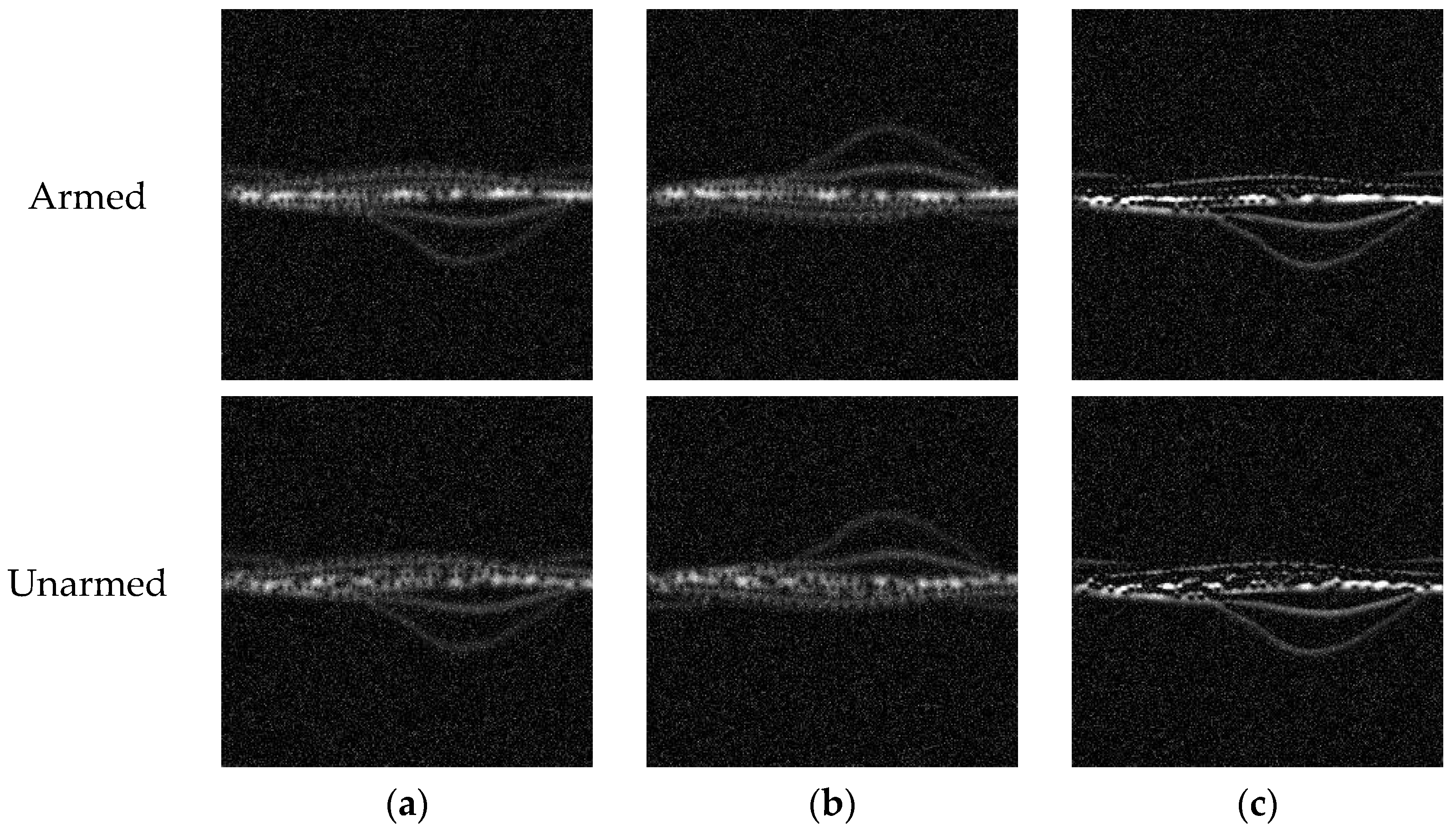
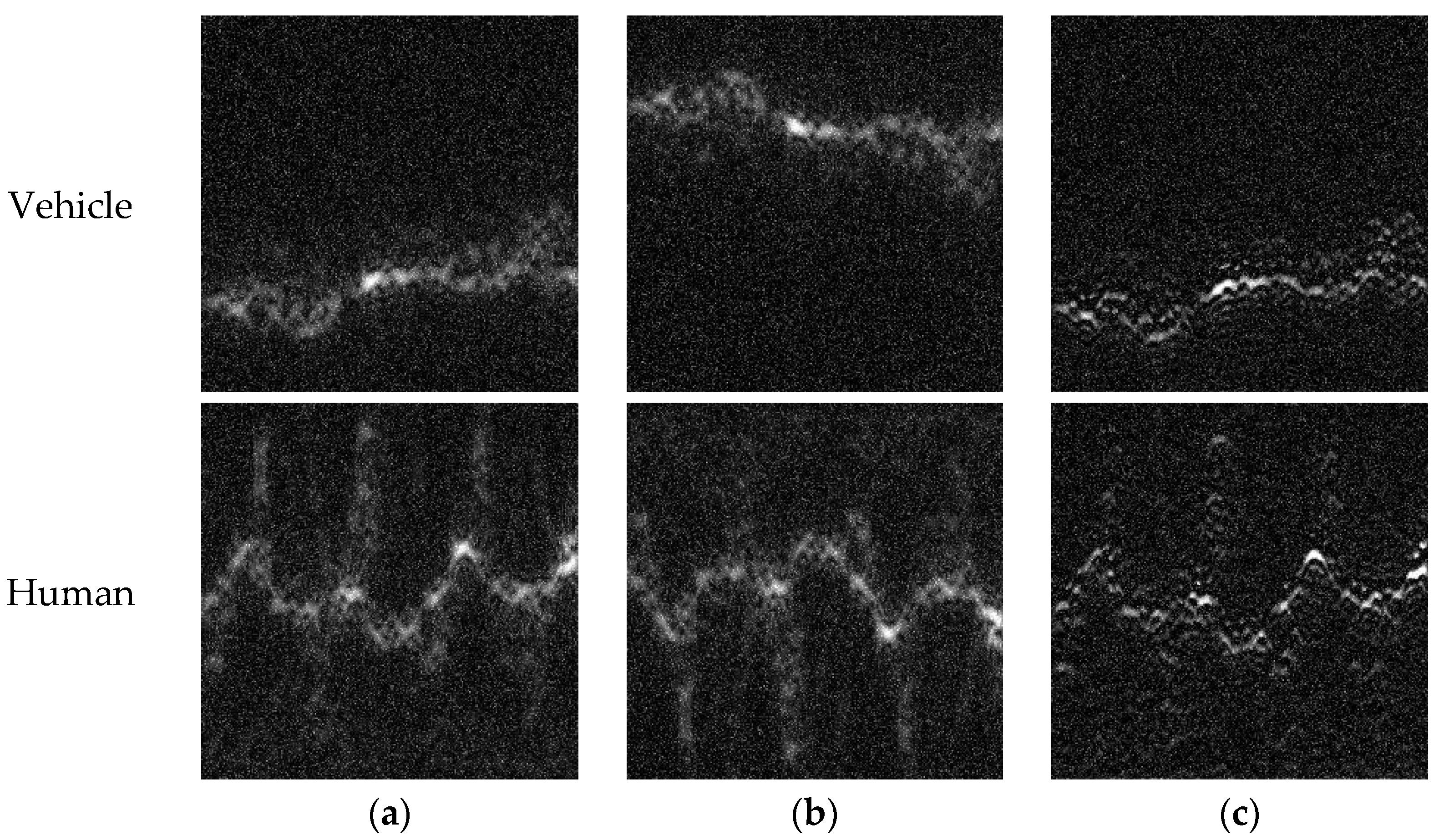
In previous experiments, the data of ground moving targets were enhanced, and a series of metrics were used to evaluate the effectiveness of generated samples quantitatively. In this section, the ground moving target samples before and after the data enhancement are classified, and the results of the contrast experiments conducted by different enhancement methods and noises to verify the performance improvement of the proposed method are presented. In these experiments, the traditional data enhancement methods of affine transformations [28] and image sharpening [29] were used. The images of the three databases obtained by the affine+sharpening method are shown in Figure 15, Figure 16 and Figure 17. Moreover, the ordinary GAN was also used for comparison with WGAN.
Figure 5 illustrates the structure of the classification network, whose input training samples belong to two categories: the original data that include real samples and augmented samples, which denote a mixture of real and generated samples. It is worth noticing that the generated samples were generated by three methods, namely, the WGAN, ordinary GAN and the affine+sharpening method.
The parameters of the classification network and dataset are given in Table 7. For the three databases of the ground moving targets, all of the input samples were gray images with a size of 256 × 256 . To verify the classification performance improvements achieved by the proposed sample enhancement method, the samples were separated into two parts. This first part included a randomly selected 10% of the original samples, which were used to train the WGAN, ordinary GAN and affine+sharpening method to obtain various generated samples. The second part included the remaining 90% of the data.
The experimental settings were as follows.
(1) The classification experiment performed using the original samples: Only 10% of the data were used to train the network, while the remaining data were used to test its performance.
(2) The classification experiment performed using the data enhanced by the WGAN: The training data represented a mixture of 10% of the original data and the WGAN-augmented data, while the remaining data were used as a test set.
(3) The classification experiment performed using the data enhanced by ordinary GAN method: The training data denoted a mixture of 10% of the original data and GAN-augmented samples, while the remaining data were used as a test set.
(4) The classification experiment performed using the data enhanced by theaffine+sharpening method: The training data denoted a mixture of 10% of the original data and affine+sharpening-augmented samples, while the remaining data were used as a test set.
The settings of the four experiments differed only in terms of the training set. Table 7 shows the parameters of the data samples before and after data enhancement. In this study, all methods augmented the real data by 50 times. The numbers of samples in the simulated, semi-measured, and measured datasets before data enhancement were 40, 12, and 34, and the numbers of generated samples were 2000, 600, and 1700, respectively. Further, the numbers of samples in the enhanced training sets of the simulated, semi-measured, and measured datasets were 2040, 612, and 1734, respectively, while the training sets after data enhancement by the WGAN, GAN, and affine+sharpening method were the same.
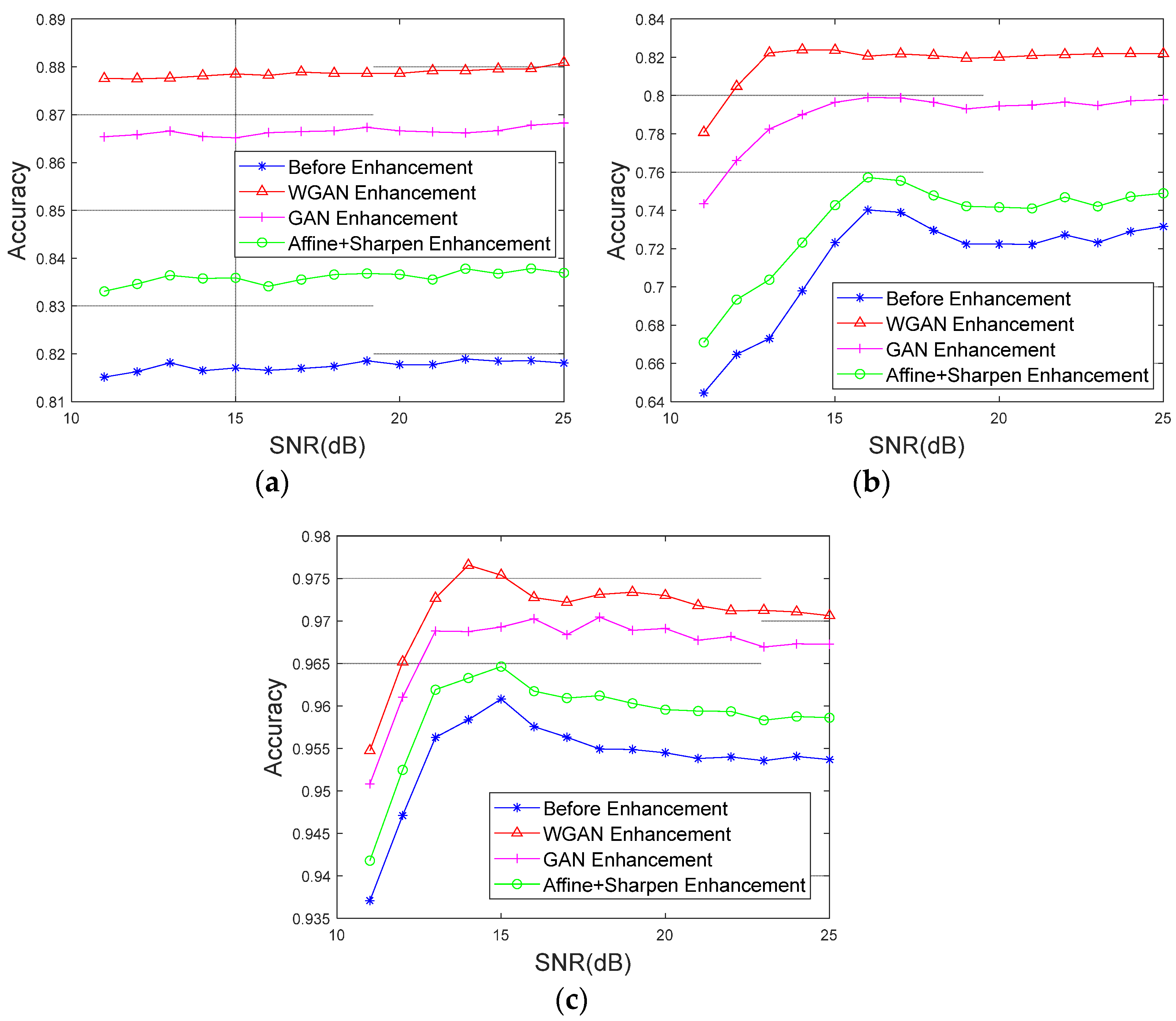
The contrast experiments were conducted under different SNR values, from 11 dB to 25 dB. The GMT-WGAN method was compared with other data enhancement methods. The test accuracies of the three databases of ground moving targets before and after data enhancement by the three methods are shown in Figure 18, where it is observed that for the simulation database based on the modified Boulic model, the test accuracy before enhancement was between 0.81 and 0.82, and the test accuracy after the WGAN data enhancement was between 0.87 and 0.88, indicating an improvement of approximately 0.06; meanwhile, the GAN and affine+sharpening method achieved improvements of only 0.05 and 0.02. In addition, for the semi-measured database obtained from the MOCAP and EM data, when the SNR was between 11 dB and 15 dB, the test accuracy before and after data enhancement showed an upward trend, and the test accuracy was relatively stable when the SNR was between 15 dB and 25 dB. After the WGAN data enhancement, the test accuracy was improved by approximately 0.09, while the improvements achieved by the GAN and affine+sharpening method were approximately 0.065 and 0.02. For the measured data, the test accuracy increased with the SNR value when the SNR value was in the range of 11–15 dB but showed a downward trend when the SNR was between 15 dB and 25 dB. The WGAN method improved the test accuracy by approximately 0.015, while the improvements achieved by the GAN and affine+sharpening method were approximately 0.015 and 0.005.
By comparing the test accuracies of the three databases before and after data enhancement, it can be concluded that the proposed data enhancement method can improve the effectiveness and robustness of the classification network and performs better than the ordinary GAN method and the traditional data enhancement method.

5. Conclusions

In this paper, a classification method of ground moving targets under small dataset conditions based on WGAN and DCNN was proposed. The proposed method uses the WGAN to learn the image data distribution through the confrontation of the generator and discriminator, and augmented samples with statistical characteristics similar to those of the real samples were obtained when the model converges. The original and generated samples were simultaneously fed to the DCNN to train and study different characteristics of various types of ground moving targets. After training, the real samples were fed to the trained DCNN model to test its performance. In this study, seven image quality evaluation metrics were used to measure the similarity in statistical characteristics between the generated and real samples to validate the reliability of generated samples. The effectiveness of the proposed method was verified using the simulation, semi-measured, and measured databases. Finally, the effect of SNR on the classification performance was analyzed, and the superiority and robustness of the proposed method were verified.

Author Contributions

X.Y. and X.S. conceived and designed the experiment and analyzed the data, X.Y. and Y.L. performed the experiments, X.Y. and X.S. wrote the paper, F.Z. and L.W. advised, H.W. and S.R. revised the grammar and technical errors of the paper and gave advice. All authors have read and agreed to the published version of the manuscript.

Funding

This paper was funded in part by the National Natural Science Foundation of China, grant numbers 61801347, 61801344, 62001350, and 61631019; in part by the China Postdoctoral Science Foundation, grant numbers 2017M613076, 2016M602775 and 2020M673346; in part by the Fundamental Research Funds for the Central Universities, grant numbers XJS200212, XJS200210, XJS200204; and by the Natural Science Basic Research Plan in Shaanxi Province of China, grant number 2018JM6051.

Institutional Review Board Statement

Not applicable.

Informed Consent Statement

Informed consent was obtained from all subjects involved in the study.

Data Availability Statement

Not applicable.

Acknowledgments

The authors would like to thank the Associate Editor who handled this paper and the anonymous reviewers for providing valuable comments and suggestions that greatly helped in improving the technical quality and presentation of this paper.

Conflicts of Interest

The authors declare no conflict of interest.

References

  1. Lee, C.; Yoon, C.; Kong, H.; Kim, H.C.; Kim, Y. Heart rate tracking using a doppler radar with the reassigned joint time-frequency transform. IEEE Antennas Wirel. Propag. Lett. 2011, 10, 1096–1099. [Google Scholar]
  2. Kim, Y. Detection of eye blinking using doppler sensor with principal component analysis. IEEE Antennas Wirel. Propag. Lett. 2015, 14, 123–126. [Google Scholar] [CrossRef]
  3. Fioranelli, F.; Ritchie, M.; Griffiths, H. Centroid features for classification of armed/unarmed multiple personnel using multistatic human micro-doppler. IET Radar Sonar Navig. 2016, 10, 1702–1710. [Google Scholar] [CrossRef] [Green Version]
  4. Gurbuz, S.Z.; Clemente, C.; Balleri, A.; Soraghan, J.J. Micro-doppler-based in-home aided and unaided walking recognition with multiple radar and sonar systems. IET Radar Sonar Navig. 2017, 11, 107–115. [Google Scholar] [CrossRef] [Green Version]
  5. Zheng, J.; Chen, R.; Yang, T.; Liu, X.; Liu, H.; Su, T.; Wan, L. An efficient strategy for accurate detection and localization of UAV swarms. IEEE Internet Things J. 2021, 8, 15372–15381. [Google Scholar] [CrossRef]
  6. Zheng, J.; Yang, T.; Liu, H.; Su, T.; Wan, L. Accurate detection and localization of unmanned aerial vehicle swarms-enabled mobile edge computing system. IEEE Trans. Ind. Informat. 2021, 17, 5059–5067. [Google Scholar] [CrossRef]
  7. Zheng, J.; Yang, T.; Liu, H.; Su, T. Efficient data transmission strategy for IIoTs with arbitrary geometrical array. IEEE Trans. Ind. Informat. 2021, 17, 3460–3468. [Google Scholar] [CrossRef]
  8. Chen, V.C.; Li, F.; Ho, S.S.; Wechsler, H. Micro-doppler effect in radar: Phenomenon, model, and simulation study. IEEE Trans. Aerosp. Electron. Syst. 2006, 42, 2–21. [Google Scholar] [CrossRef]
  9. Chen, V.C. The Micro-Doppler Effect in Radar; Artech House: London, UK, 2011. [Google Scholar]
  10. Padar, M.O.; Ertan, A.E.; ĝatay Candan, Ç. Classification of human motion using radar micro-doppler signatures with hidden markov models. In Proceedings of the 2016 IEEE Radar Conference (RadarConf), Philadelphia, PA, USA, 2–6 May 2016; pp. 1–6. [Google Scholar]
  11. Burkan Tekeli, S.Z.G.; Yuksel, M. Information-theoretic feature selection for human micro-doppler signature classification. IEEE Trans. Geosci. Remote Sens. 2016, 54, 2749–2762. [Google Scholar] [CrossRef]
  12. Boulic, R.; Thalmann, N.M.; Thalmann, D. A global human walking model with real-time kinematic personification. Vis. Comput. 1990, 6, 344–358. [Google Scholar] [CrossRef]
  13. Ram, S.; Ling, H. Simulation of human micro-Dopplers using computer animation data. In Proceedings of the 2008 IEEE Radar Conference, Rome, Italy, 26–30 May 2008; pp. 1–6. [Google Scholar]
  14. Barrs Erol, C.K.; Giirbiiz, S.Z. A kinect-based human micro-doppler simulator. IEEE Aerosp. Electron. Syst. Mag. 2015, 30, 6–17. [Google Scholar] [CrossRef]
  15. Yao, X.; Shi, X.; Zhou, F. Human activities classification based on complex-value convolutional neural network. IEEE Sens. J. 2020, 20, 7169–7180. [Google Scholar] [CrossRef]
  16. Björklund, S.; Petersson, H.; Nezirovic, A.; Guldogan, M.B.; Gustafsson, F. Millimeter-wave radar micro-Doppler signatures of human motion. In Proceedings of the 12th International Radar Symposium (IRS), Leipzig, Germany, 7–9 September 2011; pp. 167–174. [Google Scholar]
  17. Mehul, A.; Kernec, J.L.; Gurbuz, S.Z.; Fioranelli, F. Sequential human gait classification with distributed radar sensor fusion. IEEE Sens. J. 2021, 21, 7590–7603. [Google Scholar]
  18. Garreau, G.; Nicolaou, N.; Andreou, C.; Urbal, C.D.; Stuarts, G.; Georgiou, J. Computationally efficient classification of human transport mode using micro-doppler signatures. In Proceedings of the 45th Annual Conference on Information Sciences and Systems, Baltimore, MD, USA, 23–25 March 2011; pp. 1–4. [Google Scholar]
  19. Lshibashi, N.; Fujii, F. Hidden Markov model-based human action and load classification with three-dimensional accelerometer measurements. IEEE Sens. J. 2021, 21, 6610–6622. [Google Scholar] [CrossRef]
  20. Fairchild, D.P.; Narayanan, R.M. Classification of human motions using empirical mode decomposition of human micro-Doppler signatures. IET Radar Sonar Navig. 2014, 8, 425–434. [Google Scholar] [CrossRef]
  21. Amin, M.G.; Ahmad, F.; Zhang, Y.D.; Boashash, B. Human gait recognition with cane assistive device using quadratic time-frequency distributions. IET Radar Sonar Navig. 2015, 9, 1224–1230. [Google Scholar] [CrossRef] [Green Version]
  22. McDonald, M.K. Discrimination of human targets for radar surveillance via micro-Doppler characteristics. IET Radar Sonar Navig. 2015, 9, 1171–1180. [Google Scholar] [CrossRef]
  23. Kim, Y.; Ha, S.; Kwon, J. Human detection using doppler radar based on physical characteristics of targets. IEEE Geosci. Remote Sens. Lett. 2015, 12, 289–293. [Google Scholar]
  24. Bryan, J.D.; Kwon, J.; Lee, N.; Kim, Y. Application of ultra-wide band radar for classification of human activities. IET Radar Sonar Navig. 2012, 6, 172–179. [Google Scholar] [CrossRef]
  25. Kim, Y.; Ling, H. Human activity classification based on micro-Doppler signatures using a support vector machine. IEEE Trans. Geosci. Remote Sens. 2009, 47, 1328–1337. [Google Scholar]
  26. Nanzer, J.A.; Rogers, R.L. Bayesian classification of humans and vehicles using micro-Doppler signals from a scanning-beam radar. IEEE Microw. Wirel. Compon. Lett. 2009, 19, 338–340. [Google Scholar] [CrossRef]
  27. Du, L.; Ma, Y.; Wang, B.; Liu, H. Noise-robust classification of ground moving targets based on time-frequency feature from micro-doppler signature. IEEE Sens. J. 2014, 14, 2672–2682. [Google Scholar] [CrossRef]
  28. Shi, X.; Zhou, F.; Liu, L.; Zhao, B.; Zhang, Z. Textural feature extraction based on time–frequency spectrograms of humans and vehicles. IET Radar Sonar Navig. 2015, 9, 1251–1259. [Google Scholar] [CrossRef]
  29. Kim, Y.; Park, J.; Moon, T. Classification of micro-doppler signatures of human aquatic activity through simulation and measurement using transferred learning. In Radar Sensor Technology; International Society for Optics and Photonics: Bellingham, WA, USA, 2017; Volume 10188, p. 101880V. [Google Scholar]
  30. Kim, Y.; Toomajian, B. Hand gesture recognition using micro-Doppler signatures with convolutional neural network. IEEE Access 2016, 4, 7125–7130. [Google Scholar] [CrossRef]
  31. Bjerrum, E.J. SMILES enumeration as data augmentation for neural network modeling of molecules. arXiv 2017, arXiv:1703.07076. [Google Scholar]
  32. Song, Q.; Xiong, R.; Liu, D.; Wu, F.; Gao, W. Fast image super-resolution via local adaptive gradient field sharpening transform. IEEE Trans. Image Processing 2018, 27, 1966–1980. [Google Scholar] [CrossRef]
  33. Goodfellow, I.J.; Pouget-Abadie, J.; Mirza, M.; Xu, B.; Warde-Farley, D.; Ozair, S.; Courville, A.; Bengio, Y. Generative adversarial nets. In Proceedings of the International Conference on Neural Information Processing Systems, Montreal, QC, Canada, 8–13 December 2014; pp. 2672–2680. [Google Scholar]
  34. Seyfioğlu, M.S.; Özbayoğlu, A.M.; Gürbüz, S.Z. Deep convolutional autoencoder for radar-based classification of similar aided and unaided human activities. IEEE Trans. Aerosp. Electron. Syst. 2018, 54, 1709–1723. [Google Scholar] [CrossRef]
  35. Alnujaim, I.; Oh, D.; Kim, Y. Generative adversarial networks for classification of micro-Doppler signatures of human activity. IEEE Geosci. Remote Sens. Lett. 2019, 17, 396–400. [Google Scholar] [CrossRef]
  36. Erol, B.; Burbuz, S.Z.; Amin, M.G. Motion classification using kinematically sifted ACGAN-synthesized radar micro-Doppler signatures. IEEE Trans. Aerosp. Electron. Syst. 2020, 56, 3197–3213. [Google Scholar] [CrossRef] [Green Version]
  37. Alnujaim, I.; Ram, S.S.; Oh, D.; Kim, Y. Synthesis of micro-Doppler signatures of human activities from different aspect angles using generative adversarial networks. IEEE Access 2021, 9, 46422–46429. [Google Scholar] [CrossRef]
  38. Arjovsky, M.; Bottou, L. Towards principled methods for training generative sdversarial networks. arXiv 2017, arXiv:1701.04862. [Google Scholar]
  39. Magister, L.C.; Arandjelović, O. Generative Image Inpainting for Retinal Images using Generative Adversarial Networks. In Proceedings of the Annual International Conference of the IEEE Engineering in Medicine & Biology Society, Guadalajara, Mexico, 1–5 November 2021. [Google Scholar]
  40. Fu, Y.; Zheng, C.; Yuan, L.; Chen, H.; Nie, J. Small Object Detection in Complex Large Scale Spatial Image by Concatenating SRGAN and Multi-Task WGAN. In Proceedings of the International Conference on Big Data Computing and Communication, Deqing, China, 13–15 August 2021. [Google Scholar]
  41. Shi, X.; Yao, X.; Bai, X.; Zhou, F.; Li, Y.; Liu, L. Radar echoes simulation of human movements based on MOCAP data and EM calculation. IEEE Geosci. Remote Sens. Lett. 2019, 16, 859–863. [Google Scholar] [CrossRef]
Figure 1. The GAN architecture.
Remotesensing 14 00123 g001
Figure 2. The DCGAN architecture. (a) Generator; (b) discriminator.
Remotesensing 14 00123 g002
Figure 3. The flowchart of the proposed GMT-WGAN classification method.
Remotesensing 14 00123 g003
Figure 4. The WGAN discriminator architecture.
Remotesensing 14 00123 g004
Figure 5. The DCNN architecture.
Remotesensing 14 00123 g005
Figure 6. The time–frequency spectrograms of the simulation database based on the modified Boulic model. (a) Unarmed pedestrian; (b) armed pedestrian.
Remotesensing 14 00123 g006
Figure 7. The time–frequency spectrograms of the semi-measured database. (a) Walking; (b) running; (c) jumping.
Remotesensing 14 00123 g007
Figure 8. The time–frequency spectrograms of the measured data. (a) Pedestrian; (b) vehicle.
Remotesensing 14 00123 g008
Figure 9. Generated samples of the pedestrian database obtained using the modified Boulic model. (a) Armed pedestrian; (b) unarmed pedestrian.
Remotesensing 14 00123 g009
Figure 10. Generated samples of the semi-measured pedestrian postures database obtained from the MOCAP and EM data. (a) Walking; (b) jumping; (c) running.
Remotesensing 14 00123 g010
Figure 11. Generated samples of the measured pedestrian and vehicle target data. (a) Pedestrian; (b) vehicle.
Remotesensing 14 00123 g011
Figure 12. Bar graphs of the seven evaluation metrics of the generated samples from the database obtained using the modified Boulic model: (a) Armed pedestrian; (b) unarmed pedestrian.
Remotesensing 14 00123 g012
Figure 13. Bar graphs of the seven evaluation metrics of the generated samples from the database obtained from the MOCAP and EM data: (a) Walking; (b) jumping; (c) running.
Remotesensing 14 00123 g013
Figure 14. Bar graphs of the seven evaluation metrics of the generated samples from the database obtained from the measured data: (a) Pedestrian; (b) vehicle.
Remotesensing 14 00123 g014
Figure 15. Generated samples obtained by the affine+sharpening method using the modified Boulic model. (a) The original image; (b) affine (reflex); (c) sharpening.
Remotesensing 14 00123 g015
Figure 16. Generated samples obtained by the affine+sharpening method from the MOCAP and EM data. (a) The original image; (b) affine (reflex); (c) sharpening.
Remotesensing 14 00123 g016
Figure 17. Generated samples obtained by the affine+sharpening method from the measured data. (a) The original image; (b) affine (reflex); (c) sharpening.
Remotesensing 14 00123 g017
Figure 18. Comparison of the test accuracy before and after data enhancement under different SNR values. (a) Simulation data; (b) semi-measured data; (c) measured data.
Remotesensing 14 00123 g018
Table 1. Armed and unarmed pedestrian walking database construction parameters.
ParameterValueParameterValue
Radar Parameters
Carrier frequency35 GHzBandwidth4500 MHz
Location of transmitting antenna(67, 40, 2)Location of receiving antenna(67, −40, 2)
PRF4 kHz
Target Parameters
Relative velocity0.1–3 m/sHeight1.6–1.8
Initial location(0, 0, 0)Number of cycles1
Database Parameters
Image size512 × 512AttributeGray
Number of armed people200Number of unarmed people200
Table 2. Parameters of measured data.
VehiclePedestrian
WaveformBandwidth (MHz)/
Period (ms)
Number of EchoesWaveformBandwidth (MHz)/
Period (ms)
Number of Echoes
Sawtooth5/124Sawtooth10/14
Sawtooth10/148Sawtooth15/43
Sawtooth100/112Sawtooth100/412
Triangular5/224Triangular10/212
Triangular10/212Triangular15/810
Total 120Total 41
Table 3. The WGAN model parameters.
Image size256 × 256AttributeGray
Epoch5000Learning rate0.005
Weights clipping range[−0.01, 0.01]OptimizerRMSProp
Table 4. Values of the seven evaluation metrics of the generated samples from the database based on the modified Boulic model.
MeanVarianceEntropyDynamic ZoneLIFAGGLD
PostureArmed
Real samples0.02450.070910.47950.19990.01870.00120.0029
Generated samples (WGAN)0.03310.08938.56990.20730.02390.00260.0089
Generated samples (GAN)0.3530.09138.48360.20240.03180.00170.0086
PostureUnarmed
Real samples0.02590.070010.56150.20910.01830.00130.0029
Generated samples (WGAN)0.03240.08478.52040.20900.02590.00240.0066
Generated samples (GAN)0.03550.08458.44260.21300.03160.00140.0070
Table 5. Values of the seven evaluation metrics of the generated samples from the database obtained from the MOCAP and EM data.
MeanVarianceEntropyDynamic ZoneLIFAGGLD
PostureWalking
Real samples0.08580.190110.97360.24490.05970.00290.0120
Generated samples (WGAN)0.08560.18779.54390.25220.06110.00470.0208
Generated samples (GAN)0.08470.18049.97230.24560.05480.00450.0187
PostureJumping
Real samples0.05210.161410.48910.15250.02860.00180.0075
Generated samples (WGAN)0.04330.13067.26530.12670.02560.00260.0113
Generated samples (GAN)0.04320.14547.26480.13580.02700.00240.0112
PostureRunning
Real samples0.06160.169410.54280.15520.04440.00220.0090
Generated samples (WGAN)0.02140.05993.27100.05320.01560.00130.0055
Generated samples (GAN)0.03040.05483.27050.05190.01670.00160.0049
Table 6. Values of the seven evaluation metrics of the generated samples from the measured data.
MeanVarianceEntropyDynamic ZoneLIFAGGLD
Target typePedestrian
Real samples0.08010.094911.25330.35860.03700.00480.0130
Generated samples (WGAN)0.08220.098110.57270.36520.04270.00500.0133
Generated samples (GAN)0.08470.127411.24650.35740.03210.00350.0104
Target typeVehicle
Real samples0.04420.087610.88080.21330.02040.00290.0091
Generated samples (WGAN)0.04500.084510.26340.25640.02300.00280.0114
Generated samples (GAN)0.04520.099110.89260.25320.02570.00200.0087
Table 7. Parameters of the classification network and samples.
Classification Network Parameters
Input size[256,256,1]Epoch500
Learning rate0.001OptimizerAdam
Sample parameters
Simulation data
Training set (Before expansion)40 (10%)Training set (After expansion)2040 (10% + Expansion)
Test set360 (90%)Number of categories2
Semi-measured data
Training set (Before expansion)12 (10%)Training set (After expansion)612 (10% + Expansion)
Test set120 (90%)Number of categories3
Measured data
Training set (Before expansion)34 (10%)Training set (After expansion)1734 (10% + Expansion)
Test set317 (90%)Number of categories2
Publisher’s Note: MDPI stays neutral with regard to jurisdictional claims in published maps and institutional affiliations.