Article

Direct Georeferencing UAV-SfM in High-Relief Topography: Accuracy Assessment and Alternative Ground Control Strategies along Steep Inaccessible Rock Slopes

by
Paul Ryan Nesbit
1,*,
Stephen M. Hubbard
1 and
Chris H. Hugenholtz
2
1
Department of Geoscience, University of Calgary, 2500 University Drive NW, Calgary, AB T2N 1N4, Canada
2
Department of Geography, University of Calgary, 2500 University Drive NW, Calgary, AB T2N 1N4, Canada
*
Author to whom correspondence should be addressed.
Remote Sens. 2022, 14(3), 490; https://doi.org/10.3390/rs14030490
Submission received: 9 December 2021 / Revised: 31 December 2021 / Accepted: 17 January 2022 / Published: 20 January 2022

Abstract

:
Steep rock slopes present key opportunities and challenges within Earth science applications. Due to partial or complete inaccessibility, high-precision surveys of these high-relief landscapes remain a challenge. Direct georeferencing (DG) of unoccupied aerial vehicles (UAVs) with advanced onboard GNSS receivers presents opportunities to generate high-resolution 3D datasets without ground-based access to the study area. However, recent research has revealed large vertical errors using DG that may prove problematic in near-vertical terrain. To address these concerns, we examined more than 75 photogrammetric UAV-datasets with various imaging angles (nadir, oblique, and combinations) and ground control scenarios, including DG, along a steep slope exposure. Results demonstrate that mean errors in DG scenarios are up to 0.12 m higher than datasets using integrated georeferencing with well-distributed GCPs. Inclusion of GCPs greatly reduced mean error values but had limited influence on precision (<0.01 m) for any given imaging strategy. Use of multiple image angles resulted in the highest precisions, regardless of georeferencing strategy. These findings have implications for applications requiring the highest precision and accuracy (e.g., geotechnical engineering, hazard mitigation and mapping, and geomorphic change detection), which should consider using ground control whenever possible. However, for applications less concerned with absolute accuracy, our results show that DG datasets provide strong internal consistency and relative accuracy that may be suitable for high precision measurements within a model, without use of ground control.

1. Introduction

Steep slopes are common natural landscape features that provide recreational and educational opportunities, but also pose a number of geotechnical challenges. Sub-vertical slopes can afford some of the best outcrop exposures and offer a viewing window into laterally extensive geologic features that are commonly not exposed at the surface. However, slopes are also dynamic and particularly susceptible to contemporary erosional processes, often posing safety hazards to people and infrastructure. Due to partial or complete inaccessibility, quantitative documentation of these high-relief landscapes is challenging for established surveying methods that commonly require ground-based measurements.
Remote sensing techniques, such as light detection and ranging (LiDAR) and photogrammetry, are commonly used to record detailed 3-dimensional (3D) information of inaccessible slopes in academic, commercial, and public safety applications. Ground-based LiDAR, also referred to as terrestrial laser scanning (TLS), is considered the standard for recording reliable 3D information about a scene, while preserving geometric properties (i.e., scale, orientation, dimensions) [1,2]. TLS is particularly well-suited to steeply sloping planes and façades when compared to conventional airborne surveys with nadir look angles [3,4] and has been used in geotechnical engineering [5,6,7] and geologic [8,9,10] applications. However, TLS can be hindered by practical issues, such as limited mobility, high costs, and susceptibility to occlusions created by restricted line-of-sight [10,11].
Photogrammetry is a popular low-cost alternative for recording datasets along steep slopes, particularly with recent advances in automated image matching algorithms, such as structure-from-motion and multi-view stereo (SfM-MVS) [12,13]. Images collected from unoccupied aerial vehicles (UAV) are now commonly processed using SfM-MVS workflows (UAV-SfM) to create digital datasets of inaccessible and/or extensive areas with detailed resolution and ground sampling distance (GSD) in geomorphic [14,15,16,17,18,19,20], geologic [21,22,23,24,25,26,27,28,29,30], and geotechnical [31,32,33,34] studies.
However, photogrammetry depends on known ground control points (GCPs) within a given study area for reliable absolute accuracy (i.e., location and orientation), relative accuracy (i.e., reconstruction of internal scene morphology), and camera calibration (i.e., interior orientation parameters) accuracy [35,36]. Following established recommendations in photogrammetry, GCPs should be well-distributed and non-colinear throughout a scene to constrain the full survey area, including the periphery [37]. Several investigations have documented UAV-SfM accuracy based on GCP distribution and precision [38,39,40,41,42,43,44], but rarely consider the practical challenges and potential hazards in high-relief terrain. Measuring GCPs in scenes with steep slopes may require additional equipment, such as total station, to record points along a façade [2,11,32], or use of relative reference systems [45,46].
Direct georeferencing (DG) using on-board GNSS has potential to increase survey efficiency and has demonstrated success using ground-based sensors [5,47,48], but is often unreliable due to low-precision (~5–10 m) consumer positioning systems [49,50,51]. However, precise positioning using multi-carrier phase GNSS capabilities is becoming increasingly available for UAVs, colloquially known as real-time kinematic, or RTK-UAVs. Evaluation of RTK-UAVs commonly indicate that datasets using GCPs are more accurate than DG datasets, specifically in the vertical (z) vector [51,52,53,54,55,56,57,58,59,60,61,62,63,64], attributed to suboptimal estimation of camera interior orientation parameters (IOPs), notably focal length, during self-calibration [59,65]. Although strategies to reduce vertical bias have been suggested using a single GCP [54,59,64,66,67], oblique images [55,68,69], or alternative IOP calibration [38,70,71], few studies (e.g., [53,56]) have considered how vertical errors manifest in datasets with vertically oriented objects and extensive vertical landscape features.
To evaluate the accuracy and precision of RTK-UAV photogrammetric datasets along laterally extensive sub-vertical rock slopes, we compare absolute and relative accuracy of more than 75 scenarios. Variables include orthogonal and nadir imaging angles combined with various GCP strategies, including direct georeferencing using RTK-UAV image geolocation and use of image geolocation combined with GCPs (integrated georeferencing). UAV datasets are compared against a TLS reference dataset to document disparities in absolute positioning and relative internal precision of 3D photogrammetric datasets.

2. Materials and Methods

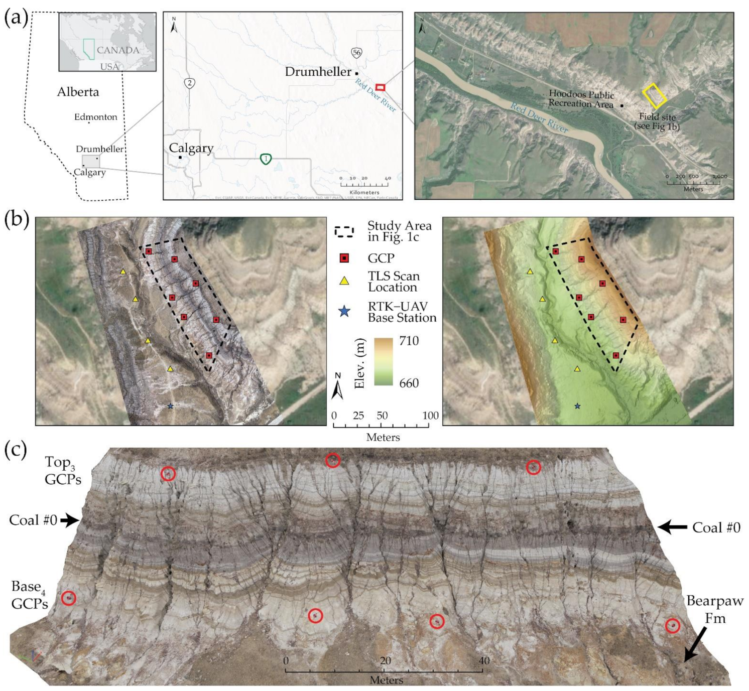
2.1. Study Area and Geologic Setting

To test the performance of DG UAV-SfM across near-vertical planes, we selected a section of outcrop exposure along a steep slope (approximately 70° on average) near the Hoodoos Public Recreation Area, 12 km southeast of Drumheller, Alberta (Figure 1). The outcrop exposes extensive channel system deposits of the Late Cretaceous Horseshoe Canyon Formation (Campanian-Maastichtian) that is well-exposed for tens of kilometers throughout the Red Deer River valley [72,73,74,75,76,77]. Within the field area specifically, deposits have been identified as meander-belt strata with packages of distinct inclined heterolithic stratification signifying lateral point-bar migration [72,74,78] along with fine-grained deposits indicating transition to counter-point-bar deposits and associated abandoned channel fill [79]. Locally, the underlying marine dominated Bearpaw Formation can be found at the erosional base of the Horseshoe Canyon (Figure 1c) along with regionally identifiable features, such as Coal #0 [76,80,81], which is ~0.8 m thick locally and can be followed continuously for tens of kilometers throughout the Red Deer River valley [79].

2.2. UAV Data Acquisition

UAV images were collected using a DJI Phantom 4 RTK quadcopter (P4RTK) equipped standard with 1″ sensor, 20 megapixel, and 8.8 mm focal length, equating to approximately 0.014 m/pix at 50 m altitude above ground level. The camera is integrated into the UAV system on a 3-axis gimbal that can be tilted from −90° (nadir) to 0° (horizontal) along the x-axis, enabling complete coverage within complex, sloping topography. The P4RTK system includes high-precision GNSS receivers compatible with multiple constellations and frequencies, including: GPS (L1/L2), GLONASS (L1/L2), Galileo (E1/E5a), and Beidou (B1/B2) with horizontal and vertical precisions of 0.01 and 0.015 m, respectively [82].
There are various RTK configurations for the P4RTK, we use the D-RTK 2 Mobile Station configuration in classic RTK-mode to facilitate: (1) automatic geotagging of images with high-precision locations that do not require post processing, and (2) manual flight mode, which is not compatible with post processing kinematic workflows. The D-RTK 2 is capable of establishing its position prior to flight, but a workflow for highest precision using post processing is not well-documented. Therefore, the D-RTK 2 base station was setup over a known ground control point surveyed with a Trimble R8 RTK-GNSS and post-processed using Natural Resources Canada—Precise Point Positioning service to enhance precision through precise GNSS orbit and clock information [83]. Setup of RTK mode, positioning, and manual flights were conducted using the DJI GS RTK application integrated with the P4RTK flight controller.
Experimental UAV-SfM and reference TLS datasets were collected nearly simultaneously during a cloudy day with consistently dissipated lighting conditions throughout the survey. Prior to UAV flights, 7 GCP targets were distributed at the base and along an accessible ridge at the top of the slope (Figure 1b,c). GCPs were 0.6 m × 0.6 m corrugated plastic with quadrants painted alternating red and black forming a distinct central point. Center points of non-signalized GCPs were measured using a Trimble R8 RTK-GNSS system with base receiver placed on the established known control point and GCPs measured with the rover in RTK-mode. UAV images were collected during 3 different flights, each with a single image angle and varying distance from outcrop: nadir (−90°, ~60 m average), oblique (−60°, 50 m), and obliqueclose (−45°, 32 m; Table 1).

2.3. UAV-SfM Processing

All UAV-SfM datasets were processed using Pix4Dmapper (v4.5.6) on a high-performance computer. An initial ‘master’ project was created with image sets from each flight (nadir, oblique, and obliqueclose) and all GCPs with precision information from respective GNSS instrumentation (Table 1). Each GCP was manually verified in six images for each imaging angle (18 images total) within Pix4Dmapper GCP Manager. To ensure consistency of GCP marks among processing scenarios, each dataset was then derived from this master project, creating 77 unique datasets from varying combinations of image angle (Table 1) and georeferencing strategy. Scenarios processed without GCPs are equivalent to DG using only RTK-UAV location information in SfM-MVS processing. Datasets that incorporate one or more GCP are equivalent to integrated georeferencing as they include both GCP and RTK-UAV image location information in processing, sometimes referred to as assisted georeferencing. GCP configurations were selected to represent common real-world scenarios in which accessibility around a slope or cliff varies; for example, accessibility limited to the base of a slope (Base4), top of a slope (Top3), and a single GCP based on recommendations from previous studies [53,54,59,64,66,67].
To facilitate matching among images with nadir and oblique perspectives and high-precision image location, a number of customized settings were adapted in SfM-MVS processing (Table 2). Default calibration settings were modified to use “Accurate Geolocation and Orientation” and IOP Optimization was changed from “All” to “All Prior,” as recommended by Pix4D for image sets with high-precision location information [71,84]. According to the software developer, this forces IOP values that are iteratively re-calculated and optimized during bundle adjustment to be similar to initial values. In some instances, this setting has been tested and found to degrade accuracy of results [71] but similar pre-processing in our datasets did not result in any notable differences.

2.4. Reference Datasets

Reference datasets were collected nearly simultaneously with GCP and UAV surveys using a FARO Focus3D S120 TLS. The FARO is a phase-based laser scanner (905-nm wavelength) that can record up to 976,000 points per second at precisions of 0.002 m at 25 m target distance and angular resolution of 0.011° [85]. To mitigate occlusions and data shadows in TLS point clouds, a total of four scans were collected with substantial overlap of the 125 m × 55 m slope. Scans were imported, processed, and georeferenced within FARO Scene v7.0.2.5 software following similar process documented in [34]. Initial scan locations were surveyed in the field using the Trimble R8 RTK system described previously and combined with orientation measurements from internal TLS sensors. Relative registration and merging were performed using cloud-to-cloud registration functions within FARO Scene software. The merged point cloud was then aligned to absolute geospatial coordinates through indirect georeferencing using the seven GCPs that were also used for referencing UAV-SfM datasets (described previously). Center points on GCPs were identified in the point cloud (Figure 2) and used to perform a global shift, which involves translation and rotation without modification to scale. To reduce noise in SfM and TLS datasets caused by sparse vegetation [86,87,88], the reference TLS point cloud was filtered to remove collocated points (within 0.004 m) and obvious patches of vegetation using the CANUPO plugin [89] in open-source CloudCompare software [90]. The final reference point cloud contained 10.4 million points, a registration error of 0.014 m, and an average point density of 1950 pts/m3.

2.5. Assessment

To compare the experimental UAV-SfM and reference TLS point clouds, we used the Multiscale Model to Model Cloud Comparison (M3C2) plugin for CloudCompare [91]. M3C2 reports differences between two point clouds based on local surface roughness and surface normal orientation within a user defined radius. Local differences are calculated by estimating an average plane for each point cloud within the given radius and subsequently calculating the distance between each plane, see [91] for detailed description. M3C2 is ideal for identifying 3D variance throughout an entire point cloud surface and is particularly effective at identifying local differences in complex topography. In our comparisons, we followed a similar workflow to previous studies (e.g., [91,92]; however, to ensure proper normal orientation, surface normals of the TLS reference point cloud were calculated prior to M3C2 calculation. Normals were calculated using the Compute Normals function in CloudCompare, with parameters set to Quadric surface approximation, Octree of 0.1 m radius (to align with M3C2 diameter), and orientation using Minimum Spanning Tree knn = 16. Calculated normals were then used in all M3C2 calculations for Cloud 1 (TLS) normal. Additional parameters used in M3C2 calculation include the TLS registration error (0.014 m), defined projection diameter (d) of 0.1 m, and a maximum depth of 3.0 m. Output datasets from M3C2 processing provide localized differences between the TLS reference point cloud and each UAV-SfM point cloud in the direction of local surface normals.

3. Results

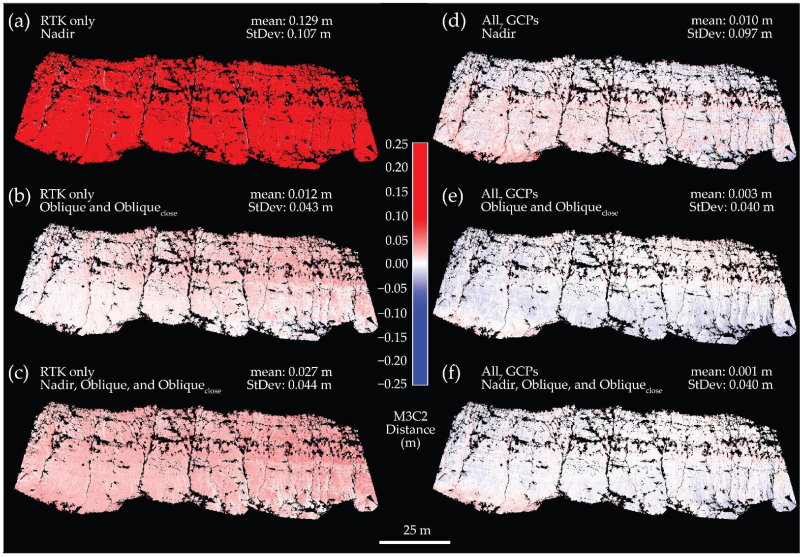
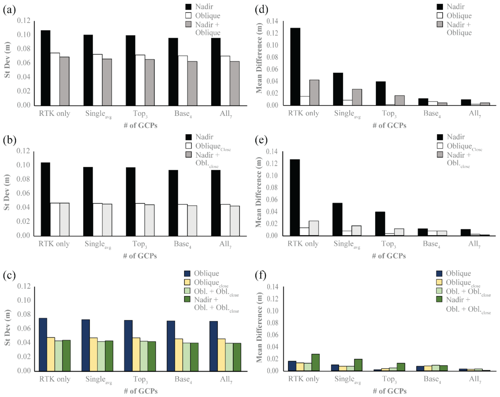
3.1. Direct and Integrated Georeferencing

Dense point clouds processed using DG strategy resulted in the highest standard deviations and mean values when compared to scenarios processed with one or more GCP for each imaging angle (Figure 3 and Figure 4). The addition of GCPs had minimal impact on standard deviations for each imaging angle (Figure 4a). For example, nadir-only datasets demonstrated the largest change in standard deviation from DG (0.107 m) to use of All7 GCPS (0.097 m; Figure 3a,d); similarly, combination scenarios, such as oblique + obliqueclose ranged from 0.043 m to 0.040 m for the same georeferencing strategies (Figure 3b,e). The number of GCPs had a greater influence on mean difference values for each imaging angle (Figure 4b), with considerable improvements in nadir datasets (DG = 0.129 m and All7 GCPs = 0.010 m) and smaller refinements for combination datasets (Figure 3). Generally, inclusion of more GCPs resulted in lower error values for a given imaging scenario, with the exception of the oblique-only scenarios that had similar mean values for All7 and Top3 GCP scenarios.

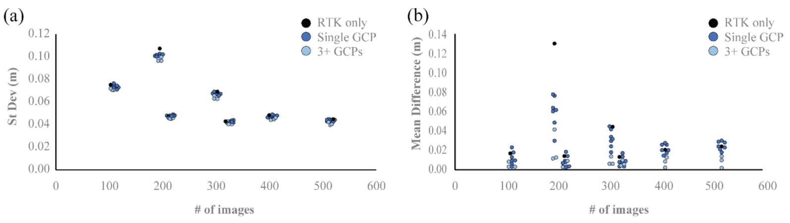
3.2. Imaging Variables

Nadir-only datasets produced higher standard deviations than all datasets in this investigation, regardless of georeferencing strategy, and had higher mean error values than all other imaging angles unless at least four GCPs were used. Combining nadir- and oblique- images resulted in lower standard deviation than single-angle datasets for all georeferencing strategies (Figure 5a–c). Mean error values were higher in datasets containing nadir images (e.g., nadir-only and combined nadir/oblique) compared to oblique-only datasets, particularly when processed with fewer than four GCPs (Figure 5d–f).
UAV-SfM models produced from larger image sets typically resulted in lower standard deviations for all georeferencing scenarios (Figure 6a). Number of images used in UAV-SfM processing had little impact on mean difference errors (Figure 6b). Image sets with higher proportions of nadir images resulted in higher standard deviations and mean difference values for all georeferencing strategies, particularly in single GCP and no GCP scenarios (Figure 7).

4. Discussion

Our study confirms that GCPs are generally beneficial for SfM-MVS processing relative to DG strategies, even when implementing an RTK-enabled UAV. This aligns with previous studies comparing DG to various georeferencing strategies and extends understanding from relatively flat, horizontal scenes, to complex landscapes with laterally extensive sub-vertical planes common to geologic, geomorphic, and geotechnical engineering applications.
Statistical analysis of surface errors calculated by M3C2 offers insight into the internal precision of a 3D dataset and absolute accuracy relative to global geographic coordinates. In our analyses, standard deviation indicates how widely dispersed error values are between a given UAV-SfM dataset and the reference TLS dataset. For example, a low standard deviation suggests that difference values are relatively consistent throughout a model, while a high standard deviation indicates a broader range of errors. Two datasets with similar standard deviations have similar internal consistency, but may show differences in absolute accuracy based on mean values. A mean value close to zero suggests the UAV-SfM model is roughly aligned with the TLS reference, while a mean further from zero may be ‘offset’ from the reference surface via error in positional placement, such as global shift, translation, or rotation [93,94]. In our study, use of GCPs improves resulting mean error values by aligning UAV-SfM and TLS datasets, but does not have a notable influence on standard deviation values. Imaging geometry has a more profound impact on standard deviation and internal consistency of 3D datasets, but may also reduce absolute accuracy unless sufficient number of GCPs are included in SfM-MVS processing.

4.1. Absolute Accuracy

Regardless of imaging geometry, the use of GCPs improved mean M3C2 error values (i.e., values closer to 0) relative to DG. Datasets without GCPs consistently resulted in the highest mean error values, while increasing the number of GCPs in a given imaging scenario generally improved mean M3C2 values, with best results generated in scenarios using All7 GCPs (Figure 3 and Figure 4). Including a single GCP had mixed results, lowering mean values in 82% of scenarios and reducing mean errors by >50% in nearly a quarter of scenarios compared to DG. Distribution of GCPs along the Top3 or Base4 of the slope had more consistent results with lower mean values than 40 of 49 single GCP (and all DG) scenarios with 12 of 14 scenarios reducing mean error by >50% compared to DG. Quantitatively, All7 GCPs resulted in mean error values at least four times smaller than RTK-only for all imaging scenarios.
These findings suggest that GCPs measured with survey-grade GNSS are imperative for the highest absolute accuracy and alignment of SfM-MVS models with geospatial coordinates, even when employing an RTK-UAV. This further supports recent studies that document shortcomings of DG using RTK-UAV images compared to datasets incorporating GCPs in relatively flat landscapes [51,52,53,54,55,56,57,58,59,60,61,62,63,64]. Errors in DG are often attributed to a lack of reliable precision (or physical offset) of onboard GNSS measurements and/or incorrect camera calibration during bundle adjustment. To mitigate errors and vertical biases, many studies have suggested inclusion of a single GCP [54,59,64,66,67]. Similar to previous work, our results demonstrate that a single GCP often improves mean error values, by shifting the mean closer to zero; however, results appear inconsistent and generally provide minor improvements. Differences between our results and previous investigations may be due to different weighting of precision parameters for images and/or GCPs within SfM-MVS processing, placement of GCP within the scene, and/or could be partly attributed to the vertical orientation of the study area.
Distribution of multiple GCPs along the top or base of a slope has also been suggested when a slope is partially inaccessible. Regardless of imaging geometry, our results show substantial improvement and consistent reduction of mean error when at least three GCPs are incorporated with RTK-UAV images. These outcomes are based on two different GCP configurations that are roughly linear and at similar elevations, which is generally considered poor GCP distribution when using low-precision GNSS observations typical of consumer UAVs [31]. However, in combination with RTK-UAV images, this solution may present a viable alternative for surveying challenging terrain when distribution of GCPs throughout an entire slope/site is not possible.

4.2. Relative Accuracy

In addition to improving model alignment to absolute geospatial coordinates, inclusion of GCPs also appears to have a minor influence on resulting standard deviation. Although, increasing number of GCPs consistently lowered standard deviation values (improved precision) within datasets of a given imaging angle, differences were only a fraction of GSD (<65% GSD; Figure 4a). These apparent improvements of less than 1 GSD may not be reliably distinguishable from random errors and noise within a dataset [95]. The narrow difference of standard deviation relative to inclusion/exclusion of GCPs in our study suggests that it is possible to generate 3D models with strong internal consistency using RTK-UAV images, regardless of georeferencing strategy. These results appear consistent with previous literature in demonstrating that inclusion of precise image positions mitigates block deformation issues [96]. Our results are also analogous to the simulations performed by James et al. (2017) [94] showing that the internal shape of a reconstructed topographic surface could be accurate, while larger overall errors can propagate due to poor georeferencing to an external coordinate system, i.e., strong relative accuracy and poor absolute accuracy.
Imaging angle had a strong influence on the internal precision of 3D models (Figure 4a and 5a–c). The highest standard deviations occurred in datasets using only nadir images, regardless of georeferencing strategy (min = 0.097 m, max = 0.107 m). This could be partially attributed to the poor perspective of images, highly oblique and non-normal to the dominant topographic exposure of sloping terrain. In photogrammetric surveys, it is not common practice to collect a majority of images at highly oblique angles relative to the plane of interest. However, collection of nadir images along parallel flight lines is the most common practice in UAV-SfM operations, particularly for large areas [97], and may be the default implementation for operators unaware of the challenges presented by high-relief terrain.
Tilting the camera to align the image plane roughly parallel with the average slope is a practical UAV-SfM surveying strategy to acquire more detailed datasets along steep slopes that has been recently applied [20,32,98]. In our study, use of similar imaging strategies (e.g., oblique and obliqueclose) also yielded improvements to dataset precision with standard deviations of 0.073 m and 0.047 m respective averages, compared to nadir datasets (0.101 m). Lowest standard deviations were produced by datasets that combined nadir and oblique imaging geometries, particularly those that included obliqueclose images, with minimum of 0.040 m and maximum of 0.049 m. This is consistent with recent studies that have documented the benefits of adding oblique images to nadir image blocks to obtain wide parallactic angles among images that are beneficial in reducing systematic internal errors [92,94,99]. Compared to the addition of GCPs, our results demonstrate that creating strong image network geometry with RTK-UAV images is more effective for improving the internal precision of UAV-SfM models.

4.3. Additional Factors

The number and ratio of images collected at different angles may contribute to disparities in standard deviation and mean error values. Including more images typically corresponds with higher overlap and greater redundancy within images that can result in higher precision and accuracy [94,96,100,101]. In our study, increasing the number of images does not appear to have a direct relationship with accuracy, but generally produces results with lower standard deviations (Figure 6). However, the ratio of images collected at different angles may have a more distinct impact on accuracy. Previous studies have documented the general benefits of incorporating multiple imaging angles in camera self-calibration while cautioning that unbalanced ratios can shift mean error values away from zero [92,93]. Results in this study seem consistent with previous findings that increasing the proportion of images non-normal to the primary object plane (nadir images in this study) produced mean values further from zero, compared to parallel imaging geometries (Figure 7). This relationship is most prevalent in RTK-only and single GCP scenarios and was partially mitigated by use of three or more GCPs (Figure 7). Though our results highlight potential correlation among variables previously speculated upon, further research is required to thoroughly vet and document these relationships before any reliable recommendation is made regarding DG UAV survey techniques and ideal image network geometry.
Variables that are not further considered here are processing settings and handling of input parameters, such as image location/orientation precision and GCP precision during bundle adjustment in SfM-MVS software. Weighting of these parameters surely effects the output datasets, but investigation of these parameters remains challenging within proprietary commercial software. In these scenarios, it is up to the user to make educated selections of the appropriate processing settings for their datasets as recommended by software manufacturers. Similarly, the RTK configuration in this study requires setup over a known control point for the D-RTK2 base station to achieve real-time UAV precisions achieved here (0.01–0.025 m; Table 1). Actual precisions may vary if using different RTK configurations or relying on the D-RTK2 base station to resolve its absolute coordinates without post-processing corrections.

4.4. Use Cases and Recommendations

Although results are generally promising for DG solutions in high-relief landscapes, with mean errors ranging from 0.012–0.129 m, this research highlights important considerations when employing DG UAV-SfM strategies. A strong imaging geometry is crucial for creating reliable relative accuracy and internal precision within resulting 3D data products, while GCPs only narrowly influence internal precisions. We strongly recommend that most UAV-SfM (RTK- and non-RTK) applications using camera self-calibration should incorporate both: (i) a majority of images with plane oriented roughly parallel to dominant surface orientation (e.g., nadir [−90°] for a flat landscape, and horizontal [0°] for a vertical plane), and (ii) images at non-parallel angles, or oblique to the surface normal in order to encourage strong network geometry and robust camera calibration. In our investigation of steep slopes, we caution against nadir-only imaging angles that are highly oblique to average slope angle because they consistently produced the highest errors, regardless of georeferencing strategy.
For applications requiring lowest errors (e.g., geotechnical engineering surveys, hazard mapping, geomorphic change detection), integrated georeferencing using both high-precision RTK-UAV image geotags and well-distributed GCPs provides the most reliable solution. However, high-relief terrain often creates practical challenges for ideal distribution and measurement of GCPs, such as accessibility, safety, and cost. In these scenarios, use of RTK-UAV images and three or more GCPs across the base or top of a slope may be a suitable alternative to improve absolute accuracy without degrading relative accuracy. Including a single GCP had varying impacts, but according to our results, should not be viewed as a reliable or consistent solution for improving absolute or relative accuracy compared to RTK-only and should be the subject of future investigation. For applications that are less concerned with absolute accuracy, such as geologic mapping, DG using RTK-UAV may present an adequate solution with internal precisions of 1–2 GSD, which is comparable to datasets incorporating well-distributed GCPs. Practitioners should be cautious with this approach, as orientation measurements may be susceptible to large errors propagating from inaccurate or systematic GNSS ‘drifts’ in RTK-UAV observations, particularly for laterally extensive scenes.

5. Conclusions

Direct georeferencing of UAV-SfM is an appealing solution for surveyors and researchers with potential to increase efficiency and obtain reliable 3D measurements of inaccessible locations. Although our results appear generally promising for DG using an RTK-UAV, precision and accuracy in DG datasets is consistently poorer than datasets using integrated georeferencing strategies incorporating both RTK-UAV images and well-distributed GCPs. However, for image sets with strong network geometry that include multiple imaging angles, DG may result in suitable accuracy and precision for a variety of applications. For the highest precision and accuracy, we recommend use of well-distributed GCPs and RTK-UAV images acquired from multiple angles whenever possible. If accessibility to a slope is restricted, placing at least three GCPs at the base or top of the slope may provide a suitable alternative when using an RTK-UAV. In our study, use of a single GCP had inconsistent results and only produced minor improvements relative to RTK-only datasets with no GCPs. For applications that do not require accurate alignment with absolute geospatial coordinates, direct georeferencing may still provide suitable datasets for local measurements within the model as internal precision (relative accuracy) is consistent, regardless of georeferencing strategy.

Author Contributions

This investigation was conceptualized and designed by P.R.N. under the supervision of S.M.H. Datasets were collected with assistance (see Acknowledgments), processed, and analyzed by P.R.N. Original manuscript preparation was conducted by P.R.N. with writing, review, and editing by S.M.H. and C.H.H. All authors have read and agreed to the published version of the manuscript.

Funding

Funding for this work was generously provided by the sponsors of the Chile Slope Systems Joint Industry Project (www.chileslopesystems.com, accessed 19 January 2021), as well as via a Natural Sciences and Engineering Research Council of Canada (NSERC) Discovery Grant (RGPIN-2018-04223) to S.M.H.

Data Availability Statement

Data supporting the findings within this study are available from the corresponding author upon reasonable request.

Acknowledgments

The authors would like to thank three anonymous reviewers and the editors for their time and constructive feedback that improved the manuscript. We also sincerely thank Mike Dooley and Al Dau for access to the field location along with Dan Bell and Clay Wearmouth for field assistance in obtaining datasets used in this analysis.

Conflicts of Interest

The authors declare no conflict of interest.

References

  1. Young, A.P.; Olsen, M.J.; Driscoll, N.; Rick, R.E.; Gutierrez, R.; Guza, R.T.; Johnstone, E.; Kuester, F. Comparison of airborne and terrestrial lidar estimates of seacliff erosion in Southern California. Photogramm. Eng. Remote Sens. 2010, 76, 421–427. [Google Scholar] [CrossRef] [Green Version]
  2. Westoby, M.J.; Lim, M.; Hogg, M.; Pound, M.J.; Dunlop, L.; Woodward, J. Cost-effective erosion monitoring of coastal cliffs. Coast. Eng. 2018, 138, 152–164. [Google Scholar] [CrossRef]
  3. Rosser, N.J.; Petley, D.N.; Lim, M.; Dunning, S.A.; Allison, R.J. Terrestrial laser scanning for monitoring the process of hard rock coastal cliff erosion. Q. J. Eng. Geol. Hydrogeol. 2005, 38, 363–375. [Google Scholar] [CrossRef]
  4. Rossi, P.; Mancini, F.; Dubbini, M.; Mazzone, F.; Capra, A. Combining nadir and oblique UAV imagery to reconstruct quarry topography: Methodology and feasibility analysis. Eur. J. Remote Sens. 2017, 50, 211–221. [Google Scholar] [CrossRef] [Green Version]
  5. Sturzenegger, M.; Stead, D. Quantifying discontinuity orientation and persistence on high mountain rock slopes and large landslides using terrestrial remote sensing techniques. Nat. Hazards Earth Syst. Sci. 2009, 9, 267–287. [Google Scholar] [CrossRef]
  6. Abellán, A.; Vilaplana, J.M.; Martínez, J. Application of a long-range Terrestrial Laser Scanner to a detailed rockfall study at Vall de Núria (Eastern Pyrenees, Spain). Eng. Geol. 2006, 88, 136–148. [Google Scholar] [CrossRef]
  7. Jaboyedoff, M.; Oppikofer, T.; Abellán, A.; Derron, M.H.; Loye, A.; Metzger, R.; Pedrazzini, A. Use of LIDAR in landslide investigations: A review. Nat. Hazards 2012, 61, 5–28. [Google Scholar] [CrossRef] [Green Version]
  8. Bellian, J.A.; Kerans, C.; Jennette, D.C. Digital outcrop models: Applications of terrestrial scanning lidar technology in stratigraphic modeling. J. Sediment. Res. 2005, 75, 166–176. [Google Scholar] [CrossRef] [Green Version]
  9. Buckley, S.J.; Howell, J.A.; Enge, H.D.; Kurz, T.H. Terrestrial laser scanning in geology: Data acquisition, processing and accuracy considerations. J. Geol. Soc. Lond. 2008, 165, 625–638. [Google Scholar] [CrossRef]
  10. Hodgetts, D. Laser scanning and digital outcrop geology in the petroleum industry: A review. Mar. Pet. Geol. 2013, 46, 335–354. [Google Scholar] [CrossRef]
  11. Letortu, P.; Jaud, M.; Grandjean, P.; Ammann, J.; Costa, S.; Maquaire, O.; Davidson, R.; Le Dantec, N.; Delacourt, C. Examining high-resolution survey methods for monitoring cliff erosion at an operational scale. GI Sci. Remote Sens. 2018, 55, 457–476. [Google Scholar] [CrossRef]
  12. James, M.R.; Robson, S. Straightforward reconstruction of 3D surfaces and topography with a camera: Accuracy and geoscience application. J. Geophys. Res. Earth Surf. 2012, 117, F03017. [Google Scholar] [CrossRef] [Green Version]
  13. Westoby, M.J.; Brasington, J.; Glasser, N.F.; Hambrey, M.J.; Reynolds, J.M. “Structure-from-Motion” photogrammetry: A low-cost, effective tool for geoscience applications. Geomorphology 2012, 179, 300–314. [Google Scholar] [CrossRef] [Green Version]
  14. Hugenholtz, C.H.; Whitehead, K.; Brown, O.W.; Barchyn, T.E.; Moorman, B.J.; LeClair, A.; Riddell, K.; Hamilton, T. Geomorphological mapping with a small unmanned aircraft system (sUAS): Feature detection and accuracy assessment of a photogrammetrically-derived digital terrain model. Geomorphology 2013, 194, 16–24. [Google Scholar] [CrossRef] [Green Version]
  15. Tonkin, T.N.; Midgley, N.G. Ground-control networks for image based surface reconstruction: An investigation of optimum survey designs using UAV derived imagery and structure-from-motion photogrammetry. Remote Sens. 2016, 8, 786. [Google Scholar] [CrossRef] [Green Version]
  16. Whitehead, K.; Hugenholtz, C.H.; Myshak, S.; Brown, O.W.; LeClair, A.; Tamminga, A.D.; Barchyn, T.E.; Moorman, B.J.; Eaton, B.C. Remote sensing of the environment with small unmanned aircraft systems (UASs), part 2: Scientific and commercial applications 1. J. Unmanned Veh. Syst. 2014, 2, 86–102. [Google Scholar] [CrossRef] [Green Version]
  17. Hackney, C.; Clayton, A.I. Unmanned Aerial Vehicles (UAVs) and their application in geomorphic mapping. Geomorphol. Tech. 2015, 7, 1–12. [Google Scholar]
  18. Smith, M.W.; Vericat, D. From experimental plots to experimental landscapes: Topography, erosion and deposition in sub-humid badlands from Structure-from-Motion photogrammetry. Earth Surf. Process. Landf. 2015, 40, 1656–1671. [Google Scholar] [CrossRef] [Green Version]
  19. Woodget, A.S.; Carbonneau, P.E.; Visser, F.; Maddock, I.P. Quantifying submerged fluvial topography using hyperspatial resolution UAS imagery and structure from motion photogrammetry. Earth Surf. Process. Landf. 2015, 40, 47–64. [Google Scholar] [CrossRef] [Green Version]
  20. Gómez-Gutiérrez, Á.; Gonçalves, G.R. Surveying coastal cliffs using two UAV platforms (multirotor and fixed-wing) and three different approaches for the estimation of volumetric changes. Int. J. Remote Sens. 2020, 41, 8143–8175. [Google Scholar] [CrossRef]
  21. Bemis, S.P.; Micklethwaite, S.; Turner, D.; James, M.R.; Akciz, S.; Thiele, S.T.; Bangash, H.A.; Thiele, S.T.; Bangash, H.A. Ground-based and UAV-Based photogrammetry: A multi-scale, high-resolution mapping tool for structural geology and paleoseismology. J. Struct. Geol. 2014, 69, 163–178. [Google Scholar] [CrossRef]
  22. Vollgger, S.A.; Cruden, A.R. Mapping folds and fractures in basement and cover rocks using UAV photogrammetry, Cape Liptrap and Cape Paterson, Victoria, Australia. J. Struct. Geol. 2016, 85, 168–187. [Google Scholar] [CrossRef]
  23. Thiele, S.T.; Grose, L.; Samsu, A.; Micklethwaite, S.; Vollgger, S.A.; Cruden, A.R. Rapid, semi-automatic fracture and contact mapping for point clouds, images and geophysical data. Solid Earth 2017, 8, 1241–1253. [Google Scholar] [CrossRef] [Green Version]
  24. Cawood, A.J.; Bond, C.E.; Howell, J.A.; Butler, R.W.H.; Totake, Y. LiDAR, UAV or compass-clinometer? Accuracy, coverage and the effects on structural models. J. Struct. Geol. 2017, 98, 67–82. [Google Scholar] [CrossRef]
  25. Chesley, J.T.; Leier, A.L.; White, S.; Torres, R. Using unmanned aerial vehicles and structure-from-motion photogrammetry to characterize sedimentary outcrops: An example from the Morrison Formation, Utah, USA. Sediment. Geol. 2017, 354, 1–8. [Google Scholar] [CrossRef]
  26. Nieminski, N.M.; Graham, S.A. Modeling stratigraphic architecture using small unmanned aerial vehicles and photogrammetry: Examples from the Miocene East Coast Basin, New Zealand. J. Sediment. Res. 2017, 87, 126–132. [Google Scholar] [CrossRef]
  27. Pavlis, T.L.; Mason, K.A. The New World of 3D Geologic Mapping. GSA Today 2017, 27, 4–10. [Google Scholar] [CrossRef]
  28. Nesbit, P.R.; Durkin, P.R.; Hugenholtz, C.H.; Hubbard, S.M.; Kucharczyk, M. 3-D stratigraphic mapping using a digital outcrop model derived from UAV images and structure-from-motion photogrammetry. Geosphere 2018, 14, 2469–2486. [Google Scholar] [CrossRef] [Green Version]
  29. Durkin, P.; Hubbard, S.M.; Holbrook, J.; Weleschuk, Z.; Nesbit, P.; Hugenholtz, C.; Lyons, T.; Smith, D.G. Recognizing the product of concave-bank sedimentary processes in fluvial meander-belt strata. Sedimentology 2020, 67, 2819–2849. [Google Scholar] [CrossRef]
  30. Nesbit, P.R.; Hubbard, S.M.; Daniels, B.G.; Bell, D.; Englert, R.G.; Hugenholtz, C.H. Digital re-evaluation of down-dip channel-fill architecture in deep-water slope deposits: Multi-scale perspectives from UAV-SfM. Depos. Rec. 2021, 7, 480–499. [Google Scholar] [CrossRef]
  31. Carvajal-Ramírez, F.; Agüera-Vega, F.; Martínez-Carricondo, P.J. Effects of image orientation and ground control points distribution on unmanned aerial vehicle photogrammetry projects on a road cut slope. J. Appl. Remote Sens. 2016, 10, 034004. [Google Scholar] [CrossRef]
  32. Agüera-Vega, F.; Carvajal-Ramírez, F.; Martínez-Carricondo, P.J.; Sánchez-Hermosilla López, J.; Mesas-Carrascosa, F.J.; García-Ferrer, A.; Pérez-Porras, F.J. Reconstruction of extreme topography from UAV structure from motion photogrammetry. Meas. J. Int. Meas. Confed. 2018, 121, 127–138. [Google Scholar] [CrossRef]
  33. O’Banion, M.S.; Olsen, M.J.; Rault, C.; Wartman, J.; Cunningham, K. Suitability of Structure from Motion for Rock-Slope Assessment. Photogramm. Rec. 2018, 33, 217–242. [Google Scholar] [CrossRef]
  34. Martinez-Carricondo, P.; Agüera-Vega, F.; Carvajal-Ramírez, F. Use of UAV-Photogrammetry for Quasi-Vertical Wall Surveying. Remote Sens. 2020, 12, 2221. [Google Scholar] [CrossRef]
  35. Javernick, L.; Brasington, J.; Caruso, B. Modeling the topography of shallow braided rivers using Structure-from-Motion photogrammetry. Geomorphology 2014, 213, 166–182. [Google Scholar] [CrossRef]
  36. Carrivick, J.L.; Smith, M.W.; Quincey, D.J. Structure from Motion in the Geosciences; Wiley-Blackwell: Oxford, UK, 2016. [Google Scholar]
  37. Luhmann, T.; Robson, S. Close Range Photogrammetry Principple, Techniques and Applications; Whittles: Dunbeath, UK, 2006; ISBN 978-0-08-101285-7. [Google Scholar]
  38. Harwin, S.; Lucieer, A.; Osborn, J. The impact of the calibration method on the accuracy of point clouds derived using Unmanned Aerial Vehicle Multi-View Stereopsis. Remote Sens. 2015, 7, 11933–11953. [Google Scholar] [CrossRef] [Green Version]
  39. Agüera-Vega, F.; Carvajal-Ramírez, F.; Martínez-Carricondo, P.J. Assessment of photogrammetric mapping accuracy based on variation ground control points number using unmanned aerial vehicle. Meas. J. Int. Meas. Confed. 2017, 98, 221–227. [Google Scholar] [CrossRef]
  40. James, M.R.; Robson, S.; D’Oleire-Oltmanns, S.; Niethammer, U. Optimising UAV topographic surveys processed with structure-from-motion: Ground control quality, quantity and bundle adjustment. Geomorphology 2017, 280, 51–66. [Google Scholar] [CrossRef] [Green Version]
  41. Martínez-Carricondo, P.; Agüera-Vega, F.; Carvajal-Ramírez, F.; Mesas-Carrascosa, F.-J.; García-ferrer, A.; Pérez-Porras, F.-J. Assessment of UAV-photogrammetric mapping accuracy based on variation of ground control points. Int. J. Appl. Earth Obs. Geoinf. 2018, 72, 1–10. [Google Scholar] [CrossRef]
  42. Rangel, J.M.G.; Gonçalves, G.R.; Pérez, J.A. The impact of number and spatial distribution of GCPs on the positional accuracy of geospatial products derived from low-cost UASs. Int. J. Remote Sens. 2018, 39, 7154–7171. [Google Scholar] [CrossRef]
  43. Sanz-Ablanedo, E.; Chandler, J.; Rodríguez-Pérez, J.; Ordóñez, C.; Sanz-Ablanedo, E.; Chandler, J.H.; Rodríguez-Pérez, J.R.; Ordóñez, C. Accuracy of Unmanned Aerial Vehicle (UAV) and SfM photogrammetry survey as a function of the number and location of Ground Control Points used. Remote Sens. 2018, 10, 1606. [Google Scholar] [CrossRef] [Green Version]
  44. Villanueva, J.K.S.; Blanco, A.C. Optimization of ground control point (GCP) configuration for unmanned aerial vehicle (UAV) survey using structure from motion (SFM). Int. Arch. Photogramm. Remote Sens. Spat. Inf. Sci.-ISPRS Arch. 2019, 42, 167–174. [Google Scholar] [CrossRef] [Green Version]
  45. Tavani, S.; Corradetti, A.; Billi, A. High precision analysis of an embryonic extensional fault-related fold using 3D orthorectified virtual outcrops: The viewpoint importance in structural geology. J. Struct. Geol. 2016, 86, 200–210. [Google Scholar] [CrossRef]
  46. Corradetti, A.C.; Tavani, S.; Russo, M.; Arbués, P.C.; Granado, P. Quantitative analysis of folds by means of orthorectified photogrammetric 3D models: A case study from Mt. Catria, Northern Apennines, Italy. Photogramm. Rec. 2017, 32, 480–496. [Google Scholar] [CrossRef] [Green Version]
  47. Wilkinson, M.W.; Jones, R.R.; Woods, C.E.; Gilment, S.R.; McCaffrey, K.J.W.; Kokkalas, S.; Long, J.J. A comparison of terrestrial laser scanning and structure-from-motion photogrammetry as methods for digital outcrop acquisition. Geosphere 2016, 12, 1865–1880. [Google Scholar] [CrossRef] [Green Version]
  48. Jaud, M.; Bertin, S.; Beauverger, M.; Augereau, E.; Delacourt, C. RTK GNSS-Assisted terrestrial SfM photogrammetry without GCP: Application to coastal morphodynamics monitoring. Remote Sens. 2020, 12, 1889. [Google Scholar] [CrossRef]
  49. Rosnell, T.; Honkavaara, E. Point cloud generation from aerial image data acquired by a quadrocopter type micro unmanned aerial vehicle and a digital still camera. Sensors 2012, 12, 453–480. [Google Scholar] [CrossRef] [Green Version]
  50. Colomina, I.; Molina, P. Unmanned aerial systems for photogrammetry and remote sensing: A review. ISPRS J. Photogramm. Remote Sens. 2014, 92, 79–97. [Google Scholar] [CrossRef] [Green Version]
  51. Benassi, F.; Dall’Asta, E.; Diotri, F.; Forlani, G.; di Cella, U.M.; Roncella, R.; Santise, M. Testing accuracy and repeatability of UAV blocks oriented with gnss-supported aerial triangulation. Remote Sens. 2017, 9, 172. [Google Scholar] [CrossRef] [Green Version]
  52. Fazeli, H.; Samadzadegan, F.; Dadrasjavan, F. Evaluating the potential of RTK-UAV for automatic point cloud generation in 3D rapid mapping. Int. Arch. Photogramm. Remote Sens. Spat. Inf. Sci. 2016, 41, 221. [Google Scholar] [CrossRef] [Green Version]
  53. Taddia, Y.; González-García, L.; Zambello, E.; Pellegrinelli, A. Quality assessment of photogrammetric models for façade and building reconstruction using DJI Phantom 4 RTK. Remote Sens. 2020, 12, 3144. [Google Scholar] [CrossRef]
  54. Iizuka, K.; Ogura, T.; Akiyama, Y.; Yamauchi, H.; Hashimoto, T.; Yamada, Y. Improving the 3D model accuracy with a post-processing kinematic (PPK) method for UAS surveys. Geocarto Int. 2021, 1–21. [Google Scholar] [CrossRef]
  55. Štroner, M.; Urban, R.; Seidl, J.; Reindl, T.; Brouček, J. Photogrammetry using UAV-mounted GNSS RTK: Georeferencing strategies without GCPs. Remote Sens. 2021, 13, 1336. [Google Scholar] [CrossRef]
  56. Žabota, B.; Kobal, M. Accuracy assessment of uav-photogrammetric-derived products using PPK and GCPs in challenging terrains: In search of optimized rockfall mapping. Remote Sens. 2021, 13, 3812. [Google Scholar] [CrossRef]
  57. Hugenholtz, C.H.; Brown, O.W.; Walker, J.; Barchyn, T.E.; Nesbit, P.R.; Kucharczyk, M.; Myshak, S. Spatial accuracy of UAV-derived orthoimagery and topography: Comparing photogrammetric models processed with direct geo-referencing and ground control points. Geomatica 2016, 70, 21–30. [Google Scholar] [CrossRef]
  58. Mian, O.; Lutes, J.; Lipa, G.; Hutton, J.J.; Gavelle, E.; Borghini, S. Accuracy assessment of direct georeferencing for photogrammetric applications on small unmanned aerial platforms. In Proceedings of the EuroCOW 2016, the European Calibration and Orientation Workshop, Lausanne, Switzerland, 10–12 February 2016; Volume 40-3/W4, pp. 77–83. [Google Scholar] [CrossRef]
  59. Forlani, G.; Dall’Asta, E.; Diotri, F.; di Cella, U.M.; Roncella, R.; Santise, M. Quality assessment of DSMs produced from UAV flights georeferenced with on-board RTK positioning. Remote Sens. 2018, 10, 311. [Google Scholar] [CrossRef] [Green Version]
  60. Grayson, B.; Penna, N.T.; Mills, J.P.; Grant, D.S. GPS precise point positioning for UAV photogrammetry. Photogramm. Rec. 2018, 33, 427–447. [Google Scholar] [CrossRef] [Green Version]
  61. Padró, J.C.; Muñoz, F.J.; Planas, J.; Pons, X. Comparison of four UAV georeferencing methods for environmental monitoring purposes focusing on the combined use with airborne and satellite remote sensing platforms. Int. J. Appl. Earth Obs. Geoinf. 2019, 75, 130–140. [Google Scholar] [CrossRef]
  62. Tufarolo, E.; Vanneschi, C.; Casella, M.; Salvini, R. Evaluation of camera positions and ground points quality in a GNSS-NRTK based UAV survey: Preliminary results from a practical test in morphological very complex areas. Int. Arch. Photogramm. Remote Sens. Spat. Inf. Sci. 2019, 42, 637–641. [Google Scholar] [CrossRef] [Green Version]
  63. Zhang, H.; Aldana-jague, E.; Clapuyt, F.; Wilken, F.; Vanacker, V. Evaluating the potential of post-processing kinematic (PPK) georeferencing for UAV-based structure-from-motion (SfM) photogrammetry and surface change detection. Earth Surf. Dyn. 2019, 7, 807–827. [Google Scholar] [CrossRef] [Green Version]
  64. Štroner, M.; Urban, R.; Reindl, T.; Seidl, J.; Broucek, J. Evaluation of the georeferencing accuracy of a photogrammetric model using a quadrocopter with onboard GNSS RTK. Sensors 2020, 20, 2318. [Google Scholar] [CrossRef] [PubMed] [Green Version]
  65. Teppati Losè, L.; Chiabrando, F.; Giulio Tonolo, F. Are measured ground control points still required in UAV based large scale mapping? Assessing the positional accuracy of an RTK multi-rotor platform. Int. Arch. Photogramm. Remote Sens. Spat. Inf. Sci. 2020, 43, 507–514. [Google Scholar] [CrossRef]
  66. Taddia, Y.; Stecchi, F.; Pellegrinelli, A. Using DJI Phantom 4 RTK drone for topographic mapping of coastal areas. Int. Arch. Photogramm. Remote Sens. Spat. Inf. Sci. 2019, 42, 625–631. [Google Scholar] [CrossRef] [Green Version]
  67. Varbla, S.; Puust, R.; Ellmann, A. Accuracy assessment of RTK-GNSS equipped UAV conducted as-built surveys for construction site modelling. Surv. Rev. 2021, 53, 477–492. [Google Scholar] [CrossRef]
  68. Taddia, Y.; Stecchi, F.; Pellegrinelli, A. Coastal mapping using DJI Phantom 4 RTK in post-processing kinematic mode. Drones 2020, 4, 9. [Google Scholar] [CrossRef] [Green Version]
  69. Teppati Losè, L.; Chiabrando, F.; Tonolo, F.G. Boosting the timeliness of UAV large scale mapping. Direct georeferencing approaches: Operational strategies and best practices. Int. J. Geo-Inf. 2020, 9, 578. [Google Scholar] [CrossRef]
  70. Zhou, Y.; Rupnik, E.; Faure, P.H.; Pierrot-Deseilligny, M. GNSS-assisted integrated sensor orientation with sensor pre-calibration for accurate corridor mapping. Sensors 2018, 18, 2783. [Google Scholar] [CrossRef] [Green Version]
  71. Kalacska, M.; Lucanus, O.; Arroyo-mora, J.P.; Lalibert, É.; Elmer, K.; Leblanc, G.; Groves, A. Accuracy of 3D landscape reconstruction without Ground Control Points using different UAS platforms. Drones 2020, 4. [Google Scholar] [CrossRef] [Green Version]
  72. Shepheard, W.W.; Hills, L.V. Depositional environments Bearpaw-Horseshoe Canyon (Upper Cretaceous) transition zone Drumheller “badlands,” Alberta. Bull. Can. Pet. Geol. 1970, 18, 166–212. [Google Scholar]
  73. Rahmani, R.A. Estuarine tidal channel and nearshore sedimentation of a Late Cretaceous epicontinental sea, Drumheller, Alberta, Canada. In Tide-Influenced Sedimentary Environments and Facies; de Boer, P.L., van Gelder, A., Nio, S.D., Eds.; D. Reidel: Dordrecht, The Netherlands, 1988; pp. 433–471. [Google Scholar]
  74. Ainsworth, R.B. Marginal marine sedimentology and high resolution sequence analysis; Bearpaw-Horseshoe Canyon transition, Drumheller, Alberta. Bull. Can. Pet. Geol. 1994, 42, 26–54. [Google Scholar]
  75. Ainsworth, R.B.; Walker, R.G. Control of Estuarine Valley-Fill Deposition by Fluctuations of Relative Sea-Level, Cretaceous Bearpaw-Horseshoe Canyon Transition, Drumheller, Alberta, Canada. In Incised-Valley Systems: Origin and Sedimentary Sequences; Special Publication, 51, Dalrymple, R.W., Boyd, R., Zaitlin, B.A., Eds.; SEPM: Tulsa, OK, USA, 1994; pp. 159–174. [Google Scholar]
  76. Hamblin, A.P. The Horseshoe Canyon Formation in Southern Alberta: Surface and Subsurface Stratigraphic Architecture, Sedimentology, and Resource Potential; Bulletin 578; Geological Survey of Canada: Ottawa, ON, Canada, 2004; 180p. [Google Scholar]
  77. Eberth, D.A.; Braman, D.R. A revised stratigraphy and depositional history for the Horseshoe Canyon Formation (Upper Cretaceous), southern Alberta plains. Can. J. Earth Sci. 2012, 49, 1053–1086. [Google Scholar] [CrossRef]
  78. Ainsworth, R.B.; Vakarelov, B.K.; Lee, C.; MacEachern, J.A.; Montgomery, A.E.; Ricci, L.P.; Dashtgard, S.E. Architecture and evolution of a regressive, tide-influenced marginal marine succession, Drumheller, Alberta, Canada. J. Sediment. Res. 2015, 85, 598–625. [Google Scholar] [CrossRef]
  79. Durkin, P.R.; Hubbard, S.M.; Boyd, R.L.; Leckie, D.A. Stratigraphic expression of intra-point-bar erosion and rotation. J. Sediment. Res. 2015, 85, 1238–1257. [Google Scholar] [CrossRef]
  80. Ower, J.R. The Edmonton Formation. Bull. Can. Pet. Geol. 1960, 8, 309–323. [Google Scholar]
  81. McCabe, P.J.; Strobl, R.S.; Macdonald, D.E.; Nurkowski, J.R.; Bosman, A. An Evaluation of the Coal Resources of the Horseshoe Canyon Formation and Laterally Equivalent Strata, to a Depth of 400 m, in the Alberta Plains Area; Open File Report; Alberta Research Council: Calgary, AB, Canada, 1989; p. 75. [Google Scholar]
  82. DJI Phantom 4 RTK Product Information and Specifications. Available online: https://www.dji.com/ca/phantom-4-rtk/info (accessed on 19 January 2021).
  83. NRCanada Natural Resources Canada—Precise Point Positioning Tool. Available online: https://webapp.geod.nrcan.gc.ca/geod/tools-outils/ppp.php (accessed on 19 January 2021).
  84. Pix4D Processing DJI Phantom 4 RTK Datasets with PIX4Dmapper. Available online: https://community.pix4d.com/t/processing-dji-phantom-4-rtk-datasets-with-pix4dmapper/7823 (accessed on 19 January 2021).
  85. FARO Performance Specifications for the FARO Focus3D TLS. Available online: https://knowledge.faro.com/Hardware/3D_Scanners/Focus/Performance_Specifications_for_the_Focus3D (accessed on 19 January 2021).
  86. Dandois, J.P.; Ellis, E.C. Remote sensing of vegetation structure using computer vision. Remote Sens. 2010, 2, 1157–1176. [Google Scholar] [CrossRef] [Green Version]
  87. Dandois, J.P.; Ellis, E.C. High spatial resolution three-dimensional mapping of vegetation spectral dynamics using computer vision. Remote Sens. Environ. 2013, 136, 259–276. [Google Scholar] [CrossRef] [Green Version]
  88. Štroner, M.; Urban, R.; Lidmila, M.; Kolár, V.; Kremen, T. Vegetation filtering of a steep rugged terrain: The performance of standard algorithms and a newly proposed workflow on an example of a railway ledge. Remote Sens. 2021, 13, 3050. [Google Scholar] [CrossRef]
  89. Brodu, N.; Lague, D. 3D terrestrial lidar data classification of complex natural scenes using a multi-scale dimensionality criterion: Applications in geomorphology. ISPRS J. Photogramm. Remote Sens. 2012, 68, 121–134. [Google Scholar] [CrossRef] [Green Version]
  90. CloudCompare Version 2.11.03 (Anoia) GPL Software. Available online: http://www.cloudcompare.org (accessed on 19 January 2021).
  91. Lague, D.; Brodu, N.; Leroux, J. Accurate 3D comparison of complex topography with terrestrial laser scanner: Application to the Rangitikei canyon (N-Z). ISPRS J. Photogramm. Remote Sens. 2013, 82, 10–26. [Google Scholar] [CrossRef] [Green Version]
  92. Nesbit, P.R.; Hugenholtz, C.H. Enhancing UAV-SfM 3D model accuracy in high-relief landscapes by incorporating oblique images. Remote Sens. 2019, 11, 239. [Google Scholar] [CrossRef] [Green Version]
  93. Carbonneau, P.E.; Dietrich, J.T. Cost-effective non-metric photogrammetry from consumer-grade sUAS: Implications for direct georeferencing of structure from motion photogrammetry. Earth Surf. Process. Landf. 2017, 42, 473–486. [Google Scholar] [CrossRef] [Green Version]
  94. James, M.R.; Robson, S.; Smith, M.W. 3-D uncertainty-based topographic change detection with structure-from-motion photogrammetry: Precision maps for ground control and directly georeferenced surveys. Earth Surf. Process. Landf. 2017, 42, 1769–1788. [Google Scholar] [CrossRef]
  95. Eltner, A.; Kaiser, A.; Castillo, C.; Rock, G.; Neugirg, F.; Abellán, A. Image-based surface reconstruction in geomorphometry—Merits, limits and developments of a promising tool for geoscientists. Earth Surf. Dyn. Discuss. 2016, 4, 359–389. [Google Scholar] [CrossRef] [Green Version]
  96. Gerke, M.; Przybilla, H.-J. Accuracy analysis of photogrammetric UAV image blocks: Influence of onboard RTK-GNSS and cross flightpatterns. Photogramm -Fernerkundung-Geoinf. 2016, 2016, 17–30. [Google Scholar] [CrossRef] [Green Version]
  97. Tmušić, G.; Manfreda, S.; Aasen, H.; James, M.R.; Gonçalves, G.; Ben-Dor, E.; Brook, A.; Polinova, M.; Arranz, J.J.; Mészáros, J.; et al. Current practices in UAS-based environmental monitoring. Remote Sens. 2020, 12, 1001. [Google Scholar] [CrossRef] [Green Version]
  98. Gonçalves, G.; Gonçalves, D.; Gómez-Gutiérrez, Á.; Andriolo, U.; Antonio, J. 3D reconstruction of coastal cliffs from fixed-wing and multi-rotor UAS: Impact of SfM-MVS processing parameters, image redundancy and acquisition geometry. Remote Sens. 2021, 13, 1222. [Google Scholar] [CrossRef]
  99. James, M.R.; Robson, S. Mitigating systematic error in topographic models derived from UAV and ground-based image networks. Earth Surf. Process. Landforms 2014, 39, 1413–1420. [Google Scholar] [CrossRef] [Green Version]
  100. Rupnik, E.; Nex, F.; Toschi, I.; Remondino, F. Aerial multi-camera systems: Accuracy and block triangulation issues. ISPRS J. Photogramm. Remote Sens. 2015, 101, 233–246. [Google Scholar] [CrossRef]
  101. Nex, F.; Remondino, F. UAV for 3D mapping applications: A review. Appl. Geomat. 2014, 6, 1–15. [Google Scholar] [CrossRef]
Figure 1. Study area overview; (a) site location near Hoodoos Public Recreation Area, 12 km SE of Drumheller, AB; (b) UAV-SfM orthomosaic and digital surface model (DSM) of study area with TLS scan locations; (c) 3D model of study slope (~70° average), GCP distribution with Top3 along accessible ridge, Base4 along bottom, and regional features identified (i) Coal #0 and (ii) erosional basal contact with the underlying Bearpaw Formation.
Remotesensing 14 00490 g001
Figure 2. Section of merged TLS point cloud, prior to vegetation and noise removal. Note the GCP target (0.6 × 0.6 m, approximately 2600 points) and rough slope topography composed of rills and drainages void of points.
Remotesensing 14 00490 g002
Figure 3. M3C2 differences for select RTK only scenarios (ac) and All7 GCP scenarios (df). Positive values (red) indicate UAV-SfM datasets below TLS reference surface, negative values (blue) indicate TLS reference surface below UAV-SfM. Note mean and standard deviation (StDev) results documented for each scenario.
Remotesensing 14 00490 g003
Figure 4. M3C2 error statistics grouped by imaging angle with subgroups based on georeferencing. (a) standard deviation of error; (b) mean error. ‘Obl.’ refers to ‘Oblique’.
Remotesensing 14 00490 g004
Figure 5. M3C2 error statistics grouped by georeferencing strategy and subgroups of imaging strategy. Standard deviations: (a) Nadir + Oblique, (b) Nadir + Obliqueclose, (c) Oblique + Obliqueclose and Nadir + Oblique + Obliqueclose; mean error: (d) Nadir + Oblique, (e) Nadir + Obliqueclose, (f) Oblique + Obliqueclose and Nadir + Oblique + Obliqueclose. ‘Obl.’ refers to ‘Oblique’.
Remotesensing 14 00490 g005
Figure 6. M3C2 error (y-axis) as a function of number of images used in UAV-SfM processing. (a) standard deviation of errors; (b) mean error. Black points represent results for RTK-only DG (no GCPs) and lightest blue use >3 GCPs.
Remotesensing 14 00490 g006
Figure 7. M3C2 error (y-axis) with respect to the percentage of nadir images within an image set used in UAV-SfM processing. (a) standard deviation of errors; (b) mean error. Black points represent results for RTK-only DG (no GCPs) and lightest blue use >3 GCPs.
Remotesensing 14 00490 g007
Table 1. Image sets collected during UAV flight and combination scenarios for processing.
Image SetImage Angle (°)# of ImagesGSD(m)Average Precision, XY (m)Average Precision, Z (m)
SingleNadir−901910.0170.0110.021
Oblique−451090.0120.0100.023
Obliqueclose−452130.0070.0100.024
CombinationsNadir + Oblique−90 + −453000.0160.0110.022
Nadir + Obliqueclose−90 + −454040.0150.0110.023
Nadir + Oblique + Obliqueclose−90 + −455130.0140.0100.023
Oblique + Obliqueclose−453220.0080.0100.024
Table 2. Processing settings in Pix4Dmapper selected for all UAV-SfM scenarios.
StepProcessing OptionSetting
1. Initial processingKeypoint image scaleFull
Matching image pairs(Custom)Neighboring images: 5
Triangulation enabled
Geometrically verified matching
Calibration(Advanced)Geolocation based
IOP: all prior
EOP: all
2. Point cloud densificationImage scale1/2 image size, multiscale
Point densityOptimal
Min. matches3
Matching window size9 × 9 pixels
Publisher’s Note: MDPI stays neutral with regard to jurisdictional claims in published maps and institutional affiliations.

