
Quantifying the Intra-Habitat Variation of Seagrass Beds with Unoccupied Aerial Vehicles (UAVs)

 , , , , ,
 , and
, and
Abstract
:
1. Introduction
2. Methods
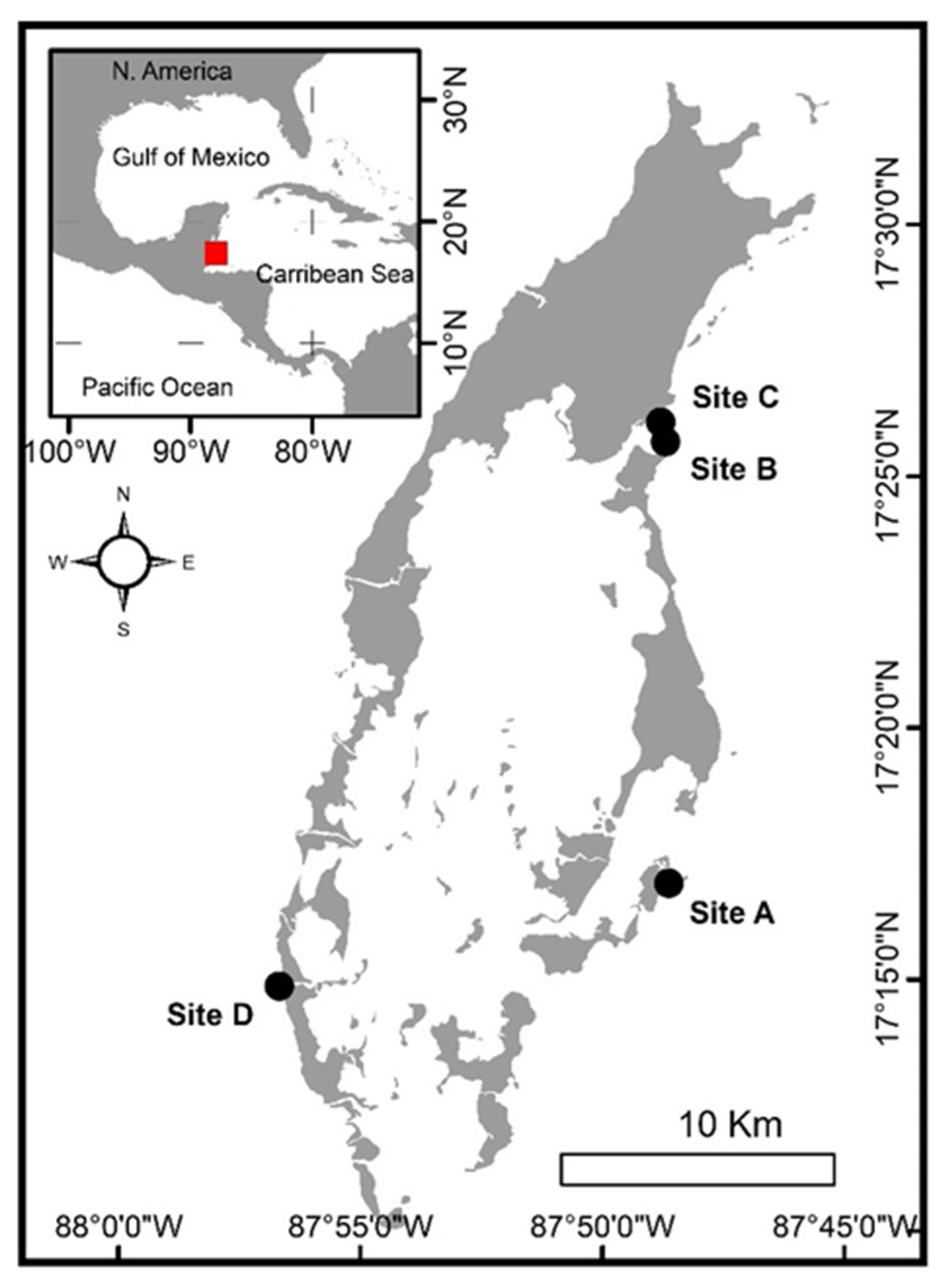
2.1. Study Area
2.2. Survey Methodology
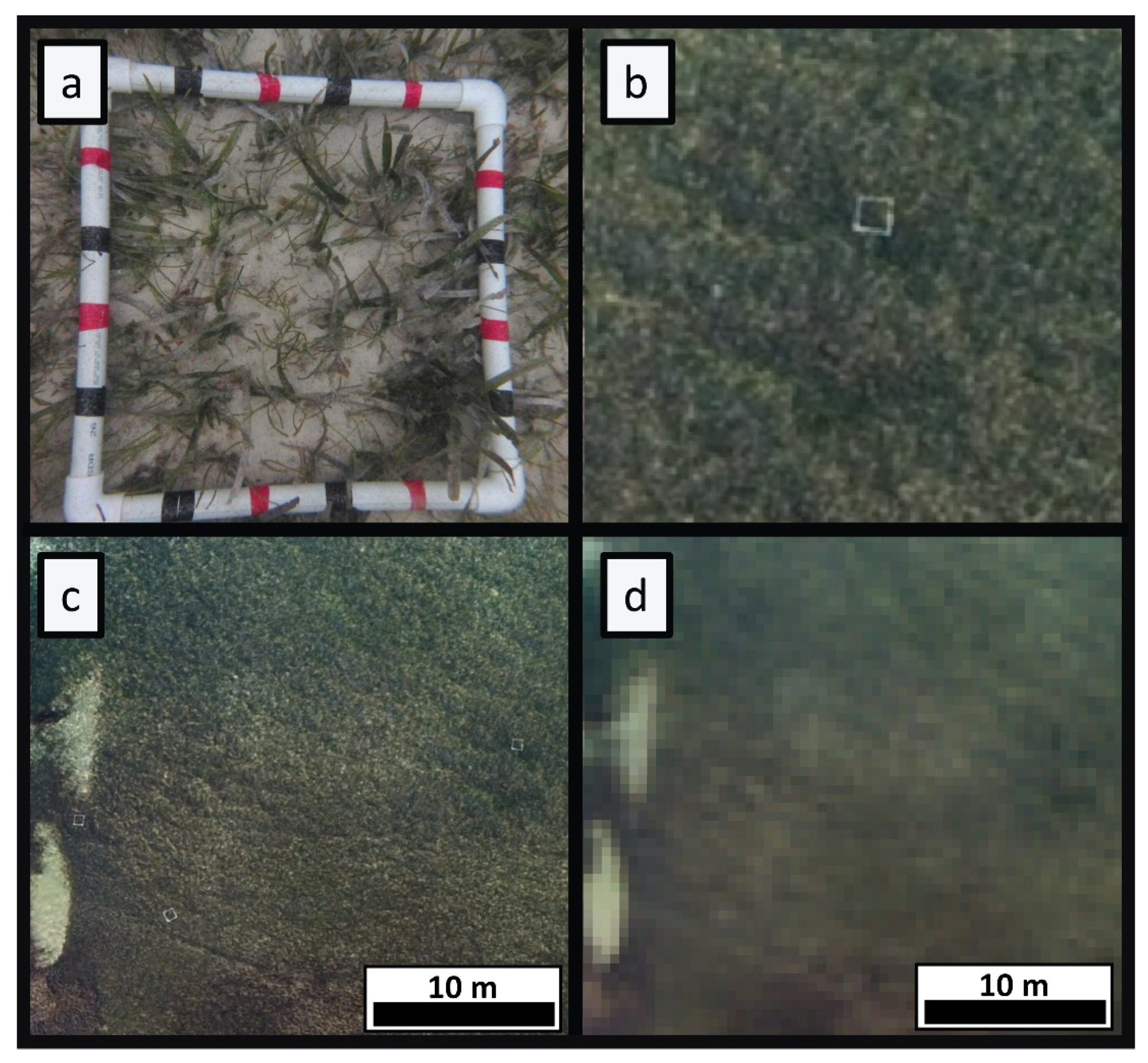
2.3. Ground Truth Data
2.4. Modelling
3. Results
3.1. Flights and Mosaics
3.1.1. Site A
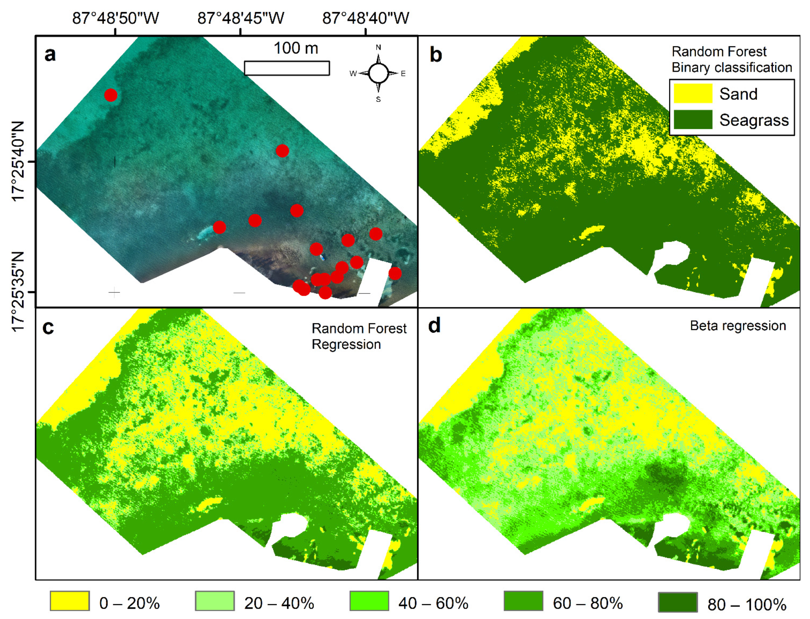
3.1.2. Site B
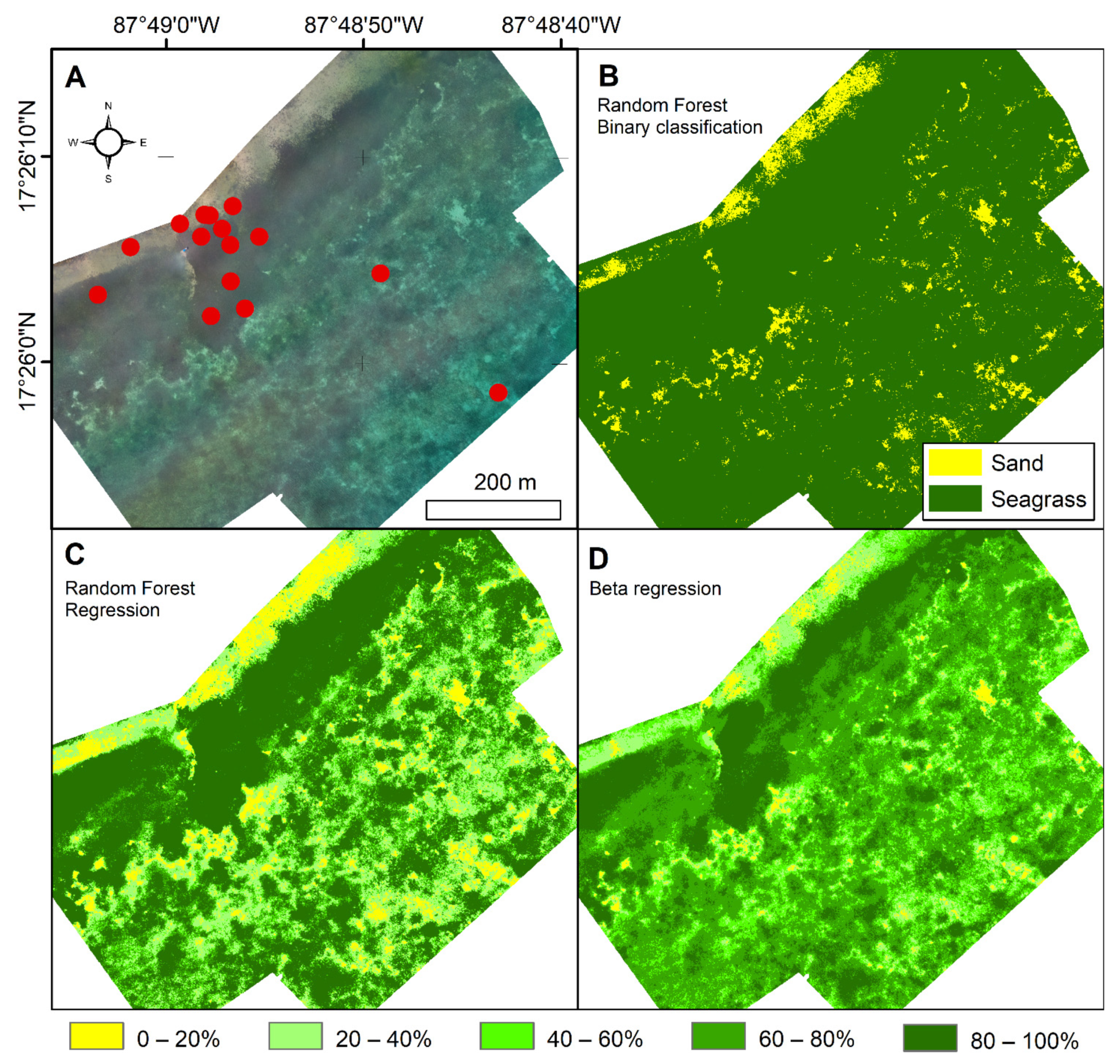
3.1.3. Site C
3.1.4. Site D
3.2. Influence of Modelling
3.3. Seagrass Canopy Cover Predictions
4. Discussion
4.1. Turneffe Atoll Seagrass Beds
4.2. Advances in the Methodology of Mapping Seagrass with UAVs
4.3. Fine-Scale Resolution Mapping in Marine Protected Areas
4.4. Future of Mapping Seagrass Habitats with Drones
5. Conclusions
Supplementary Materials
Author Contributions
Funding
Data Availability Statement
Acknowledgments
Conflicts of Interest
References
- Nagelkerken, I.; Roberts, C.M.; van der Velde, G.; Dorenbosch, M.; van Riel, M.C.; de la Morinere, E.C.; Nienhuis, P.H. How important are mangroves and seagrass beds for coral-reef fish? The nursery hypothesis tested on an island scale. Mar. Ecol. Prog. Ser. 2002, 244, 299–305. [Google Scholar] [CrossRef] [Green Version]
- Dorenbosch, M.; Grol, M.G.G.; Christianen, M.J.A.; Nagelkerken, I.; van der Velde, G. Indo-Pacific seagrass beds and mangroves contribute to fish density coral and diversity on adjacent reefs. Mar. Ecol. Prog. Ser. 2005, 302, 63–76. [Google Scholar] [CrossRef] [Green Version]
- Pau, M. The protection of sandy shores—Can we afford to ignore the contribution of seagrass? Mar. Pollut. Bull. 2018, 134, 152–159. [Google Scholar]
- Christianen, M.J.A.; van Belzen, J.; Herman, P.M.J.; van Katwijk, M.M.; Lamers, L.P.M.; van Leent, P.J.M.; Bouma, T.J. Low-Canopy Seagrass Beds Still Provide Important Coastal Protection Services. PLoS ONE 2013, 8, e26413. [Google Scholar] [CrossRef] [PubMed] [Green Version]
- Attrill, M.J.; Strong, J.A.; Rowden, A.A. Are macroinvertebrate communities influenced by seagrass structural complexity? Ecography 2000, 23, 114–121. [Google Scholar] [CrossRef]
- Duffy, J.E. Biodiversity and the functioning of seagrass ecosystems. Mar. Ecol. Prog. Ser. 2006, 311, 233–250. [Google Scholar] [CrossRef] [Green Version]
- Horinouchi, M. Review of the effects of within-patch scale structural complexity on seagrass fishes. J. Exp. Mar. Biol. Ecol. 2007, 350, 111–129. [Google Scholar] [CrossRef]
- Nordlund, L.M.; Koch, E.W.; Barbier, E.B.; Creed, J.C. Seagrass Ecosystem Services and Their Variability across Genera and Geographical Regions. PLoS ONE 2016, 11, e0163091. [Google Scholar] [CrossRef] [PubMed] [Green Version]
- Mcleod, E.; Chmura, G.L.; Bouillon, S.; Salm, R.; Björk, M.; Duarte, C.M.; Lovelock, C.E.; Schlesinger, W.H.; Silliman, B.R. A blueprint for blue carbon: Toward an improved understanding of the role of vegetated coastal habitats in sequestering CO2. Front. Ecol. Environ 2011, 9, 552–560. [Google Scholar] [CrossRef] [Green Version]
- Fourqurean, J.W.; Duarte, C.M.; Kennedy, H.; Marba, N.; Holmer, M.; Mateo, M.A.; Apostolaki, E.T.; Kendrick, G.A.; Krause-Jensen, D.; McGlathery, K.J.; et al. Seagrass ecosystems as a globally significant carbon stock. Nat. Geosci. 2012, 5, 505–509. [Google Scholar] [CrossRef]
- McCloskey, R.M.; Unsworth, R.K.F. Decreasing seagrass density negatively influences associated fauna. Peerj 2015, 3, 3. [Google Scholar] [CrossRef] [PubMed] [Green Version]
- Whippo, R.; Knight, N.S.; Prentice, C.; Cristiani, J.; Siegle, M.R.; O’Connor, M.I. Epifaunal diversity patterns within and among seagrass meadows suggest landscape-scale biodiversity processes. Ecosphere 2018, 9, e02490. [Google Scholar] [CrossRef] [Green Version]
- Samper-Villarreal, J.; Lovelock, C.E.; Saunders, M.I.; Roelfsema, C.; Mumby, P.J. Organic carbon in seagrass sediments is influenced by seagrass canopy complexity, turbidity, wave height, and water depth. Limnol. Oceanogr. 2016, 61, 938–952. [Google Scholar] [CrossRef] [Green Version]
- Ricart, A.M.; Perez, M.; Romero, J. Landscape configuration modulates carbon storage in seagrass sediments. Estuar. Coast. Shelf Sci. 2017, 185, 69–76. [Google Scholar] [CrossRef]
- Oreska, M.P.J.; McGlathery, K.J.; Porter, J.H. Seagrass blue carbon spatial patterns at the meadow-scale. PLoS ONE 2017, 12, e0176630. [Google Scholar] [CrossRef]
- Mazarrasa, I.; Sarnper-Villarreal, J.; Serrano, O.; Lavery, P.S.; Lovelock, C.E.; Marba, N.; Duarte, C.M.; Cortes, J. Habitat characteristics provide insights of carbon storage in seagrass meadows. Mar. Pollut. Bull. 2018, 134, 106–117. [Google Scholar] [CrossRef]
- Waycott, M.; Duarte, C.M.; Carruthers, T.J.B.; Orth, R.J.; Dennison, W.C.; Olyarnik, S.; Calladine, A.; Fourqurean, J.W.; Heck, K.L.; Hughes, A.R.; et al. Accelerating loss of seagrasses across the globe threatens coastal ecosystems. Proc. Natl. Acad. Sci. USA 2009, 106, 12377–12381. [Google Scholar] [CrossRef] [Green Version]
- Githaiga, M.N.; Frouws, A.M.; Kairo, J.G.; Huxham, M. Seagrass Removal Leads to Rapid Changes in Fauna and Loss of Carbon. Front. Ecol. Evol. 2019, 7, 7. [Google Scholar] [CrossRef] [Green Version]
- Phinn, S.; Roelfsema, C.; Dekker, A.; Brando, V.; Anstee, J. Mapping seagrass species, cover and biomass in shallow waters: An assessment of satellite multi-spectral and airborne hyper-spectral imaging systems in Moreton Bay (Australia). Remote Sens. Environ. 2008, 112, 3413–3425. [Google Scholar] [CrossRef]
- Topouzelis, K.; Makri, D.; Stoupas, N.; Papakonstantinou, A.; Katsanevakis, S. Seagrass mapping in Greek territorial waters using Landsat-8 satellite images. Int. J. Appl. Earth Obs. 2018, 67, 98–113. [Google Scholar] [CrossRef]
- Hossain, M.S.; Bujang, J.S.; Zakaria, M.H.; Hashim, M. The application of remote sensing to seagrass ecosystems: An overview and future research prospects. Int. J. Remote Sens. 2015, 36, 61–114. [Google Scholar] [CrossRef]
- Lo Iacono, C.; Mateo, M.A.; Gracia, E.; Guasch, L.; Carbonell, R.; Serrano, L.; Serrano, O.; Danobeitia, J. Very high-resolution seismo-acoustic imaging of seagrass meadows (Mediterranean Sea): Implications for carbon sink estimates. Geophys. Res. Lett. 2008, 35, 5. [Google Scholar] [CrossRef]
- Micallef, A.; Le Bas, T.P.; Huvenne, V.A.I.; Blondel, P.; Huhnerbach, V.; Deidun, A. A multi-method approach for benthic habitat mapping of shallow coastal areas with high-resolution multibeam data. Cont. Shelf Res. 2012, 39, 14–26. [Google Scholar] [CrossRef] [Green Version]
- Greene, A.; Rahman, A.F.; Kline, R.; Rahman, M.S. Side scan sonar: A cost-efficient alternative method for measuring seagrass cover in shallow environments. Estuar Coast. Shelf Sci. 2018, 207, 250–258. [Google Scholar] [CrossRef]
- Tyllianakis, E.; Callaway, A.; Vanstaen, K.; Luisetti, T. The value of information: Realising the economic benefits of mapping seagrass meadows in the British Virgin Islands. Sci. Total Environ. 2019, 650, 2107–2116. [Google Scholar] [CrossRef]
- Rende, S.F.; Bosman, A.; Di Mento, R.; Bruno, F.; Lagudi, A.; Irving, A.D.; Dattola, L.; Di Giambattista, L.; Lanera, P.; Proietti, R.; et al. Ultra-High-Resolution Mapping of Posidonia oceanica (L.) Delile Meadows through Acoustic, Optical Data and Object-based Image Classification. J. Mar. Sci. Eng. 2020, 8, 647. [Google Scholar] [CrossRef]
- Rende, F.S.; Irving, A.D.; Lagudi, A.; Bruno, F.; Scalise, S.; Cappa, P.; Montefalcone, M.; Bacci, T.; Penna, M.; Trabucco, B.; et al. Pilot Application of 3d Underwater Imaging Techniques for Mapping Posidonia oceanica (L.) Delile Meadows. Int. Arch. Photogramm. 2015, 45, 177–181. [Google Scholar]
- Rende, S.F.; Irving, A.D.; Bacci, T.; Parlagreco, L.; Bruno, F.; De Filippo, F.; Montefalcone, M.; Penna, M.; Trabucco, B.; Di Mento, R.; et al. Advances in micro-cartography: A two-dimensional photo mosaicing technique for seagrass monitoring. Estuar. Coast Shelf Sci. 2015, 167, 475–486. [Google Scholar] [CrossRef]
- Scardi, M.; Chessa, L.A.; Fresi, E.; Pais, A.; Serra, S. Optimizing interpolation of shoot density data from a Posidonia oceanica seagrass bed. Mar. Ecol. 2006, 27, 339–349. [Google Scholar] [CrossRef] [Green Version]
- Chauvaud, S.; Bouchon, C.; Maniere, R. Remote sensing techniques adapted to high resolution mapping of tropical coastal marine ecosystems (coral reefs, seagrass beds and mangrove). Int. J. Remote Sens. 1998, 19, 3625–3639. [Google Scholar] [CrossRef]
- Kendrick, G.A.; Aylward, M.J.; Hegge, B.J.; Cambridge, M.L.; Hillman, K.; Wyllie, A.; Lord, D.A. Changes in seagrass coverage in Cockburn Sound, Western Australia between 1967 and 1999. Aquat. Bot. 2002, 73, 75–87. [Google Scholar] [CrossRef]
- Murdoch, T.J.T.; Glasspool, A.F.; Outerbridge, M.; Ward, J.; Manuel, S.; Gray, J.; Nash, A.; Coates, K.A.; Pitt, J.; Fourqurean, J.W.; et al. Large-scale decline in offshore seagrass meadows in Bermuda. Mar. Ecol. Prog. Ser. 2007, 339, 123–130. [Google Scholar] [CrossRef] [Green Version]
- Duffy, J.P.; Pratt, L.; Anderson, K.; Land, P.E.; Shutler, J.D. Spatial assessment of intertidal seagrass meadows using optical imaging systems and a lightweight drone. Estuar. Coast. Shelf Sci. 2018, 200, 169–180. [Google Scholar] [CrossRef]
- Veettil, B.K.; Ward, R.D.; Lima, M.D.A.C.; Stankovic, M.; Hoai, P.N.; Quang, N.X. Opportunities for seagrass research derived from remote sensing: A review of current methods. Ecol. Indic. 2020, 117, 106560. [Google Scholar] [CrossRef]
- Ventura, D.; Bruno, M.; Lasinio, G.J.; Belluscio, A.; Ardizzone, G. A low-cost drone based application for identifying and mapping of coastal fish nursery grounds. Estuar. Coast. Shelf Sci. 2016, 171, 85–98. [Google Scholar] [CrossRef]
- Chen, J.; Sasaki, J. Mapping of Subtidal and Intertidal Seagrass Meadows via Application of the Feature Pyramid Network to Unmanned Aerial Vehicle Orthophotos. Remote Sens. 2021, 13, 4880. [Google Scholar] [CrossRef]
- Ventura, D.; Bonifazi, A.; Gravina, M.F.; Belluscio, A.; Ardizzone, G. Mapping and Classification of Ecologically Sensitive Marine Habitats Using Unmanned Aerial Vehicle (UAV) Imagery and Object-Based Image Analysis (OBIA). Remote Sens. 2018, 10, 1331. [Google Scholar] [CrossRef] [Green Version]
- Nahirnick, N.K.; Reshitnyk, L.; Campbell, M.; Hessing-Lewis, M.; Costa, M.; Yakimishyn, J.; Lee, L. Mapping with confidence; delineating seagrass habitats using Unoccupied Aerial Systems (UAS). Remote Sens. Ecol. Con. 2019, 5, 121–135. [Google Scholar] [CrossRef]
- Ellis, S.L.; Taylor, M.L.; Schiele, M.; Letessier, T.B. Influence of altitude on tropical marine habitat classification using imagery from fixed-wing, water-landing UAVs. Remote Sens. Ecol. Con. 2021, 7, 50–63. [Google Scholar] [CrossRef]
- Papakonstantinou, A.; Stamati, C.; Topouzelis, K. Comparison of True-Color and Multispectral Unmanned Aerial Systems Imagery for Marine Habitat Mapping Using Object-Based Image Analysis. Remote Sens. 2020, 12, 554. [Google Scholar] [CrossRef] [Green Version]
- Roelfsema, C.M.; Lyons, M.; Kovacs, E.M.; Maxwell, P.; Saunders, M.I.; Samper-Villarreal, J.; Phinn, S.R. Multi-temporal mapping of seagrass cover, species and biomass: A semi-automated object based image analysis approach. Remote Sens. Environ. 2014, 150, 172–187. [Google Scholar] [CrossRef]
- Fedler, T. The Value of Turneffe Atoll Mangrove Forests, Seagrass Beds and Coral Reefs in Protecting Belize City from Storms. 2018. Available online: https://www.turneffeatoll.org/app/webroot/userfiles/66/File/Turneffe%20Storm%20Mitigation%20Value%20Report%20FINAL.pdf (accessed on 28 November 2021).
- Coastal Zone Management Authority and Institute (CZMAI). Belize Integrated Coastal Zone Management Plan; CZMAI: Belize City, Belize, 2016. [Google Scholar]
- Casella, E.; Collin, A.; Harris, D.; Ferse, S.; Bejarano, S.; Parravicini, V.; Hench, J.L.; Rovere, A. Mapping coral reefs using consumer-grade drones and structure from motion photogrammetry techniques. Coral. Reefs. 2017, 36, 269–275. [Google Scholar] [CrossRef]
- Turner, D.; Lucieer, A.; Watson, C. An Automated Technique for Generating Georectified Mosaics from Ultra-High Resolution Unmanned Aerial Vehicle (UAV) Imagery, Based on Structure from Motion (SfM) Point Clouds. Remote Sens. 2012, 4, 1392–1410. [Google Scholar] [CrossRef] [Green Version]
- Pfeifer, N.; Glira, P.; Briese, C. Direct Georeferencing with on Board Navigation Components of Light Weight Uav Platforms. Xxii Isprs. Congr. Tech. Comm. Vii 2012, 39, 487–492. [Google Scholar] [CrossRef] [Green Version]
- Joyce, K.E.; Duce, S.; Leahy, S.M.; Leon, J.; Maier, S.W. Principles and practice of acquiring drone-based image data in marine environments. Mar. Freshw. Res. 2019, 70, 952–963. [Google Scholar] [CrossRef]
- Gauci, A.A.; Brodbeck, C.J.; Poncet, A.M.; Knappenberger, T. Assessing the geospatial accuracy of aerial imagery collected with various UAS platforms. Trans. ASABE 2018, 61, 1823–1829. [Google Scholar] [CrossRef]
- Woodget, A. Quantifying Physical River Habitat Parametres Using Hyperspatial Resolution UAS Imagery and SfM-Photogrammetry; University of Worcester: Worcester, UK, 2015. [Google Scholar]
- Murfitt, S.L.; Allan, B.M.; Bellgrove, A.; Rattray, A.; Young, M.A.; Ierodiaconou, D. Applications of unmanned aerial vehicles in intertidal reef monitoring. Sci Rep. 2017, 7, 10259. [Google Scholar] [CrossRef] [Green Version]
- Ferrari, S.L.P.; Cribari-Neto, F. Beta regression for modelling rates and proportions. J. Appl. Stat. 2004, 31, 799–815. [Google Scholar] [CrossRef]
- Coulston, J.W.; Moisen, G.G.; Wilson, B.T.; Finco, M.V.; Cohen, W.B.; Brewer, C.K. Modeling Percent Tree Canopy Cover: A Pilot Study. Photogramm. Eng. Remote Sens. 2012, 78, 715–727. [Google Scholar] [CrossRef] [Green Version]
- Korhonen, L.; Korhonen, K.T.; Stenberg, P.; Maltamo, M.; Rautiainen, M. Local models for forest canopy cover with beta regression. Silva. Fenn. 2007, 41, 671–685. [Google Scholar] [CrossRef] [Green Version]
- Liaw, A.; Wiener, M. Classification and regression by randomForest. R News 2002, 2, 18–22. [Google Scholar]
- Kendrick, G.A.; Holmes, K.W.; Van Niel, K.P. Multi-scale spatial patterns of three seagrass species with different growth dynamics. Ecography 2008, 31, 191–200. [Google Scholar] [CrossRef]
- Van der Heide, T.; Bouma, T.J.; van Nes, E.H.; van de Koppel, J.; Scheffer, M.; Roelofs, J.G.M.; van Katwijk, M.M.; Smolders, A.J.P. Spatial self-organized patterning in seagrasses along a depth gradient of an intertidal ecosystem. Ecology 2010, 91, 362–369. [Google Scholar] [CrossRef] [PubMed] [Green Version]
- Ariasari, A.; Hartono; Wicaksono, P. Random Forest Classification and Regression for Seagrass Mapping using PlanetScope Image in Labuan Bajo, East Nusa Tenggara. Proc. SPIE 2019, 11372, 113721Q. [Google Scholar]
- Fauzan, M.A.; Kumara, I.S.W.; Yogyantoro, R.; Suwardana, S.; Fadhilah, N.; Nurmalasari, I.; Apriyani, S.; Wicaksono, P. Assessing the capability of Sentinel-2A data for mapping seagrass percent cover in Jerowaru, East Lombok. Indones. J. Geogr. 2017, 49, 195–203. [Google Scholar] [CrossRef] [Green Version]
- Roelfsema, C.; Kovacs, E.M.; Saunders, M.I.; Phinn, S.; Lyons, M.; Maxwell, P. Challenges of remote sensing for quantifying changes in large complex seagrass environments. Estuar. Coast. Shelf Sci. 2013, 133, 161–171. [Google Scholar] [CrossRef]
- Government of Belize Press Office. Expansion of Fisheries Replenishment (No-Take) Zones. Available online: https://www.pressoffice.gov.bz/expansion-of-fisheries-replenishment-no-take-zones/ (accessed on 28 November 2021).
- Government of Belize Press Office. Expansion of the Sapodilla Cayes Marine Reserve to Protect Important Reef Ecosystem. Available online: https://www.pressoffice.gov.bz/expansion-of-the-sapodilla-cayes-marine-reserve-to-protect-important-reef-ecosystem/ (accessed on 28 November 2021).
- Congdon, V.M.; Wilson, S.S.; Dunton, K.H. Evaluation of Relationships Between Cover Estimates and Biomass in Subtropical Seagrass Meadows and Application to Landscape Estimates of Carbon Storage. Southeast Geogr. 2017, 57, 231–245. [Google Scholar] [CrossRef]
- Mallombasi, A.; Mashoreng, S.; La Nafie, Y.A. The relationship between seagrass Thalassia hemprichii percentage cover and their biomass. J. Ilmu Kelaut. SPERMONDE 2020, 6, 7–10. [Google Scholar] [CrossRef]
- Duarte, C.M.; Marbà, N.; Gacia, E.; Fourqurean, J.W.; Beggins, J.; Barrón, C.; Apostolaki, E.T. Seagrass community metabolism: Assessing the carbon sink capacity of seagrass meadows. Glob. Biogeochem. Cycles 2010, 24, 1–8. [Google Scholar] [CrossRef] [Green Version]
- Fonseca, M.S.; Bell, S.S. Influence of physical setting on seagrass landscapes near Beaufort, North Carolina, USA. Mar. Ecol. Prog. Ser. 1998, 171, 109–121. [Google Scholar] [CrossRef] [Green Version]
- Downie, A.L.; von Numers, M.; Boström, C. Influence of model selection on the predicted distribution of the seagrass Zostera marina. Estuar. Coast. Shelf Sci. 2013, 121, 8–19. [Google Scholar] [CrossRef]
- Carpenter, S.; Byfield, V.; Felgate, S.; Price, D.; Andrade, V.; Cobb, E.; Strong, J.; Lichtschlag, A.; Brittain, H.; Barry, C.; et al. Using Unoccupied Aerial Vehicles (UAVs) to Map Seagrass Cover from Sentinel-2 imagery. Remote Sens. 2022, 14, 477. [Google Scholar] [CrossRef]
- Fallati, L.; Saponari, L.; Savini, A.; Marchese, F.; Corselli, C.; Galli, P. Multi-Temporal UAV Data and Object-Based Image Analysis (OBIA) for Estimation of Substrate Changes in a Post-Bleaching Scenario on a Maldivian Reef. Remote Sens. 2020, 12, 2093. [Google Scholar] [CrossRef]
- Yang, B.; Hawthorne, T.L.; Hessing-Lewis, M.; Duffy, E.J.; Reshitnyk, L.Y.; Feinman, M.; Searson, H. Developing an Introductory UAV/Drone Mapping Training Program for Seagrass Monitoring and Research. Drones 2020, 4, 70. [Google Scholar] [CrossRef]
- Sanz-Ablanedo, E.; Chandler, J.H.; Ballesteros-Pérez, P.; Rodríguez-Pérez, J.R. Reducing systematic dome errors in digital elevation models through better UAV flight design. Earth Surf. Process. Landf. 2020, 45, 2134–2147. [Google Scholar] [CrossRef]
- Lesser, M.P.; Mobley, C.D. Bathymetry, water optical properties, and benthic classification of coral reefs using hyperspectral remote sensing imagery. Coral. Reefs. 2007, 26, 819–829. [Google Scholar] [CrossRef]
- Bajjouk, T.; Mouquet, P.; Ropert, M.; Quod, J.P.; Hoarau, L.; Bigot, L.; Le Dantec, N.; Delacourt, C.; Populus, J. Detection of changes in shallow coral reefs status: Towards a spatial approach using hyperspectral and multispectral data. Ecol. Indic. 2019, 96, 174–191. [Google Scholar] [CrossRef]
- Rossiter, T.; Furey, T.; McCarthy, T.; Stengel, D.B. UAV-mounted hyperspectral mapping of intertidal macroalgae. Estuar. Coast. Shelf Sci. 2020, 242, 106789. [Google Scholar] [CrossRef]
- James, D.; Collin, A.; Houet, T.; Mury, A.; Gloria, H.; Le Poulain, N. Towards Better Mapping of Seagrass Meadows using UAV Multispectral and Topographic Data. J. Coast. Res. 2020, 95, 1117–1121. [Google Scholar] [CrossRef]
- Hochberg, E.J.; Andréfouët, S.; Tyler, M.R. Sea surface correction of high spatial resolution Ikonos images to improve bottom mapping in near-shore environments. IEEE Trans. Geosci. Remote Sens. 2003, 41, 1724–1729. [Google Scholar] [CrossRef]
- Cavanaugh, K.C.; Cavanaugh, K.C.; Bell, T.W.; Hockridge, E.G. An automated method for mapping giant kelp canopy dynamics from UAV. Front. Environ. Sci. 2021, 8, 301. [Google Scholar] [CrossRef]
- Chirayath, V.; Earle, S.A. Drones that see through waves—Preliminary results from airborne fluid lensing for centimetre-scale aquatic conservation. Aquat. Conserv. 2016, 26, 237–250. [Google Scholar] [CrossRef] [Green Version]
- Chirayath, V.; Instrella, R. Fluid lensing and machine learning for centimeter-resolution airborne assessment of coral reefs in American Samoa. Remote Sens. Environ. 2019, 235, 111475. [Google Scholar] [CrossRef]


| Location | Date | Time | Number of Flights | Number of Images Collected | Number of Images Utilised | Flight Altitude | Area of Orthomosaic Used in Analysis (ha) |
|---|---|---|---|---|---|---|---|
| Site A | 22 January 2019 | 16:00 | 1 | 66 | 66 | 100 | 8.49 |
| Site B | 24 January 2019 | 16:27 | 1 | 128 | 123 | 80 | 8.6 |
| Site C | 25 January 2019 | 16:08 | 2 | 418 | 338 | 80 | 43.73 |
| Site D | 26 January 2019 | 16:05 | 2 | 396 | 273 | 80 | 11.66 |
| Class Area Predicted from the Random Forest (Regression) Model (m2) | Class Area Predicted from the Beta Regression Model (m2) | |||||||
|---|---|---|---|---|---|---|---|---|
| Seagrass (% Cover) | Site A | Site B | Site C | Site D | Site A | Site B | Site C | Site D |
| 0–20 | 7834 | 23,625 | 35,434 | 17,594 | 5676 | 22,654 | 10,023 | 7821 |
| 20–40 | 6380 | 12,525 | 92,957 | 2045 | 3892 | 25,703 | 40,195 | 11,939 |
| 40–60 | 4858 | 7604 | 43,270 | 1451 | 7332 | 21,526 | 87,558 | 12,924 |
| 60–80 | 11,662 | 40,639 | 77,172 | 2756 | 21,654 | 12,873 | 199,159 | 50,997 |
| 80–100 | 54,182 | 1567 | 188,480 | 92,785 | 46,362 | 3205 | 100,379 | 32,949 |
| Class | Class area (m2) predicted from the Random Forest (binary) model | |||||||
| Seagrass | 77,075 | 71,098 | 411,614 | 100,537 | ||||
| Sand | 7840 | 14,862 | 25,700 | 16,094 | ||||
| Variance Explained (%) | Pseudo R2 | Out of Bag Error (%) | Adjusted R2 | Adjusted R2 | ||
|---|---|---|---|---|---|---|
| Train | Test | Test Data (Exc. Post Hoc) | ||||
| Random Forest classification | 8.77 | |||||
| Random Forest | 94.15 | 0.98 | 0.91 | 0.76 | ||
| Beta regression | 0.75 | 0.92 | 0.91 | 0.67 | ||
Publisher’s Note: MDPI stays neutral with regard to jurisdictional claims in published maps and institutional affiliations. |
© 2022 by the authors. Licensee MDPI, Basel, Switzerland. This article is an open access article distributed under the terms and conditions of the Creative Commons Attribution (CC BY) license (https://creativecommons.org/licenses/by/4.0/).
Share and Cite
Price, D.M.; Felgate, S.L.; Huvenne, V.A.I.; Strong, J.; Carpenter, S.; Barry, C.; Lichtschlag, A.; Sanders, R.; Carrias, A.; Young, A.; et al. Quantifying the Intra-Habitat Variation of Seagrass Beds with Unoccupied Aerial Vehicles (UAVs). Remote Sens. 2022, 14, 480. https://doi.org/10.3390/rs14030480
Price DM, Felgate SL, Huvenne VAI, Strong J, Carpenter S, Barry C, Lichtschlag A, Sanders R, Carrias A, Young A, et al. Quantifying the Intra-Habitat Variation of Seagrass Beds with Unoccupied Aerial Vehicles (UAVs). Remote Sensing. 2022; 14(3):480. https://doi.org/10.3390/rs14030480
Chicago/Turabian StylePrice, David M., Stacey L. Felgate, Veerle A. I. Huvenne, James Strong, Stephen Carpenter, Chris Barry, Anna Lichtschlag, Richard Sanders, Abel Carrias, Arlene Young, and et al. 2022. "Quantifying the Intra-Habitat Variation of Seagrass Beds with Unoccupied Aerial Vehicles (UAVs)" Remote Sensing 14, no. 3: 480. https://doi.org/10.3390/rs14030480
APA StylePrice, D. M., Felgate, S. L., Huvenne, V. A. I., Strong, J., Carpenter, S., Barry, C., Lichtschlag, A., Sanders, R., Carrias, A., Young, A., Andrade, V., Cobb, E., Le Bas, T., Brittain, H., & Evans, C. (2022). Quantifying the Intra-Habitat Variation of Seagrass Beds with Unoccupied Aerial Vehicles (UAVs). Remote Sensing, 14(3), 480. https://doi.org/10.3390/rs14030480