


Surface Albedo and Snowline Altitude Estimation Using Optical Satellite Imagery and In Situ Measurements in Muz Taw Glacier, Sawir Mountains

Abstract
1. Introduction
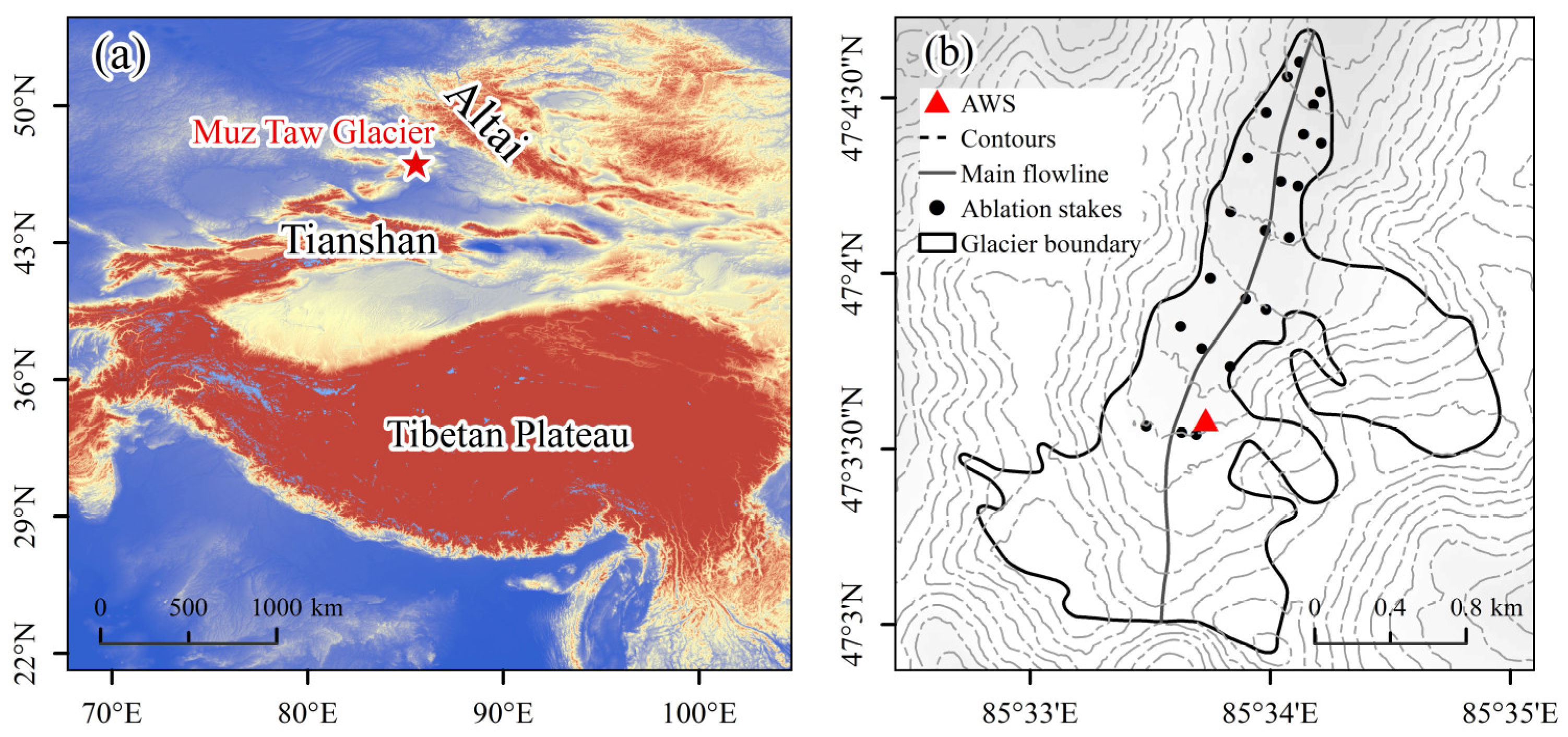
2. Study Area
3. Data and Methods
3.1. Data Sources
3.1.1. Remote Sensing Data
3.1.2. In Situ Measurements
3.1.3. Meteorological Data from ERA-5
3.2. Methods and Data Processing
3.2.1. The Glacier Surface Albedo Derived from Landsat and MOD10A1
3.2.2. Snowline Altitude Extraction
4. Results and Analyses
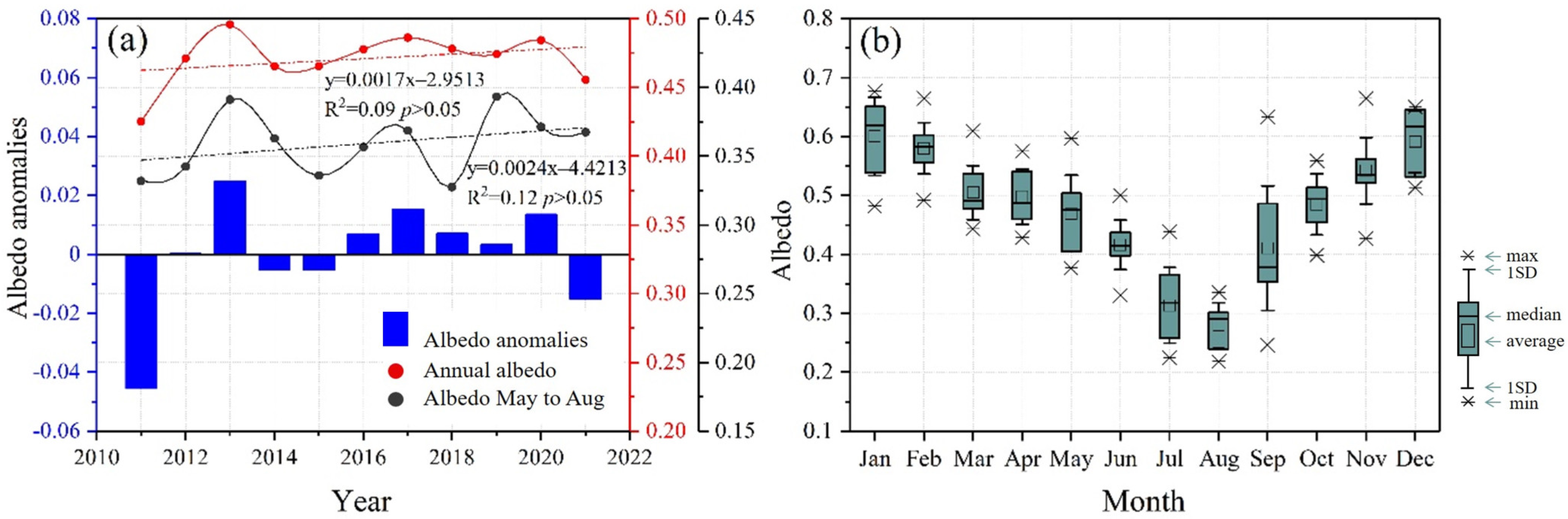
4.1. Long-Term Variation of Glacier Surface Albedo
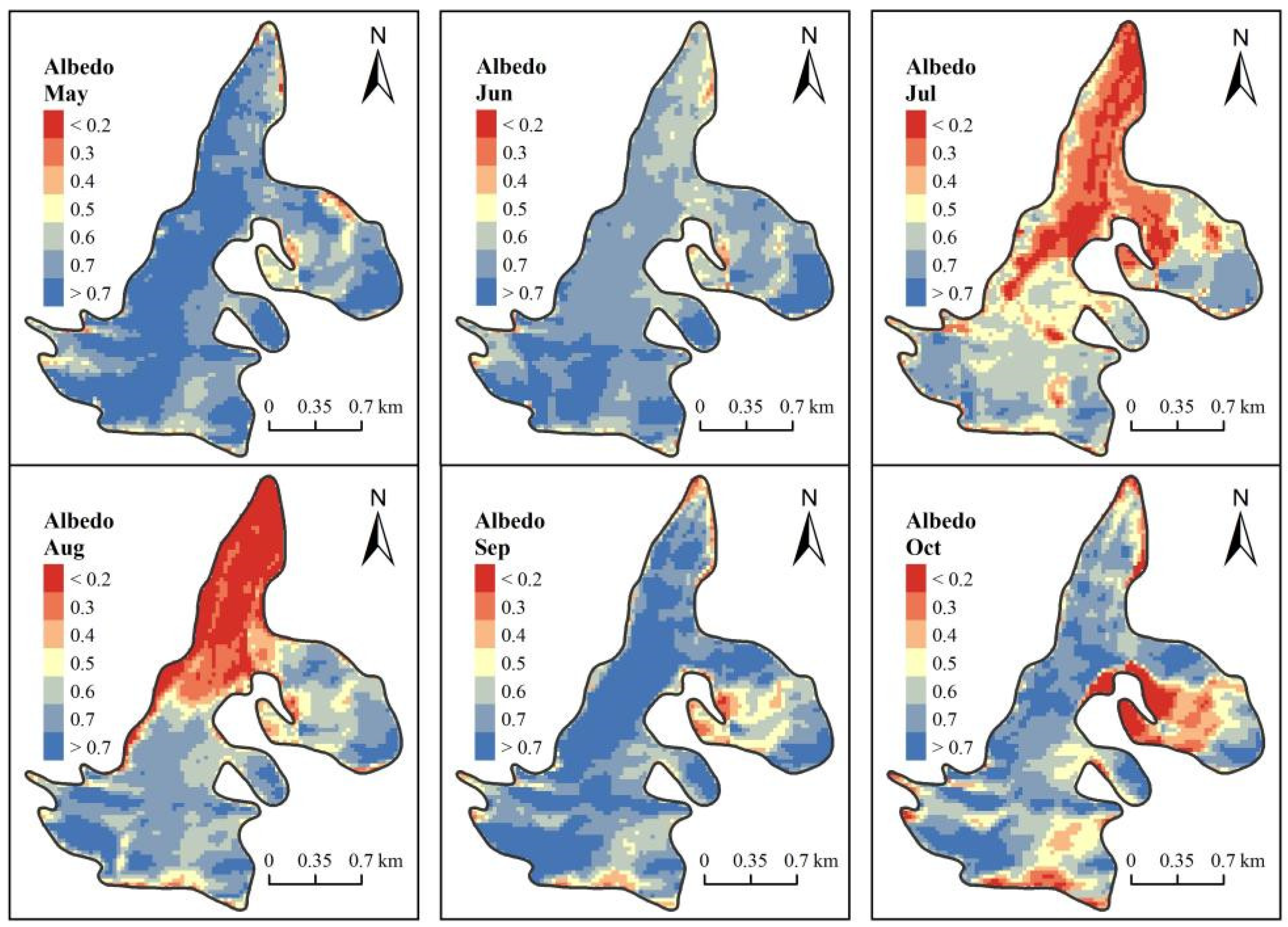
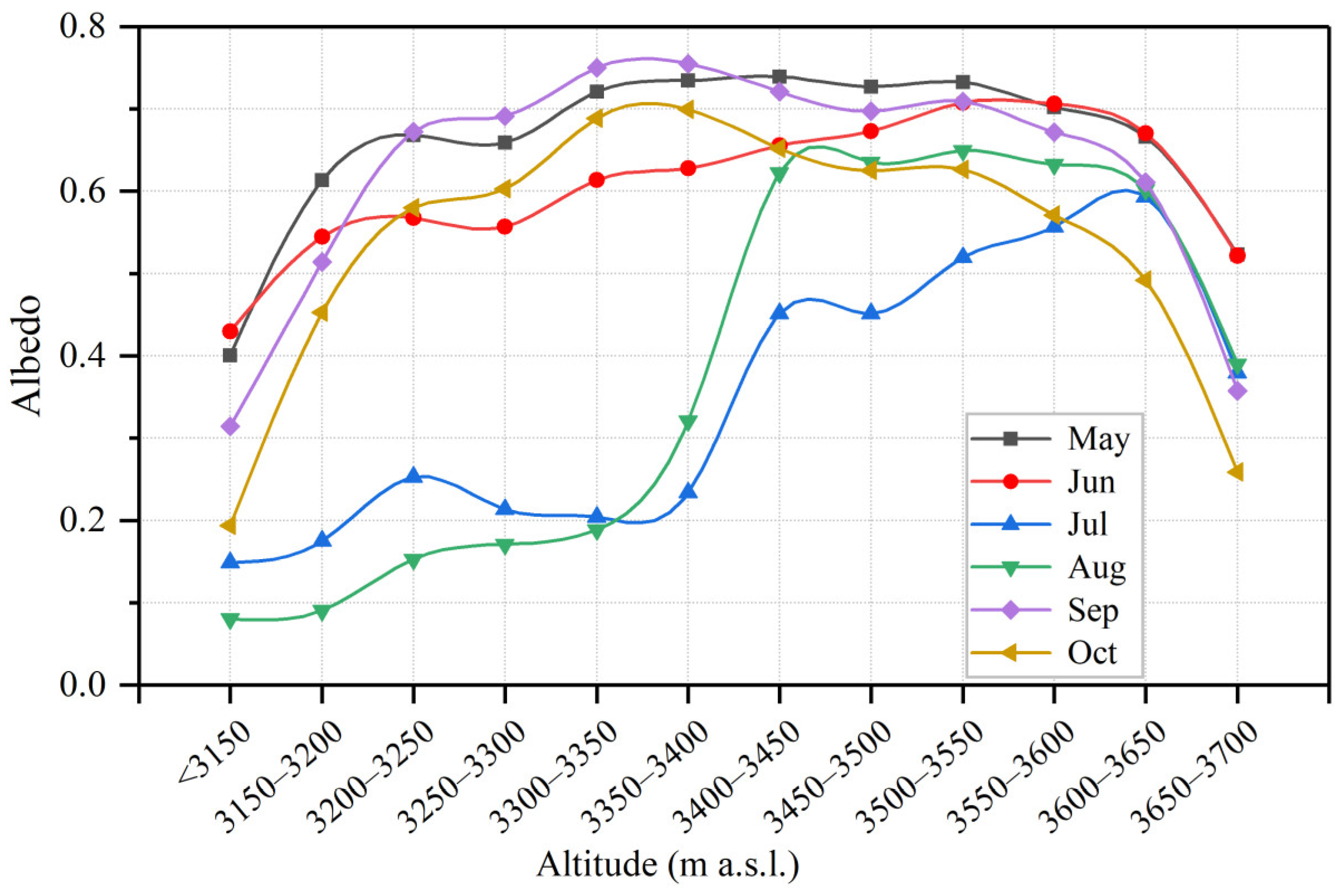
4.2. Multi-Scale Variability of Glacier Surface Albedo
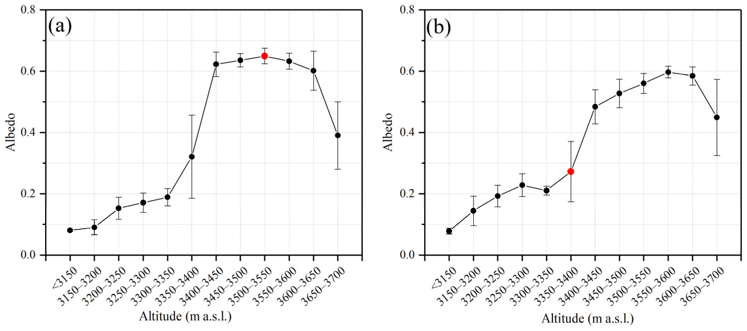
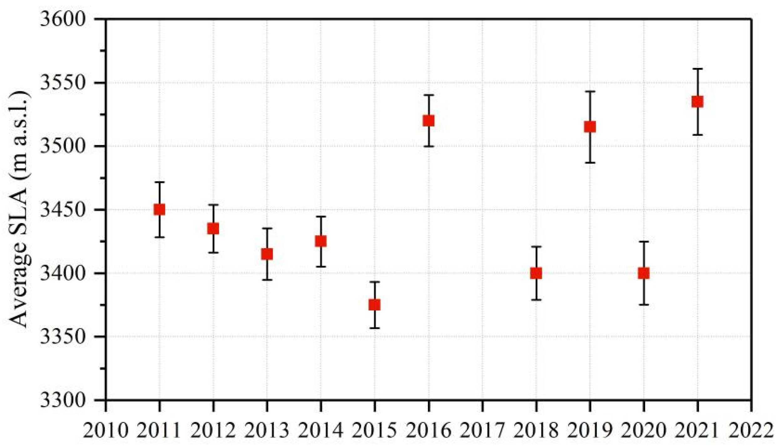
4.3. Variability of Glacier Snowline Altitude
5. Discussion
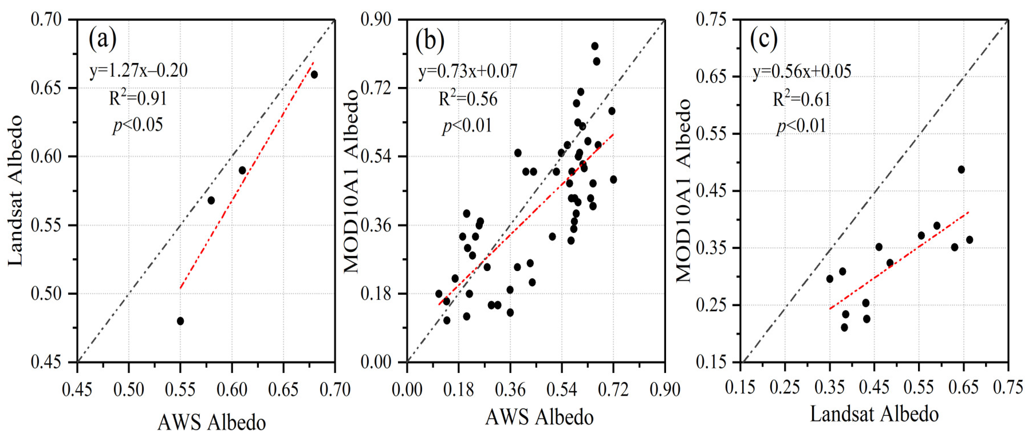
5.1. Uncertainty Estimation of Glacier Surface Albedo
5.2. Uncertainty Estimation of Glacier Snowline Altitude
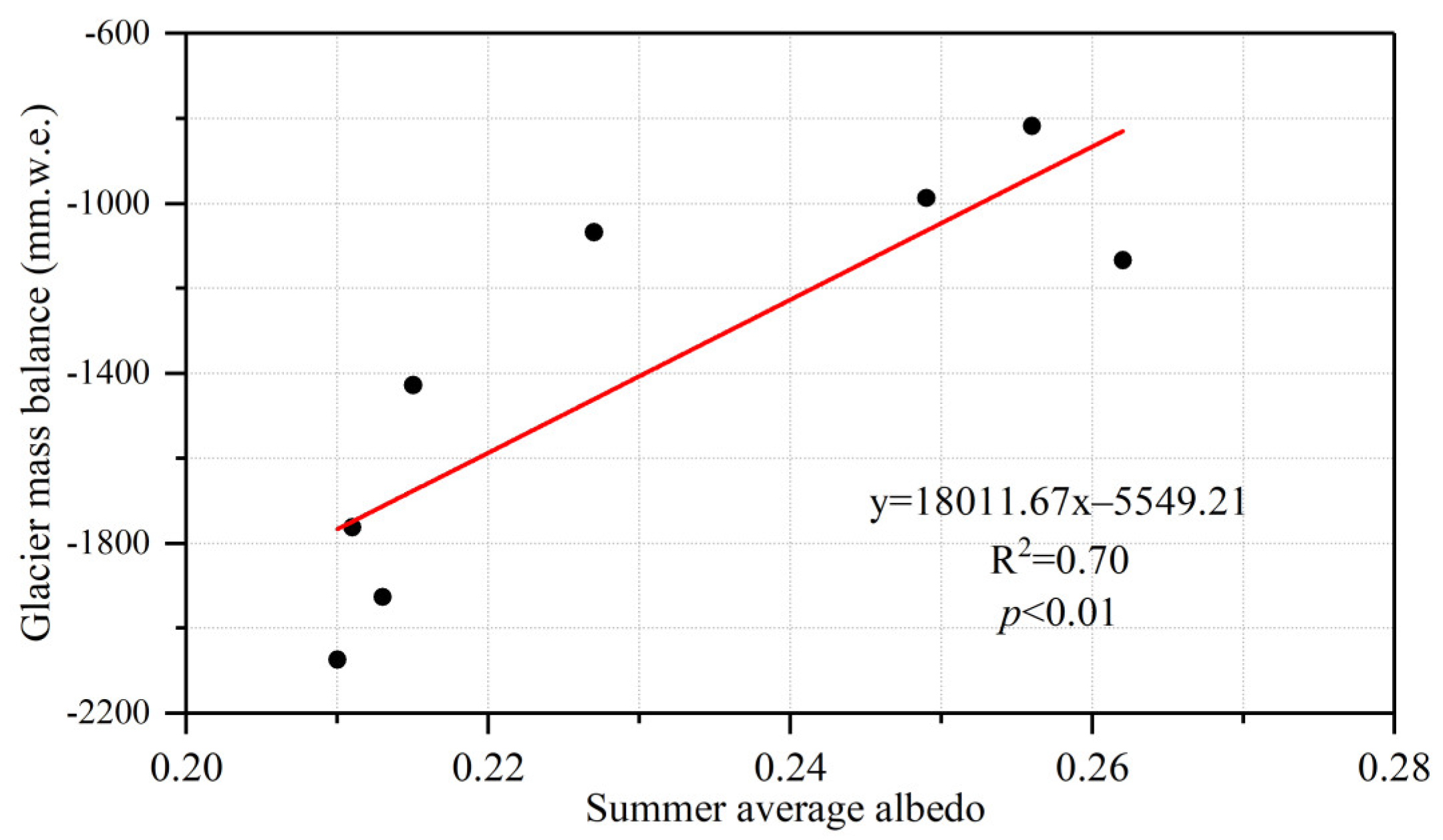
5.3. Potential Impact of Albedo Variation on Glacier Melt
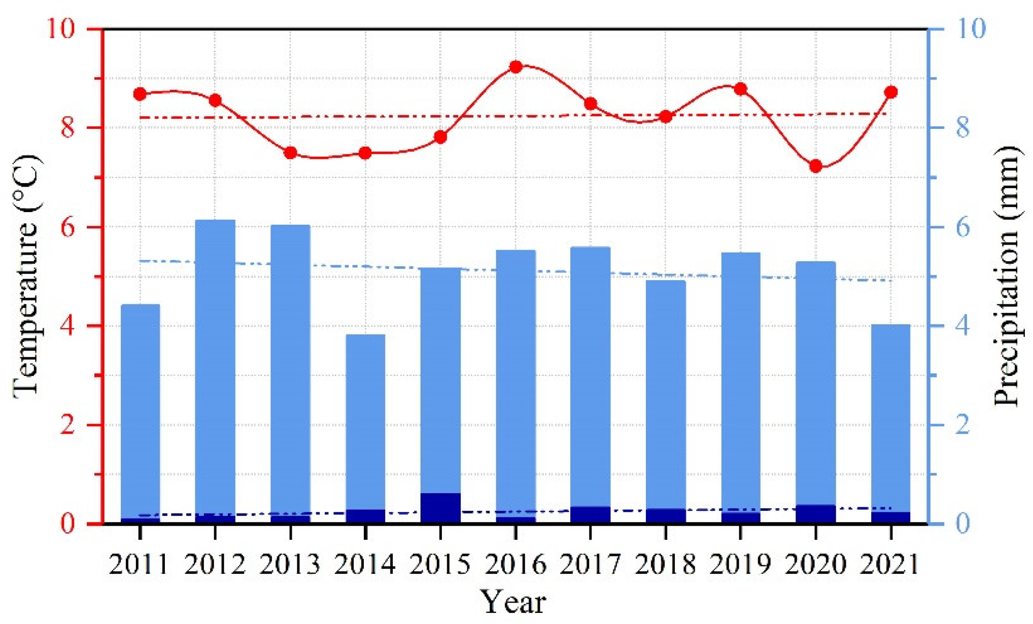
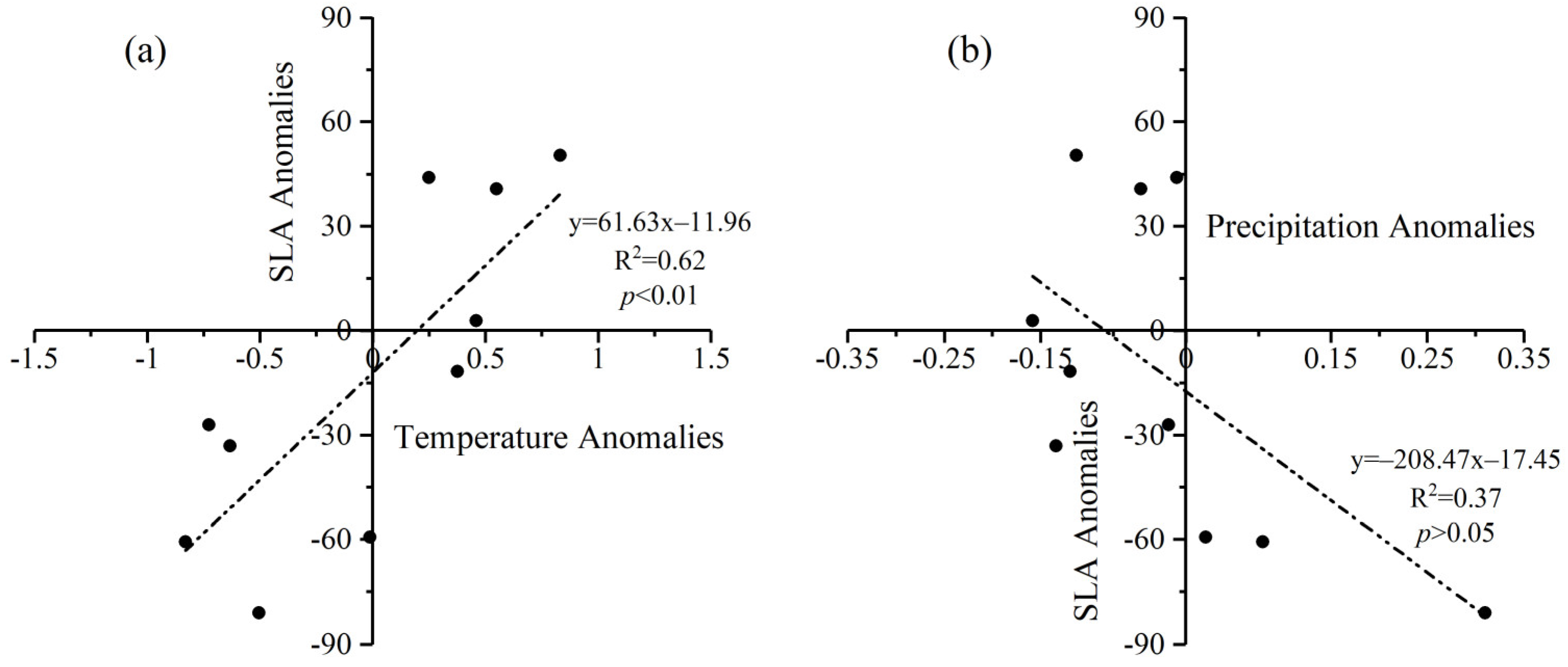
5.4. The Impact of Air Temperature and Precipitation Variation on Snowline Altitude Changes
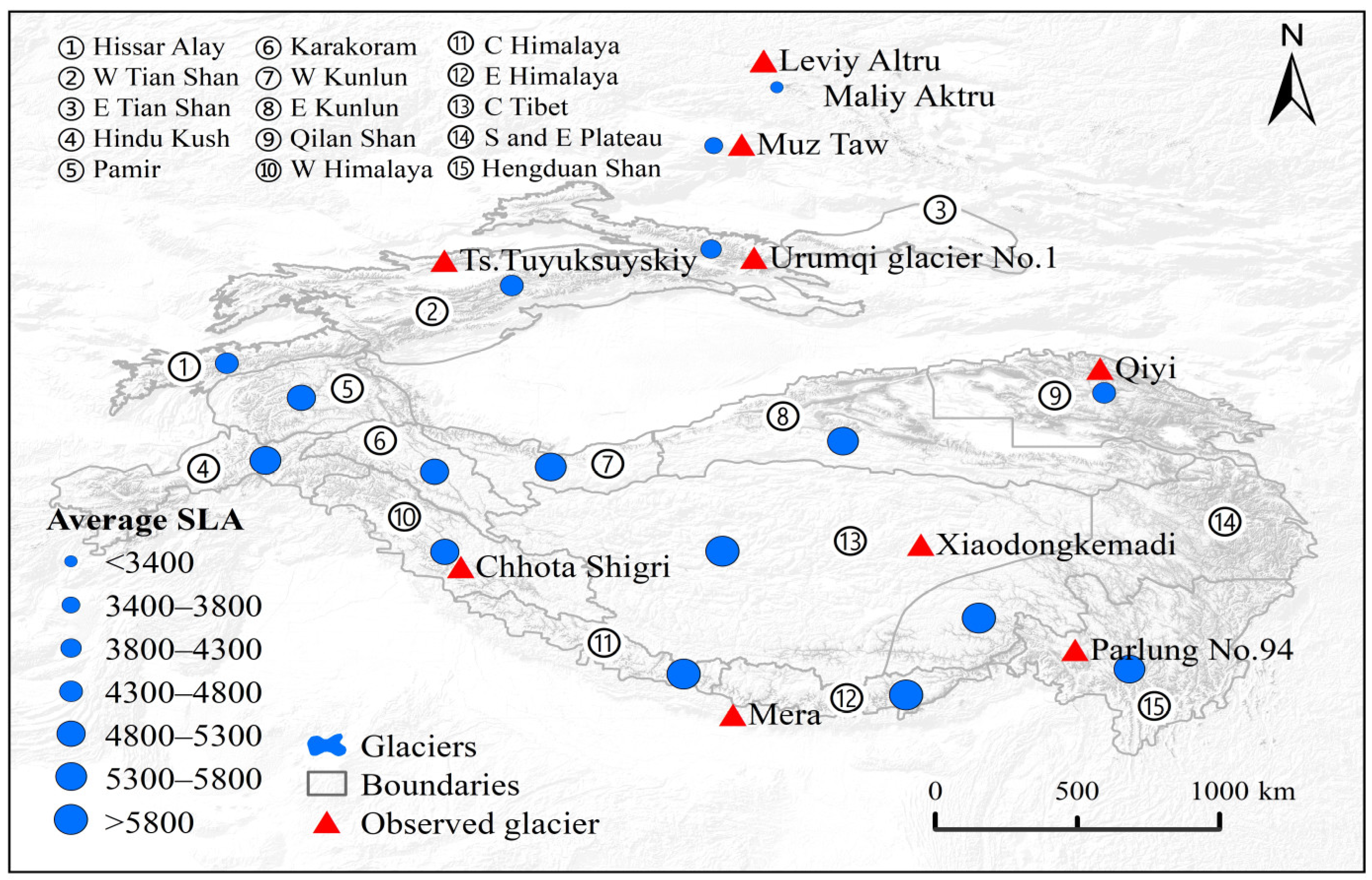
5.5. Comparison of SLA with Other Glaciers in High Mountain Asia
6. Conclusions
Author Contributions
Funding
Data Availability Statement
Conflicts of Interest
References
- Yao, T.; Bolch, T.; Chen, D.; Gao, J.; Immerzeel, W.; Piao, S.; Su, F.; Thompson, L.; Wada, Y.; Wang, L.; et al. The imbalance of the Asian water tower. J. Nat. Rev. Earth Environ. 2022, 3, 1–15. [Google Scholar] [CrossRef]
- Miles, E.; McCarthy, M.; Dehecq, A.; Kneib, M.; Fugger, S.; Pellicciotti, F. Health and sustainability of glaciers in High Mountain Asia. Nat. Commun. 2021, 12, 2868. [Google Scholar] [CrossRef] [PubMed]
- Wang, P.; Li, Z.; Li, H.; Cao, M.; Wang, W.; Wang, F. Glacier No.4 of Sigong River over Mt. Bogda of eastern Tianshan, central Asia: Thinning and retreat during the period 1962–2009. Environ. Earth Sci. 2012, 66, 265–273. [Google Scholar] [CrossRef]
- Zemp, M.; Huss, M.; Thibert, E.; Eckert, N.; McNabb, R.; Huber, J.; Barandun, M.; Machguth, H.; Nussbaumer, S.U.; Gärtner-Roer, I.; et al. Global glacier mass changes and their contributions to sea-level rise from 1961 to 2016. Nature 2019, 568, 382–386. [Google Scholar] [CrossRef] [PubMed]
- Wang, P.; Li, Z.; Huai, B.; Wang, W.; Li, H.; Wang, L. Spatial variability of glacier changes and their effects on water resources in the Chinese Tianshan Mountains during the last five decades. J. Arid. Land 2015, 7, 717–727. [Google Scholar] [CrossRef]
- Yao, T.; Wu, G.; Xu, B.; Wang, W.; Gao, J.; An, B. Asian Water Tower Change and its Impacts. Bull. Chin. Acad. Sci. 2019, 34, 1203–1209. [Google Scholar]
- Wang, P.; Li, Z.; Li, H.; Wang, W.; Zhou, P.; Wang, L. Characteristics of a partially debris-covered glacier and its response to atmospheric warming in Mt. Tomor, Tien Shan, China. J. Glob. Planet. Change 2017, 159, 11–24. [Google Scholar] [CrossRef]
- Qin, D.; Ding, Y.; Xiao, C.; Kang, S.; Ren, J.; Yang, J.; Zhang, S. Cryospheric science: Research framework and disciplinary system. J. Natl. Sci. Rev. 2018, 5, 255–268. [Google Scholar] [CrossRef]
- Bliss, A.; Hock, R.; Radić, V. Global response of glacier runoff to twenty-first century climate change. J. Geophys. Res. Earth Surf. 2014, 119, 717–730. [Google Scholar] [CrossRef]
- Huai, B.; Li, Z.; Wang, F.; Wang, W.; Wang, P.; Li, K. Glacier volume estimation from ice-thickness data, applied to the Muz Taw glacier, Sawir Mountains, China. J. Environ. Earth Sci. 2015, 74, 1861–1870. [Google Scholar]
- Wang, Y.; Zhao, J.; Li, Z.; Zhang, M. Glacier changes in the Sawuer Mountain during 1977-2017 and their response to climate change. J. Nat. Resour. 2019, 34, 802–814. [Google Scholar] [CrossRef]
- Brock, B.W. An analysis of short-term albedo variations at Haut Glacier d’Arolla, Switzerland. J. Geogr. Ann. Ser. A., Phys. Geogr. 2004, 86, 53–65. [Google Scholar] [CrossRef]
- Seo, M.; Kim, H.C.; Huh, M.; Yeom, J.M.; Lee, C.S.; Lee, K.S.; Choi, S.; Han, K.S. Long-Term variability of surface albedo and its correlation with climatic variables over Antarctica. Remote Sens. 2016, 8, 981. [Google Scholar] [CrossRef]
- Zhang, Y.; Gao, T.; Kang, S.; Shangguan, D.; Luo, X. Albedo reduction as an important driver for glacier melt in Tibetan Plateau and its surrounding areas. Earth Sci. Rev. 2021, 220, 103735. [Google Scholar] [CrossRef]
- Dickinson, R.E. Land surface processes and climate-surface albedos and energy balance. Adv. Geophys. 1983, 25, 305–353. [Google Scholar]
- Dumont, M.; Gardelle, J.; Sirguey, P.; Guillot, A.; Six, D.; Rabatel, A.; Arnaud, Y. Linking glacier annual mass balance and glacier albedo retrieved from MODIS data. Cryosphere 2012, 6, 1527–1539. [Google Scholar] [CrossRef]
- Wu, X.; Wang, N.; Lu, A.; Pu, J.; Guo, Z.; Zhang, H. Variations in albedo on Dongkemadi glacier in Tanggula Range on the Tibetan Plateau during 2002–2012 and its linkage with mass balance. Arct. Antarct. Alp. Res. 2015, 47, 281–292. [Google Scholar] [CrossRef]
- Cogley, J.G.; Hock, R.; Rasmussen, L.A.; Arendt, A.A.; Bauder, A.; Braithwaite, R.J.; Jansson, P.; Kaser, G.; MÖler, M.; Nicholson, L.; et al. Glossary of Glacier Mass Balance and Related Terms; IHP-VII Technical Documents in Hydrology, No. 86, IACS Contribution No. 2; UNESCO: Paris, France, 2011; p. 965. [Google Scholar]
- Kaur, R.; Saikumar, D.; Kulkarni, A.V.; Chaudhary, B.S. Variations in snow cover and snowline altitude in Baspa Basin. Curr. Sci. 2009, 96, 1255–1258. [Google Scholar]
- Cuffey, K.M.; Paterson, W.S.B. The Physics of Glaciers; Academic Press: Cambridge, MA, USA, 2010. [Google Scholar]
- Barandun, M.; Huss, M.; Usubaliev, R.; Azisov, E.; Berthier, E.; Kääb, A.; Bolch, T.; Hoelzle, M. Multi-decadal mass balance series of three Kyrgyz glaciers inferred from modelling constrained with repeated snow line observations. Cryosphere 2018, 12, 1899–1919. [Google Scholar] [CrossRef]
- Wang, J.; Ye, B.; Cui, Y.; He, X.; Yang, G. Spatial and temporal variations of albedo on nine glaciers in western China from 2000 to 2011. Hydrol. Process. 2014, 28, 3454–3465. [Google Scholar] [CrossRef]
- Yue, X.; Li, Z.; Li, H.; Wang, F.; Jin, S. Multi-Temporal Variations in Surface Albedo on Urumqi Glacier No.1 in Tien Shan, under Arid and Semi-Arid Environment. Remote Sens. 2022, 14, 808. [Google Scholar] [CrossRef]
- Tang, Z.; Wang, J.; Liang, J.; Li, C.; Wang, X. Monitoring of Snowline Altitude over the Tibetan Plateau Based on MODIS Data. Remote Sens. Technol. Appl. 2015, 30, 767–774. [Google Scholar]
- Hall, D.K.; Ormsby, J.P.; Bindschadler, R.A.; Siddalingaian, H. Characterization of snow and ice reflectance zones on glaciers using Landsat Thematic Mapper data. Ann. Glaciol. 1987, 9, 104–108. [Google Scholar] [CrossRef]
- De Angelis, H.; Rau, F.; Skvarca, P. Snow zonation on Hielo Patagónico Sur, Southern Patagonia, derived from Landsat 5 TM data. Glob. Planet. Change 2007, 59, 149–158. [Google Scholar] [CrossRef]
- Klein, A.G.; Isacks, B.L. Spectral mixture analysis of Landsat thematic mapper images applied to the detection of the transient snowline on tropical Andean glaciers. Glob. Planet. Change 1999, 22, 139–154. [Google Scholar] [CrossRef]
- Heiskanen, J.; Kajuutti, K.; Pellikka, P. Mapping glacier changes, snowline altitude and AAR using Landsat data in Svartisen, northern Norway. Geophys. Res. Abstr. 2003, 5, 10328. [Google Scholar]
- Rastner, P.; Prinz, R.; Notarnicola, C.; Nicholson, L.; Sailer, R.; Schwaizer, G.; Paul, F. On the Automated Mapping of Snow Cover on Glaciers and Calculation of Snow Line Altitudes from Multi-Temporal Landsat Data. Remote Sens. 2019, 11, 1410. [Google Scholar] [CrossRef]
- Guo, Z.; Wang, N.; Kehrwald, M.N.; Mao, R.; Wu, H.; Wu, Y.; Jiang, X. Temporal and spatial changes in Western Himalayan firn line altitudes from 1998 to 2009. Glob. Planet. Change 2014, 118, 97–105. [Google Scholar] [CrossRef]
- Yue, X.; Li, Z.; Zhao, J.; Li, H.; Wang, P.; Wang, L. Changes in the End-of-Summer Snow Line Altitude of Summer-Accumulation-Type Glaciers in the Eastern Tien Shan Mountains from 1994 to 2016. Remote Sens. 2021, 13, 1080. [Google Scholar] [CrossRef]
- Lanzhou Institute of Glaciology and Geocryology, Chinese Academy of Sciences. Glacier Inventory of China (II): Altay Mountains; Science Press: Beijing, China, 1982. [Google Scholar]
- Shi, Y.F. Concise China Glacier Inventory; Shanghai Popular Science Press: Shanghai, China, 2005; pp. 101–105. [Google Scholar]
- Wang, Z.T. New statistical figures and distribution feature of glaciers on the various Mountains in China. J. Glaciol Geocryol. 1988, 11, 8–14. [Google Scholar]
- Wang, F.; Yue, X.; Wang, L.; Li, H.; Du, Z.; Ming, J.; Li, Z. Applying artificial snowfall to reduce the melting of the Muz Taw Glacier, Sawir Mountains. Cryosphere 2020, 14, 2597–2606. [Google Scholar] [CrossRef]
- Panagiotopoulos, F.; Shahgedanova, M.; Hannachi, A.; Stephenson, D.B. Observed Trends and Teleconnections of the Siberian High: A Recently Declining Center of Action. J. Clim. 2005, 18, 1411–1422. [Google Scholar] [CrossRef]
- Klok, E.J.; Greuell, W.; Oerlemans, J. Temporal and spatial variation of the surface albedo of Morteratschgletscher, Switzerland, as derived from 12 Landsat images. J. Glaciol. 2003, 49, 491–502. [Google Scholar] [CrossRef]
- Adler-Golden, S.M.; Matthew, M.W.; Bernstein, L.S.; Levine, R.Y.; Berk, A.; Richtsmeier, S.C.; Acharya, P.K.; Anderson, G.P.; Felde, G.; Gardner, J.; et al. Atmospheric correction for shortwave spectral imagery based on MODTRAN4. Imaging Spectrom. V. 1999, 3735, 61–69. [Google Scholar]
- McDonald, E.R.; Wu, X.; Caccetta, P. Illumination Correction of Landsat TM data in South East NSW; Environment Australia: Canberra, Australia, 2002; pp. 8–25. [Google Scholar]
- Huang, W.; Zhang, L.; Li, P. An improved topographic correction approach for satellite image. J. Image Graph. 2005, 10, 1124–1129. [Google Scholar]
- Duguay, C.R.; Ledrew, E.F. Estimating surface reflectance and albedo over rugged terrain from Landsat-5 Thematic Mapper. Photogramm. Eng. Remote Sens. 1992, 58, 551–558. [Google Scholar]
- Hall, D.K.; Riggs, G.A. MODIS/Terra Snow Cover Daily L3 Global 500 m SIN Grid, [2000–2021], Version 61; NASA National Snow and Ice Data Center Distributed Active Archive Center: Boulder, CO, USA, 2021. [Google Scholar]
- Klein, A.G.; Stroeve, J. Development and validation of a snow albedo algorithm for the MODIS Instrument. Ann. Glaciol. 2002, 34, 45–52. [Google Scholar] [CrossRef]
- Liang, S.; Fang, H.; Chen, M.; Shuey, C.J.; Walthall, C.; Daughtry, C.; Morisette, J.; Schaaf, C.; Strahler, A. Validating MODIS land surface reflectance and albedo products: Methods and preliminary results. Remote Sens. Environ. 2002, 83, 149–162. [Google Scholar] [CrossRef]
- Gunnarsson, A.; Gardarsson, S.M.; Pálsson, F.; Jóhannesson, T.; Sveinsson, Ó.G.B. Annual and inter-annual variability and trends of albedo of Icelandic glaciers. Cryosphere 2021, 15, 547–570. [Google Scholar] [CrossRef]
- Zhu, M.; Yao, T.; Yang, W.; Maussion, F.; Huintjes, E.; Li, S. Energy-and mass-balance comparison between Zhadang and Parlung No. 4 glaciers on the Tibetan Plateau. J. Glaciol. 2015, 61, 595–607. [Google Scholar] [CrossRef]
- Dowson, A.J.; Sirguey, P.; Cullen, N.J. Variability in glacier albedo and links to annual mass balance for the gardens of Eden and Allah, Southern Alps, New Zealand. Cryosphere 2020, 14, 3425–3448. [Google Scholar] [CrossRef]
- Thind, P.S.; Chandel, K.K.; Sharma, S.K.; Mandal, T.K.; John, S. Light-absorbing impurities in snow of the Indian Western Himalayas: Impact on snow albedo, radiative forcing and enhanced melting. Environ. Sci. Pollut. Res. 2019, 26, 7566–7578. [Google Scholar] [CrossRef] [PubMed]
- Wang, P.; Li, Z.; Li, H.; Wang, W.; Yao, H. Comparison of glaciological and geodetic mass balance at Urumqi Glacier No. 1, Tian Shan, Central Asia. Glob. Planet. Change 2014, 114, 14–22. [Google Scholar] [CrossRef]
- Liu, Y.; Qin, X.; Chen, J.; Li, Z.; Wang, J.; Du, W.; Guo, W. Variations of Laohugou Glacier No. 12 in the western Qilian Mountains, China, from 1957 to 2015. J. Mt. Sci. 2018, 15, 25–32. [Google Scholar] [CrossRef]
- Yao, T.; Thompson, L.; Yang, W.; Gao, Y.; Guo, X.; Yang, X.; Duan, K.; Zhao, H.; Xu, B.; Pu, J.; et al. Different glacier status with atmospheric circulations in Tibetan Plateau and surroundings. Nat. Clim. Change 2012, 2, 663–667. [Google Scholar] [CrossRef]
- Wang, X.; Tang, Z.; Wang, J.; Wang, X.; Wei, J. Monitoring of snowline altitude at the end of melt season in High Mountain Asia based on MODIS snow cover products. Acta Geogr. Sin. 2020, 75, 470–484. [Google Scholar]
- Ye, W.; Wang, F.; Li, Z.; Zhang, H.; Xu, C.; Huai, B. Temporal and spatial distributions of the equilibrium line altitudes of the monitoring glaciers in High Asia. J. Glaciol. Geocryol. 2016, 38, 1459–1469. [Google Scholar]
- Guo, Z.; Wang, N.; Shen, B.; Gu, Z.; Wu, Y.; Chen, A. Recent Spatiotemporal Trends in Glacier Snowline Altitude at the End of the Melt Season in the Qilian Mountains, China. Remote Sens. 2021, 13, 4935. [Google Scholar] [CrossRef]
- Guo, Z.; Geng, L.; Shen, B.; Wu, Y.; Chen, A.; Wang, N. Spatiotemporal Variability in the Glacier Snowline Altitude across High Mountain Asia and Potential Driving Factors. Remote Sens. 2021, 13, 425. [Google Scholar] [CrossRef]
- Yang, W.; Guo, X.; Yao, T.; Zhu, M.; Wang, Y. Recent accelerating mass loss of southeast Tibetan glaciers and the relationship with changes in macroscale atmospheric circulations. Clim. Dyn. 2016, 47, 805–815. [Google Scholar] [CrossRef]


| Path/Row | Date | Sensor | Cloud Cover |
|---|---|---|---|
| 145/27 | 12 July 2011 | Landsat ETM+ | 1% |
| 16 September 2012 | Landsat ETM+ | 5% | |
| 3 September 2013 | Landsat ETM+ | 0 | |
| 29 August 2014 | Landsat OLI | 0.13% | |
| 15 July 2015 | Landsat OLI | 0.02% | |
| 26 August 2016 | Landsat ETM+ | 0 | |
| 5 June 2018 | Landsat OLI | 1.2% | |
| 7 July 2018 | Landsat OLI | 0.93% | |
| 27 August 2019 | Landsat OLI | 0.02% | |
| 14 October 2019 | Landsat OLI | 0.25% | |
| 9 May 2020 | Landsat OLI | 0.54% | |
| 14 September 2020 | Landsat OLI | 1.9% | |
| 24 August 2021 | Landsat ETM+ | 0 |
Publisher’s Note: MDPI stays neutral with regard to jurisdictional claims in published maps and institutional affiliations. |
© 2022 by the authors. Licensee MDPI, Basel, Switzerland. This article is an open access article distributed under the terms and conditions of the Creative Commons Attribution (CC BY) license (https://creativecommons.org/licenses/by/4.0/).
Share and Cite
Yu, F.; Wang, P.; Li, H. Surface Albedo and Snowline Altitude Estimation Using Optical Satellite Imagery and In Situ Measurements in Muz Taw Glacier, Sawir Mountains. Remote Sens. 2022, 14, 6405. https://doi.org/10.3390/rs14246405
Yu F, Wang P, Li H. Surface Albedo and Snowline Altitude Estimation Using Optical Satellite Imagery and In Situ Measurements in Muz Taw Glacier, Sawir Mountains. Remote Sensing. 2022; 14(24):6405. https://doi.org/10.3390/rs14246405
Chicago/Turabian StyleYu, Fengchen, Puyu Wang, and Hongliang Li. 2022. "Surface Albedo and Snowline Altitude Estimation Using Optical Satellite Imagery and In Situ Measurements in Muz Taw Glacier, Sawir Mountains" Remote Sensing 14, no. 24: 6405. https://doi.org/10.3390/rs14246405
APA StyleYu, F., Wang, P., & Li, H. (2022). Surface Albedo and Snowline Altitude Estimation Using Optical Satellite Imagery and In Situ Measurements in Muz Taw Glacier, Sawir Mountains. Remote Sensing, 14(24), 6405. https://doi.org/10.3390/rs14246405