Article

Regional Satellite Algorithms to Estimate Chlorophyll-a and Total Suspended Matter Concentrations in Vembanad Lake

1
Plymouth Marine Laboratory, Plymouth PL1 3DH, UK
2
National Centre for Earth Observation, Plymouth Marine Laboratory, Plymouth PL1 3DH, UK
3
Nansen Environmental Research Centre, Amenity Centre, Kerala University of Fisheries and Ocean Sciences, Cochin 682506, Kerala, India
4
Indian Council of Agricultural Research-Central Marine Fisheries Research Institute, Cochin 682018, Kerala, India
5
Council of Scientific and Industrial Research-National Institute of Oceanography, Regional Centre, Cochin 682015, Kerala, India
6
Centre for Geography and Environmental Science, Faculty of Environment, Science and Economy, University of Exeter, Penryn TR10 9FE, UK
7
Faculty of Marine Sciences, Cochin University of Science and Technology, Cochin 682022, Kerala, India
*
Author to whom correspondence should be addressed.
Remote Sens. 2022, 14(24), 6404; https://doi.org/10.3390/rs14246404
Submission received: 14 November 2022 / Revised: 10 December 2022 / Accepted: 10 December 2022 / Published: 19 December 2022
(This article belongs to the Section Ocean Remote Sensing)

Abstract

:
A growing coastal population is leading to increased anthropogenic pollution that greatly affects coastal and inland water bodies, especially in the tropics. The Sustainable Development Goal-14, ‘Life below water’ emphasises the importance of conservation and sustainable use of the ocean and its resources. Pollution management practices often include monitoring of water quality using in situ observations of chlorophyll-a (chl-a) and total suspended matter (TSM). Satellite technology, including the MultiSpectral Instrument (MSI) sensor onboard Sentinel-2, enables the continuous monitoring of these variables in inland waters at high spatial and temporal resolutions. To improve the monitoring of water quality in the tropical Vembanad-Kol-Wetland (VKW) system, situated on the southwest coast of India, we present two regionally tuned satellite algorithms developed to estimate chl-a and TSM concentrations. The new algorithms estimate the chl-a and TSM concentrations from the simulated reflectance values as a function of the inherent optical properties using a forward modelling approach. The model was parameterised using the National Aeronautics and Space Administration (NASA) bio-Optical Marine Algorithm Dataset (NOMAD) and in situ measurements collected in the VKW system. To assess model performance, results were compared with in situ measurements of chl-a and TSM and other existing satellite-based models of chl-a and TSM. For satellite application, two different atmospheric correction methods (ACOLITE and POLYMER) were tested and satellite matchups were used to validate the new chl-a and TSM algorithms following standard validation procedures. The results demonstrated that the new algorithms were in good agreement with in situ observations and outperform existing chl-a and TSM algorithms. The new regional satellite algorithms can be used to monitor water quality within the VKW system to support the sustainable management under natural (cyclones, floods, rainfall, and tsunami) and anthropogenic pressures (industrial effluents, agricultural practices, recreational activities, construction, and demolishing concrete structures) and help achieve Sustainable Development Goal 14.

Graphical Abstract

1. Introduction

Coastal, estuarine, and inland waters are major carbon reservoirs [1,2,3,4]; support diverse species in multiple habitats; provide a wide range of ecosystem services; and function as natural barriers for the protection of coastal areas from extreme climate events, including floods, cyclones, and tsunamis [5]. However, anthropogenic activities, such as the overexploitation of resources and pollution, have adversely affected many coastal aquatic ecosystems and the livelihood of people living in the surrounding areas [6,7,8,9,10]. The United Nations, through its Sustainable Development Goals-6 and 14, emphasise the importance of clean water and sanitation, and the sustainable use of aquatic resources [11]. In this context, monitoring water quality becomes an important step in our efforts to understand the stresses on coastal and estuarine ecosystems that are associated with anthropogenic activities, and to move towards sustainable management of their resources [12,13,14]. Some of the most vulnerable of coastal and estuarine ecosystems are in the tropics [15,16,17,18,19], which merit particular attention.
In this paper, we study the water quality of a tropical coastal, estuarine and lake system, the Vembanad-Kol-Wetland (VKW) system, situated on the southwest coast of India. VKW is a large ecosystem, adjoining some of the major towns of the state Kerala, including Alappuzha, Kochi, Kottayam, and Thrissur. The population surrounding the VKW system relies on the waterbody for many aspects of their life: provision of drinking water, fishing, agriculture, transport, tourism, and aquaculture [20]. The shipyard and port at Kochi benefit from the waterways of VKW. Despite the importance of the VKW system, heavy loads of suspended particulate and dissolved matter and nutrients (which determine the concentration of chlorophyll-a, the major pigment in phytoplankton), and the prevalence of pathogenic organisms responsible for water-borne diseases have degraded the water quality of the system [21,22,23,24]. The VKW is one of the most polluted wetland systems in India, exposed to anthropogenic stresses that include the inflow of domestic waste and sewage causing faecal contamination, and heavy metal contamination from nearby industries [25,26,27,28,29]. Construction activities along its shorelines in violation of the Indian coastal zone management regulations present yet another threat to the integrity of the VKW ecosystem [30,31]. The ecological and economic importance of the VKW system, and the multiple stresses it is currently facing, raise the need for regular monitoring of its water quality, to enable recovery and restoration, and to achieve the sustainable development goals. In situ observations of water quality are essential in this context, but they are labour-intensive. Furthermore, the complex nature of the wetland system (about 100 km long, with many inlets and meanders) makes it costly to cover the entire lake by local observations alone. Citizen science can help address some of these limitations [31,32]. However, another important avenue that we explore here is the use of satellite data as a complement to in situ observations, for monitoring water quality on a sustained and continuous basis.
Chlorophyll-a (chl-a) and total suspended matter (TSM) are two major water constituents that affect water quality, and which are amenable to remote sensing. Many models have been developed to estimate chl-a and TSM concentrations from satellite observations. Among them, the model by O’Reilly et al. [33], which produces accurate results in the open-ocean waters, has been widely employed to estimate chl-a concentrations. To estimate high concentrations of chl-a (>100 mg m−3), especially in turbid, productive, and inland waters, models based on the ratio of near-infrared (NIR) reflectances [34,35,36,37] have been found to be more suitable. For the estimation of TSM, models based on reflectance at red and infrared wavelengths [38,39] have performed well in sediment-dominated waters. The VKW is an optically complex system with diverse types of water appearing in different areas of the system [25]. Therefore, we cannot assume that the above-mentioned algorithms would perform equally well throughout the system.
In this paper, we evaluate the performance of existing chl-a and TSM satellite retrieval algorithms, and use a forward modelling technique to develop improved algorithms in the study area. Though earlier studies have used satellite data to investigate the dynamics of chl-a and TSM in Vembanad lake using existing algorithms [40,41,42], to our knowledge, this is the first time that such algorithms have been validated using in situ-satellite matchup data. Furthermore, satellite-derived water-leaving reflectance ( ρ w ) values retrieved using two atmospheric-correction algorithms are fine-tuned using in situ observations. Using Sentinel-2 MultiSpectral Instrument (MSI) data, we demonstrate that the performance of the modified chl-a and TSM algorithms is better than those of existing algorithms for the VKW system.

2. Materials and Methods
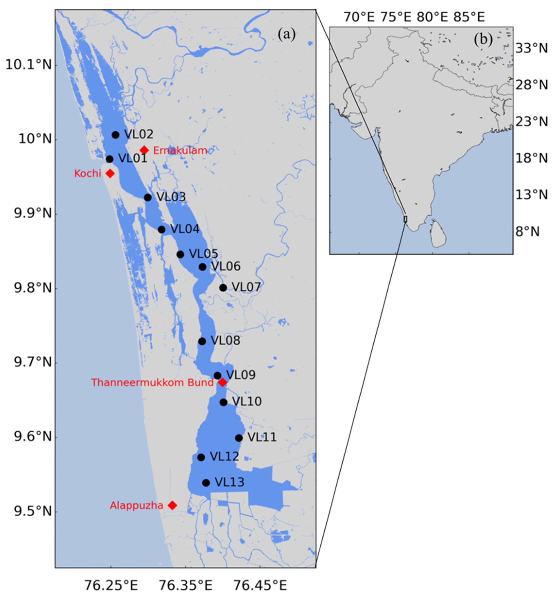
This study estimates reflectance as a function of the absorption and backscattering coefficients based on the in situ observations from Vembanad Lake and the NOMAD dataset, where the estimated reflectance was used to develop regionally tuned chlorophyll-a ( B ) and total suspended matter ( S ) algorithms suitable for Vemabanad Lake (Figure 1, discussed in detail in the following sections). The developed algorithms were applied on the MSI data after the atmospheric signal was removed based on the two different atmospheric correction methods, ACOLITE and POLYMER, and corrected using the satellite matchups to of estimated reflectance.

2.1. Study Site

Vembanad Lake (VL) is a part of the Vemband–Kol–Wetland (VKW) system, which is the second largest Ramsar site in India. The lake is ~100 km long and up to ~14 km wide and is open to the Arabian Sea in the north, near Kochi (Figure 2). Its depth varies from 1.5 to 6 m except near the port of Kochi, where a depth of 13 m is maintained by dredging to make it suitable for shipping [25]. The lake receives freshwater input from six major rivers [20]. The region experiences two monsoons: the south-west monsoon (June–September) and the north-east monsoon (October–November), which form the wet season. The dry season is during the winter (December–February) and the spring inter-monsoon (March–May) [43].
Based on salinity and hydrological conditions, VL can be divided into a brackish-water-dominated northern region (Stations VL01 to VL06, Figure 2) and a fresh-water-dominated southern region (Stations VL08 to VL13, Figure 2) [22]. The northern region also becomes dominated by freshwater during the monsoons. The Thanneermukkom Bund isolates the southern region (stations–VL10, VL11, VL12, and VL13) of the lake from the incursion of saltwater from the sea during the dry season.

2.2. In Situ Data from Vembanad Lake

In situ data, used for the development of regional satellite-algorithms (VL dataset, Table 1), were collected in VL at 13 stations (VL01–VL13, Figure 2) during 15 field campaigns between March 2018 and May 2019. Samples were collected for the analysis of bio-optical properties, including the absorption coefficients ( a ), the concentrations of chlorophyll-a biomass ( B ), and total suspended matter ( S ). Samples were filtered through 25 mm Whatman glass-fibre filters (GF/F) with a 0.7 μm pore size to collect the algal and non-algal particulate matter to determine the optical density ( D ) of phytoplankton biomass ( D B ), non-algal suspended particles ( D S ) and coloured dissolved organic matter (CDOM), or yellow substances ( D Y ). The filters were analysed using a Shimadzu Ultraviolet-Visible (UV) Spectrophotometer (UV-2600) following standard methods [44,45,46]. The filter, with all material retained on it, was used to determine the optical density of particulate matter (phytoplankton biomass + non-algal suspended particles) ( D B + S ). Phytoplankton pigments were removed from the filter using a methanol extraction, and the optical density D S of the residual material was measured. Then, D B was calculated by subtracting D S from D B + S [45,46]. For measuring D Y , water samples were filtered through 0.45 and 0.2 μm nitrocellulose filters [44,46], and the optical density of the filtrate was measured [47]. The D B , D S and D Y values were used to estimate their respective absorption coefficients ( a B ,   a S , and a Y ) [48,49,50].
To estimate the chlorophyll-a biomass ( B ), samples were filtered through 47 mm, 0.7 μm Whatman GF/F filters and phytoplankton pigments were extracted in 90% acetone for 24 h, and the optical density D B of the extract was measured spectrophotometrically at 630, 647, and 664 nm [51,52]. Then, the chlorophyll-a biomass was calculated using the equation, B = 11.85 × D B 664 1.54 × D B 647 0.08 × D B 630 × v / V × 1000 , where v is the volume of acetone (units in ml) and V is the volume of water (units in ml) filtered. Concentrations of total suspended matter ( S ) were measured gravimetrically by filtering the sample through pre-weighed 25 mm, 0.7 μm Whatman GF/F filters, which were then dried before weighing following standard techniques [53,54]. Table A1 provides details on the notations used in this study.

2.3. In Situ Data from NOMAD

In addition to the in situ measurements from VL, samples from the NASA bio-Optical Marine Algorithm Dataset (NOMAD) v2.0 (NOMAD dataset, Table 1) [55] were also used in this study for model parameterizations. NOMAD is a high-quality in situ dataset covering global waters and is used for developing ocean-colour models. For this study, the water-leaving radiance ( L w ), downwelling surface irradiance ( E s ), back-scattering coefficient ( b b ), absorption coefficient of particulate matter (phytoplankton biomass + non-algal suspended particles, a B + a S ); non-algal suspended particles ( a S ); coloured dissolved organic matter ( a Y ), and chlorophyll-a biomass ( B ) were extracted from this dataset. The remote-sensing reflectance ( R r s ) was calculated as the ratio of L w to E s and converted into irradiance reflectance ( R i ) using R i = Q × R r s , where Q is set to 3.14.

2.4. Satellite Dataset

Data acquired by the MultiSpectral Instrument (MSI) onboard Sentinel-2A and -2B between 2018–2019 were downloaded from the Copernicus Open Access Hub (https://scihub.copernicus.eu, accessed on 6 January 2021). The two tiles of Sentinel-2 that cover Vembanad Lake were downloaded, processed, and mosaiced to generate images of the entire study area. Two processors, ACOLITE and POLYMER, were used to correct for the atmospheric effects. ACOLITE (v20190326.0; [56,57]) is based on the ‘dark spectrum fitting’ approach and POLYMER developed by Steinmetz et al. [58] removes the atmospheric signal and estimates the water-leaving reflectance using a polynomial function of the wavelength. The water-leaving reflectances ( ρ w ), derived from ACOLITE and POLYMER, were used to retrieve B and S . For simplicity, hereafter, the water-leaving reflectance ( ρ w ) from satellites will be referred to as ‘satellite reflectance’.

2.5. In Situ Satellite Matchup Dataset

In situ data from VL was matched with the corresponding Sentinel-2 data to construct a dataset, called the Satellite matchup dataset (Table 1), which was used for the validation of regional satellite-retrieval algorithms of B and S . Comparison between the modelled ( R e ) (described in the later Section 2.6 and Section 2.7) and satellite ( ρ w ) reflectance demonstrated some systematic biases. Therefore, a correction is calculated as: ρ w = l + ρ w × m , where l and m are fitted coefficients (Figure A1) that were applied to the processed satellite data. For both ACOLITE- and POLYMER-processed data, the intercept l was wavelength independent and equal to 0.0 and 0.01, respectively. For the five MSI wavebands—443, 490, 560, 665, and 705 nm—the values of the slope m were, respectively, 1.6, 2.0, 2.2, 1.6, and 1.2 for ACOLITE, and 3.5, 3.6, 3.8, 3.7, and 3.6 for POLYMER. The MSI products for the VL waters demonstrated that reflectances at bands 665 and 705 nm were frequently negative for POLYMER data before the bias correction, but were pushed to positive values with the addition of the offset. ACOLITE did not have the problem of negative values occurring at the long wavebands. Due to the small number of satellite matchups, all of them ( N = 12 and 14 for ACOLITE, and POLYMER, respectively) were used to correct satellite reflectances.
Standard quality control methods were followed for the in situ satellite matchup [59]: (i) the covariance of the 3 × 3 pixel box (central pixel plus surrounding eight pixels) was less than 0.15 for the five Sentinel-2 reflectance bands, to ensure the homogeneity of the pixel box; (ii) more than fifty percent of the pixel box must contain valid data (i.e., was not ‘Not A Number’ or negative); (iii) the time difference between the in situ and satellite overpass was within ± 4 h. For the matchup data that passed the quality criteria, the mean value of reflectances at each MSI waveband of the pixel box were computed and used as the input to the B and S algorithms. Based on these criteria, 12 and 14 satellite matchups were available for the ACOLITE- and POLYMER-processed satellite data, respectively.

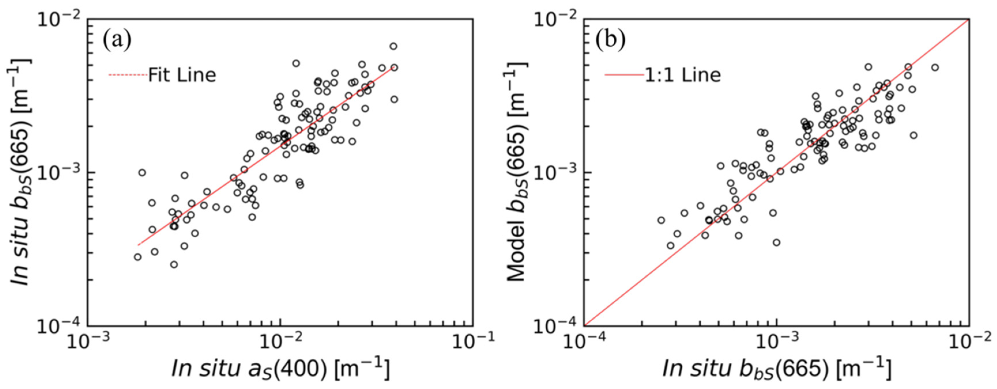
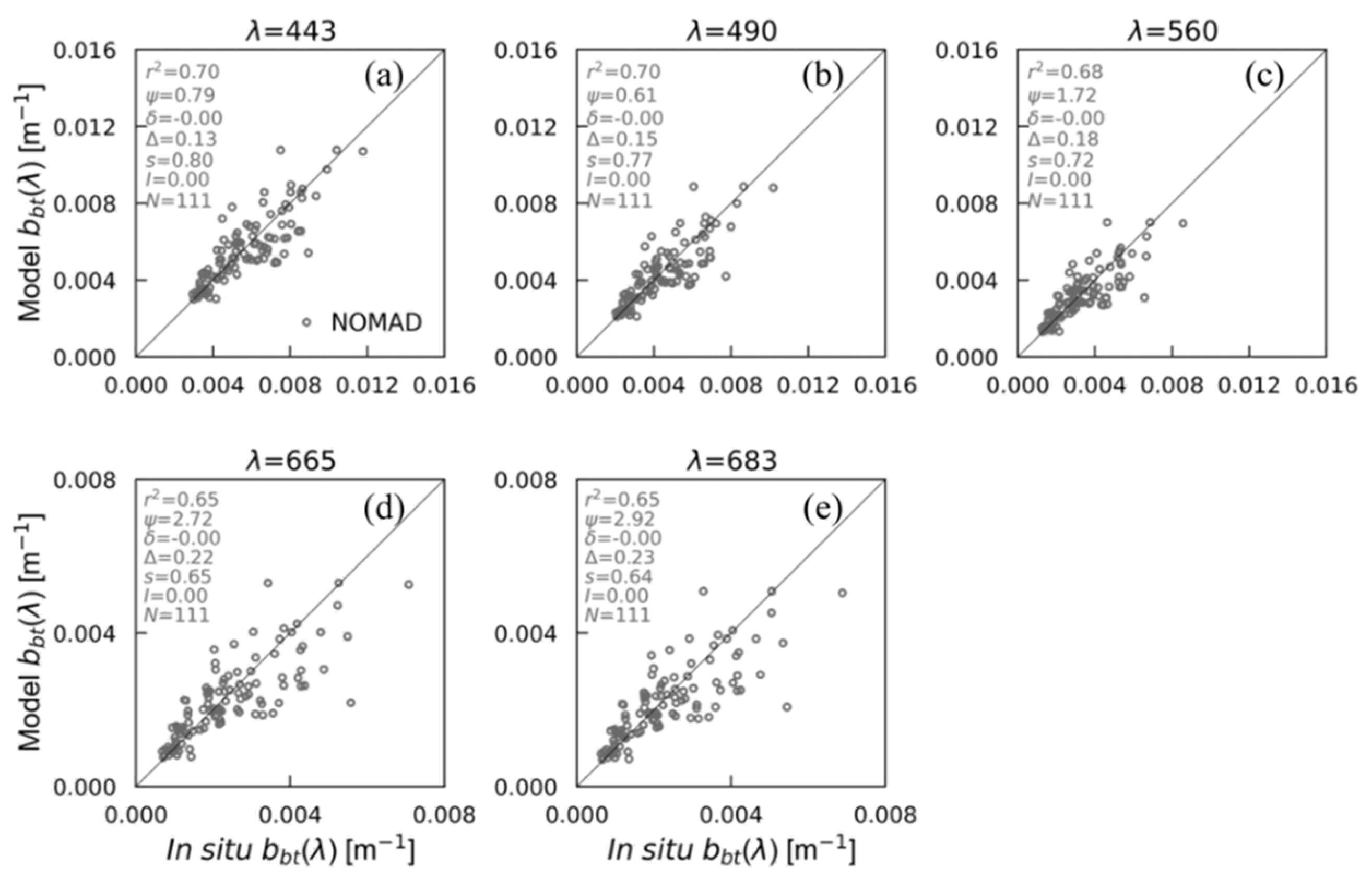
2.6. Inherent Optical Properties
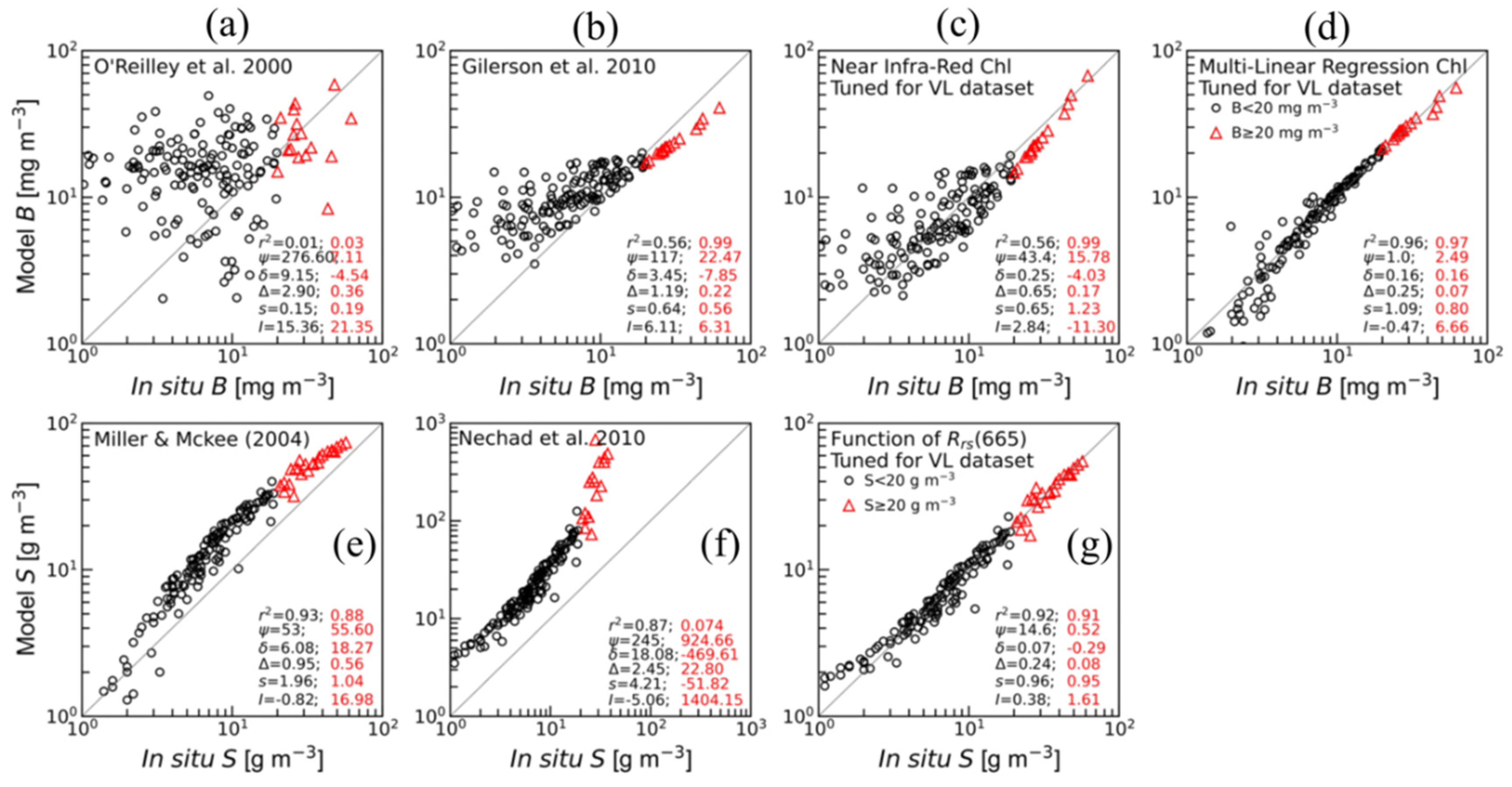
This section presents models to estimate the inherent optical properties (IOPs), and the absorption ( a ) and back-scattering ( b b ) coefficients, of the constituents present in the water column. The absorption is contributed by water ( a W ), phytoplankton as indexed by chlorophyll-a biomass ( a B ), non-algal suspended particles ( a S ), and CDOM ( a Y ). Thus, the total absorption coefficient ( a t ) can be expressed as:
a t λ = a W λ + a B λ + a S λ + a Y λ
where the individual contribution of each constituent to a t is represented by the subscripts W , B , S , and Y . The a W values were taken from Pope and Fry [60].
In this study, the method of Brewin et al. [61,62] was used to estimate a B λ values with the chlorophyll-a concentration as the input to the computation. In this approach, a B is the sum of the absorptions of three different size classes of phytoplankton, namely picophytoplankton ( a p in m−1), nanophytoplankton ( a n in m−1), and micro-phytoplankton ( a m in m−1):
a B λ = a p λ + a n λ + a m λ
Furthermore, each of the components of a B can be expressed as the product of the specific absorption coefficient of each phytoplankton size class and its respective biomass (in chlorophyll-a units), such that Equation (2) can be rewritten as:
a B λ = a p * λ × B p + a n * λ × B n + a m * λ × B m
where a p * ,   a n * , and a m * are the chlorophyll-specific absorption coefficients (in m2 (mg chl-a)−1) and B p , B n , and B m are the specific concentrations (in mg chl-a m−3) of the pico-, nano-, and micro-phytoplankton size classes, respectively. The specific absorption coefficients of each size class can be found in Table 2 of Brewin et al. [61]. The concentration of each size class was estimated using the following set of equations, which are all functions of the total chlorophyll-a biomass concentration, B:
B p = B p m 1 exp S p B
B p , n = B p , n m 1 exp S p , n B
B n = B p , n B p
B m = B B p , n
where the asymptotic maximum values B p m and B p , n m are 0.13, and 0.77, respectively, and the slopes S p and S p , n are 6.15, and 1.22, respectively [62]. Note that B n was estimated by subtracting Bp from the combined concentration of pico- and nano-phytoplankton ( B p , n ) biomass, as shown in Equation (5).
The spectral form of a S and a Y can be described by exponential functions with negative slopes, as their absorptions decrease with increasing wavelength:
a S λ = a S 400 × exp m S × λ 400
a Y λ = a Y 412 × exp m Y × λ 412
where a S 400 and a Y 412 are the absorption coefficient of the non-algal suspended particles at 400 nm and the CDOM absorption coefficient at 412 nm; and m S and m Y are the spectral slopes of a S and a Y , for which we assumed values of 0.012 [63] and 0.015 [64,65], respectively. The values of a t can be computed once a B , a S and a Y are estimated from the Equations (2), (8) and (9) in Equation (1), respectively.
When it came to modelling particle back-scattering, we faced a conundrum: neither the NOMAD nor the VL datasets included all the elements necessary for parameterising particle back-scattering as a function of total suspended matter. The VL dataset included measurements of total suspended matter ( S ) concentration and absorption coefficient of non-algal suspended particle ( a S ), but not non-algal suspended particle back-scattering ( b b S ). On the other hand, the NOMAD dataset included non-algal suspended particle back-scattering ( b b S ) and absorption coefficient of non-algal suspended particle ( a S ), but not the total suspended matter ( S ) concentration. The path we followed, therefore, was to use the common measurement of the non-algal suspended particle absorption coefficient ( a S ) to link back-scattering by non-algal suspended particles ( b b S ) and the concentration of total suspended matter ( S ), as described below.
First, the back-scattering coefficient of non-algal particles at 665 nm b b S 665 was expressed as a function of a s 400 , using the NOMAD dataset ( N = 91 , Figure 3a) as:
b b S 665 = 0.083 a S 400 0.873
Then, the modelled b b S 665 was used to estimate S using the relationship between b b S 665 and S proposed by Balasubramanian et al. [66] (Figure A2), based on data from a variety of locations and environmental conditions:
S = 53.736 × b b S 665 0.856
Next, the total back-scattering coefficient ( b b t ) in the NOMAD dataset was treated as the sum of the contributions to back-scattering by water ( b b W ) and non-algal suspended particle ( b b S ), and the contribution of phytoplankton is assumed to be relatively small compared with that of non-algal suspended particles for our study area where the non-algal suspended particle scattering dominates that of phytoplankton, such that we have:
b b t λ = b b W λ + b b S λ
The spectral values of b b W were taken from Morel [67]. The spectral variation in b b S derived from the equation above was then represented as [68]:
b b S λ = b b S 665 × λ 665 k
where the exponent k determines the spectral variations in b b S , which was estimated as 1.32 by fitting Equation (13) to b b S λ . For the NOMAD dataset, b b S 665 was computed using Equation (10), and tested against in situ data (Figure 3b). Due to the lack of in situ b b from VL, the b b model was only compared with the NOMAD dataset. For the Vembanad Lake dataset, we estimated the back-scattering coefficient of non-algal suspended particle ( b b S 665 ) at 665 nm from measured S, by inverting Equation (11):
b b S ( 665 ) = ( S 53.736 ) ( 1 0.856 )
The computed b b S values were then used in Equation (12) to estimate b b t .
Table 2. Table showing the different satellite-retrieval algorithms and their coefficients used in the present work to estimate chlorophyll-a ( B ) and total suspended matter ( S ) concentrations.
AlgorithmsEquationsVariablesReferences
B1 B = 10 0.19 1.81 X + 1.97 X 2 2.56 X 3 0.722 X = l o g 10 R r s 443 / R r s 560 O’Reilly et al. [33] with parameters from Franz et al. [69] and Vanhellemont and Ruddick [70]
B2 B = 35.8 X 19.3 1.12 X = R r s 705 / R r s 665 Gilerson et al. [36]
B3 B = 40.6 138 X + 122 X 2 X = R r s 705 / R r s 665 This study
B4 B = 55.0 56.1 X 1 + 50.3 X 2 20.8 X 3 + 89.0 X 4 X 1 = R r s 443 / R r s 560   X 2 = R r s 490 / R r s 560   X 3 = R r s 665 / R r s 560   X 4 = R r s 705 / R r s 665 This study
S1 S = 1.91 + 1140 X X = R r s 665 Miller and McKee [38]
S2 S = 1.74 + 356 X 1 X / 0.1728 X = R 665 Nechad et al. [39]
S3 S = 1.1 + 332 X + 7188 X 2 X = R r s 665 This study

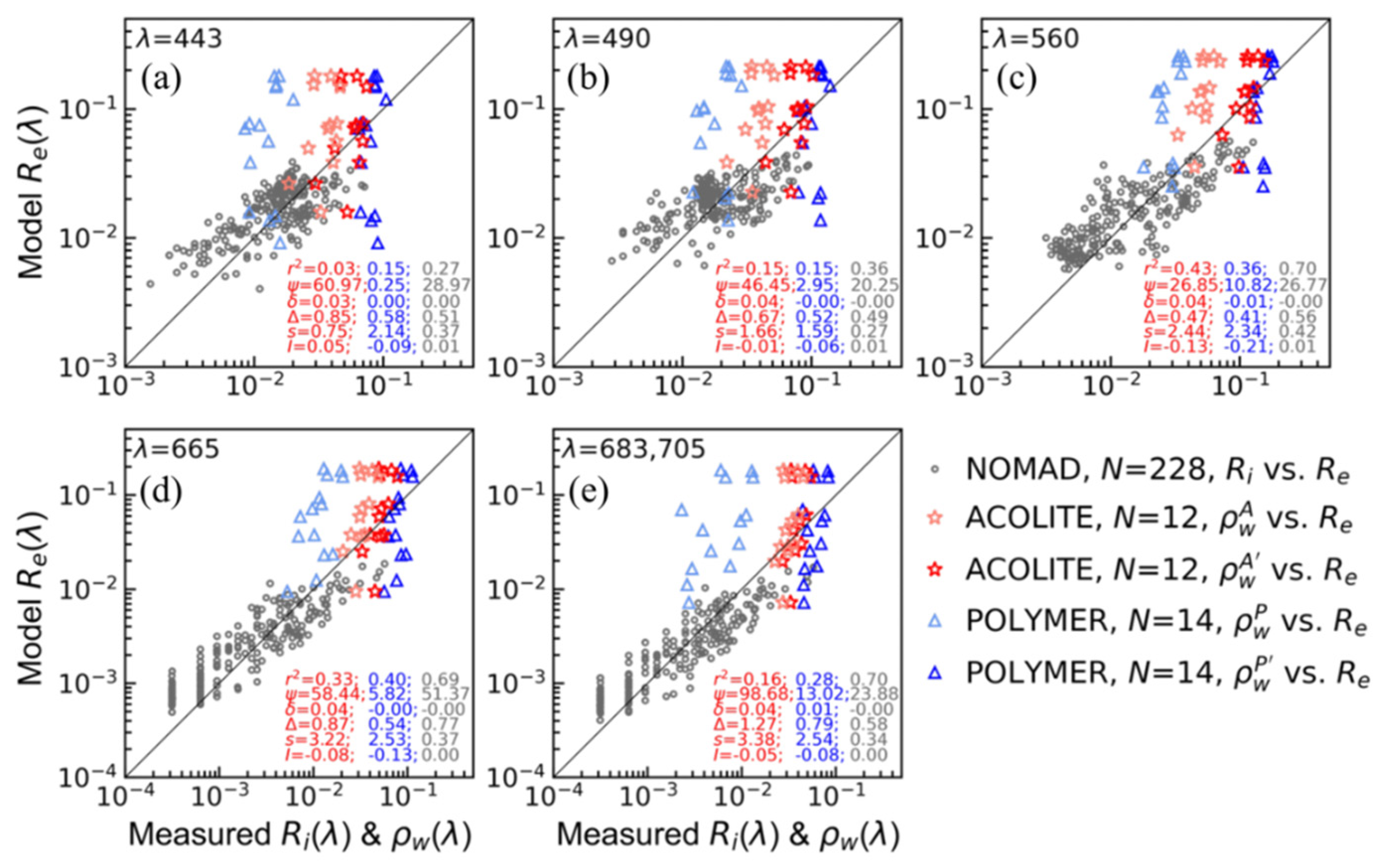
2.7. Forward Reflectance Model

The IOPs were used to model reflectance R e (Morel and Prieur [71]; see also Sathyendranath and Platt [72]) as:
R e λ = 0.33 × b b t λ a t λ + b b t λ .

2.8. Chl-a and TSM Satellite Algorithms

The computed R e values were used to develop regional satellite algorithms for retrieval of B and S in VL. Several existing and newly-developed algorithms (Table 2) were tested to evaluate the efficiency of B and S retrieval in VL using the VL dataset ( N = 162 , Table 1).
To estimate B , the algorithms of O’Reilly et al. [33], based on a blue-green reflectance ratio (Algorithm B1; Table 2) and Gilerson et al. [36], based on a NIR reflectance band ratio (Algorithm B2; Table 2) were examined, as they are both used extensively in the literature for open-ocean waters [33], and for more complex coastal waters [36]. The model coefficients used by Gilerson et al. [36] were tuned to improve the performance of this algorithm (Algorithm B3; Table 2) using the VL dataset. In addition, by experimenting with different combinations of reflectance bands, a new algorithm based on multi-linear regression (BGR, Algorithm B4, Table 2) was introduced that used all five reflectance bands from Sentinel-2.
For the estimation of S in VL, the algorithms of Miller and McKee [38] (Algorithm S1, Table 2) and Nechad et al. [39] (Algorithm S2, Table 2) were tested. It has been reported that reflectance in the red bands increases with S , especially in sediment-dominated turbid waters [73]. In VL, a polynomial relationship was observed (Algorithm S3, Table 2) between R e 665 and in situ S :
S exp R e 665
and this relationship was also explored, to estimate S from satellite data.
The performance of all B and S algorithms (Table 2) were assessed based on the following statistical metrics: determination coefficient ( r 2 ), root mean square error ( ψ ), bias ( δ ), mean relative error ( ), and the slope ( s ), and the intercept ( I ) of a linear fit between the model and observations.

3. Results

3.1. Inherent Optical Properties

The comparison between the in situ and model-derived values of a B , a S , a Y , and a t at the five key wavelengths demonstrated that the modelled absorption values were consistent with in situ measurements, both from the VL ( N = 228 ) and NOMAD ( N = 839 ) datasets (Figure 4). The model-derived a Y showed more scatter at 665 and 683 nm compared with the a B and a S estimates at the same wavelengths (Figure 4i,j), but the effect on the total absorption values ( a t ) is insignificant, as the magnitude of a Y is small compared with the absorption coefficients of the other constituents ( a W , a B , and a S ) at these wavelengths (Figure 4s,t). The estimated b b t values are in close agreement with in situ values from the NOMAD dataset ( N = 111 ) (Figure 5).

3.2. Reflectance Model

The model-derived a t and b b t were used to estimate the R e using a forward reflectance model. To assess the performance of the R model, the R e values were compared with in situ ( R i ) and satellite ( ρ w ) measured reflectances. The results demonstrated that the R e values are in close agreement with R i from the NOMAD dataset (Figure 6, grey circles) demonstrating the quality of the a and b b values that were used to compute the in situ reflectance values. Spectral comparison of the data demonstrated that the satellite-derived ρ w ( ρ w A and ρ w P ) in both ACOLITE- and POLYMER-processed datasets underestimated R e (Figure A3a,b,d,e), and these data thus required a correction. The application of the empirical correction term reduced the differences between the R e and ρ w (Figure 6, bright coloured stars and triangles). After correction, the spectral comparison between ρ w and R e demonstrated a better agreement between modelled and satellite-derived reflectances, and their spectral curvature matched that of R e reasonably well (Figure A3c–f).

3.3. Chl-a and TSM Satellite Algorithms

Existing algorithms for chlorophyll-a retrieval that were tested (Algorithms B1 and B2, Table 2; Figure 7a,b) did not appear to be suitable for the study area, even after regional tuning. The Gilerson et al. [36] algorithm with tuned coefficients (Algorithm B3) showed improvement at concentrations > 10 mg m−3, but high variance remained at lower concentrations (Figure 7c). The locally tuned multi-linear regression algorithm (Algorithm B4, Table 2, and Figure 7d) performed best in comparison with the other algorithms tested in this study. Hence, algorithm B4 was chosen as the chl-a algorithm for satellite application in VL.
For the estimation of total suspended matter in VL, good correlations ( r 2 > 0.85) were obtained for the algorithms of Miller and McKee [38] (Algorithm S1, Table 2) and Nechad et al. [39] (Algorithm S2, Table 2) when compared with in situ measurements, but the tuning of both algorithms was required to improve the estimation of S (Figure 7e,f). The tuned Algorithm S3, in which S is estimated as a function of R 665 , demonstrated better performance compared with the other S algorithms (Figure 7g). Therefore, Algorithm S3 was selected for the satellite retrieval of S in VL.

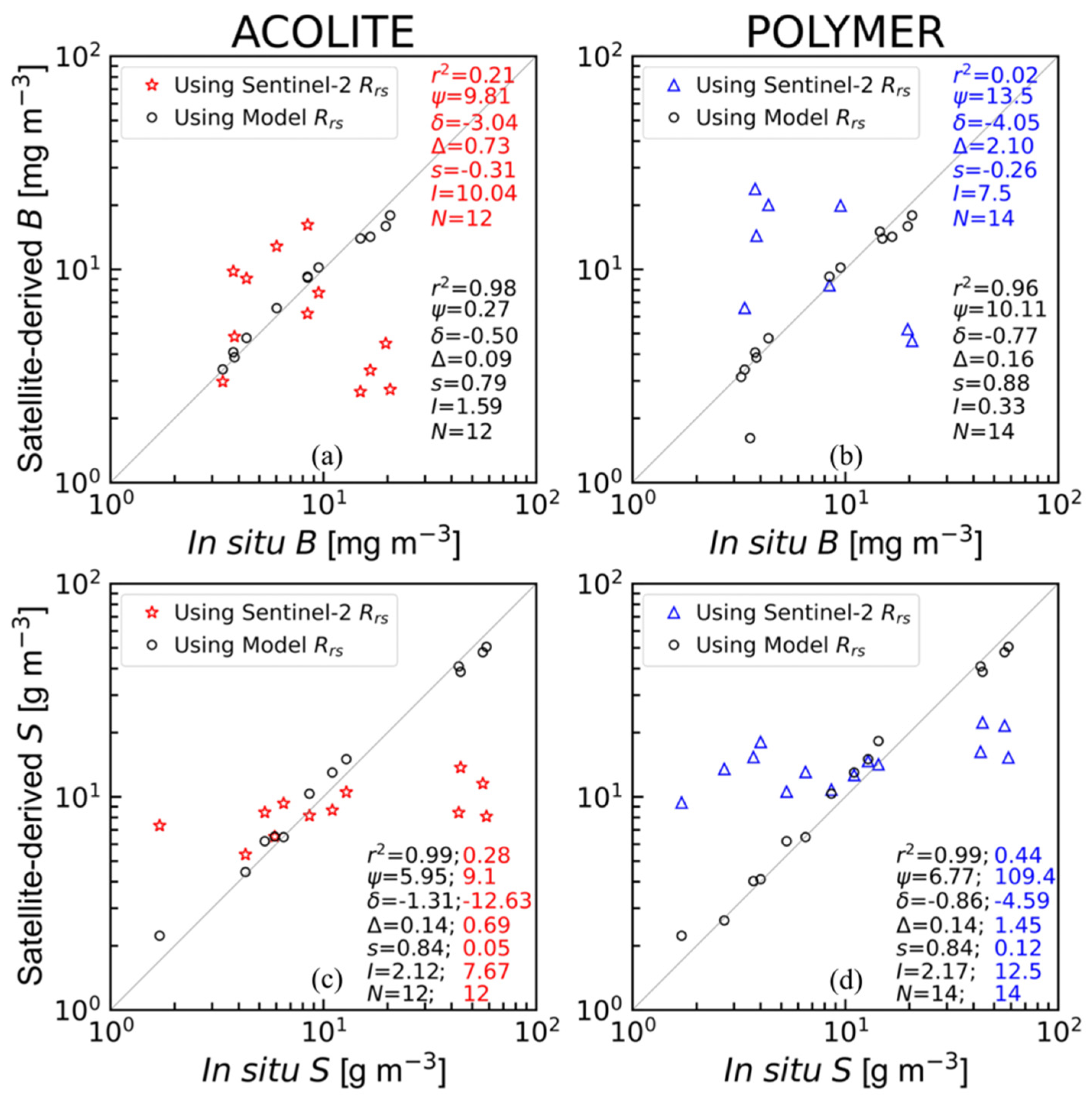
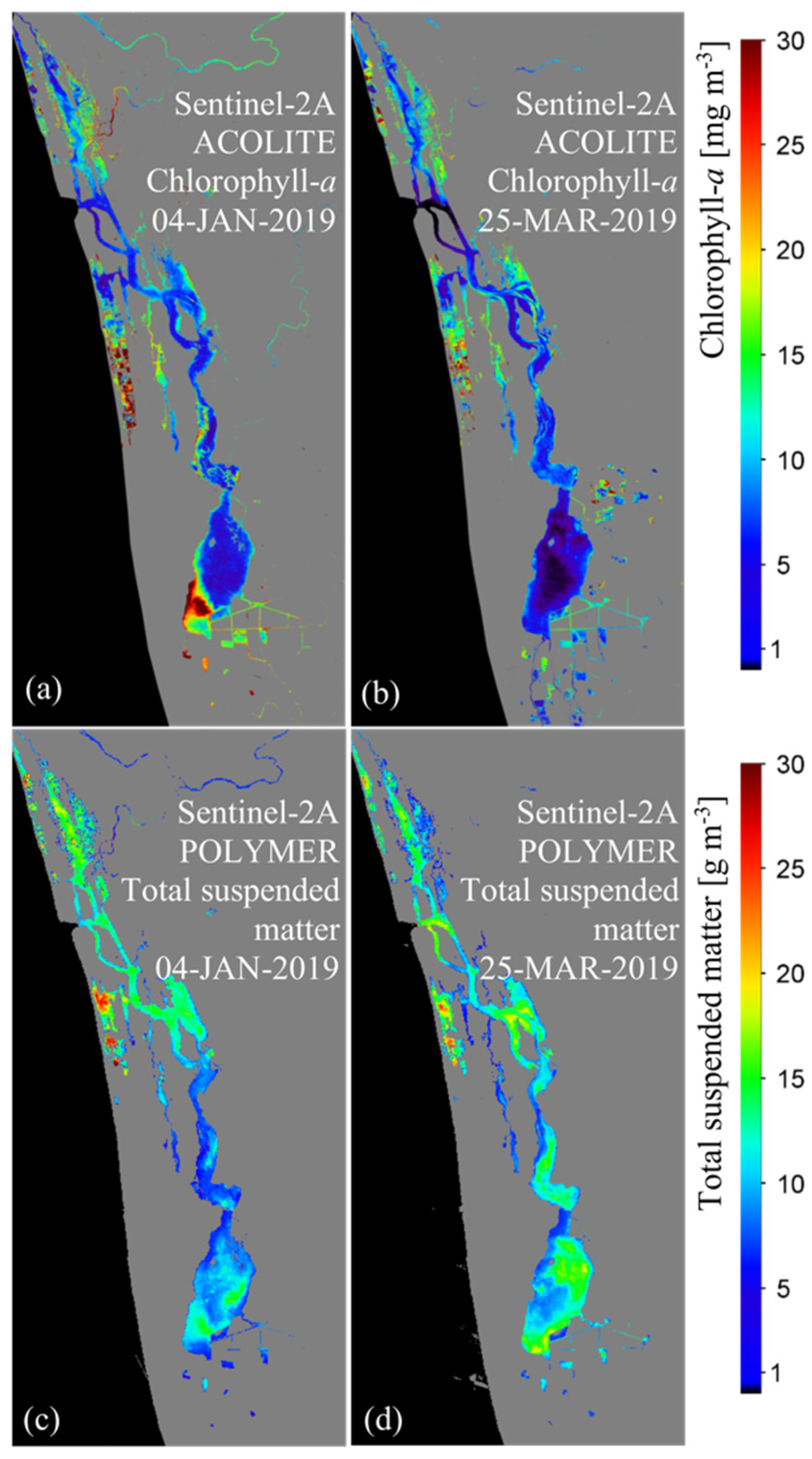
3.4. Application of Regionally Tuned Satellite Retrieval Algorithms

To identify the best atmospheric correction technique suitable for estimations of chlorophyll-a biomass ( B ) and total suspended matter ( S ) in VL, the concentrations retrieved using the empirically corrected satellite reflectance values were compared with the satellite matchup dataset (Table 1) (Figure 1). The regionally tuned Algorithms B4 and S3 were used for the retrieval of B and S , respectively. Statistical analysis demonstrated that the satellite-based B from the ACOLITE-processed data and the satellite-based S from the POLYMER-processed data compared best with in situ measurements (Figure 8a,d). We note that the estimates of B and S in both ACOLITE- and POLYMER-processed data demonstrated four outliers, all of them for samples collected on the 4th of January 2019 (Figure 8a,b). For these matchups, the corresponding in situ S values are much higher than for other samples. The reason for this anomaly remains unclear.
As examples of products that can be derived from the regionally tuned algorithms developed in this study, we demonstrate the spatial distribution of satellite-derived B and S in VL for the 4th of January and the 25th of March 2019 (Figure 9). We observe that B ranged from 3–15 mg m−3 across the lake, with occasionally higher concentrations up to 60–80 mg m−3 in the north (Figure 9a,b), and concentrations between 6–9 mg m−3 near the Thanneermukkom Bund. Concentrations of S ranged from 9–15 g m−3 on the 4th of January 2019 (Figure 9c). A maximum concentration of S of nearly 45 g m−3 was observed for some pixels, especially near Kochi and the south of the lake on the 25th of March 2019 (Figure 9d). High values of B and S in the southeast side of VL may be related to nutrient and sediment inputs from the adjacent paddy fields.

4. Discussion

4.1. Satellite Products for Sustainable Development Goals

For decades, Vembanad Lake has been impacted by anthropogenic stresses that affect its ecological health and socioeconomic status [25,74,75]. To move towards the sustainable use of Vembanad Lake, a detailed water quality monitoring programme is required [8,76,77]. In this study, we addressed the estimation of two key indicators of water quality, chlorophyll-a and total suspended matter, from remote sensing observations to support such a monitoring programme. As an indicator of ecosystem health, chlorophyll-a concentration can be used to study phytoplankton dynamics in general as well as to monitor harmful algal blooms resulting from eutrophication that affect ecosystem health [78,79]. The total suspended matter affects the turbidity of the lake with high concentrations leading to reduced light penetration, and hence decreasing the light available for photosynthesis by phytoplankton. Earlier studies in other regions have reported that high levels of S can also affect zooplankton and fish survival [80]. Satellite-based routine monitoring of these variables for the assessment of water quality can be efficient and cost-effective compared with in situ observations. For instance, there are studies that assessed the variability in water quality during the COVID-19 lockdown using satellite data in Vembanad Lake and other aquatic systems in India [41,42,81]. However, the assessment of water quality using satellite data can be improved when complementary in situ observations are available, as was the case in this study.

4.2. Challenges with Quantitative Water Quality Measurements from Satellites over Vembanad Lake

Although our study relied on an extensive field campaign in Vembanad Lake that measured various water quality indicators over an annual cycle, only a small number of matchup data points were available. Matching satellite and in situ data in Vembanad Lake was difficult because: (i) logistical issues and other conflicting requirements affected the scheduling of field campaigns during satellite overpasses, even though Sentinel-2 has a high overpass frequency of 5 days; (ii) carrying out simultaneous in situ measurements at 13 stations spread across the 100 km length of the lake is difficult; in fact, it took 2 days to complete one transect; and (iii) frequent cloud cover, especially during the monsoon seasons, limited satellite retrievals. Therefore, we employed a modelling approach to estimate the reflectance values based on IOPs that were either observed or estimated from in situ observations. The simulated reflectances constituted a large dataset (N = 162, VL dataset) that could be used to improve satellite algorithms. Using this approach, we demonstrated that the locally tuned algorithms performed better than previously established models [33,36,38,39] for the satellite retrievals of the concentrations of B and S (discussed later in this section).
The geometry of Vembanad Lake, which is long and narrow, with a highly indented shoreline and multiple waterways; the proximity to land and the potential for water-pixel contamination by neighbouring pixels; and above all, the optically complex nature of the waters; all rendered the study area particularly problematic from a remote-sensing point of view. The spatial resolution of satellite sensors such as the Ocean Colour and Land Imager (OLCI) on Sentinel-3 (300 m) was insufficient to resolve the spatial distribution of water quality properties in the lake. The solution was to make use of the MultiSpectral Instrument (MSI) on Sentinel-2, which is designed primarily for land applications, but has a spatial resolution of 10m in the visible domain. While the spatial resolution was ideal for the purposes of the study, we had to compromise on the spectral quality and resolution, and adapt in-water algorithms for the application with MSI data.
Phytoplankton-size-based models have been demonstrated to be useful in reproducing the spectral values of the absorption coefficient of phytoplankton [61,62,82,83,84,85]. Although the size-class model of Brewin et al. [61,62] worked well in the estimation of a B λ values for our study site, we recognise that the absorption values of non-algal suspended particles vary with sediment type, composition, and concentration [86,87] and, consequently, with aquatic environments [88]. For a Y , the model values demonstrated some scatter in the longer bands, especially for samples from the VL waters (Figure 4). The use of a constant slope for the absorption spectrum of yellow substances ( Y ) is known to produce high errors at long wavelengths when concentrations of Y are high or when different sources contribute to Y [89]. Previous studies have reported that the slope of a Y can vary between 0.01 and 0.02 with the composition and source of the substance [64,65,90,91,92,93]. This is also potentially true for VL, where phytoplankton, macrophytes, and materials of terrestrial origin from river runoff could all contribute to the dissolved organic matter in the water. However, the overall effect of the deviation in a Y on total absorption is minimal, since concentrations of Y are low in VL compared with B and S .
The atmospheric correction of Sentinel-2 data was another challenge. In addition to the complex nature of the water body itself, problems associated with poor air quality, high aerosol content, and high humidity, which could also have affected the aerosol properties, eventually makes it difficult to perform the atmospheric correction. We therefore implemented two well-known atmospheric correction procedures that are known to perform well in complex situations [66,94,95]. Reflectance values retrieved using both procedures—ACOLITE and POLYMER—demonstrated a significant offset when compared with simulated in situ reflectances, and the data needed a spectral bias correction to bring the magnitudes and spectral shapes to within reasonable values. Though the underlying cause responsible for the offset remains unknown, one might speculate that the algorithms were unable to distinguish fully between high aerosols in air and scattering particles in water.

4.3. Chlorophyll-a and Total Suspended Matter in Vembanad Lake

For estimating chl-a, one of the algorithms tested here was the blue-green algorithm of O’Reilly et al. [33], which is designed for use in open-ocean, Case-1 waters, where phytoplankton and chl-a can be treated as the primary agents responsible for variations in optical properties, with other substances, when present, covarying with chl-a. The poor performance of this algorithm is therefore expected in Case-2 waters, such as those of Vembanad Lake, where high absorption and scattering by particulate and dissolved organic matter, varying independently of phytoplankton, can degrade algorithm performance.
Mittenzwey et al. [34] and Gitelson [96], among others, proposed using the NIR reflectance bands, which contain information on phytoplankton, to estimate chl-a in turbid, but productive waters. The NIR chlorophyll-a algorithm of Gilerson et al. [36], after tuning for Vembanad Lake (Algorithm B3), performed well at high concentrations. At low chl-a concentrations, the phytoplankton signal is generally weak in the NIR region, introducing noise in the algorithm estimates. The conditions in Vembanad Lake called for an algorithm that works well in Case 2 environments, at both low and high chl-a concentrations. The multi-linear regression algorithm (Algorithm B4), which uses a combination of the five reflectance bands, performed effectively in the retrieval of B with high accuracy in VL waters. However, the use of short (blue and green) wavebands in satellite retrieval algorithms can also be problematic, as the reflectances at these bands are often erroneous after atmospheric corrections [97]. Hence, the performance of the multi-band algorithm should also be tested frequently and modified accordingly, as more validation data become available.
Sathyendranath et al. [68], Miller and McKee [38] and Nechad et al. [39], and others have demonstrated that reflectances in the red wavebands are suitable for the retrieval of the total suspended matter concentration. Following these earlier studies, we chose to estimate S as a function of reflectance at 665 nm, because there is a proportional increase in reflectance at this band, with an increase in S . However, the model coefficients needed to be tuned for Vembanad Lake to improve the quantitative retrieval. The need for re-parameterising the model may be attributed to the impact of the size, shape, and nature of the inorganic suspended particles on their optical properties [86,87]. Classifying the pixels into water types and applying class-specific algorithms [66,98] could be a potential avenue, to avoid the need for re-parameterising algorithms for different regions. However, the lack of b b measurements from the study site did not allow us to explore such algorithms in our study.

5. Conclusions

In this study, we presented site-specific products for chlorophyll-a and total suspended matter concentrations in Vembanad Lake, derived using high-spatial-resolution Sentinel-2 data. To this end, remote-sensing reflectances were simulated using a forward modelling approach that uses absorption, and back-scattering coefficients as inputs. Then, the simulated reflectances were used to test algorithms for estimating the chlorophyll-a biomass ( B ) and total suspended matter ( S ) concentrations. We used the NOMAD and Vembanad Lake in situ datasets for developing the reflectance model and for validation. Two different atmospheric correction techniques—ACOLITE and POLYMER—were examined for the application of regionally tuned chlorophyll-a and total suspended matter algorithms in Vembanad Lake. The satellite-retrieved products were validated against in situ matchups. When compared with other commonly-used algorithms, in situ data and values estimated from the site-specific algorithms proposed in the current study were in good agreement despite the fact that the number of matchups was small. Although ACOLITE and POLYMER atmospheric correction procedures produced similar results, we recommend the use of ACOLITE-based reflectances for the estimation of chlorophyll-a and POLYMER-based reflectances for the estimation of total suspended matter concentrations. The statistical performance of both ACOLITE and POLYMER were comparable for the retrieval of total suspended matter concentration; POLYMER had a small advantage with respect to spatial coverage. This study indicates that the algorithms developed here can be used for the routine monitoring of water quality in the management of Vembanad Lake, which is valuable in the assessment of the effects of anthropogenic activities on human and aquatic life. In particular, the satellite-derived chlorophyll-a, when combined with photosynthetically available radiation (PAR), can support studies related to primary production. Systematic studies of chlorophyll-a concentration are also useful for monitoring phytoplankton blooms, including harmful algal blooms. A recent study also demonstrated [22] that there is a complex relationship between chlorophyll-a concentration and the presence of Vibrio cholerae bacteria in Vembanad Lake. Sediment dynamics, critical for the local harbour, can now be monitored from the satellite, and could help investigate the impact of dredging activities to maintain the water depth in shipping channels. Furthermore, such observations can be used to infer the flushing rate of water in the lacustrine–estuarine system, a critical component among various factors that maintain the health of the lake ecosystem. Such observations can also help to monitor erosion and deposition along the shoreline. Thus, this study supports the United Nation’s sustainable development goals—3, 6, and 14 by monitoring the water quality and by helping to maintain good human and animal health both in water and along the shores of Vembanad Lake. Future efforts include calibrating the model coefficients with more satellite matchups; implementing an improved atmospheric correction method; using in situ back-scattering coefficients and eliminating uncertainties associated with using a constant bidirectional factor (f/Q), which could help in enhancing the model performance.

Author Contributions

Conceptualization, V.T. and S.S.; methodology: V.T., S.S., G.K., N.S., N.M., G.G., A.A. and R.J.W.B.; software: V.T., G.K. and N.S.; validation: V.T., S.S., G.K., N.M., G.G., A.A. and R.J.W.B.; formal analysis: V.T., S.S. and G.K.; investigation: V.T., S.S., G.K., N.S., N.M., G.G., A.A. and R.J.W.B.; resources: S.S., T.P., R.J.W.B., N.M., G.G. and A.A.; data curation: V.T., G.K., N.S., N.M., G.G., A.A., A.R. and S.X.; writing—original draft preparation: V.T., S.S. and G.K.; writing—review and editing: All authors. visualization: V.T. and G.K.; supervision: S.S. and T.P.; project administration: A.A., G.G., N.M. and S.S.; funding acquisition: S.S., T.P., R.J.W.B., A.A. and G.G. All authors have read and agreed to the published version of the manuscript.

Funding

This research was funded under the project REVIVAL by the Natural Environmental Research Council (UK) and the Department of Science and Technology, India (DST/TM/INDOUK/2K17/64 (C) as part of the India-UK water quality research programme. This research was also funded by the European Space Agency (ESA) under the WIDGEON and Dragon projects. This work is a contribution to the activities of National Centre for Earth Observation (NCEO) of the UK Natural Environmental Research Council. R.J.W.B. is supported by a UKRI Future Leader Fellowship (MR/V022792/1).

Data Availability Statement

Data available with the corresponding author. Would be shared on request.

Acknowledgments

This work is dedicated to the memory of Trevor Platt, our co-author, mentor, and inspiration. This is a contribution to the activities of the National Centre for Earth Observations of the Natural Environment Research Council (UK). We acknowledge CSIR-NIO, ICAR-CMFRI, NERCI, PML, and Scientist-in-Charge of CSIR-NIO RCK for their support and encouragement.

Conflicts of Interest

The authors declare no conflict of interest.

Appendix A

Table A1. Notations, their descriptions, and units used in the present study.
NotationsDescriptionUnits
a Absorption coefficientm−1
a B Absorption coefficient of phytoplanktonm−1
a m Absorption coefficient of microphytoplanktonm−1
a m * Chlorophyll-specific absorption coefficient of microphytoplanktonm2 (mg chl-a)−1
a n Absorption coefficient of nanophytoplanktonm−1
a n * Chlorophyll-specific absorption coefficient of nanophytoplanktonm2 (mg chl-a)−1
a p Absorption coefficient of picophytoplanktonm−1
a p * Chlorophyll-specific absorption coefficient of picophytoplanktonm2 (mg chl-a)−1
a S Absorption coefficient of non-algal suspended particlesm−1
a B + S Absorption coefficient of particulate matter (phytoplankton biomass + non-algal suspended particles)m−1
a t Total absorption coefficientm−1
a W Absorption coefficient of waterm−1
a Y Absorption coefficient of coloured dissolved organic matter, or yellow matterm−1
A ACOLITE-
b b Back-scattering coefficientm−1
b b S Back-scattering coefficient of non-algal suspended particlesm−1
b b S * Specific-back-scattering coefficient of non-algal suspended particlesm2 g−1
b b t Total back-scattering coefficientm−1
b b W Back-scattering coefficient of waterm−1
B Phytoplankton biomass, in units of chlorophyll-amg m−3
B m Microphytoplankton biomass, in units of chlorophyll-amg chl-a m−3
B n Nanophytoplankton biomass, in units of chlorophyll-amg chl-a m−3
B p Picophytoplankton biomass, in units of chlorophyll-amg chl-a m−3
B p , n Combined pico- and nanophytoplankton biomass, in units of chlorophyll-amg chl-a m−3
B p , n m Asymptotic maximum value of combined pico- and nanophytoplankton biomass, in units of chlorophyll-amg chl-a m−3
B p m Asymptotic maximum value of picophytoplankton biomass, in units of chlorophyll-amg chl-a m−3
D Optical densityDimensionless
D B Optical density of phytoplankton biomassDimensionless
D S Optical density of non-algal suspended particlesDimensionless
D B + S Optical density of particulate matter (phytoplankton biomass + non-algal suspended particles)Dimensionless
D Y Optical density of coloured dissolved organic matterDimensionless
E s Downwelling surface irradianceμW cm−2 nm−1
f A proportional constant for IOP-based reflectance-
I Intercept values estimated between measured and modelled data-
k Spectral slope of back-scattering coefficient of non-algal suspended particlesDimensionless
L w Water-leaving radianceμW cm−2 nm−1 sr−1
m Fitted coefficientsDimensionless
m S Spectral slope of absorption coefficient of non-algal suspended particlesnm−1
m Y Spectral slope of absorption coefficient of coloured dissolved organic matternm−1
N Number of samples-
P POLYMER-
Q Bi-directional factorsr
R ReflectanceDimensionless
R i In situ irradiance reflectanceDimensionless
R e Estimated/Modelled reflectanceDimensionless
R r s Remote-sensing reflectancesr−1
r 2 Determination coefficient-
S Total suspended matterg m−3
s Slope values estimated between measured and modelled data-
S p Slope to estimate picophytoplankton biomassDimensionless
S p , n Slope to estimate combined pico- and nanophytoplankton biomassDimensionless
W Notation for water-
Y Notation for coloured dissolved organic matter, or yellow substances-
δ Bias-
Δ Mean relative error-
λ Wavelengthnm
ρ w Water-leaving reflectance (referred to as ‘satellite reflectance’ when it is derived from satellite)Dimensionless
ρ w A Uncorrected ACOLITE-based satellite reflectanceDimensionless
ρ w P Uncorrected POLYMER-based satellite reflectanceDimensionless
ρ w Corrected satellite reflectanceDimensionless
ρ w A Corrected ACOLITE-based satellite reflectanceDimensionless
ρ w P Corrected POLYMER-based satellite reflectanceDimensionless
ψ Root mean square error-
Figure A1. The tuned correction coefficients m A (ACOLITE) (a) and m P (POLYMER) (b) that were used to correct for the difference between the satellite ( ρ w ) and modelled reflectance R e .
Remotesensing 14 06404 g0a1
Figure A2. The ranges of B (a) and S (b) from the NOMAD and Vembanad Lake datasets used in the present study. The dashed lines in both plots represent the ranges of B (0.2~57 [mg m−3]) and S (0.13~43.1 [g m−3]) used to derive b b S 665 vs. S relation [66].
Remotesensing 14 06404 g0a2
Figure A3. Spectral comparisons of modelled ( R e first column), uncorrected satellite-observed ( ρ w , second column), and corrected satellite-observed ( ρ w , third column) reflectances. The insets show the reflectance spectra of ρ w A (b) and ρ w P (e) at smaller scales to demonstrate their actual magnitude and spectral features.
Remotesensing 14 06404 g0a3

References

  1. Cole, J.J.; Caraco, N.F. Carbon in Catchments: Connecting Terrestrial Carbon Losses with Aquatic Metabolism. Mar. Freshw. Res. 2001, 52, 101–110. [Google Scholar] [CrossRef] [Green Version]
  2. Sobek, S.; Algesten, G.; Bergström, A.K.; Jansson, M.; Tranvik, L.J. The Catchment and Climate Regulation of PCO2 in Boreal Lakes. Glob. Chang. Biol. 2003, 9, 630–641. [Google Scholar] [CrossRef]
  3. Bastviken, D.; Cole, J.; Pace, M.; Tranvik, L. Methane Emissions from Lakes: Dependence of Lake Characteristics, Two Regional Assessments, and a Global Estimate. Glob. Biogeochem. Cycles 2004, 18, 1–12. [Google Scholar] [CrossRef]
  4. Raymond, P.A.; Hartmann, J.; Lauerwald, R.; Sobek, S.; McDonald, C.; Hoover, M.; Butman, D.; Striegl, R.; Mayorga, E.; Humborg, C.; et al. Global Carbon Dioxide Emissions from Inland Waters. Nature 2013, 503, 355–359. [Google Scholar] [CrossRef] [PubMed] [Green Version]
  5. Schallenberg, M.; De Winton, M.D.; Verburg, P.; Kelly, D.J.; Hamill, K.D.; Hamilton, D.P. Ecosystem Services of Lakes. Ecosyst. Serv. N. Z. Cond. Trends 2013, 203–225. Available online: https://www.cabdirect.org/cabdirect/abstract/20143064097 (accessed on 13 November 2022).
  6. Jorgensen, S.E.; Loffler, H.; Rast, W.; Straskraba, M. Lake and Reservoir Management; Elsevier: Amsterdam, The Netherlands, 2005. [Google Scholar]
  7. Beiras, R. Marine Pollution: Sources, Fate and Effects of Pollutants in Coastal Ecosystems; Elsevier: Amsterdam, The Netherlands, 2018. [Google Scholar]
  8. UN Environment Global Manual on Ocean Statistics. Towards a Definition of Indicator Methodologies; UN Environment: Nairobi, Kenya, 2018; p. 46. Available online: https://wesr.unep.org/media/docs/statistics/egm/global_manual_on_ocean_statistics_towards_a_definition_of_indicator_methodologies.pdf (accessed on 11 November 2022).
  9. Häder, D.P.; Banaszak, A.T.; Villafañe, V.E.; Narvarte, M.A.; González, R.A.; Helbling, E.W. Anthropogenic Pollution of Aquatic Ecosystems: Emerging Problems with Global Implications. Sci. Total Environ. 2020, 713, 136586. [Google Scholar] [CrossRef] [PubMed]
  10. Barboza, L.G.A.; Dick Vethaak, A.; Lavorante, B.R.B.O.; Lundebye, A.K.; Guilhermino, L. Marine Microplastic Debris: An Emerging Issue for Food Security, Food Safety and Human Health. Mar. Pollut. Bull. 2018, 133, 336–348. [Google Scholar] [CrossRef]
  11. Guterres, A. The Sustainable Development Goals Report 2020; United Nations Department of Economic and Social Affairs: New York, NY, USA, 2021; pp. 1–64. Available online: https://unstats.un.org/sdgs/report/2021/The-Sustainable-Development-Goals-Report-2021.pdf (accessed on 11 November 2022).
  12. Jaramillo, F.; Desormeaux, A.; Hedlund, J.; Jawitz, J.W.; Clerici, N.; Piemontese, L.; Rodríguez-Rodriguez, J.A.; Anaya, J.A.; Blanco-Libreros, J.F.; Borja, S.; et al. Priorities and Interactions of Sustainable Development Goals (SDGs) with Focus on Wetlands. Water 2019, 11, 619. [Google Scholar] [CrossRef] [Green Version]
  13. Ho, L.T.; Goethals, P.L.M. Opportunities and Challenges for the Sustainability of Lakes and Reservoirs in Relation to the Sustainable Development Goals (SDGs). Water 2019, 11, 1462. [Google Scholar] [CrossRef] [Green Version]
  14. Cicin-Sain, B. Sustainable Development and Integrated Coastal Management. Ocean Coast. Manag. 1993, 21, 11–43. [Google Scholar] [CrossRef]
  15. Pfeiffer, W.C.; Drude de Lacerda, L.; Malm, O.; Souza, C.M.M.; da Silveira, E.G.; Bastos, W.R. Mercury Concentrations in Inland Waters of Gold-Mining Areas in Rondônia, Brazil. Sci. Total Environ. 1989, 87–88, 233–240. [Google Scholar] [CrossRef] [PubMed]
  16. Allan, J.D.; Abell, R.; Hogan, Z.; Revenga, C.; Taylor, B.W.; Welcomme, R.L.; Winemiller, K. Overfishing of Inland Waters. Bioscience 2005, 55, 1041–1051. [Google Scholar] [CrossRef] [Green Version]
  17. González Farias, F.A.; Hernández-Garza, M.D.R.; Díaz González, G. Organic Carbon and Pesticide Pollution in a Tropical Coastal Lagoon-Estuarine System in Northwest Mexico. Int. J. Environ. Pollut. 2006, 26, 234–253. [Google Scholar] [CrossRef]
  18. Santiago-Rodriguez, T.M.; Tremblay, R.L.; Toledo-Hernandez, C.; Gonzalez-Nieves, J.E.; Ryu, H.; Santo Domingo, J.W.; Toranzosa, G.A. Microbial Quality of Tropical Inland Waters and Effects of Rainfall Events. Appl. Environ. Microbiol. 2012, 78, 5160–5169. [Google Scholar] [CrossRef] [Green Version]
  19. Majozi, N.P.; Salama, M.S.; Bernard, S.; Harper, D.M.; Habte, M.G. Remote Sensing of Euphotic Depth in Shallow Tropical Inland Waters of Lake Naivasha Using MERIS Data. Remote Sens. Environ. 2014, 148, 178–189. [Google Scholar] [CrossRef]
  20. Balachandran, K.K. Ecosystem Modeling of the Vembanad Lake (Cochin Backwaters); Workshop on Indian Estuaries, National Institute of Oceanography: Dona Paula, India, 2007; pp. 16–18. [Google Scholar]
  21. Ramamurthy, T.; Sharma, N.C. Cholera Outbreaks in India Thandavarayan. Curr. Top. Microbiol. Immunol. 2014, 379, 49–85. [Google Scholar] [CrossRef]
  22. Anas, A.; Krishna, K.; Vijayakumar, S.; George, G.; Menon, N.; Kulk, G.; Chekidhenkuzhiyil, J.; Ciambelli, A.; Kuttiyilmemuriyil Vikraman, H.; Tharakan, B.; et al. Dynamics of Vibrio Cholerae in a Typical Tropical Lake and Estuarine System: Potential of Remote Sensing for Risk Mapping. Remote Sens. 2021, 13, 1034. [Google Scholar] [CrossRef]
  23. Sathyendranath, S.; Abdulaziz, A.; Menon, N.; George, G.; Evers-King, H.; Kulk, G.; Colwell, R.; Jutla, A.; Platt, T. Building Capacity and Resilience against Diseases Transmitted via Water under Climate Perturbations and Extreme Weather Stress. In Space Capacity Building in the XXI Century; Ferretti, S., Ed.; Springer: Cham, Switzerland, 2020; pp. 281–298. [Google Scholar]
  24. Reed, R.H.; Singh, B.; Mani, S.K. Solar Disinfection of Drinking Water: Lessons from Field Studies in India. In Progress on Drinking Water Research; Lefebvre, M.H., Roux, M.M., Eds.; Nova Science Publishers, Inc.: New York, NY, USA, 2008; Volume 1, 290p. [Google Scholar]
  25. Menon, N.N.; Balchand, A.N.; Menon, N.R. Hydrobiology of the Cochin Backwater System—A Review. Hydrobiologia 2000, 430, 149–183. [Google Scholar] [CrossRef]
  26. Ramasamy, E.V.; Jayasooryan, K.K.; Chandran, M.S.S.; Mohan, M. Total and Methyl Mercury in the Water, Sediment, and Fishes of Vembanad, a Tropical Backwater System in India. Environ. Monit. Assess. 2017, 189, 1–19. [Google Scholar] [CrossRef]
  27. Sruthy, S.; Ramasamy, E.V. Microplastic Pollution in Vembanad Lake, Kerala, India: The First Report of Microplastics in Lake and Estuarine Sediments in India. Environ. Pollut. 2017, 222, 315–322. [Google Scholar] [CrossRef] [PubMed]
  28. Jose, J.; Giridhar, R.; Anas, A.; Loka Bharathi, P.A.; Nair, S. Heavy Metal Pollution Exerts Reduction/Adaptation in the Diversity and Enzyme Expression Profile of Heterotrophic Bacteria in Cochin Estuary, India. Environ. Pollut. 2011, 159, 2775–2780. [Google Scholar] [CrossRef] [PubMed]
  29. Sheeba, V.A.; Abdulaziz, A.; Gireeshkumar, T.R.; Ram, A.; Rakesh, P.S.; Jasmin, C.; Parameswaran, P.S. Role of Heavy Metals in Structuring the Microbial Community Associated with Particulate Matter in a Tropical Estuary. Environ. Pollut. 2017, 231, 589–600. [Google Scholar] [CrossRef] [PubMed]
  30. Sudhi, K.S. Vembanad Route to Track CRZ Violations in Kerala. Available online: https://www.thehindu.com/news/national/kerala/vembanad-route-to-track-crz-violations-in-state/article29493876.ece (accessed on 11 November 2022).
  31. Menon, N.; George, G.; Ranith, R.; Sajin, V.; Murali, S.; Abdulaziz, A.; Brewin, R.J.W.; Sathyendranath, S. Citizen Science Tools Reveal Changes in Estuarine Water Quality Following Demolition of Buildings. Remote Sens. 2021, 13, 1683. [Google Scholar] [CrossRef]
  32. George, G.; Menon, N.N.; Abdulaziz, A.; Brewin, R.J.W.; Pranav, P.; Gopalakrishnan, A.; Mini, K.G.; Kuriakose, S.; Sathyendranath, S.; Platt, T. Citizen Scientists Contribute to Real-Time Monitoring of Lake Water Quality Using 3D Printed Mini Secchi Disks. Front. Water 2021, 3, 1–14. [Google Scholar] [CrossRef]
  33. O’Reilly, J.E.; Maritorena, S.; O’brien, M.C.; Siegel, D.A.; Toole, D.; Menzies, D.; Smith, R.C.; Mueller, J.L.; Mitchell, B.G.; Kahru, M.; et al. SeaWiFS Postlaunch Calibration and Validation Analyses, Part 3; Hooker, S.B., Firestone, E.R., Eds.; SeaWiFS Postlaunch Technical Report Series; NASA: Washington, DC, USA, 2000; p. 51.
  34. Mittenzwey, K.H.; Ullrich, S.; Gitelson, A.A.; Kondratiev, K.Y. Determination of Chlorophyll-a of Inland Waters on the Basis of Spectral Reflectance. Limnol. Oceanogr. 1992, 37, 147–149. [Google Scholar] [CrossRef]
  35. Gons, H.J. Optical Teledetection of Chlorophyll a in Turbid Inland Waters. Environ. Sci. Technol. 1999, 33, 1127–1132. [Google Scholar] [CrossRef]
  36. Gilerson, A.A.; Gitelson, A.A.; Zhou, J.; Gurlin, D.; Moses, W.; Ioannou, I.; Ahmed, S.A. Algorithms for Remote Estimation of Chlorophyll-a in Coastal and Inland Waters Using Red and near Infrared Bands. Opt. Express 2010, 18, 24109–24125. [Google Scholar] [CrossRef] [Green Version]
  37. Mishra, S.; Mishra, D.R. Normalized Difference Chlorophyll Index: A Novel Model for Remote Estimation of Chlorophyll-a Concentration in Turbid Productive Waters. Remote Sens. Environ. 2012, 117, 394–406. [Google Scholar] [CrossRef]
  38. Miller, R.L.; McKee, B.A. Using MODIS Terra 250 m Imagery to Map Concentrations of Total Suspended Matter in Coastal Waters. Remote Sens. Environ. 2004, 93, 259–266. [Google Scholar] [CrossRef]
  39. Nechad, B.; Ruddick, K.G.; Park, Y. Calibration and Validation of a Generic Multisensor Algorithm for Mapping of Total Suspended Matter in Turbid Waters. Remote Sens. Environ. 2010, 114, 854–866. [Google Scholar] [CrossRef]
  40. Avtar, R.; Kumar, P.; Supe, H.; Jie, D.; Sahu, N.; Mishra, B.K.; Yunus, A.P. Did the COVID-19 Lockdown-Induced Hydrological Residence Time Intensify the Primary Productivity in Lakes? Observational Results Based on Satellite Remote Sensing. Water 2020, 12, 2573. [Google Scholar] [CrossRef]
  41. Kulk, G.; George, G.; Abdulaziz, A.; Menon, N.; Theenathayalan, V.; Jayaram, C.; Brewin, R.J.W.; Sathyendranath, S. Effect of Reduced Anthropogenic Activities on Water Quality in Lake Vembanad, India. Remote Sens. 2021, 13, 1631. [Google Scholar] [CrossRef]
  42. Yunus, A.P.; Masago, Y.; Hijioka, Y. COVID-19 and Surface Water Quality: Improved Lake Water Quality during the Lockdown. Sci. Total Environ. 2020, 731, 139012. [Google Scholar] [CrossRef]
  43. Lakshmanan, P.T.; Shynamma, C.S.; Balchand, A.N.; Kurup, P.G. Distribution and Seasonal Variation of Temperature and Salinity in Cochin Backwaters [West India]. Deep Sea Res. Part B. Oceanogr. Lit. Rev. 1982, 29, 750. [Google Scholar] [CrossRef]
  44. Kishino, M. Estimation of Quantum Yield of Chlorophyll a Fluorescence from the Upward Irradiance Spectrum in the Sea. La Mer 1984, 22, 233–240. [Google Scholar]
  45. Ferrari, G.M.; Dowell, M.D.; Grossi, S.; Targa, C. Relationship between the Optical Properties of Chromophoric Dissolved Organic Matter and Total Concentration of Dissolved Organic Carbon in the Southern Baltic Sea Region. Mar. Chem. 1996, 55, 299–316. [Google Scholar] [CrossRef]
  46. Mitchell, B.G.; Kahru, M.; Wieland, J.; Stramska, M. Determination of Spectral Absorption Coefficients of Particles, Dissolved Material and Phytoplankton for Discrete Water Samples. Ocean Opt. Protoc. Satell. Ocean Color Sens. Valid. Revis. 2003, 4, 39–64. [Google Scholar]
  47. Shanmugam, P. New Models for Retrieving and Partitioning the Colored Dissolved Organic Matter in the Global Ocean: Implications for Remote Sensing. Remote Sens. Environ. 2011, 115, 1501–1521. [Google Scholar] [CrossRef]
  48. Mitchell, B.G. Algorithms for Determining the Absorption Coefficient for Aquatic Particulates Using the Quantitative Filter Technique. In Ocean Optics X; International Society for Optics and Photonics: Bellingham, WA, USA, 1990; Volume 1302, pp. 137–148. [Google Scholar]
  49. Jerlov, N.G. Marine Optics; Elsevier: Amsterdam, The Netherlands, 1976; Volume 14. [Google Scholar]
  50. Kirk, J.T.O. Light and Photosynthesis in Aquatic Ecosystems; Cambridge University Press: Cambridge, UK, 1994. [Google Scholar]
  51. Parsons, T.R.; Maita, Y.; Lalli, C.M. A Manual of Chemical and Biological Methods for Sea Water Analysis; Pergamon Press: Oxford, UK, 1984; Volume 31, ISBN 0080302882. [Google Scholar]
  52. Jeffrey, S.W.; Humphrey, G.F. New Spectrophotometric Equations for Determining Chlorophylls a, b, C1 and C2 in Higher Plants, Algae and Natural Phytoplankton. Biochem. Physiol. Pflanz. 1975, 167, 191–194. [Google Scholar] [CrossRef]
  53. Strickland, J.D.H.; Parsons, T.R. A Practical Handbook of Seawater Analysis, 2nd ed.; Fisheries Research Board of Canada: Ottawa, ON, Canada, 1972; 310p, Available online: https://repository.oceanbestpractices.org/handle/11329/1994 (accessed on 13 November 2022).
  54. Tilstone, G.H.; Martinez-Vicente, V. ISECA Protocols for the Validation of Ocean Colour Satellite Data in Case 2 European Waters; Plymouth Marine Laboratory (PML): Plymouth, UK, 2012. [Google Scholar]
  55. Werdell, P.J.; Bailey, S.W. An Improved In-Situ Bio-Optical Data Set for Ocean Color Algorithm Development and Satellite Data Product Validation. Remote Sens. Environ. 2005, 98, 122–140. [Google Scholar] [CrossRef]
  56. Vanhellemont, Q.; Ruddick, K. Atmospheric Correction of Metre-Scale Optical Satellite Data for Inland and Coastal Water Applications. Remote Sens. Environ. 2018, 216, 586–597. [Google Scholar] [CrossRef]
  57. Vanhellemont, Q.; Ruddick, K. Adaptation of the Dark Spectrum Fitting Atmospheric Correction for Aquatic Applications of the Landsat and Sentinel-2 Archives. Remote Sens. Environ. 2019, 225, 175–192. [Google Scholar] [CrossRef]
  58. Steinmetz, F.; Deschamps, P.; Ramon, D. Atmospheric Correction in Presence of Sun Glint: Application to MERIS. Opt. Express 2011, 19, 9783–9800. [Google Scholar] [CrossRef]
  59. Bailey, S.W.; Werdell, P.J. A Multi-Sensor Approach for the on-Orbit Validation of Ocean Color Satellite Data Products. Remote Sens. Environ. 2006, 102, 12–23. [Google Scholar] [CrossRef]
  60. Pope, R.M.; Fry, E.S. Absorption Spectrum (380–700 Nm) of Pure Water II Integrating Cavity Measurements. Appl. Opt. 1997, 36, 8710–8723. [Google Scholar] [CrossRef]
  61. Brewin, R.J.W.; Devred, E.; Sathyendranath, S.; Lavender, S.J.; Hardman-mountford, N.J. Model of Phytoplankton Absorption Based on Three Size Classes. Appl. Opt. 2011, 50, 4535–4549. [Google Scholar] [CrossRef]
  62. Brewin, R.J.W.; Sathyendranath, S.; Jackson, T.; Barlow, R.; Brotas, V.; Airs, R.; Lamont, T. Influence of Light in the Mixed-Layer on the Parameters of a Three-Component Model of Phytoplankton Size Class. Remote Sens. Environ. 2015, 168, 437–450. [Google Scholar] [CrossRef]
  63. Bricaud, A.; Morel, A.; Prieur, L. Absorption by Dissolved Organic Matter of the Sea (Yellow Substance) in the UV and Visible Domains1. Limnol. Oceanogr. 1981, 26, 43–53. [Google Scholar] [CrossRef]
  64. Shanmugam, P. A New Bio-Optical Algorithm for the Remote Sensing of Algal Blooms in Complex Ocean Waters. J. Geophys. Res. Ocean. 2011, 116, 1–12. [Google Scholar] [CrossRef] [Green Version]
  65. Twardowski, M.S.; Boss, E.; Sullivan, J.M.; Donaghay, P.L. Modeling the Spectral Shape of Absorption by Chromophoric Dissolved Organic Matter. Mar. Chem. 2004, 89, 69–88. [Google Scholar] [CrossRef]
  66. Balasubramanian, S.V.; Pahlevan, N.; Smith, B.; Binding, C.; Schalles, J.; Loisel, H.; Gurlin, D.; Greb, S.; Alikas, K.; Randla, M.; et al. Robust Algorithm for Estimating Total Suspended Solids (TSS) in Inland and Nearshore Coastal Waters. Remote Sens. Environ. 2020, 246, 111768. [Google Scholar] [CrossRef]
  67. Morel, A. Optical Properties of Pure Water and Pure Sea Water. In Optical Aspects of Oceanography; Jerlov, N.G., Nielson, E.S., Eds.; Academic Press: New York, NY, USA, 1974; pp. 1–24. [Google Scholar]
  68. Sathyendranath, S.; Prieur, L.; Morel, A. A Three-Component Model of Ocean Colour and Its Application to Remote Sensing of Phytoplankton Pigments in Coastal Waters. Int. J. Remote Sens. 1989, 10, 1373–1394. [Google Scholar] [CrossRef]
  69. Franz, B.A.; Bailey, S.W.; Kuring, N.; Werdell, P.J. Ocean Color Measurements with the Operational Land Imager on Landsat-8: Implementation and Evaluation in SeaDAS. J. Appl. Remote Sens. 2015, 9, 1–16. [Google Scholar] [CrossRef]
  70. Vanhellemont, Q.; Ruddick, K. Acolite for Sentinel-2: Aquatic Applications of MSI Imagery. In Proceedings of the 2016 ESA Living Planet Symposium, Prague, Czech Republic, 9–13 May 2016; p. SP-740. [Google Scholar]
  71. Morel, A.; Prieur, L. Analysis of Variations in Ocean Color. Limnol. Oceanogr. 1977, 22, 709–722. [Google Scholar] [CrossRef]
  72. Sathyendranath, S.; Platt, T. Analytic Model of Ocean Color. Appl. Opt. 1997, 36, 2620. [Google Scholar] [CrossRef]
  73. Doxaran, D.; Froidefond, J.M.; Lavender, S.; Castaing, P. Spectral Signature of Highly Turbid Waters: Application with SPOT Data to Quantify Suspended Particulate Matter Concentrations. Remote Sens. Environ. 2002, 81, 149–161. [Google Scholar] [CrossRef]
  74. WISA. Conservation and Wise Use of Vemabanad-Kol: An Integrated Management Planning Framework; Wetlands International-South Asia: New Delhi, India, 2013; pp. 1–137. [Google Scholar]
  75. Narayanan, N.C.; Venot, J.P. Drivers of Change in Fragile Environments: Challenges to Governance in Indian Wetlands. Nat. Resour. Forum 2009, 33, 320–333. [Google Scholar] [CrossRef]
  76. EU. Directive 2000/60/EC of the European Parliament and of the Council Establishing a Framework for the Community Action in the Field of Water Policy. Off. J. Eur. Communities 2000, 327, 1–72. [Google Scholar]
  77. Hussain, J.; Prabhakar, R.N. Water Quality Activities in Central Water Commission; Ministry of Jal Shakti: New Delhi, India, 2020. [Google Scholar]
  78. Mishra, S.; Mishra, D.R.; Lee, Z.; Tucker, C.S. Quantifying Cyanobacterial Phycocyanin Concentration in Turbid Productive Waters: A Quasi-Analytical Approach. Remote Sens. Environ. 2013, 133, 141–151. [Google Scholar] [CrossRef]
  79. Varunan, T.; Shanmugam, P. An Optical Tool for Quantitative Assessment of Phycocyanin Pigment Concentration in Cyanobacterial Blooms within Inland and Marine Environments. J. Great Lakes Res. 2017, 43, 32–49. [Google Scholar] [CrossRef]
  80. Bilotta, G.S.; Brazier, R.E. Understanding the Influence of Suspended Solids on Water Quality and Aquatic Biota. Water Res. 2008, 42, 2849–2861. [Google Scholar] [CrossRef] [PubMed]
  81. Jayaram, C.; Roy, R.; Chacko, N.; Swain, D.; Punnana, R.; Bandyopadhyay, S.; Choudhury, S.B.; Dutta, D. Anomalous Reduction of the Total Suspended Matter During the COVID-19 Lockdown in the Hooghly Estuarine System. Front. Mar. Sci. 2021, 8, 1–11. [Google Scholar] [CrossRef]
  82. Devred, E.; Sathyendranath, S.; Stuart, V.; Maass, H.; Ulloa, O.; Platt, T. A Two-Component Model of Phytoplankton Absorption in the Open Ocean: Theory and Applications. J. Geophys. Res. 2006, 111, 1–11. [Google Scholar] [CrossRef]
  83. Devred, E.; Sathyendranath, S.; Stuart, V.; Platt, T. A Three Component Classification of Phytoplankton Absorption Spectra: Application to Ocean-Color Data. Remote Sens. Environ. 2011, 115, 2255–2266. [Google Scholar] [CrossRef]
  84. Sathyendranath, S.; Platt, T.; Cota, G.; Stuart, V. Remote Sensing of Phytoplankton Pigments: A Comparison of Empirical and Theoretical Approaches. Int. J. Remote Sens. 2001, 22, 249–273. [Google Scholar] [CrossRef]
  85. Varunan, T.; Shanmugam, P. A Model for Estimating Size-Fractioned Phytoplankton Absorption Coefficients in Coastal and Oceanic Waters from Satellite Data. Remote Sens. Environ. 2015, 158, 235–254. [Google Scholar] [CrossRef]
  86. Babin, M.; Stramski, D. Variations in the Mass-Specific Absorption Coefficient of Mineral Particles Suspended in Water. Limnol. Oceanogr. 2004, 49, 756–767. [Google Scholar] [CrossRef] [Green Version]
  87. Doxaran, D.; Ruddick, K.; McKee, D.; Gentili, B.; Tailliez, D.; Chami, M.; Babin, M. Spectral Variations of Light Scattering by Marine Particles in Coastal Waters, from Visible to near Infrared. Limnol. Oceanogr. 2009, 54, 1257–1271. [Google Scholar] [CrossRef] [Green Version]
  88. Werdell, P.J.; McKinna, L.I.W.; Boss, E.; Ackleson, S.G.; Craig, S.E.; Gregg, W.W.; Lee, Z.; Maritorena, S.; Roesler, C.S.; Rousseaux, C.S.; et al. An Overview of Approaches and Challenges for Retrieving Marine Inherent Optical Properties from Ocean Color Remote Sensing. Prog. Oceanogr. 2018, 160, 186–212. [Google Scholar] [CrossRef]
  89. Stedmon, C.A.; Markager, S. The Optics of Chromophoric Dissolved Organic Matter (CDOM) in the Greenland Sea: An Algorithm for Differentiation between Marine and Terrestrially Derived Organic Matter. Limnol. Oceanogr. 2001, 46, 2087–2093. [Google Scholar] [CrossRef]
  90. Haltrin, V.I. Chlorophyll-Based Model of Seawater Optical Properties. Appl. Opt. 1999, 38, 6826. [Google Scholar] [CrossRef] [PubMed] [Green Version]
  91. Allali, K.; Bricaud, A.; Babin, M.; Morel, A.; Chang, P.A. A New Method for Measuring Spectral Absorption Coefficients of Marine Particles. Limnol. Oceanogr. 1995, 40, 1526–1532. [Google Scholar] [CrossRef] [Green Version]
  92. Reynolds, R.A.; Stramski, D.; Mitchell, B.G. A Chlorophyll-Dependent Semianalytical Reflectance Model Derived from Field Measurements of Absorption and Backscattering Coefficients within the Southern Ocean. J. Geophys. Res. Ocean. 2001, 106, 7125–7138. [Google Scholar] [CrossRef]
  93. Shanmugam, P.; Varunan, T.; Jaiganesh, S.N.N.; Sahay, A.; Chauhan, P.; Jaiganesh, S.N.N.; Sahay, A.; Chauhan, P.; Nagendra Jaiganesh, S.N.N.; Sahay, A.; et al. Optical Assessment of Colored Dissolved Organic Matter and Its Related Parameters in Dynamic Coastal Water Systems. Estuar. Coast. Shelf Sci. 2016, 175, 126–145. [Google Scholar] [CrossRef]
  94. Pahlevan, N.; Smith, B.; Schalles, J.; Binding, C.; Cao, Z.; Ma, R.; Alikas, K.; Kangro, K.; Gurlin, D.; Hà, N.; et al. Seamless Retrievals of Chlorophyll-a from Sentinel-2 (MSI) and Sentinel-3 (OLCI) in Inland and Coastal Waters: A Machine-Learning Approach. Remote Sens. Environ. 2020, 240, 111604. [Google Scholar] [CrossRef]
  95. Steinmetz, F.; Ramon, D. Sentinel-2 MSI and Sentinel-3 OLCI consistent ocean colour products using POLYMER. In Proceedings of the Conference on Remote Sensing of the Open and Coastal Ocean and Inland Waters, Honolulu, HI, USA, 24–25 September 2018. [Google Scholar] [CrossRef]
  96. Gitelson, A. The Peak near 700 Nm on Radiance Spectra of Algae and Water: Relationships of Its Magnitude and Position with Chlorophyll Concentration. Int. J. Remote Sens. 1992, 13, 3367–3373. [Google Scholar] [CrossRef]
  97. Singh, R.K.; Shanmugam, P. A Novel Method for Estimation of Aerosol Radiance and Its Extrapolation in the Atmospheric Correction of Satellite Data over Optically Complex Oceanic Waters. Remote Sens. Environ. 2014, 142, 188–206. [Google Scholar] [CrossRef]
  98. Jiang, D.; Matsushita, B.; Pahlevan, N.; Gurlin, D.; Lehmann, M.K.; Fichot, C.G.; Schalles, J.; Loisel, H.; Binding, C.; Zhang, Y.; et al. Remotely Estimating Total Suspended Solids Concentration in Clear to Extremely Turbid Waters Using a Novel Semi-Analytical Method. Remote Sens. Environ. 2021, 258, 112386. [Google Scholar] [CrossRef]
Figure 1. The present study workflow of the satellite-derived chlorophyll-a ( B ) and total suspended sediment ( S ) concentrations in Vembanad Lake. In situ measurements from the Vembanad Lake and NOMAD datasets were used to model absorption and back-scattering coefficients to obtain model-derived reflectances ( R e ). The R e was then used to develop regional chlorophyll-a ( B ) and total suspended matter ( S ) algorithms. The R e together with a satellite matchup dataset was used to correct satellite-derived ( ρ w ) reflectance, which were obtained from the ACOLITE- and POLYMER-processed Sentinel-2 images. The bias-corrected satellite reflectance ( ρ w ) was used as input to the regional satellite-derived B and S .
Remotesensing 14 06404 g001
Figure 2. (a) Map showing the study site—Lake Vembanad with the locations of the 13 in situ sampling stations (with VL07 located in the tributary of River Murinjapuzha) and adjacent cities in Kerala; (b) the inset map shows the location of Lake Vembanad on the south-west coast of India.
Remotesensing 14 06404 g002
Figure 3. The relationship between the in situ back-scattering coefficient of non-algal suspended particles at 665 nm ( b b S 665 ) and the in situ absorption coefficients of non-algal suspended particles ( a S 400 ) obtained using the samples from the NOMAD dataset ( N = 91 ) (a) and the comparison between the in situ and modelled b b S 665 (b).
Remotesensing 14 06404 g003
Figure 4. Comparison between the in situ and modelled absorption coefficients of phytoplankton ( a B , first column), coloured dissolved organic matter ( a Y , second column), non-algal suspended particles ( a S ,  third column), and the sum of absorption by each of the constituents— B , Y , and S and water, W , ( a t , forth column) at five key wavelengths—443, 490, 560, 665, and 683 nm using the VL (green circles, N = 228 ) and NOMAD (grey circles, N = 839 ) datasets.
Remotesensing 14 06404 g004
Figure 5. Comparison between the in situ and modelled back-scattering coefficients ( b b t ) at five key wavelengths—443, 490, 560, 665, and 683 nm using the NOMAD dataset ( N = 111 ).
Remotesensing 14 06404 g005
Figure 6. Comparison between the measured and modelled reflectance. The grey circles show the comparison between the in situ ( R i ) and modelled ( R e ) reflectance using the NOMAD ( N = 228 ) dataset at λ = 443, 490, 560, 665, and 683 nm. The faded red stars and blue triangles show the comparison between the uncorrected satellite-measured ( ρ w A , and ρ w P for ACOLITE and POLYMER, respectively) and modelled reflectance; and the brighter red stars and blue triangles show the comparison between the corrected satellite-measured and modelled reflectance using the satellite matchup dataset ( ρ w A , and ρ w P , with N = 12 and 14 for ACOLITE and POLYMER, respectively, at λ = 443, 490, 560, 665, and 705 nm). The statistical values in grey colour are estimated between the in situ and modelled reflectance, whereas the red (ACOLITE) and blue (POLYMER) coloured statistical values are estimated between the corrected satellite-measured and modelled reflectance.
Remotesensing 14 06404 g006
Figure 7. Comparison between the in situ and modelled B (ad) and S (eg) from various algorithms using the VL dataset ( N = 162 ): O’Reilly et al. [33] (a), Gilerson et al. [36] (b), Gilerson et al. [36] (c) with tuned coefficients for VL, the algorithm using blue, green, and red reflectance based on multi-linear regression (d), Miller and McKee [38] (e), Nechad et al. [39] (f), and the algorithm using R r s 665 equipped with exponential function (g). Note that algorithm results from c, d, and g were tuned for VL waters. Equations of all algorithms are provided in Table 2. The statistical values in black colour (black circles) are for B < 20 mg m−3 and S < 20 g m−3 and the ones in red colour (red triangles) are for B 20 mg m−3 and S 20 g m−3.
Remotesensing 14 06404 g007
Figure 8. Comparison between the in situ and modelled B (a,b) and S (c,d) values using ACOLITE (red stars) and POLYMER (blue triangles) reflectance using the satellite matchup dataset ( N = 12 for ACOLITE and N = 14 for POLYMER, Table 1). The black circles show the B and S values using modelled reflectance ( R e ). The derived statistical values in black, blue, and red colours are generated between the in situ and modelled variables ( B and S ) using the modelled ( R e ), and corrected ACOLITE ( ρ w A ) and POLYMER ( ρ w P ) reflectance, respectively.
Remotesensing 14 06404 g008
Figure 9. Maps showing the distribution of chlorophyll-a biomass based on the ACOLITE-processed data and total suspended matter based on the POLYMER-processed data for two Sentinel-2A images of Vembanad Lake dated on the 4th of January 2019 and the 25th of March 2019, respectively (ad).
Remotesensing 14 06404 g009
Table 1. Details of datasets used. Note that the λ represents the wavelengths—443, 490, 560, 665, and 683 or 705. The 683 nm was the longest band available for the reflectance from the NOMAD dataset, whereas the fifth band of MSI on Sentinel 2 is 705. There were N = 12 satellite matchups available for ACOLITE ( ρ w A ) and N = 14 for POLYMER ( ρ w P ) data used for the reflectance model from Vembanad Lake (VL) dataset. The superscript ‘$’ denotes that the S values were estimated using Equation (11).
Vembanad Lake (VL) Dataset
B a S 400 a Y 412 S a B λ a S λ a Y λ b b t λ R λ
228 228 228 162 228 228 228 --
NOMAD dataset
839 839 839 111   $ 839 839 839 111 228 R i
Satellite matchup dataset
12 12 12 12 12 12 12 - 12 R s A
14 14 14 14 14 14 14 - 14 R s P
Publisher’s Note: MDPI stays neutral with regard to jurisdictional claims in published maps and institutional affiliations.

