Article

Spatial Downscaling of NPP-VIIRS Nighttime Light Data Using Multiscale Geographically Weighted Regression and Multi-Source Variables

1
Faculty of Geomatics, Lanzhou Jiaotong University, Lanzhou 730070, China
2
Geospatial Big Data Application Research Center, Chinese Academy of Surveying and Mapping, Beijing 100036, China
3
National-Local Joint Engineering Research Center of Technologies and Applications for National Geographic State Monitoring, Lanzhou 730070, China
4
Gansu Provincial Engineering Laboratory for National Geographic State Monitoring, Lanzhou 730070, China
5
State Geospatial Information Center, Beijing 100070, China
6
Faculty of Geology and Geomatics, Tianjin Chengjian University, Tianjin 300384, China
7
Faculty of Geomatics and Geographic Sciences, Liaoning Technical University, Fuxin 123000, China
*
Author to whom correspondence should be addressed.
Remote Sens. 2022, 14(24), 6400; https://doi.org/10.3390/rs14246400
Submission received: 14 November 2022 / Revised: 15 December 2022 / Accepted: 16 December 2022 / Published: 19 December 2022

Abstract

:
Remote sensing images of nighttime lights (NTL) were successfully used at global and regional scales for various applications, including studies on population, politics, economics, and environmental protection. The Suomi National Polar-orbiting Partnership with the Visible Infrared Imaging Radiometer Suite (NPP-VIIRS) NTL data has the advantages of high temporal resolution, long coverage time series, and wide spatial range. The spatial resolution of the monthly and annual composite data of NPP-VIIRS NTL is only 500 m, which hinders studies requiring higher resolution. We propose a multi-source spatial variable and Multiscale Geographically Weighted Regression (MGWR)-based method to achieve the downscaling of NPP-VIIRS NTL data. An MGWR downscaling framework was implemented to obtain NTL data at 120 m resolution based on auxiliary data representing socioeconomic or physical geographic attributes. The downscaled NTL data were validated against LuoJia1-01 imagery based on the coefficient of determination (R2) and the root-mean-square error (RMSE). The results suggested that the spatial resolution of the data was enhanced after downscaling, and the MGWR-based downscaling results demonstrated higher R2 (R2 = 0.9141) and lower RMSE than those of Geographically Weighted Regression and Random Forest-based algorithms. Additionally, MGWR can reveal the different relationships between multiple auxiliary and NTL data. Therefore, this study demonstrates that the spatial resolution of NPP-VIIRS NTL data is improved from 500 m to 120 m upon downscaling, thereby facilitating NTL-based applications.

1. Introduction

Remote sensing images of nighttime light (NTL) can intuitively reflect differences in human activities at night and are widely used in multiscale urban research, such as the estimation of socioeconomic indicators [1,2,3,4], detection of urban areas [5,6,7,8], and identification of urban spatial structures [9,10,11,12]. High-precision NTL data facilitates the study of urban problems at a finer spatial scale. For example, some high spatial resolution NTL data can extract urban interior elements [13] and were confirmed to have higher accuracy when studying urbanization index construction [14] and impervious surface extraction [15,16]. Currently, commonly used NTL data include data acquired by the Defense Meteorological Satellite Program Operational Linescan System (DMSP-OLS), Suomi National Polar-orbiting Partnership Visible Infrared Imaging Radiometer Suite (NPP-VIIRS) Day-Night Band (DNB), Earth Remote Observation Satellite-B (EROS-B), LuoJia1-01, and Jilin1-03B (JL1-3B) [17,18,19]. However, these available data are still insufficient for studying human activities with satisfactory spatiotemporal resolution. Due to the limitations of satellite launch costs and the technical conditions of satellite sensors, it is hard to obtain remote sensing images with fine spatial and temporal resolutions using a single satellite sensor [20]. Table 1 lists some basic parameters of commonly used NTL data. Among them, NPP-VIIRS NTL data are characterized by wide coverage, a short revisit period, a long time span, and easy access. However, the individual pixel size of NPP-VIIRS NTL data is much larger than those of data on roads, buildings, or even blocks. Therefore, it is difficult to use these data to study the fine details of the urban nighttime economy, urban vitality, and light sources. LuoJia1-01, EROS-B, and JL1-3B data have finer spatial resolution than NPP-VIIRS NTL data, but have limitations such as difficulty in obtaining data, a short time span, and low temporal resolution. Therefore, it is necessary to downscale the NPP-VIIRS data to increase their spatial resolution for more detailed NTL-based applications.
Currently, downscaling methods for remote sensing images mainly include image fusion- and statistical regression-based methods. Image fusion-based methods involve first building image pairs between high and low-spatial resolution images and then extracting detailed spatial information and spatial-temporal variation information from them. Finally, remote sensing images with a high spatiotemporal resolution are generated based on this detailed information [21,22]. Commonly used image fusion-based methods include the Spatial and Temporal Adaptive Reflectance Fusion Model (STARFM) [23], the Spatial-Temporal Adaptive Algorithm for mapping Reflectance Change (STAARCH) [24], the Enhanced Spatial and Temporal Adaptive Reflectance Fusion Model (ESTARFM) [25], and other improved algorithms [26,27,28]. These methods can obtain detailed spatial texture using little auxiliary data. However, these methods do not consider the radiation transmission process of remote sensing information and thus do not have a clear physical mechanism [29]. Statistical regression-based downscaling methods were proposed based on the principle that there is an unchanged relation between image values and surface physical factors under different spatial resolutions (named ‘constant relational scale’ theory) [30,31]. Statistical regression-based methods introduce different statistical regression models to apply the low-resolution fitting relation to the high-resolution fitting. This process enhances the detailed texture of low-resolution images with the help of surface physical factors extracted from auxiliary data and guarantees the consistency of spectral information before and after downscaling [32,33]. Due to the excellent performance in downscaling, many statistical regression-based downscaling methods, including Disaggregation Procedure for Radiometric Surface Temperature (DisTrad) [34], Thermal sHARPening (TsHARP) [35], High-resolution Urban Thermal Sharpener (HUTS) [36], and Multiple Linear Regression (MLR) [37], were proposed and are widely used.
Chen [38] used vegetation indices and autoencoder models to increase the spatial resolution of DMSP-OLS NTL data. However, vegetation indices could not fully reflect the spatial variation of NTL data. Ye [39] adopted the statistical regression-based downscaling method to increase the resolution of NTL data and utilized Geographically Weighted Regression (GWR) to achieve the downscaling of monthly composite NTL data from NPP-VIIRS. However, GWR does not consider the spatial heterogeneity of each factor, resulting in models that do not reveal the spatial scales of different influences. Traditional GWR makes up for the limitation of the global regression model, which cannot capture the spatial non-stationary relationship between variables, by embedding the spatial location information of multiple variables [40]. However, the spatially non-stationary relationship between covariates and response variables interacts at different spatial scales [41]. NTL data have different heterogeneities and scales of different influences; the effect sizes are similar within a certain range but vary significantly beyond that range. Unlike GWR, Multiscale Geographic Weighted Regression (MGWR) uses a multi-bandwidth approach, which can produce a more realistic and useful spatial process model.
According to previous studies, numerous factors, including land cover characteristics and socioeconomic indicators, are associated with the spatial variation of NTL at different scales [42]. Among them, high-resolution land cover features can be represented by some indices, such as the normalized vegetation index (NDVI) [43], normalized building index (NDBI) [44], and land surface temperature (LST) [18,45]. Statistical data such as the gross domestic product (GDP), population, and energy consumption are not suitable as auxiliary variables for downscaling due to their low spatial resolution [46]. Fortunately, road distribution and point of interest (POI) density have certain socioeconomic properties and higher spatiotemporal resolution, which has been proven to be closely related to human activities at the pixel level [47].
Therefore, we propose a spatial downscaling model based on MGWR and multi-source spatial variables to downscale NPP-VIIRS monthly cloud-free DNB composite (NPP-VIIRS NTL) data from 500 m to 120 m. The NPP-VIIRS NTL data in use are produced using average radiance composite images and exclude any data impacted by stray light. MGWR was chosen because it can distinguish the local, regional, and global relationship processes between different variables and can better reflect the scale differences for each covariate on the mechanisms of NTL [40,41,48,49]. Considering the relevance and availability of the data, we chose NDVI, NDBI, LST, land use and land cover change (LUCC), road density data, and POI data as auxiliary variables to represent land cover characteristics and socioeconomic indicator attributes [42,50]. LuoJia1-01 NTL remote sensing image was used as the actual reference to verify the NTL downscaling accuracy. Random Forest (RF) and GWR were used to quantify the comparison based on the same influencing factors. We also demonstrated using the ‘constant relational scale’ theory to show that MGWR is feasible for NTL data downscaling applications.

2. Study Area and Data

2.1. Study Area

The study area is located in the main urban area of Beijing city center (Figure 1), which is located between 39°40′N–40°20, 116°00′E–116°40′E. Beijing is the highly populated capital of China. In 2021, the permanent population of Beijing reached 21.886 million, making it one of the three cities with a high population concentration in China. The western and northern parts of Beijing are mountainous and hilly, with a relatively small population and concentrated distribution [51]. The central city of Beijing is on the flat southeast terrain, where 91% of the population resides. Scientific and technological industrial parks, higher education and scientific research institutions, commercial, administrative, and cultural centers are distributed here. In the core functional area of the capital, a high concentration of heritage sites and low-rise buildings are found. In the urban function expansion area, there are not only universities and high-rise residential areas with a high concentration of the population but also plains and mountains with a relatively sparse population. The central city of Beijing has substantial differences in population density, uneven development between the townships and streets, and strong spatial heterogeneity. It is a key area for research on population distribution, urban development, and the nighttime economy [52].

2.2. Data Description

In this study, data from social media and remote sensing were both used. The datasets utilized in this investigation are described below, and Table 2 includes a summary of the key remote sensing data parameters.
(1)
The NPP-VIIRS monthly cloud-free DNB composite data from September 2018 was downloaded from the Earth Observation Group, Payne Institute for Public Policy, Colorado School of Mines (https://eogdata.mines.edu/download_dnb_composites.html, accessed on 1 April 2022) [53,54]. The observations impacted by lightning, lunar illumination, and stray light were pre-corrected, and the cloud cover was filtered. The monthly NTL series is run globally using two different configurations [53,55]. The first excludes any data impacted by stray light. The second includes these data if the radiance values have undergone the stray-light correction procedure. Here we have chosen the former because our study area is at a low latitude and is less affected by stray light from the poles, and the corrected data are of lower quality. The spatial resolution of the data is 500 m.
(2)
The LuoJia1-01 image was utilized to verify the downscaled NTL data as it has a comparable spectral range to that of the NPP-VIIRS NTL output (Table 2). The LuoJia1-01 images offer a higher spatial resolution and a wider spectral range than the NPP-VIIRS NTL data, further enabling applications at a finer scale [56,57]. The geometric corrected LuoJia1-01 NTL data employed in the study have a resolution of 130 m and were collected from the high-resolution Earth Observation System of Hubei Data and Application Center High Score Tube Platform (http://www.hbeos.org.cn, accessed on 1 April 2022). To avoid the cloud cover noise in LuoJia1-01 data, we screened the cloud-free September 2018 data according to the recorded weather conditions and calculated the average value as the true NTL value. We used bilinear interpolation to resample the data at a resolution of 120 m.
(3)
Landsat 8 data were obtained from the United States Geological Survey (USGS) Earth Explorer website (https://earthexplorer.usgs.gov/, accessed on 10 April 2022) to calculate the NDVI, NDBI, and LST for extracting surface cover features. There are two sensors on Landsat 8: Operational Land Imager (OLI) and Thermal Infrared Sensor (TIRS), which include 11 spectral bands (9 OLI and 2 TIRS bands) (Table 2). To ensure clear imagery, we selected Landsat 8 OLI/TIRS imagery with less than 1.5% cloud cover from August–September 2018 [58].
(4)
The Chinese Academy of Sciences Resource and Environmental Science and Statistics Center (https://www.resdc.cn, accessed on 10 April 2022) provided the road network and LUCC data, which can distinguish the ground cover. For the provided road network vector data, we calculated the road density by constructing a 30 m × 30 m regular grid to generate a road density map with a 30-m resolution. LUCC data were generated using Landsat 8 data through visual interpretation. The LUCC data comprise 30-m resolution raster data and include six land categories: cultivated land, forest land, grassland, water area, unused land, and construction land.
(5)
POI represents various functional facilities in a city from a spatial perspective, such as the government, schools, offices, shopping malls, and banks. POI includes attribute and point location information, such as the name, category, longitude, and latitude. It has a large data volume, timeliness, wide-coverage, easy access, and a high level of accuracy [51]. As a feature that provides various city services, POI exists in real-time, is continuously updated for each area, and can describe the current regional functions and attributes of cities [56]. In this study, POI data were obtained from the Baidu API interface (http://lbsyun.baidu.com, accessed on 10 April 2022).

3. Methods

The research goal of this study is to generate NTL data with a spatial resolution of 120 m based on the NPP-VIIRS NTL data and other related data. This goal is achieved through the following three stages (Figure 2):
(a)
Data preprocessing: NDVI, NDBI, and LST were derived from Landsat 8, and the original LuoJia1-01 data were processed using radiometric correction and unit conversion for further comparison;
(b)
Model training: Through model fitting and estimation, an MGWR-based downscaling step was implemented to statically downscale NTL data to a spatial resolution of 120 m;
(c)
Accuracy verification: The accuracy of the downscaled NTL data was evaluated by comparing them with LuoJia1-01 NTL data with a higher spatial resolution, and the MGWR method was compared with the GWR and RF methods.
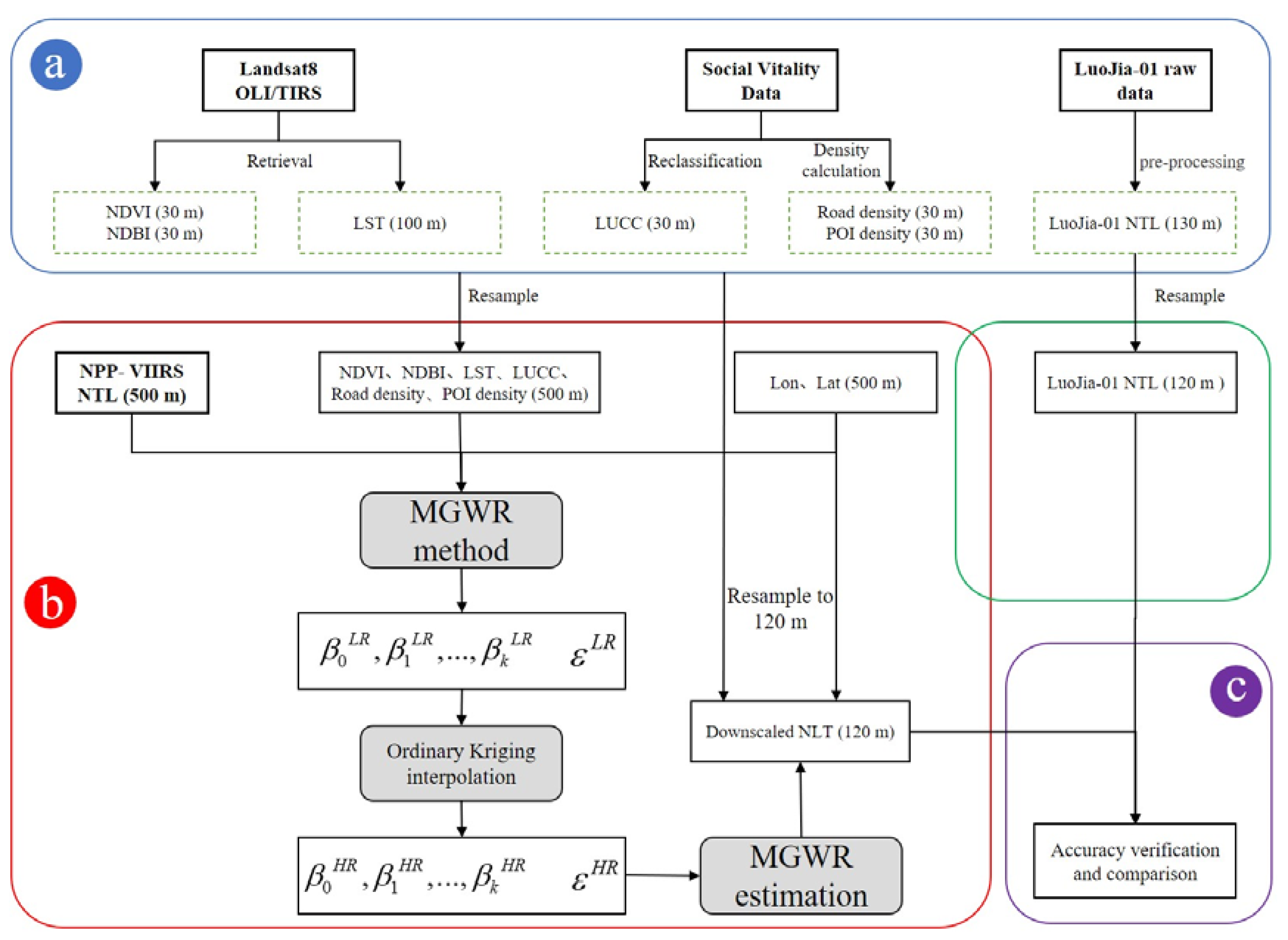
Figure 2. The proposed methodology for spatial downscaling of NTL data using MGWR.
Remotesensing 14 06400 g002

3.1. Processing Imagery

NDVI (30 m), NDBI (30 m), and LST (30 m) at a fine spatial resolution were calculated using Landsat 8 OLI/TIRS band data. The following formulas were used to compute the NDVI and NDBI [59].
The near-infrared reflectance (b5) to the red band (b4) reflectance ratio was used to determine the NDVI:
NDVI = ρ N I R ρ R ρ N I R + ρ R
The ratio of the reflectance in the red band (b6) to the near-infrared reflectance (b5) was used to calculate the NDBI:
NDBI = ρ S W I 1 ρ N I R ρ S W I 1 + ρ N I R
Surface temperature is a crucial indicator for keeping track of the ecological environment as it directly affects land, air moisture, and the atmosphere. The LST was calculated using the atmospheric correction approach [60,61]. The basic principle of the atmospheric correction method is to subtract the influence of the atmosphere on the surface thermal radiation from the total thermal radiation observed by the satellite sensor to obtain the surface thermal radiation intensity, which is then converted into the corresponding surface temperature. The thermal infrared radiance value received by the satellite sensor is composed of three parts: the upward radiance of the atmosphere I , the true radiance of the ground reaching the satellite sensor after passing through the atmosphere; after reaching the ground, the downward radiant energy of the atmosphere I reflected the energy [62].
LST = K 2 I n ( K 1 B ( T S ) + 1 ) 273
B ( T S ) = L I τ × ( 1 ε ) I ε × τ
where I , and I are the upward and downward radiance of the atmosphere, respectively; τ is the transmittance of the atmosphere in the thermal infrared band; and K 1 , K 2 are the calibration coefficients, which were obtained from the Atmospheric Correction Parameter Calculator (https://atmcorr.gsfc.nasa.gov, accessed on 10 June 2022) provided by the National Aeronautics and Space Administration (NASA). The imaging time, latitude, and longitude of the imaging center were input into the calculator to obtain I , I , τ , K 1 , and K 2 . In this study, K 1 = 774.89 W / ( m 2 sr μ m ) , and K 2 = 1321.08 K .
The NDVI threshold method proposed by Sobrino was used to calculate ε .
ε = 0.004 P V + 0.986 ,
where P V is the vegetation coverage, calculated using the following formula:
P V = NDVI NDVI S o i l NDVI V e g NDVI S o i l
Among them, NDVI is the normalized vegetation index; NDVI S o i l is the NDVI value of completely bare soil or the area with no vegetation cover; and NDVI V e g is the NDVI value for the pixel point completely covered by vegetation, i.e., the NDVI value of the pure vegetation pixel. Based on the empirical values, NDVI V e g = 0.70, and NDVI S o i l = 0.05, which implies that when the NDVI of a pixel is greater than 0.70, P V = 1; and when the NDVI is less than 0.05, P V = 0.
The POI and road data acquired for this investigation were vector data. Road and POI density were computed using ArcGIS 10.2 software and transformed into raster data to simplify the calculation.
To reduce data volume, the original LuoJia1-01 data was represented by DN. The calibration equation given by Zhang [18] between the actual radiance and the DN value is as follows:
L = D N 3 10 10 ,
where L is the adjusted absolute radiance value in W / ( m 2 s r μ m ) . However, the radiance value, as reported in the NPP-VIIRS data, is the spectral response function weighed value for the spectral range of 0.5–0.9 µm and is in the unit of n W / ( c m 2 s r ) . To ensure the comparability of the NTL data from these two sensors, the radiation units of LuoJia1-01 were converted into the radiation units of NPP-VIIRS using the following equation [63]:
L = Δ λ L 10 5 ,
where Δ λ (520 nm) is the bandwidth of LuoJia1-01 and L is the converted radiance.
The WGS 84 UTM Zone 50N coordinate system was used to project all the data in this study, ensuring that the geographic data coincided geographically without any offset.

3.2. MGWR

Local regression models such as GWR, Geographically and Temporally Weighted Regression (GTWR), and Geographically Weighted Auto Regressive (GWAR) are based on a constant bandwidth setting, limiting the bandwidth variation for each covariate, thereby excluding their scaling differences. Given the limitations of traditional GWR, Fotheringham [40] proposed the MGWR and made improvements based on the statistical inference of local parameters as proposed by Yu [48]. MGWR may discriminate between local, regional, and global scale processes for numerous covariates by doing away with the single bandwidth assumption of variables. Additionally, it generates processes similar to real estate space [48]. The MGWR calculation formula is presented as follows:
y i = j = 1 k β b w j ( u i , v i ) x i j + ε ,
where y i is the response variable; x i j is a covariate; β b w j represents the j th local regression coefficient with bandwidth b w ; ( u i , v i ) represents the spatial location of the sample point; and ε is the model regression residual. Unlike conventional GWR, each regression line in MGWR is created using a local regression process and has a separate bandwidth setting. Contrastingly, the bandwidth configurations of all covariates in conventional GWR are identical. A generalized additive model, which can be written as follows, may be used to describe the overall fit of the MGWR:
y = j = 1 k f i + ε , f j = β b w j x j ,
where y is the response variable; x j is the j th covariate; β b w j represents the j th local regression coefficient with bandwidth b w ; and ε is the regression residual of the model.
The backward-fitting approach is primarily used to fit each smooth term in the model. The final MGWR simulation is accomplished by successively determining the ideal bandwidth for various variables, using the conventional GWR estimate as the initial configuration. The parameter estimation is continuously updated until the coefficients iteratively converge. In the iterative convergence process for the coefficients, the larger the number of covariates, the more iterations are required for the model to converge [41]. The higher the degree of multicollinearity between the covariates, the more iterations are required before the model converges. The convergence phase of a local regression process will require more iterations than a regional or global regression process. In this study, we used the MGWR site package of the Python environment to construct the MGWR relationship model between NPP-VIIRS NTL intensity and NDVI, NDBI, LUCC, road density, POI density, LST, latitude, and longitude. When constructing a GWR model, the choice of spatially weighted kernel function and the bandwidth is highly important, and an inappropriate kernel function will lead to a poor data fit. If the bandwidth is too small, the data will be too noisy; if the bandwidth is too large, more details will be sacrificed. In the process of MGWR model building, the quadratic kernel function is most used, and Akaike Information Criteria (AICc) are used for the selection criteria of the kernel function and bandwidth. Simultaneously, the golden section algorithm searches for the optimal bandwidth [64].

3.3. Downscaling

To increase the spatial resolution of the NPP-VIIRS NTL images, we downscaled them from 500 m to 120 m. The downscaling process is based on many auxiliary variable sources, including latitude and longitude data, road density, POI density, NDVI, NDBI, LUCC, and LST. These auxiliary variables were chosen by considering their correlation with NTL intensity and data accessibility. We further describe the correlation between each variable and NTL intensity in Table 3. These data can be used to downscale NTL images because each of them can reflect some of the socioeconomic or physical geographic information associated with NTL intensity. Given that the influence factors of NTL intensity are complex, it is difficult to explain using a single data type in practice. Studies showed that the quantitative relationship between NTL intensity and surface physical parameters shows little change at different spatial resolutions [29]. According to the principle of the ‘constant relational scale’, NTL spatial downscaling can be performed by first building image pairs between high and low spatial resolution images and then applying it to high spatial resolution and performing residual correction.
NTL possesses non-stationary relationships with environmental factors at different scales. The multiscale and spatial non-stationary interactions may be modeled using MGWR, and the optimal scale at which these processes operate can also be determined. Therefore, spatial downscaling of NPP-VIIRS NTL data was performed using MGWR in this study. The specific technical route is shown in Figure 2. We used 500 m spatial resolution data as training data to construct the MGWR model and 120 m spatial resolution data as test data to obtain the downscaled NTL results. The LuoJia1-01 NTL data were used as the actual NTL data to test the model accuracy and were not involved in the modeling. The detailed downscaling conversion process is as follows:
(1)
NDVI, NDBI, road density, POI density, LUCC, LST, latitude, and longitude information were extracted at a 30-m resolution based on the Landsat 8 satellite imagery and other auxiliary data. The bilinear interpolation method was used to aggregate the spatial resolution to 120 m and 500 m;
(2)
MGWR was used to construct the multiscale spatial non-stationary functional relationship between NPP-VIIRS and NDVI, NDBI, road density, POI density, LUCC, LST, and the latitude and longitude information at a 500 m resolution:
N 500 = f ( NDVI 500 , NDBI 500 , Road 500 , POI 500 , LUCC 500 , LST 500 , Lon 500 , Lat 500 ) ,
where N 500 is the NTL intensity estimated by the scale conversion function at the 500 m resolution scale; f ( ) is the MGWR that converts the auxiliary variables to simulate NTL; NDVI 500 , NDBI 500 , Road 500 , POI 500 , LUCC 500 , LST 500 , Lon 500 , and Lat 500 are auxiliary variables at 500 m resolution;
(3)
Influenced by other surface physical parameters such as soil moisture, it is difficult for the selected auxiliary variables to fully reflect the spatial heterogeneity of the NTL, which is manifested as NTL residual information at low spatial resolution scales [65], which is:
Δ N S = N S N S ¯ ,
where Δ N S is the NTL transformation residual at 500 m resolution; N S and N S ¯ are the NTL data at a 500-m resolution and the NTL data estimated by the MGWR, respectively. Assuming that the residuals are uniformly spatially distributed, we further interpolated the transformed residuals to a resolution of 120 m using ordinary kriging interpolation [66]. Ordinary kriging interpolation is a linear estimation of regionalized variables. Assuming that the data are normally distributed, the expected value of the regionalized variable is considered to be unknown, and the approximate value of the to-be-interpolated point is obtained by determining the weight of the sampling points around the to-be-interpolated point.
(4)
According to the ‘constant relational scale’ principle, f ( ) established at low spatial resolution scales is still applicable at other spatial resolutions. Combined with the transformed residuals after spatial interpolation, the NTL data downscaled to a 120-m resolution is expressed as:
N 120 = f ( NDVI 120 , NDBI 120 , Road 120 , POI 120 , LUCC 120 , LST 120 , Lon 120 , Lat 120 ) + Δ N S ,
where N 120 is the downscaled NTL data at a resolution of 120 m; f ( ) is the MGWR function that converts the auxiliary variables to NTL data; NDVI 120 , NDBI 120 , Road 120 , POI 120 , LUCC 120 , LST 120 , Lon 120 , and Lat 120 are the 120 m resolution auxiliary variables after spatial aggregation; and Δ N S is the 120 m resolution conversion residual after spatial interpolation.

3.4. Validation and Method Comparison

We considered the LuoJia1-01 NTL remote sensing image data as the actual NTL data and evaluated the performance of the downscaling model by comparing the downscaled NTL data with the actual NTL data. The accuracy of downscaled NTL is mainly quantitatively evaluated using the root mean square error (RMSE) and the correlation coefficient (R2). RMSE and R2 are quantitative indicators for evaluating the accuracy of the data, which can be used to measure the degree of data deviation and the goodness of linear fit between the predicted and true values. Among them, the smaller the RMSE values, the smaller the error of the downscaled NTL data. The larger the R2 value, the higher the accuracy of the downscaled NTL data. The calculation formulas of RMSE and R2 are expressed as follows:
R M S E = 1 n i = 1 n ( N S oi N S ei ) 2 ,
R 2 = i = 1 n ( N ¯ i μ N ) 2 i = 1 n ( N i μ N ) 2 ,
where N S oi is the real NTL value of the i th pixel; N S ei is the NTL value simulated by the downscaling method corresponding to the i th pixel; RMSE is the root mean square error; n is the number of image elements involved in the evaluation. R2 is the coefficient of determination; N i and N ¯ i represent the LuoJia1-01 NTL image value and the downscaled NTL remote sensing image value, respectively; and μ N represents the average value for the LuoJia1-01 NTL value.
To further compare the advantages and disadvantages of MGWR, GWR and RF were used to perform spatial downscaling analysis on the NPP-VIIRS NTL data based on the same remote sensing data source and the downscaling process. The results were compared to that of the LuoJia1-01 NTL data as well. The GWR and RF based downscaling was implemented using the same auxiliary variables used for MGWR and are representative in characterizing the relationships between variables, spatial non-smoothness, and non-linear relationships.
The GWR regression function can be expressed as [67]:
y i = β 0 ( u i , v i ) + j = 1 k β j ( u i , v i ) x i j + ε i ,
where y i and x i j are the dependent and j th independent variables at location i , respectively. β ( u i , v i ) is the j th regression coefficient at location i , and ε i is the stochastic error term. The coefficient β is a function of the geographical location and can be estimated from weighted least-squares values.
RF is an ensemble learning technique consisting of the aggregation of a large number of decision trees, resulting in a reduction of variance compared to those of the single decision trees. The RF regression function can be expressed as [67]:
y i = f ( NDVI , NDBI , Road , POI , LUCC , LST , Lon , La t ) .
Assuming that the relationship acquired via RF remained constant between coarse and high resolutions, the RF-based downscaling results at a resolution of 120 m were calculated and compared to those of LuoJia1-01 NTL values.

4. Results

4.1. Correlation Analysis of the Variables

Table 3 lists the Pearson correlation coefficient (PCC) values between the NPP-VIIRS NTL data and auxiliary variables. The PCC ranged from −0.27 to 0.29, and the absolute mean was 0.22. This indicates that the NTL value was not determined by a single variable, whose value is affected simultaneously by multiple variables. Among these variables, the PCC of the POI and road densities was high and indicated a positive effect, suggesting that NTLs are closely related to human activities. The NDVI and NTL values are negatively correlated because areas with high NDVI are covered with a large amount of vegetation, which hinders the rise of NTL or reduced surface reflectivity. Simultaneously, LST was positively correlated with NTL intensity because the LST reflects the urban heat island environment, which is highly correlated with the expansion of buildings and impervious surfaces during urbanization [22].
Table 3 also lists the statistics for each regression coefficient of the MGWR model. From the absolute value of the regression coefficient of each auxiliary variable, the influence intensity of the POI density was the largest among all the variables, which proves that human activities play a key role in the distribution pattern of NTLs. The influence intensity of NDVI and the road density was high, which largely determines the spatial differentiation of NTL data, and the influence intensity for NDBI, LUCC, and LST was generally weak.

4.2. Accuracy Evaluation of the MGWR Model

Figure 3 displays the scatter plot between the downscaled NTL data and LuoJia1-01 NTL data. The results showed that MGWR had the highest precision, followed by GWR, and RF had the lowest precision. The coefficient of determination (R2) for the MGWR model was 0.9141 (the slope is close to 1), and RMSE was 16.87 nW / ( cm 2 sr ) at the significant level. The GWR had a relatively high R2 of 0.9085, but the RMSE was 1.7 times higher than the MGWR (Figure 3b). The overall accuracy of the RF is low, but the RMSE value was only slightly lower than that of the MGWR (Figure 3c). These results showed that the MGWR is more robust than other algorithms under the same auxiliary variables and exhibits the best downscaling accuracy.
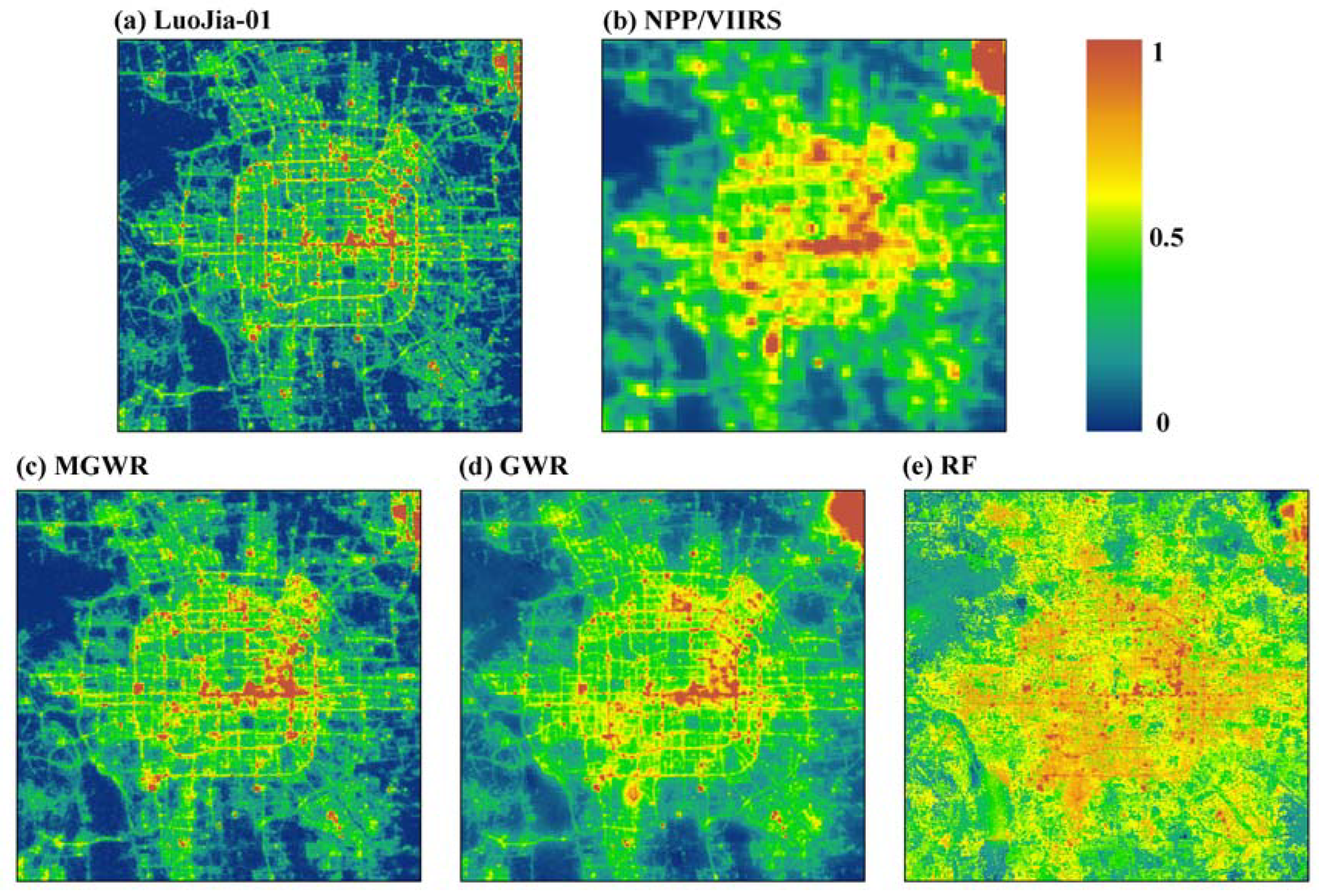
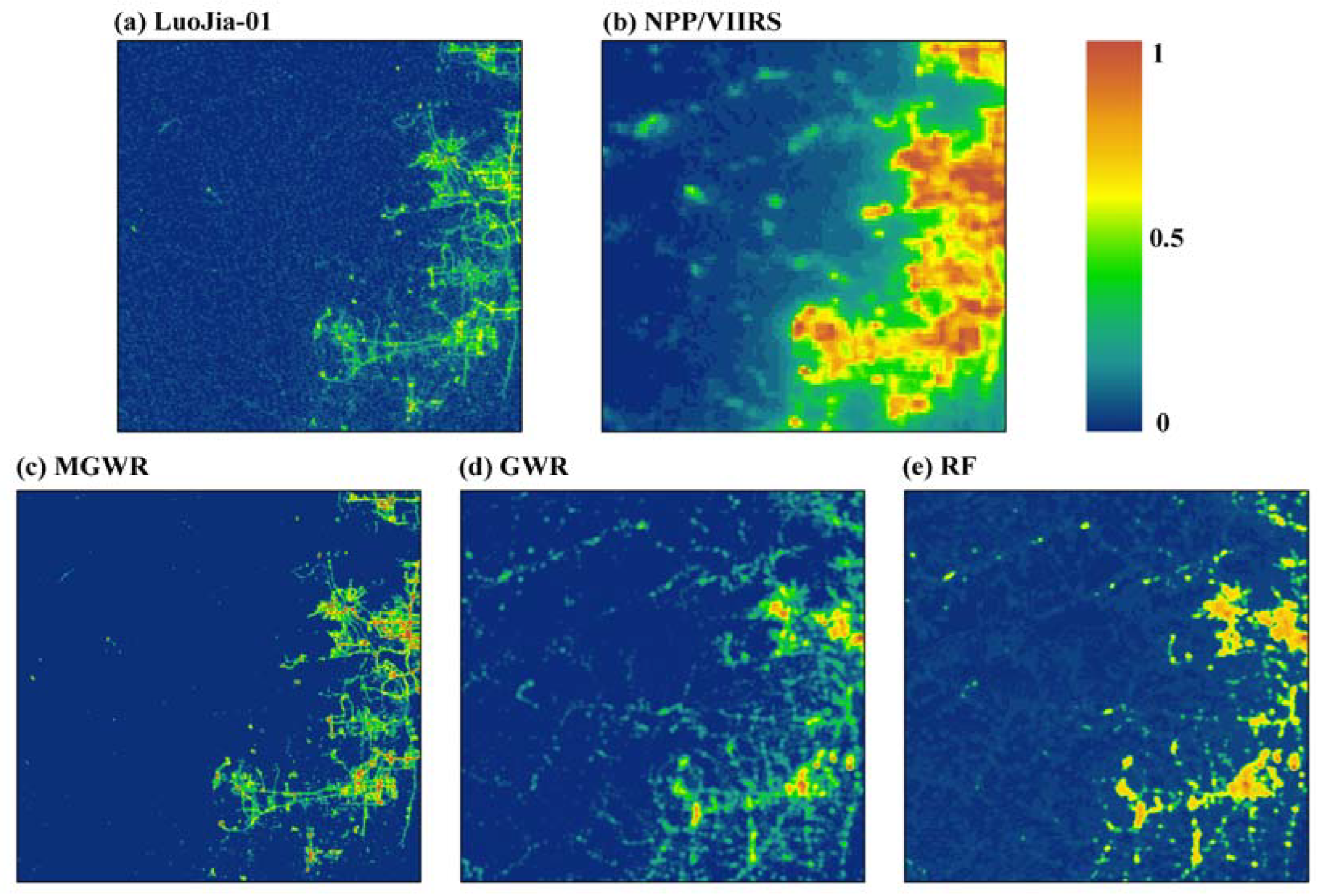
Figure 4 shows the original NPP-VIIRS NTL data, the downscaled NTL data predicted by the three downscaling methods (MGWR, GWR, and RF), and the LuoJia1-01 NTL data used for comparison. It shows that the spatial distribution of the NTL data downscaled using the three methods was consistent with that of the original data and had the same distribution as LuoJia1-01. Specifically, the MGWR algorithm could extract more NTL spatial texture information, revealing the differences in NTL distribution within similar ground cover types. Additionally, the GWR algorithm captured most of the NTL data in the original image, which objectively reflects the actual distribution of lights at night. However, when the light values increased, the image elements lost many component features within some regions, resulting in large errors and unclear textures. RF is not sensitive to spatial location and cannot explain the spatial heterogeneity of complex landscapes. Hence it can only roughly reveal the spatial distribution of NTL. The error of downscaling results was the largest and generally high.
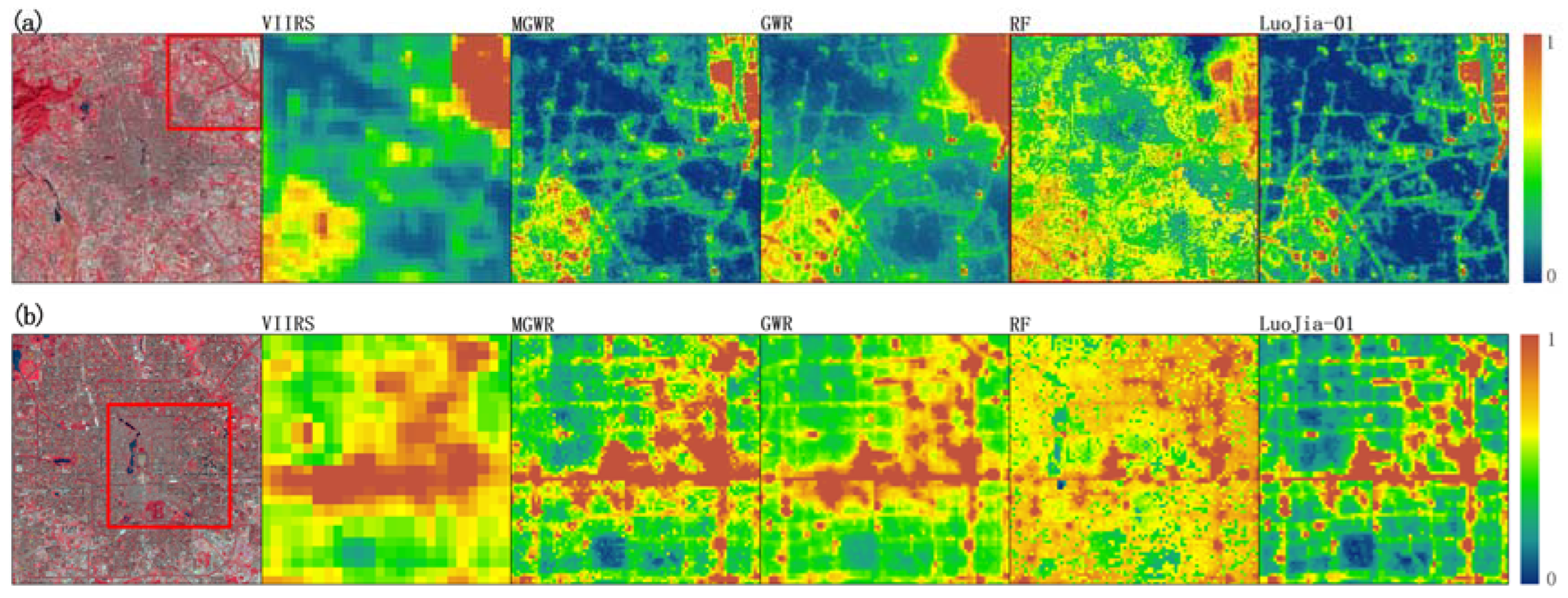
To compare the performance of different downscaling methods more clearly, we further selected two representative areas for more detailed visual analysis (Figure 5). In both Beijing Capital International Airport (Figure 5a) and part of Central Beijing (Figure 5b), the three downscaling methods considerably enhanced the spatial texture of the original NTL data. However, there were still substantial differences in the details. MGWR depicted the interior spatial textures of the suburbs and the central city in more detail. The spatial differences of NTL data were also highly consistent with those of LuoJia1-01. We found that MGWR-downscaled NTL data were more accurate than those obtained using other methods in some areas with increased NTLs, such as airports. Compared with MGWR, GWR showed similar downscaled results, although it smoothened out the detailed variation in areas with increased high NTLs and clearly overestimated the NTL levels around the airport. In areas with relatively large differences in surface coverage, such as the airport, RF outperformed GWR. However, RF had the worst overall downscaled performance, revealing only the approximate distribution of surface coverage, with abrupt transitional changes between NTLs. Additionally, a problem of large-scale overestimation in the central city existed. For suburban airports and central urban areas with large nighttime lighting changes, MGWR can reveal more NTL radiation features, reflecting the NTL differentiation caused by land cover changes and population activities and ensuring the downscaling of NTL data.

5. Discussion

5.1. Effect of MGWR Bandwidth on NTL Data Downscaling in the Study Area

The reason MGWR outperforms GWR is that by setting different bandwidths for each auxiliary variable, MGWR allows processes to operate at different spatial scales based on the characteristics of different variables. However, GWR assumes that all modeled processes operate at the same spatial scale. Here we further confirmed that different variables have different action scales by calculating the bandwidths of variables.
We employed the commonly used quadratic kernel function, AICc, and the golden ratio to search for the optimal bandwidth. The optimal bandwidth can be used as the basis for determining whether the influence of the corresponding variable of the independent variable is at the global or local scale. Table 4 shows the difference in the action scale for each auxiliary variable when it affects the spatial pattern differentiation of NTLs. The larger the action scale, the greater the global influence of the corresponding variable of the auxiliary variables, with contrasting local influence.
Table 4 shows that the MGWR can be used to directly reflect the difference in the action scales of different covariates, but classical GWR can only show the average value of the action scales for each covariate. Through the estimation of the MGWR, we found that the action scales for different factors were quite different. The bandwidths of 43 for NDVI, POI, and Intercept indicate that the NTL intensity is sensitive to the response of these auxiliary variables. Simultaneously, road density and LST are also sensitive (<50). This phenomenon reflects that the NTL data of the main urban area of Beijing had high spatial variation from one area to another. Contrastingly, the effects of NDBI and LUCC on NTL were relatively stable, with effective scales of 707 and 558, respectively. This suggests that building and land use types had prominent effects at any scale. The density of buildings and the land use type determine the number of lights at night. The synergy of land cover and urban construction affected the spatially differentiated characteristics of NTLs, showing a relatively small scale of influence. The NDBI and LUCC encompass the global scale for NTL images, which shows it is correct for many city boundary extraction algorithms to use NTL data to increase their accuracy.
Conclusively, compared with the traditional GWR, MGWR can better reveal the effects of different auxiliary variables on the spatial distribution of NTL and the scale differences of spatial heterogeneity. Therefore, it is of practical importance to use MGWR to explore the spatial downscaling of NPP-VIIRS NTL.

5.2. Rationalization of Downscaling Based on MGWR

The quantitative relationship between NTL and impact factor varies less at different spatial resolution scales, i.e., the relationship model between NTL and impact factor at low spatial resolution is still applicable at a high spatial resolution [68]. In this study, spatial downscaling of NPP-VIIRS NTL data was performed using MGWR, which is a statistical regression algorithm based on the ‘constant relational scale’ principle. However, the ‘constant relational scale’ principle has only been proven to be successfully applied to topographically homogeneous surfaces and areas with homogeneous land cover and has certain conditions and limitations of applicability for heterogeneous landscape surfaces [65,69]. To verify if it is reasonable to use this principle in this study area, bilinear interpolation was used to resample LuoJia1-01 NTL data and POI density data to 600, 480, 360, 240, and 120 m, and then calculated the correlation between LuoJia1-01 NTL brightness and POI density at different resolutions [49,68].
As shown in Table 5, the differences in the coefficients and intercepts of the linear relationship between NTL intensity and POI density increased as the differences in image resolution increased. Particularly, when the spatial resolution was between 240 m and 480 m, the relationship between NTL intensity and POI density did not change much, and the principle of ‘constant relational scale’ can be satisfied. Pixel points were selected in a part of Central Beijing (Figure 5b) of the study area for analysis. Table 5 shows that the linear relationship between NTL intensity and POI density differed at different resolution scales. Generally, the relationship varied less in the central urban area than in the whole study area. This confirms that the ‘constant relational scale’ principle has good application performance in areas with uniform NTL.
The principle of ‘constant relational scale’ was not feasible in the non-uniform areas of the surface, and the quantitative relationship between NTL intensity and POI density at 120 m and 600 m resolution scales was inconsistent. However, according to our results, the impact of surface heterogeneity was not significant. The statistical MGWR regression model proposed in this study based on the principle of ‘constant relational scale’ still greatly increased the downscaling accuracy of the NPP-VIIRS NTL data in the study area.

5.3. Application of the MGWR Model in Other Cases

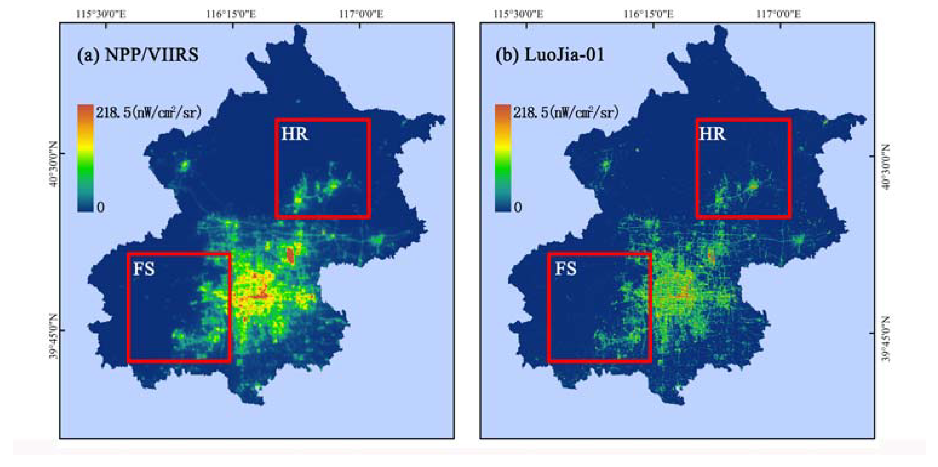
To prove the feasibility of the MGWR model in downscaling NTL data, we applied it elsewhere in Beijing. The two cases we used for validation, Huairou (HR) and Fangshan (FS), are shown in Figure 6. They are both located at the urban-rural border of Beijing and have different spatial distribution characteristics from the NTL in the study area (Figure 1).
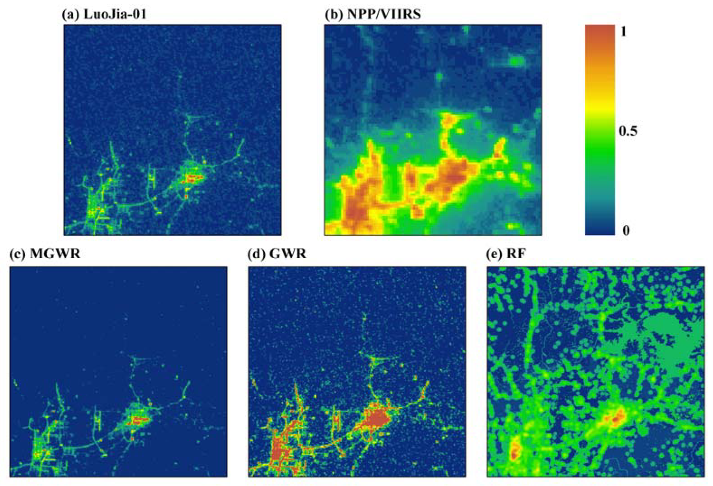
Figure 7 and Figure 8 show the downscaled NTL data for the validation regions of HR and FS, respectively. It shows that the spatial distribution of the downscaled NTL data completed by the three methods was consistent with that of the original data and had the same distribution as LuoJia1-01. Here we unexpectedly found that MGWR was not only more accurate overall than those of the other two methods but was also able to capture small areas of bright spots in dark areas. Otherwise, the results of the three downscaling methods showed characteristics consistent with the study area in the validation areas. Therefore, the MGWR model has a degree of applicability in different regions.

5.4. Strengths and Limitations

The spatial resolution of the NPP-VIIRS NTL data was refined in this study, enabling further applications requiring higher spatial resolution. The strengths of the study are as follows:
(1)
The multivariate-based MGWR method better described the spatial variation of NTL data than the GWR and RF methods. The downscaled NTL images showed higher spatial resolution than the original NTL data in terms of more detailed information and sharper boundaries;
(2)
Due to the pronounced spatial heterogeneity scale differences of various influencing factors on the distribution of NTLs, it was difficult for global statistical regression and classical GWR models to reveal the spatial heterogeneity scale effects between the NTLs and auxiliary variables. The proposed MGWR downscaling model improved the classical GWR method by allowing individual auxiliary variables to have different bandwidth settings according to the range of influence scales. Therefore, it can provide a more realistic and effective description of the spatial process and better explain the effects of different auxiliary variables on the spatial variation of NTLs;
(3)
The MGWR proposed in this study mainly uses eight auxiliary variables: NDVI, NDBI, road density, POI density, LUCC, LST, latitude, and longitude, which strongly correlated with the NTL data. For the spatial downscaling of the NTLs, the construction of the relational model and the selection of the auxiliary variables were directly related to whether accurate and reliable high-spatial-resolution NTL data could be obtained. By capturing the different auxiliary variables of various auxiliary variables on the NTL distribution, MGWR avoids the introduction of excessive noise and bias in constructing the NTL conversion function and provides technical support for the accurate realization of downscaling NTL data.
Our study is meaningful for increasing the spatial resolution of NPP-VIIRS NTL data, although some shortcomings and scope for future work still exist.
(1)
When using remote sensing images as auxiliary data to downscale the NPP-VIIRS NTL data, the time difference between the different satellite transits will affect the downscaling accuracy. In this study, we removed the temporal error by averaging the multi-temporal Landsat 8 OLI and NPP-VIIRS NTL sensor data, although some uncertainty when predicting high-resolution NTL data may exist. When there is no auxiliary information, such as in Landsat satellite data, to perform downscaling in the study area, spatiotemporal fusion or reconstruction of corresponding auxiliary data is necessary for the spatial downscaling of NPP-VIIRS NTL data [70]. This condition increases the difficulty of the operation and may introduce some errors in data fusion or reconstruction. In the future, we will consider calibrating MGWR with more models.
(2)
Based on statistical regression, the downscaling process is not only considerably affected by the regression model but was also closely related to the land cover type and the state of the atmospheric environment. Therefore, to develop an NTL data downscaling model with greater applicability, selecting more study areas and periods is necessary for future testing.

6. Conclusions

NPP-VIIRS NTL data are considered the most suitable data for assessing demographic and socioeconomic characteristics, although their full potential is limited by their coarse spatial resolution. According to the principle of ‘constant relational scale’, we proposed a downscaling framework based on the MGWR. To our best knowledge, it is the first to propose a framework to downscale NTL data based on auxiliary variables and the GWR method to a finer resolution of 120 m. We compared the downscaled image with the LuoJia1-01 image to validate the downscaling accuracy. To evaluate the goodness of fit, MGWR was compared with two representative methods, GWR and RF.
The main results generated were as follows: (1) Among all the auxiliary variables, the POI density attained the highest correlation with the NTL value, with the highest PCC value of 0.29. (2) The results of downscaling via MGWR exhibited higher R2 (0.91 vs. 0.90 vs. 0.87) and lower RMSE (29.00 vs. 17.57 vs. 16.87 nW/cm2/sr) compared with the results of GWR and RF algorithms, indicating enhancement of the spatial resolution of the data after downscaling. (3) MGWR captured the effects of multiple auxiliary variables on NTL distribution by setting different bandwidths and avoided introducing excessive noise and bias in the process of constructing NTL transformation functions, which provides technical support for obtaining accurate downscaled NTL data. Therefore, the NTL spatial downscaling method based on MGWR used in this study can increase the texture information of low-spatial-resolution NTL data and ensure the accuracy and spatial consistency of the downscaled NTL data. For research fields involving the estimation of population distribution, social economy, and urban development and planning, this method can provide reliable high-spatial-resolution NTL remote sensing datasets.

Author Contributions

Conceptualization, S.L. and X.Z.; methodology, S.L.; validation, S.L. and L.C.; investigation, F.Z.; resources, F.Z.; data curation, X.Z.; writing—original draft preparation, S.L.; writing—review and editing, X.Z.; visualization, A.Q. and S.Z.; supervision, A.Q., S.C. and J.H.; project administration, L.C. and J.H.; funding acquisition, A.Q. and F.Z. All authors have read and agreed to the published version of the manuscript.

Funding

This research was funded by the National Key R&D Program of China [grant numbers 2019YFB2102503, 2019YFB2102500]; National Natural Science Foundation of China [No. 42201434]; LZJTU [grant numbers 201806]; Chinese Academy of Surveying and Mapping Basic Research Fund Program [grant number AR2111].

Conflicts of Interest

The authors declare no conflict of interest.

References

  1. Sutton, P.; Roberts, D.; Elvidge, C.; Baugh, K. Census from Heaven: An estimate of the global human population using night-time satellite imagery. Int. J. Remote Sens. 2001, 22, 3061–3076. [Google Scholar] [CrossRef]
  2. Xu, H.; Yang, H.; Li, X.; Jin, H.; Li, D. Multi-Scale Measurement of Regional Inequality in Mainland China during 2005–2010 Using DMSP/OLS Night Light Imagery and Population Density Grid Data. Sustainability 2015, 7, 13469–13499. [Google Scholar] [CrossRef] [Green Version]
  3. Wang, C.; Chen, Z.; Yang, C.; Li, Q.; Wu, Q.; Wu, J.; Zhang, G.; Yu, B. Analyzing parcel-level relationships between Luojia 1-01 nighttime light intensity and artificial surface features across Shanghai, China: A comparison with NPP-VIIRS data. Int. J. Appl. Earth Obs. Geoinf. 2020, 85, 101989. [Google Scholar] [CrossRef]
  4. Yu, B.; Lian, T.; Huang, Y.; Yao, S.; Ye, X.; Chen, Z.; Yang, C.; Wu, J. Integration of nighttime light remote sensing images and taxi GPS tracking data for population surface enhancement. Int. J. Geogr. Inf. Sci. 2019, 33, 687–706. [Google Scholar] [CrossRef]
  5. Shi, K.; Huang, C.; Yu, B.; Yin, B.; Huang, Y.; Wu, J. Evaluation of NPP-VIIRS night-time light composite data for extracting built-up urban areas. Remote Sens. Lett. 2014, 5, 358–366. [Google Scholar] [CrossRef]
  6. Chen, Z.; Yu, B.; Zhou, Y.; Liu, H.; Yang, C.; Shi, K.; Wu, J. Mapping Global Urban Areas From 2000 to 2012 Using Time-Series Nighttime Light Data and MODIS Products. IEEE J. Sel. Top. Appl. Earth Obs. Remote Sens. 2019, 12, 1143–1153. [Google Scholar] [CrossRef]
  7. Li, Y.; Song, Z.; Wu, B.; Yu, B.; Wu, Q.; Hong, Y.; Liu, S.; Wu, J. Evaluating the Ability of NOAA-20 Monthly Composite Data for Socioeconomic Indicators Estimation and Urban Area Extraction. IEEE J. Sel. Top. Appl. Earth Obs. Remote Sens. 2022, 15, 1837–1845. [Google Scholar] [CrossRef]
  8. Yu, B.; Tang, M.; Wu, Q.; Yang, C.; Deng, S.; Shi, K.; Peng, C.; Wu, J.; Chen, Z. Urban Built-Up Area Extraction From Log- Transformed NPP-VIIRS Nighttime Light Composite Data. IEEE Geosci. Remote Sens. Lett. 2018, 15, 1279–1283. [Google Scholar] [CrossRef]
  9. Chen, Z.; Yu, B.; Hu, Y.; Huang, C.; Shi, K.; Wu, J. Estimating House Vacancy Rate in Metropolitan Areas Using NPP-VIIRS Nighttime Light Composite Data. IEEE J. Sel. Top. Appl. Earth Obs. Remote Sens. 2015, 8, 2188–2197. [Google Scholar] [CrossRef]
  10. Lu, H.; Zhang, C.; Liu, G.; Ye, X.; Miao, C. Mapping China’s Ghost Cities through the Combination of Nighttime Satellite Data and Daytime Satellite Data. Remote Sens. 2018, 10, 1037. [Google Scholar] [CrossRef]
  11. Chen, Z.; Yu, B.; Song, W.; Liu, H.; Wu, Q.; Shi, K.; Wu, J. A New Approach for Detecting Urban Centers and Their Spatial Structure with Nighttime Light Remote Sensing. IEEE Trans. Geosci. Remote Sens. 2017, 55, 6305–6319. [Google Scholar] [CrossRef]
  12. Wu, B.; Yu, B.; Yao, S.; Wu, Q.; Chen, Z.; Wu, J. A surface network based method for studying urban hierarchies by night time light remote sensing data. Int. J. Geogr. Inf. Sci. 2019, 33, 1377–1398. [Google Scholar] [CrossRef]
  13. Cheng, B.; Chen, Z.; Yu, B.; Li, Q.; Wang, C.; Li, B.; Wu, B.; Li, Y.; Wu, J. Automated Extraction of Street Lights from JL1-3B Nighttime Light Data and Assessment of Their Solar Energy Potential. IEEE J. Sel. Top. Appl. Earth Obs. Remote Sens. 2020, 13, 675–684. [Google Scholar] [CrossRef]
  14. Ou, J.; Liu, X.; Liu, P.; Liu, X. Evaluation of Luojia 1-01 nighttime light imagery for impervious surface detection: A comparison with NPP-VIIRS nighttime light data. Int. J. Appl. Earth Obs. Geoinf. 2019, 81, 1–12. [Google Scholar] [CrossRef]
  15. Guo, W.; Zhang, Y.; Gao, L. Using VIIRS-DNB and landsat data for impervious surface area mapping in an arid/semiarid region. Remote Sens. Lett. 2018, 9, 587–596. [Google Scholar] [CrossRef]
  16. Guo, W.; Lu, D.; Wu, Y.; Zhang, J. Mapping Impervious Surface Distribution with Integration of Snnp Viirs-NDB Modis Ndvi Data. Remote Sens. 2015, 7, 12459–12477. [Google Scholar] [CrossRef] [Green Version]
  17. Baugh, K.; Hsu, F.-C.; Elvidge, C.D.; Zhizhin, M. Nighttime Lights Compositing Using the VIIRS Day-Night Band: Preliminary Results. Proc. Asia-Pac. Adv. Netw. 2013, 35, 70. [Google Scholar] [CrossRef] [Green Version]
  18. Zhang, G.; Li, L.; Jiang, Y.; Shen, X.; Li, D. On-orbit relative radiometric calibration of the night-time sensor of the luojia1-01 satellite. Sensors 2018, 18, 4225. [Google Scholar] [CrossRef] [Green Version]
  19. Zheng, Q.; Weng, Q.; Huang, L.; Wang, K.; Deng, J.; Jiang, R.; Ye, Z.; Gan, M. A new source of multi-spectral high spatial resolution night-time light imagery—JL1-3B. Remote Sens. Environ. 2018, 215, 300–312. [Google Scholar] [CrossRef]
  20. Huang, B.; Zhao, Y. Resrarch Status and Prospect of Spatio temporal Fusion of Multi-source Satellite Remote Sensing Imagery. Acta Geod. Et Cartogr. Sin. 2017, 46, 1492–1499. [Google Scholar] [CrossRef]
  21. Luo, X.; Chen, Y.; Wang, Z.; Li, H.; Peng, Y. Spatial down-scaling of land surface temperature based on MODIS data. Chin. J. Ecol. 2016, 35, 3443–3450. [Google Scholar] [CrossRef]
  22. Wang, Z.; Qin, Q.; Sun, Y.; Zhang, T.; Ren, H. Downscaling remotely sensed land surface temperature with the BP neural network. Remote Sens. Technol. Appl. 2018, 33, 793–802. [Google Scholar] [CrossRef]
  23. Gao, F.; Masek, J.; Schwaller, M.; Hall, F. On the blending of the Landsat and MODIS surface reflectance: Predicting daily Landsat surface reflectance. IEEE Trans. Geosci. Remote Sens. 2006, 44, 2207–2218. [Google Scholar] [CrossRef]
  24. Zhang, B.; Zhang, L.; Xie, D.; Yin, X.; Liu, C.; Liu, G. Application of synthetic NDVI time series blended from Landsat and MODIS data for grassland biomass estimation. Remote Sens. 2016, 8, 10. [Google Scholar] [CrossRef] [Green Version]
  25. Hilker, T.; Wulder, M.A.; Coops, N.C.; Linke, J.; McDermid, G.; Masek, J.; Gao, F.; White, J.C. A new data fusion model for high spatial and temporal-resolution mapping of forest disturbance based on Landsat and MODIS. Remote Sens. Environ. 2009, 113, 1613–1627. [Google Scholar] [CrossRef]
  26. Liu, M.; Yang, W.; Zhu, X.L.; Chen, J.; Chen, X.H.; Yang, L.Q.; Helmer, E.H.; Huang, B.; Song, H. An Improved Flexible Spatiotemporal DAta Fusion (IFS-DAF) method for producing high spatiotemporal resolution normalized difference vegetation index time series. Remote Sens. Environ. 2019, 227, 74–89. [Google Scholar] [CrossRef]
  27. Shi, C.; Wang, X.; Zhang, M.; Liang, X.; Niu, L.; Han, H.; Zhu, X. A comprehensive and automated fusion method: The enhanced flexible spatiotemporal DAta fusion model for monitoring dynamic changes of land surface. Appl. Sci. 2019, 9, 3693. [Google Scholar] [CrossRef] [Green Version]
  28. Huang, B.; Jiang, X.L. An enhanced unmixing model for spatiotemporal image fusion. Natl. Remote Sens. Bull. 2021, 25, 241–250. [Google Scholar] [CrossRef]
  29. Zhan, W.; Chen, Y.; Zhou, J.; Li, J.; Liu, W.Y. Sharpening thermal imageries: A generalized theoretical framework from an assimilation perspective. IEEE Trans. Geosci. Remote Sens. 2011, 49, 773–789. [Google Scholar] [CrossRef]
  30. Dowman, I.R.; Hannes, I. Global geospatial data from Earth observation: Status and issues. Int. J. Digit. Earth 2016, 10, 328–341. [Google Scholar] [CrossRef]
  31. Guo, N.; Wang, X. Advances and developing opportunities in remote sensing of drought. J. Arid. Meteorol. 2015, 33, 1–18. [Google Scholar]
  32. Yang, Q.; Yuan, Q.; Li, T.; Yue, L. Mapping PM2.5 concentration at high resolution using a cascade random forest based downscaling model: Evaluation and application. J. Clean. Prod. 2020, 277, 123887. [Google Scholar] [CrossRef]
  33. Chen, C.; Zhao, S.; Duan, Z.; Qin, Z. An Improved Spatial Downscaling Procedure for TRMM 3B43 Precipitation Product Using Geographically Weighted Regression. IEEE J. Sel. Top. Appl. Earth Obs. Remote Sens. 2015, 8, 4592–4604. [Google Scholar] [CrossRef]
  34. Kustas, W.P.; Norman, J.M.; Anderson, M.C.; French, A.N. Estimating subpixel surface temperatures and energy fluxes from thevegetation index–radiometric temperature relationship. Remote Sens. Environ. 2003, 85, 429–440. [Google Scholar] [CrossRef]
  35. Agam, N.; Kustas, W.P.; Anderson, M.C.; Li, F.Q.; Neale, C.M.U. A vegetation index based technique for spatial sharpening of thermal imagery. Remote Sens. Environ. 2007, 107, 545–558. [Google Scholar] [CrossRef]
  36. Dominguez, A.; Kleiss, L.J.; Luvall, J.C.; Rickman, D.L. High-resolution urban thermal sharpener (HUTS). Remote Sens. Environ. 2011, 115, 1772–1780. [Google Scholar] [CrossRef] [Green Version]
  37. Zhu, S.; Guan, H.; Millington, A.C.; Zhang, G. Disaggre-gation of land surface temperature over a heterogeneous urban and surrounding suburban area: A case study in Shanghai. Int. J. Remote Sens. 2013, 34, 1707–1723. [Google Scholar] [CrossRef]
  38. Chen, Z.; Yu, B.; Yang, C.; Zhou, Y.; Yao, S.; Qian, X.; Wang, C.; Wu, B.; Wu, J. An extended time series (2000–2018) of global NPP-VIIRS-like nighttime light data from a cross-sensor calibration. Earth Syst. Sci. Data 2021, 13, 889–906. [Google Scholar] [CrossRef]
  39. Ye, Y.; Huang, L.; Zheng, Q.; Liang, C.; Dong, B.; Deng, J.; Han, X. A feasible framework to downscale NPP-VIIRS nighttime light imagery using multi-source spatial variables and geographically weighted regression. Int. J. Appl. Earth Obs. Geoinf. 2021, 104, 102513. [Google Scholar] [CrossRef]
  40. Fotheringham, S.; Yang, W.; Kang, W. Multiscale geographically weighted regression (MGWR). Ann. Am. Assoc. Geogr. 2017, 107, 1247–1265. [Google Scholar] [CrossRef]
  41. Shen, T.Y.; Yu, H.C.; Zhou, L.; Gu, H.Y.; He, H.H. On hedonic price of second-hand houses in Beijing based on multi-scale geo-graphically weighted regression: Scale law of spatial heterogeneity. Econ. Geogr. 2020, 40, 75–83. [Google Scholar] [CrossRef]
  42. Levin, N.; Johansen, K.; Hacker, J.M.; Phinn, S. A new source for high spatial resolution night time images—The EROS-B commercial satellite. Remote Sens. Environ. 2014, 149, 1–12. [Google Scholar] [CrossRef]
  43. Scher, C.L.; Karimi, N.; Glasenhardt, M.C.; Tuffin, A.; Cannon, C.H.; Scharenbroch, B.C.; Hipp, A.L. Application of remote sensing technology to estimate productivity and assess phylogenetic heritability. Appl. Plant Sci. 2020, 8, e11401. [Google Scholar] [CrossRef] [PubMed]
  44. Davis, A.Y.; Jung, J.; Pijanowski, B.C.; Minor, E.S. Combined vegetation volume and “greenness” affect urban air temperature. Appl. Geogr. 2016, 71, 106–114. [Google Scholar] [CrossRef] [Green Version]
  45. Li, F.; Yan, Q.; Bian, Z.; Liu, B.; Wu, Z. A poi and lst adjusted ntl urban index for urban built-up area extraction. Sensors 2020, 20, 2918. [Google Scholar] [CrossRef]
  46. Zhao, N.; Cao, G.; Zhang, W.; Samson, E.L.; Chen, Y. Remote sensing and social sensing for socioeconomic systems: A comparison study between nighttime lights and location-based social media at the 500 m spatial resolution. Int. J. Appl. Earth Obs. Geoinf. 2020, 87, 102058. [Google Scholar] [CrossRef]
  47. Levin, N.; Duke, Y. High spatial resolution night-time light images for demographic and socio-economic studies. Remote Sens. Environ. 2012, 119, 1–10. [Google Scholar] [CrossRef]
  48. Yu, H.; Fotheringham, A.S.; Li, Z.; Oshan, T.; Kang, W.; Wolf, L. Inference in multiscale geographically weighted regression. Geogr. Anal. 2019, 52, 87–106. [Google Scholar] [CrossRef]
  49. Zhu, X.M.; Song, X.N.; Leng, P.; Hu, R.H. Spatial downscaling of land surface temperature with the multi-scale geographically weighted regression. Natl. Remote Sens. Bull. 2021, 25, 1749–1766. [Google Scholar] [CrossRef]
  50. Sun, Y.; Wang, S.; Wang, Y. Estimating local-scale urban heat island intensity using nighttime light satellite imageries. Sustain. Cities Soc. 2020, 57, 102125. [Google Scholar] [CrossRef]
  51. Li, H.; Zhang, H.; Wang, M. A Comparative Study of Population Spatialization Based on NPP/VIIRS and LJ1-01 Night Data: Taking Beijing for an Example. Remote Sens. Inf. 2021, 36, 90–97. [Google Scholar] [CrossRef]
  52. Xu, J.; Wang, J.; Xiong, N.; Chen, Y.; Sun, L.; Wang, Y.; An, L. Analysis of Ecological Blockage Pattern in Beijing Important Ecological Function Area, China. Remote Sens. 2022, 14, 1151. [Google Scholar] [CrossRef]
  53. Elvidge, C.D.; Zhizhin, M.; Ghosh, T.; Hsu, F.-C.; Taneja, J. Annual Time Series of Global VIIRS Nighttime Lights Derived from Monthly Averages: 2012 to 2019. Remote Sens. 2021, 13, 922. [Google Scholar] [CrossRef]
  54. Elvidge, C.; Baugh, K.; Zhizhin, M.; Hsu, F.-C. Why VIIRS data are superior to DMSP for mapping nighttime lights. Proc. Asia-Pac. Adv. Netw. 2013, 35, 62–69. [Google Scholar] [CrossRef] [Green Version]
  55. Wang, Z.; Román, M.O.; Kalb, V.L.; Miller, S.D.; Zhang, J.; Shrestha, R.M. Quantifying uncertainties in nighttime light retrievals from Suomi-NPP and NOAA-20 VIIRS Day/Night Band data. Remote Sens. Environ. 2021, 263, 112557. [Google Scholar] [CrossRef]
  56. Wang, L.; Fan, H.; Wang, Y. Improving population mapping using Luojia 1–01 nighttime light image and location-based social media data. Total Env. 2020, 730, 139–148. [Google Scholar] [CrossRef]
  57. Ye, Y.; Xue, X.; Huang, L.; Gan, M.; Tong, C.; Wang, K.E.; Deng, J. A new persective to map the supply and demand of artificial night light based on Loujia1- 01 and urban big data. Clean. Prod 2020, 276, 123–244. [Google Scholar] [CrossRef]
  58. Foga, S.; Scaramuzza, P.L.; Guo, S.; Zhu, Z.; Dilley, R.D.; Beckmann, T.; Schmidt, G.L.; Dwyer, J.L.; Joseph Hughes, M.; Laue, B. Cloud detection algorithm comparison and validation for operational Landsat data products. Remote Sens. Environ. 2017, 194, 379–390. [Google Scholar] [CrossRef] [Green Version]
  59. Gao, P.W.; Kasim, A.; Ruzi, T.; Zhao, M.C. Temporal and spatial analysis of ecological environment improvement in Hami City. Arid Zone Res. 2020, 37, 1057–1067. [Google Scholar]
  60. Singh, A.K.; Toshniwal, D. A Big Data Approach for Situation-Aware correction and estimation of NDVI, based on Landsat8 OLI/TIRS (Surface Reflectance) time series data. Jpn. Geosci. Union. 2017. Available online: https://ui.adsabs.harvard.edu/abs/2017AGUFM.A41H2392S (accessed on 10 August 2022).
  61. Vermote, E.; Justice, C.; Claverie, M.; Franch, B. Preliminary analysis of the performance of the Landsat 8/OLI land surface reflectance product. Remote Sens. Environ. 2016, 185, 46–56. [Google Scholar] [CrossRef]
  62. Qi, J.; Li, X. Research on Retrieval of Surface Temperature Based on Landsat8 Data Atmospheric Correction Method. In Proceedings of the JpGU-AGU Joint Meeting, Chiba, Japan, 20–25 May 2017. [Google Scholar]
  63. Li, X.; Zhao, L.; Li, D.; Xu, H. Mapping Urban Extent Using Luojia 1–01 Nighttime Light Imagery. Sensors 2018, 18, 3665. [Google Scholar] [CrossRef] [PubMed] [Green Version]
  64. Oshan, T.M.; Li, Z.; Kang, W.; Wolf, L.J.; Fotheringham, A.S. mgwr: A Python Implementation of Multiscale Geographically Weighted Regression for Investigating Process Spatial Heterogeneity and Scale. ISPRS Int. J. Geo-Inf. 2019, 8, 269. [Google Scholar] [CrossRef]
  65. Mukherjee, S.; Joshi, P.K.; Garg, R.D. A comparison of different regression models for downscaling Landsat and MODIS land surface temperature images over heterogeneous landscape. Adv. Space Res. 2014, 54, 655–669. [Google Scholar] [CrossRef]
  66. Li, Y.; Baorong, Z.; Xiaohong, X.; Zijun, L. Application of a semivariogram based on a deep neural network to Ordinary Kriging interpolation of elevation data. PLoS ONE 2022, 17, e0266942. [Google Scholar] [CrossRef] [PubMed]
  67. Guo, B.; Bian, Y.; Zhang, D.; Su, Y.; Wang, X.; Zhang, B.; Wang, Y.; Chen, Q.; Wu, Y.; Luo, P. Estimating Socio-Economic Parameters via Machine Learning Methods Using Luojia1-01 Nighttime Light Remotely Sensed Images at Multiple Scales of China in 2018. IEEE Access 2021, 9, 34352–34365. [Google Scholar] [CrossRef]
  68. Zhan, W.; Chen, Y.; Wang, J.; Zhou, J.; Quan, J.; Liu, W.; Li, J. Downscaling land surface temperatures with multi-spectral and multi-resolution images. Int. J. Appl. Earth Obs. Geoinf. 2012, 18, 23–36. [Google Scholar] [CrossRef]
  69. Hutengs, C.; Vohland, M. Downscaling land surface temperatures at regional scales with random forest regression. Remote Sens. Environ. 2016, 178, 127–141. [Google Scholar] [CrossRef]
  70. Wang, J.; Huang, B. A rigorously-weighted spatio temporal fusion model with uncertainty analysis. Remote Sens. 2017, 9, 990. [Google Scholar] [CrossRef]
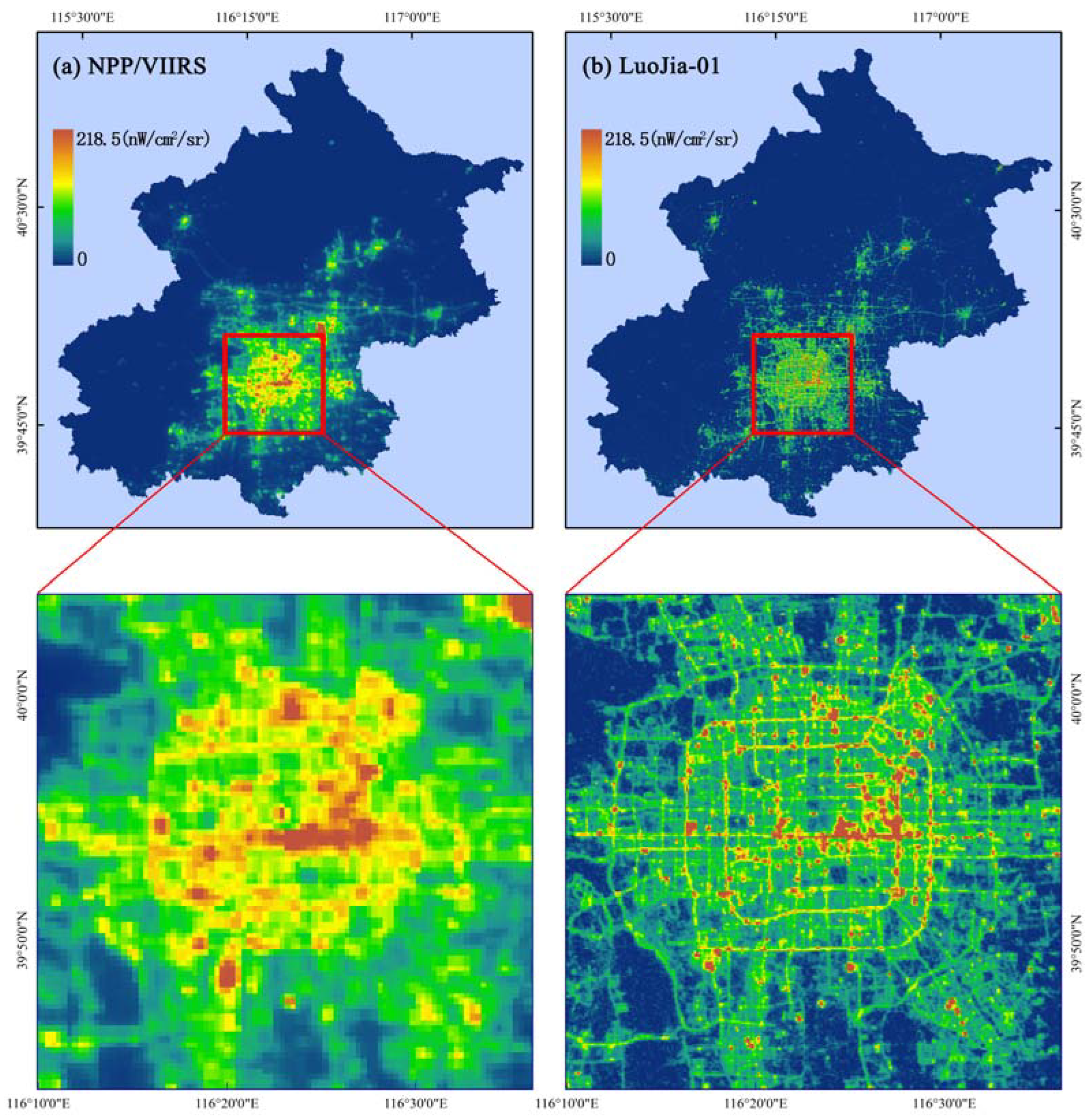
Figure 1. Map of the study areas (zoomed-in Beijing city center, red voxes) and NTL datasets. (a,b) Overall spatial distributions of the NPP-VIIRS NTL data (September 2018) and LuoJia1-01 NTL data (September 2018).
Remotesensing 14 06400 g001
Figure 3. Scatter density plots between the estimated and actual NTL values for each pixel between (a) MGWR, (b) GWR, and the (c) RF regression.
Remotesensing 14 06400 g003
Figure 4. Spatial images showing the comparison of the results of the three downscaling methods in the zoomed-in Beijing city center, (a) LuoJia-01, (b) NPP/VIIRS, (c) MGWR, (d) GWR, (e) RF. (Spatial resolution: 500 m; study period: September 2018).
Remotesensing 14 06400 g004
Figure 5. Spatial texture contrast maps of the downscaled NTL data predicted by the three methods. The red boxes indicate the location of the local area within the entire study area. (a) Beijing Capital International Airport; (b) part of Central Beijing. Study period: September 2018.
Remotesensing 14 06400 g005
Figure 6. Maps depicting the validation areas (HR and FS) and NTL datasets. (a,b) Overall spatial distributions of the NPP-VIIRS NTL data (September 2018) and LuoJia1-01 NTL data (September 2018).
Remotesensing 14 06400 g006
Figure 7. Spatial images comparing of the results of the three downscaling methods in the HR region, (a) LuoJia-01, (b) NPP/VIIRS, (c) MGWR, (d) GWR, (e) RF. (Spatial resolution: 500 m; study period: September 2018).
Remotesensing 14 06400 g007
Figure 8. Spatial images comparing results of the three downscaling methods in the FS region, (a) LuoJia-01, (b) NPP/VIIRS, (c) MGWR, (d) GWR, (e) RF. (Spatial resolution: 500 m; study period: September 2018).
Remotesensing 14 06400 g008
Table 1. Sensors and basic parameters of NTL data.
Remote Sensing PlatformAvailable TimeData ProductsSpatial
Resolution (m)
Temporal Resolution
DMSP-OLS1992–2013Stable lights~10001 year
NPP-VIIRSApril 2012–presentMonthly cloud-free composites5001 month
19 January 2012–presentNightly mosaics7501 day
EROS-B2013–presentRaw data0.7ordering
JL1-3BJanuary 2017–presentRaw data0.92ordering
LuoJia1-01June 2018–2019Raw data~13015 days
Table 2. Attributes of data used in this study.
Data TypeData Acquisition TimeSpatial Resolution (m)Wavelengths (μm)Data Format
Landsat 8 OLI
Landsat 8 TIRS
August–September 201830
100
0.43–1.38
10.60–12.51
GeoTIFF
NPP-VIIRS Monthly cloud-free DNB compositeSeptember 20185000.5–0.9GeoTIFF
LuoJia1-01September 20181300.46–0.98GeoTIFF
LUCC201830/GeoTIFF
Road densitySeptember 2018120/GeoTIFF
POISeptember 2018//ShapeFile
Table 3. Statistics of regression coefficients for MGWR simulation.
Auxiliary VariablesNDVINDBILUCCRoad DensityPOI DensityLSTIntercept
PCC−0.27−0.120.170.280.290.15/
Mean−0.951−0.023−0.0040.0700.3870.0232.148
STD−0.1530.0120.0250.0960.3580.1420.598
Min−2.086−0.052−0.135−0.350−1.219−0.5170.857
Median−1.036−0.025−0.0010.0590.3060.0122.039
Max−0.028−0.0030.0650.9122.4741.7054.240
Table 4. Difference between GWR and MGWR bandwidth settings.
Auxiliary VariablesNDVINDBILUCCRoad DensityPOI DensityLSTIntercept
MGWR bandwidth4370755848435043
GWR bandwidth70707070707070
Table 5. Difference between the regression relationships of NTL and POI data at various resolution scales.
Spatial
Resolution (m)
All Image PixelsCentral City Pixels
CoefficientInterceptCoefficientIntercept
120 m28.1672.6720.66363.23
240 m26.5878.2220.50367.57
360 m26.2580.1320.42371.24
480 m26.2280.1920.32379.28
600 m24.7483.6819.35384.42
Publisher’s Note: MDPI stays neutral with regard to jurisdictional claims in published maps and institutional affiliations.