Article

A Large-Scale Invariant Matching Method Based on DeepSpace-ScaleNet for Small Celestial Body Exploration

1
National Space Science Centre, Chinese Academy of Sciences, Beijing 100190, China
2
University of Chinese Academy of Sciences, Beijing 100049, China
3
School of Fundamental Physics and Mathematical Sciences, Hangzhou Institute for Advanced Study, UCAS, Hangzhou 310024, China
*
Author to whom correspondence should be addressed.
Remote Sens. 2022, 14(24), 6339; https://doi.org/10.3390/rs14246339
Submission received: 23 October 2022 / Revised: 8 December 2022 / Accepted: 8 December 2022 / Published: 14 December 2022
(This article belongs to the Section Satellite Missions for Earth and Planetary Exploration)

Abstract

:
Small Celestial Body (SCB) image matching is essential for deep space exploration missions. In this paper, a large-scale invariant method is proposed to improve the matching accuracy of SCB images under large-scale variations. Specifically, we designed a novel network named DeepSpace-ScaleNet, which employs an attention mechanism for estimating the scale ratio to overcome the significant variation between two images. Firstly, the Global Attention-DenseASPP (GA-DenseASPP) module is proposed to refine feature extraction in deep space backgrounds. Secondly, the Correlation-Aware Distribution Predictor (CADP) module is built to capture the connections between correlation maps and improve the accuracy of the scale distribution estimation. To the best of our knowledge, this is the first work to explore large-scale SCB image matching using Transformer-based neural networks rather than traditional handcrafted feature descriptors. We also analysed the effects of different scale and illumination changes on SCB image matching in the experiment. To train the network and verify its effectiveness, we created a simulation dataset containing light variations and scale variations named Virtual SCB Dataset. Experimental results show that the DeepSpace-ScaleNet achieves a current state-of-the-art SCB image scale estimation performance. It also shows the best accuracy and robustness in image matching and relative pose estimation.

1. Introduction

With the development of deep space exploration technology, future Small Celestial Body (SCB) probes require highly autonomous detection capability for intelligent exploration in deep space [1,2,3]. The extraction and matching of image features are the basis and prerequisite for autonomous visual navigation, and their accuracy directly affects the accuracy and performance of navigation.
Before landing, the probes need to observe the SCB from orbit, take photographs of the SCB’s surface and extract image features manually or automatically. Position estimation and navigation are achieved by matching these reference image features during the landing phase [4,5]. Images taken during the comet characterisation and close observation phases were applied to the landing phase, as shown in Figure A1 (in Appendix A) of the Rosetta mission [6]. However, deep space differs from ground-based scenes because the altitude changes dramatically from orbiting to landing. There are two difficulties with the image matching of the SCB: (1) The images have enormous scale feature variations. For example, in the Hayabusa2 mission, the SCB surface image taken at 20 km altitude is very different from 500 m altitude [5]. When the SCB is photographed from a great distance, the SCB occupies only a few tens of pixels in the whole image. (2) In the process of SCB exploration, the illumination of the reference and navigation images varies considerably. Variations in image features such as scale and illumination affect the robustness of the matching, further affecting the accuracy of the navigation.
Existing matching methods for SCB images focus on traditional methods such as feature points and interest regions [7], line features [8] and crater matching [9,10,11]. These methods work most of the time, but the accuracy will decrease if the scale and lighting are very different. In many computer vision tasks, some feature detection and matching methods based on deep learning have shown their effectiveness [12,13]. Unfortunately, the above methods are not designed for extreme scale changes, so they perform poorly when the images change massively during deep space exploration [14,15]. For the problem of scale changes, the multi-scale feature extraction method based on image pyramids can extract the feature levels in the neighbourhood to find the correspondence of image pairs [15,16,17]. However, the image pyramid layers are limited. For two images with large-scale variations, it is possible that the extracted multi-scale local features are not correlated, resulting in the correct correspondence not being obtained [15]. Some methods of estimating the scale ratio between two images have been proposed to solve this problem and improve the matching accuracy [14,15,18,19]. The main principle is to adjust the unrelated scale levels to be related by first estimating the scale ratio and then matching the images. However, the largest scale ranges that these methods can address are also unsuitable for challenging SCB scenarios.
To overcome these limitations, this paper proposes the DeepSpace-ScaleNet and integrates it into our proposed large-scale invariant matching method. DeepSpace-ScaleNet is a scale estimation network adapted to the SCB scene to improve the effect of image matching more effectively. The DeepSpace-ScaleNet architecture includes two modules, GA-DenseASPP module and CADP module. The former incorporates channel and spatial information through a global attention mechanism. Meanwhile, the dense connectivity of ASPP is used to extract features for large-scale scenes. The latter uses the Transformer to capture the connections between two correlation maps and improve the accuracy of the scale distribution estimation. With these two modules, we have improved the overall performance of the algorithm. Our proposed approach effectively addresses the critical shortcomings of state-of-the-art methods. As shown in Figure 1, it can significantly improve the performance of local features under large-scale changes in images.
The main contributions of this paper are as follows:
(1)
As far as we know, we are the first to propose a solution to the problem of matching images of SCB with large-scale variations.
(2)
We have creatively used scale estimation networks in SCB image matching and designed DeepSpace-ScaleNet by using the architecture of Transformer. This is unprecedented in previous SCB matching methods.
(3)
We designed the novel GA-DenseASPP module and CADP module in DeepSpace-ScaleNet, which can improve the performance of the algorithm.
(4)
We created the first simulated SCB dataset named Virtual SCB Dataset in the field, which can be applied to image matching, relative localization and more.
The rest of this article is organized as follows. In Section 2, we describe the related work image local feature detection and multi-scale modules, especially in deep space. Section 3 describes the SCB image matching method, including DeepSpace-ScaleNet. Section 4 introduces the Virtual SCB Dataset we created and applied to this work. Section 5 and Section 6 evaluate the experimental simulation and give the conclusions of this paper, respectively.

2. Related Work

Image local features widely used in the deep space scene can provide important reference information for SCB navigation, yet they also face significant challenges. One of the major challenges is matching images with large-scale variations because the surface appearance at lower altitudes differs significantly from those at high altitudes. Table A1 in Appendix B briefly summarises some representative technical approaches and our method.

2.1. Local Feature Extraction and Matching

Feature-based pipelines generally follow feature detection, description and matching [20,21]. Some traditional manual feature detection algorithms such as Harris [22] and FAST [23] are based on corner point detection, which aligns with an intuitive understanding of features. However, these methods cannot be applied when large-scale changes exist. The blob speckle-based SIFT [24] and its modified version SURF [25] introduce the DOG-based scale space theory and solve the problems of target rotation, scaling and lighting changes to some extent. After the feature spot is detected, the area around the feature needs to be described with a feature vector. The SIFT descriptor describes the feature with a 128-dimensional vector, while ORB [26] uses a binary, which is much faster. The most essential feature point matching method is Brute-force (BF) matching, and later the Flann-based matcher was utilized for efficiency [27]. Deep learning-based feature detection methods have also been proposed in recent years. Key. Net extracts manual feature points over multiple-scale layers via CNN to solve the problem of the lack of true annotation of features [28]. LF-Net proposes a new deep feature extraction framework and trains the method by known relative poses and correspondences [29]. SuperPoint is a feature point detection and descriptor extraction method based on self-supervised training [12]. It adopts a self-learning method to avoid extensive manual annotations and has stronger robustness to seasons, lighting, etc. SuperGlue uses graph neural networks to match features [13]. Thanks to its added attention to contextual aggregation mechanisms, it can learn the geometric transformations and conventional a priori knowledge of the 3D world. LOFTR proposes a coarse-to-fine local dense feature matching method that achieves better results in weakly textured regions [30].
Currently, there are fewer methods specifically for SCB image feature detection. The existing methods are generally based on the above standard local feature extraction and matching approaches for navigation and surface reconstruction. Due to the lack of training data, most researchers still use traditional manual features. For example, Takeishi, N. et al. evaluated the performance of several common feature detection and description methods and found that the performance of SIFT is acceptable [7]. Nonetheless, SIFT also fails to match when large-scale changes occur in the image [5]. In addition to interest points, more advanced features such as line features [8,31], shadow features [32] and craters [9,10,11] on the surface of SCB are also used for SCB navigation. The primary methods for SCB image matching are feature point-based and pattern matching [33]. The feature point-based approach provides a straightforward and efficient matching process through the distance between the two descriptors [34,35]. Pattern matching uses the image land markers extracted from the observed images to match the features with the land markers in the reference terrain library [33,36]. The craters are extracted from the images taken during the landing of the probe, and pattern matching is performed with a reference database based on features such as the crater’s edge, diameter, relative distance and angle to obtain information on the absolute position and attitude of the probe [37,38,39,40]. However, many landmark features seen in high orbits cannot be observed again in low orbits because the altitude of the space probe has changed. For example, as the probe descends, the number of craters in view decreases. Therefore, it is necessary to propose a matching method suitable for large-scale changes in SCB images.

2.2. Image Scale Estimation

To address the image matching problem caused by large-scale changes, Zhou et al. proposed a scale-invariant image matching approach SLM-BOF, inspired by the scale space theory, to tackle the extensive scale changes [18]. In 2021, Fu et al. introduced a learning-based network to estimate the scale ratio, which has much higher accuracy than SLM-BOF [15]. By contrast, ScaleNet outputs a scale distribution in logarithmic space rather than a regressed single scale ratio, which helps the network converge to a reliable model [14]. In addition, the image box embedding that approximates the visible surface overlap measures is used to estimate the scale ratio between two images [19]. Unfortunately, the above methods can only estimate scale ratios within restricted limits due to the gaping differences between deep space and ground scenes. However, they cannot satisfy the requirements of SCB missions. To overcome these limitations, we proposed DeepSpace-ScaleNet better to achieve the large-scale invariant matching of SCB images.

2.3. Multi-Scale Modules

How to capture multi-scale context is an important issue in computer vision tasks. In deep space, as shown in Figure 1, the SCB may occupy only a few or even one pixel in the image during the fly-around phase. However, it may occupy half or more image pixels during the landing phase. Therefore, this process requires special modules to capture the multi-scale context.
Image pyramids are the typical method to capture multi-scale contexts by fusing multiple resized input images [16,17,41,42,43,44]. However, the major limitation of such networks is that they consume vast amounts of GPU memory, which is almost impractical for lightweight SCB probes.
Networks with encoder-decoder architecture fuse features of different resolutions produced by different layers [45,46,47,48]. In the encoder, the resolution of the input image is gradually reduced, and the deep feature maps have larger receptive fields. In the decoder, the resolution of the image is gradually recovered, and the shallow feature maps have more object details. PSPNet proposed the pyramid pooling module (PPM) to capture features at several grid scales [49]. The ASPP and its follow-ups expand the receptive field by parallel atrous convolution layers of different dilation rates [50,51,52,53]. Deformable convolution is proposed in [54,55] to focus on pertinent image regions. In [56], they proposed Receptive Field Block (RFB), which combines a multi-branch convolution layer and dilated pooling or convolution layer, imitating the structure of RF in human visual systems. A pyramidally attended feature extraction module (PAFE) was constructed to make multi-scale features more attention-enhanced in [57]. How to design multi-scale modules for deep space imagery is the question to be considered.

3. Methods

As shown in Figure 1, extracting critical points between two images with different scales is challenging, resulting in poor performance of image matching methods. The deep space scene is a typical example, where the number of pixels occupied by the SCB is different between the orbiting phase and the landing phase of the probe. To solve the problem, we proposed a large-scale invariant method for SCB image matching and designed the DeepSpace-ScaleNet for estimating the scale of the SCB images photographed in the two phases mentioned above.

3.1. Large-Scale Invariant Method for SCB Image Matching

The percentage of SCB pixels in the image field varies a lot when the probes are at different orbital altitudes of the SCB. Traditional image pyramid-based multi-scale feature extraction methods consider only a few adjacent scale layers [15]. It leads to the following problems: on the one hand, the feature descriptors generated from the two feature pyramids are too different to correspond; on the other hand, multi-scale feature extraction methods may cause the SCB to be almost drowned out by the background noise in the upper-level features map, which is also a significant challenge in computer vision.
Consequently, our approach suggests predicting the scale ratio before image matching to overcome the above limitations. As in Figure 2, the scale ratio between Images A and B is predicted by DeepSpace-ScaleNet. Both images were resized according to this ratio before subsequent images were matched. For example, the scale ratio for Images A and B is S. When S is greater than 1, it means that the size of the SCB in Image A is S times larger than in Image B. Therefore, we upsample Image B by a ratio of S and match it with Image A. When S is less than 1, the image of Image A is sampled on the image by a ratio of S.

3.2. Scale Distributions

ScaleNet formulates the scale estimation as a probability distribution prediction and experimentally demonstrates the effectiveness of probability distribution predictions relative to regression models [14].
Inspired by it, our DeepSpace-ScaleNet outputs a probability distribution of length L . Given two images, the final scale ratio is calculated by the following. Estimate the scale distribution s A B i weighted by the predicted scale probabilities p i from ImageA to ImageB. The same operation is performed for ImageB to ImageA. Equation (1) computes the scale ratios S A B and S B A , and they are inverse. We combine them as S ^ A B and calculate the final scale factor between the images S A B .
S A B = i = 0 L 1 p i log σ ( s A B i ) ,   S B A = i = 0 L 1 p i log σ ( s B A i )
S ^ A B = S A B S B A 2
S A B = σ S ^ A B

3.3. DeepSpace-ScaleNet

To tackle the problems mentioned in the abstract, we propose DeepSpace Scalenet, which fills the gap of scale estimation for deep space scenes. Compared with several state-of-the-art methods via comprehensive experiments, Deepspace-Scalenet can estimate more accurate scales.

3.3.1. Deepspace-Scalenet Architecture

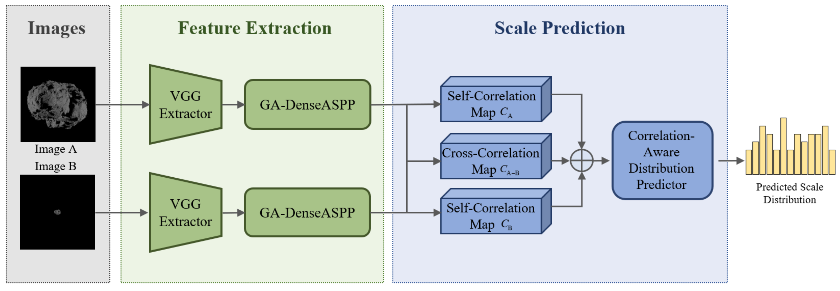
As shown in Figure 3, DeepSpace-ScaleNet accepts ImageA and ImageB as input. The features are first extracted by a pre-trained model and then passed through the GA-DenseASPP module. Specifically, the global attention mechanism fuses the channel and spatial information, and the multi-scale information is obtained by atrous convolution. After that, the refined features are processed by the method [58] to obtain self-correlation maps, C A , C B and cross-correlation maps C A B . Finally, the three correlation maps are concatenated in the channel dimension and fed into the CADP to output scale distribution.
As shown in Figure 3, our proposed method uses a similar architecture as ScaleNet [14]. However, it replaces the modules of ScaleNet with more efficient ones, making the network more applicable to multi-scale scenes such as deep space backgrounds. We introduce two Crucial modules: Global Attention-DenseASPP (GA-DenseASPP) and Correlation-aware Distribution Predictor (CADP).

3.3.2. Global Attention-DenseASPP (GA-DenseASPP)

The attention mechanism [59,60,61,62,63] has been widely used in computer vision tasks such as feature extraction and semantic segmentation. The global attention mechanism [59] captures both channel and spatial information and magnifies salient cross-dimension receptive regions. To extract multi-scale information accurately, we proposed GA-DenseASPP.
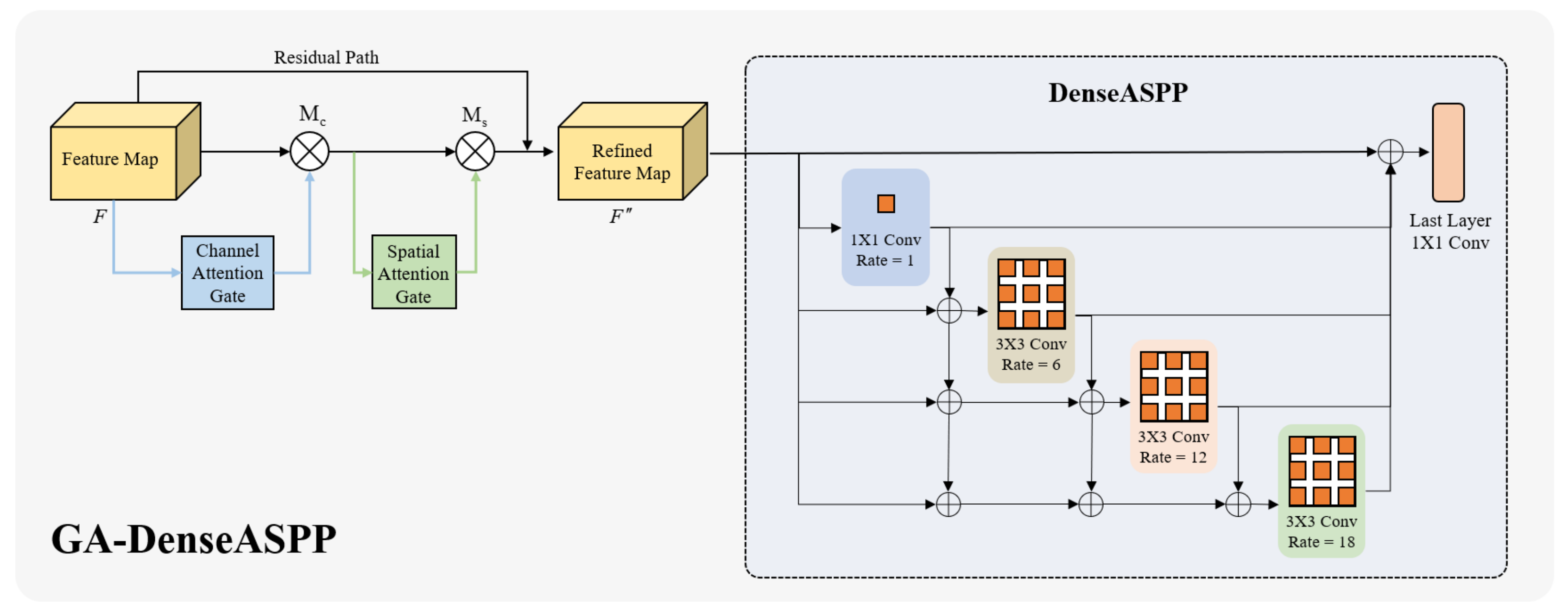
As shown in Figure 4, we take the feature map F R 512 × H × W as input, where 512 , H , W indicates the channels, height and width of F , respectively. Then, the GAM [59] processes the feature map and refines it through the channel attention gate and spatial attention gate, respectively, which can better explore the channel and spatial relationship of the feature map. The above-mentioned process is formulated in Equations (4) and (5).
F = M c F F
F = M s F F
where F and F are channel-refined and spatial-refined feature maps, respectively; M c and M s are attention maps of the channel and spatial module, respectively; denotes element-wise multiplication.
Finally, the final refined feature map is fed into Dense Atrous Spatial Pyramid Pooling (DenseASPP). Dense Atrous Spatial Pyramid Pooling consists of a cascade of atrous convolution layers that can encode multi-scale information from feature maps through dense connections.
Compared with the ASPP used in ScaleNet, GA-DenseASPP is more efficient for multi-scale scenes such as deep space, and can accurately extract information from features of different scales.
The feature map extracted by the pre-trained model is fused with spatial and channel information by GAM. Then, it is fed into a cascade of atrous convolution layers of DenseASPP.
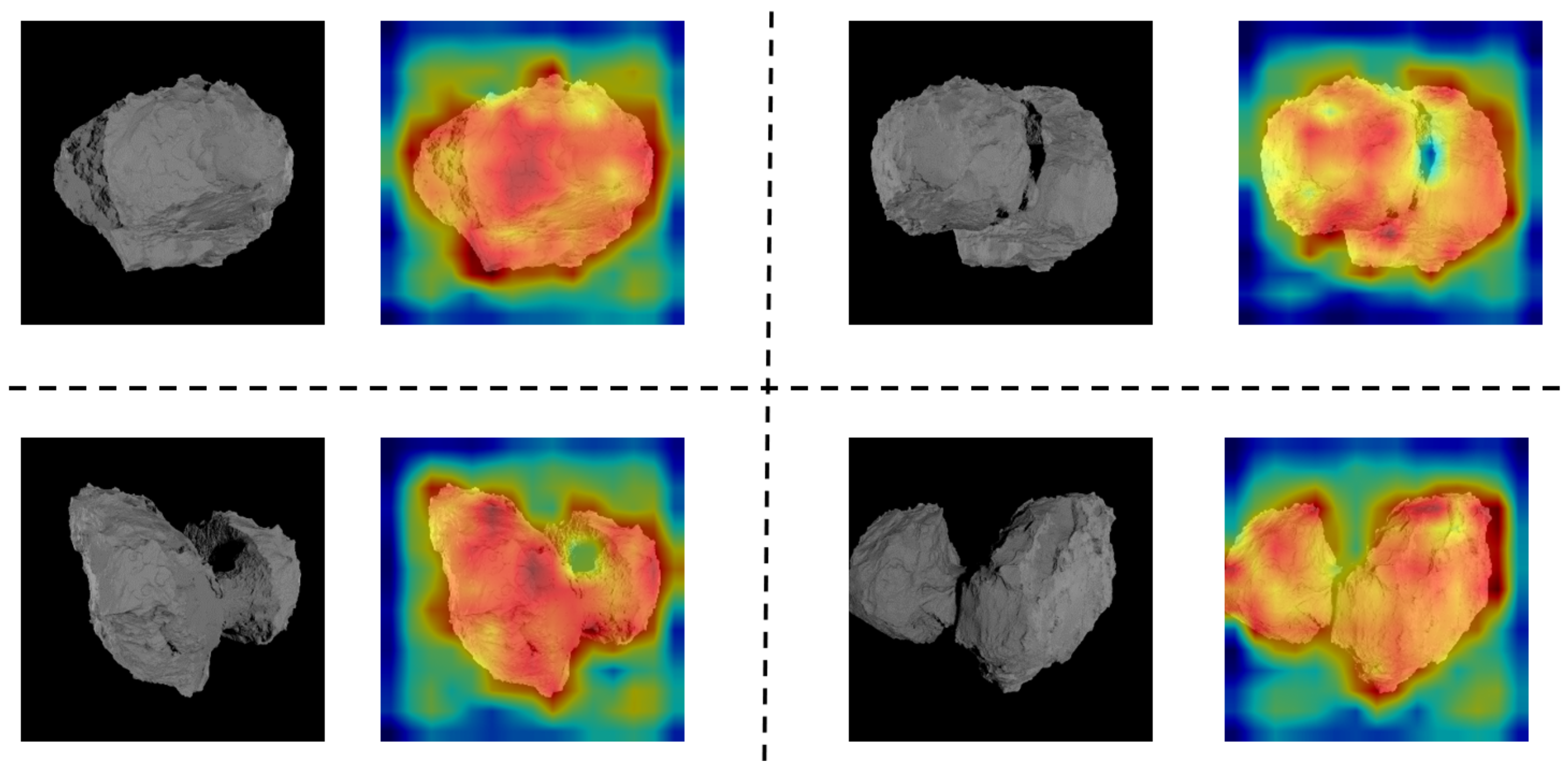
The attention mechanism is added to DeepSpace-ScaleNet as an effective module. We use Grad-CAM [64] to visualize the feature maps in Figure 5. It takes the gradient of the predicted scale ratios flowing into the attention module to produce feature visualizations, highlighting regions that contribute highly to scale estimation. As shown in Figure 5, the network pays more attention to the visible textures on the SCB surface and selectively ignores the deep space background and the invisible areas of the SCB surface. The attention module enables the network to extract image features that are useful for prediction and helps it output a more accurate scale distribution.

3.3.3. Correlation-aware Distribution Predictor (CADP)

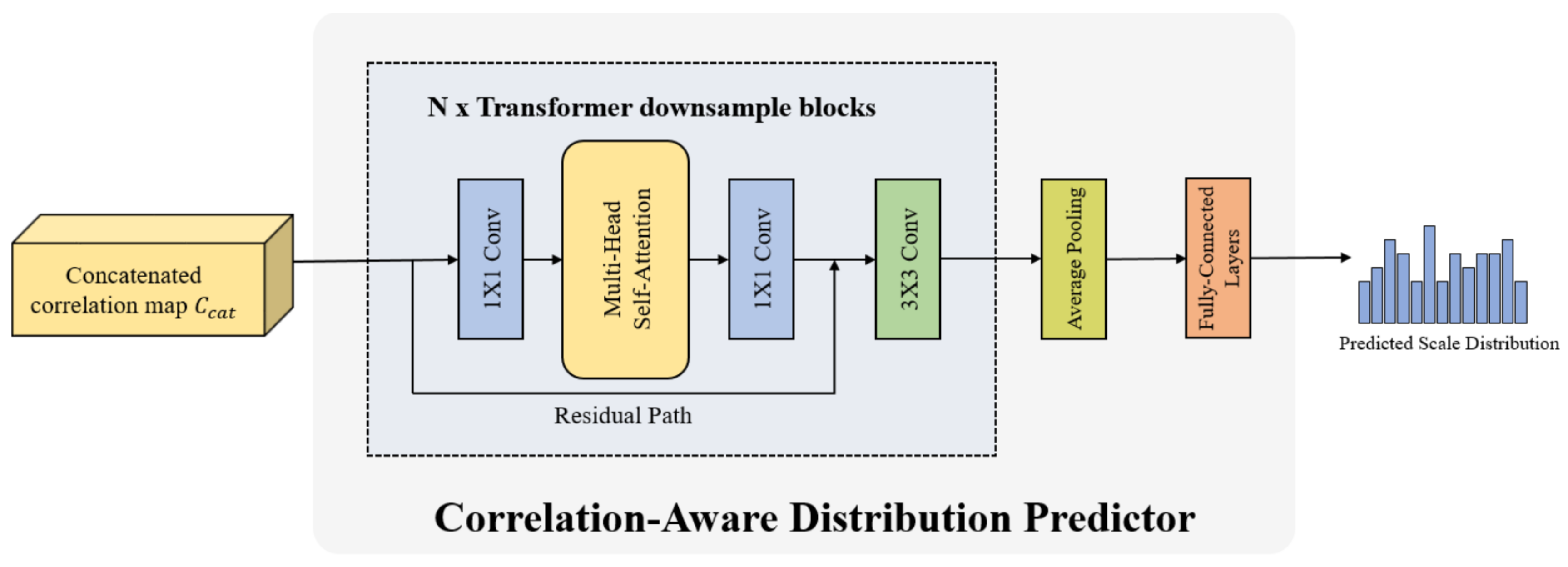
The fully connected layers cannot capture the inner relationship between correlation maps, so this may lead to inaccurate scale estimation. To solve this problem, we proposed CADP module. It consists of a few stacked Transformer downsample blocks, an average pooling layer and a set of fully connected layers. The efficiency of the Transformer has been demonstrated in many computer vision tasks, as its multi-head self-attention layer can integrate information from the entire image, even at the lowest layers [51].
As shown in Figure 6, CADP takes the concatenated correlation map as input, indicating the channels, height and width C c a t , respectively. Then, C c a t is fed to Transformer downsample blocks to integrate the inner relationship in correlation maps and reduce its shape gradually. After that, the downsampled correlation map is forward fed into an average pooling layer, and its height and width are reduced to 1. Finally, it is flattened and processed by a set of fully connected layers to predict scale distribution.
The Transformer downsample block is based on the BoTNet [65]. The number of Transformer downsample blocks is N. The block consists of two 1 × 1 convolution layers, a multi-head self-attention layer and ends with a 3 × 3 convolution layer. The multi-head self-attention layer can capture long-range dependencies across the entire correlation maps, but it requires a lot of computational resources to train. For a trade-off between the accuracy of scale estimation and computational efficiency of multi-head self-attention, we use 1 × 1 convolution layer to reduce the channel of the concatenated correlation map. For the same reason as above, we set the stride of the 3 × 3 convolution layer to 2. Each convolution layer is followed by a batch normalization layer [66] and an activation layer.
Compared with only fully connected layers in ScaleNet, CADP is more correlation-aware. Our experiments demonstrate that it is an effective and efficient module to capture the relationship between correlation maps.

3.3.4. Loss Function

We use the Kullback–Leibler divergence loss function to measure the distance between predicted scale distribution P A B and ground-truth distribution P g t A B .
L oss ( A , B ) = K L ( P A B , P g t A B )

3.3.5. Learning Rate and Optimizer

The learning rate plays an essential role in the model’s training as a necessary parameter of the neural network. The model needs a large learning rate in the first few epochs to perform a sharper and faster gradient descent. As the epoch grows, the model needs a small learning rate to stabilize the convergence process. The decay ratio can control the learning rate to decrease gradually with the growth of the epoch.
Therefore, setting an appropriate learning rate and decay ratio determines the accuracy of the model prediction. We set the initial learning rate to 10 4 , and the learning rate decays when it reaches 5, 15, 25 and 35 with a decay ratio of 0.1.
As for the optimizer, we chose Stochastic gradient descent (SGD). Because the SGD is more suitable than Adam for extended experiments, another advantage of SGD is that it reduces the computational burden remarkably and speeds up the iterative process of each epoch.

4. Virtual SCB Dataset

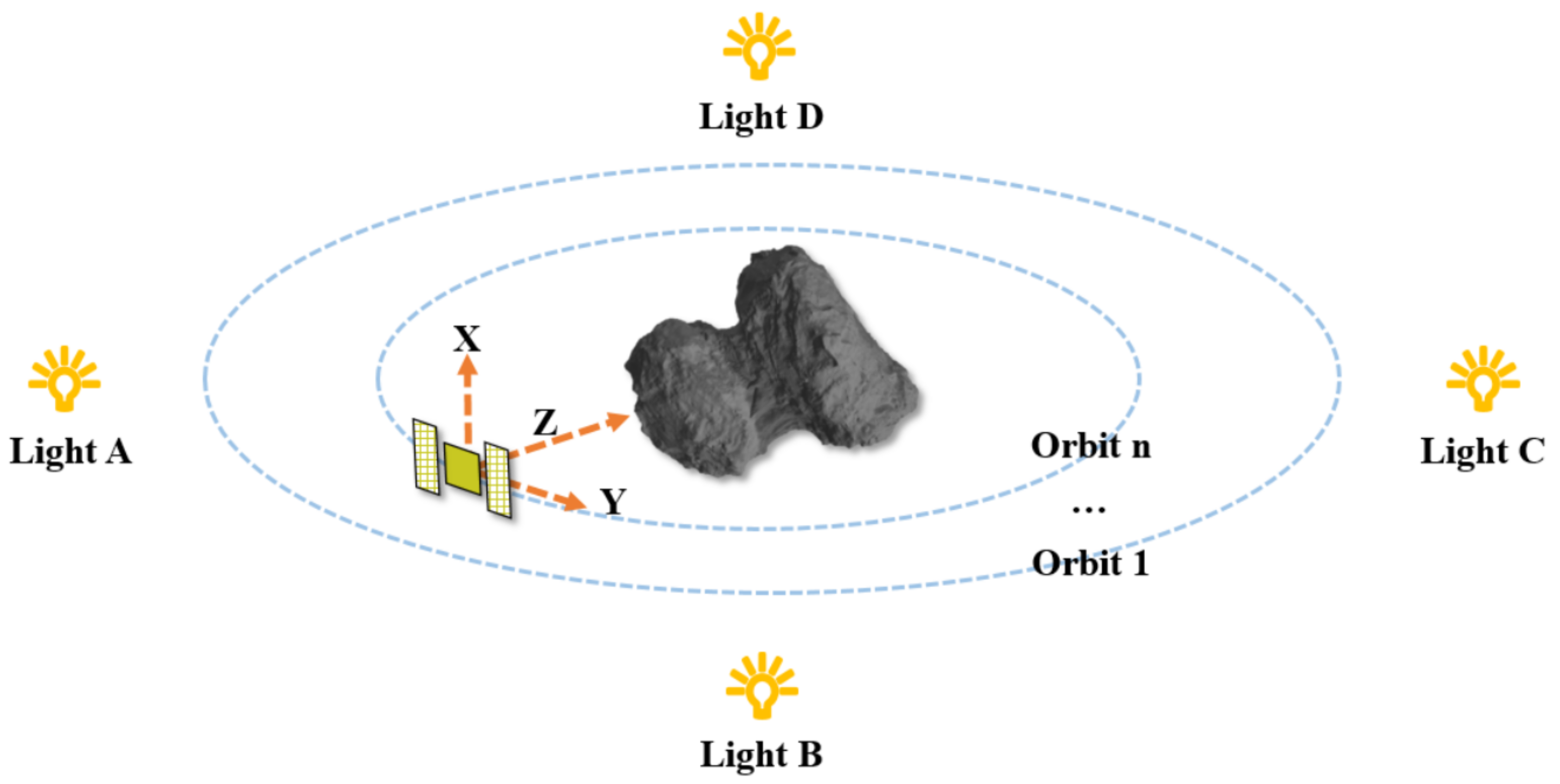
Considering that there are only images from the SCB exploration mission, there is a lack of public datasets available for feature detection and scale estimation. We use Blender to generate the SCB image dataset. Blender is an open-source 3D simulation engine that supports the use of python scripts. The three-dimensional SCB models used in this paper are 67P/Churyumov–Gerasimenko [67] and Ryugu [68]. The specific process is shown in Figure 7. The SCB’s centre of mass is used as the origin of the world coordinate system. Four light sources are placed near the SCB to simulate the camera’s images in different sunshine conditions. Images are taken when the camera is placed at different orbital heights in order to take images at different scales. The camera’s Z-axis always points to the SCB to ensure that the SCB is in the centre of the image. The camera is moved at each height, and 51 images are taken to ensure sufficient overlap between adjacent images. The resolution of the camera is set to 1024 × 1024 pixels.
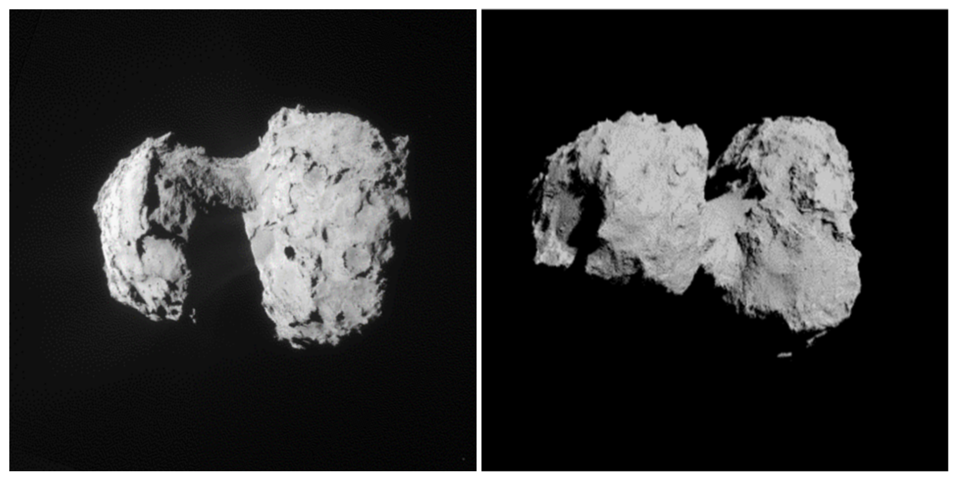
Figure 8 shows the real 67 P image (left) and our simulated image (right). Compared with the real image, the texture and shadow of the simulated image are very realistic and can reflect the surface characteristics of the real image.
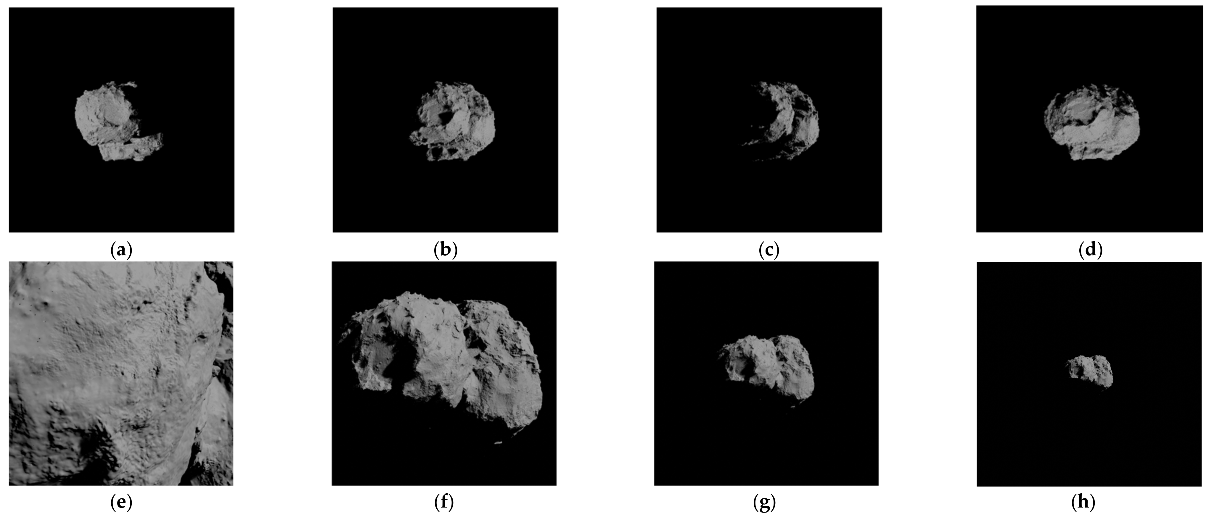
Figure 9a–d shows simulated images of SCB with different illumination from the same viewing angle; (e–h) are SCB shot at different altitudes (4, 10, 20, 40 km). The observation shows that when the illumination and scale change drastically, the surface characteristics of the SCB change significantly.
The altitude range of our generated SCB images is (5150) km. A set of images was generated at 5 km intervals, with 51 SCB images in each set. When we generated image pairs, each image was paired with one to three images from other altitudes with adjacent shooting angles. As shown in Table 1, we generated 9145 pairs of images and divided the dataset into four scale ratio ranges. During the training and testing of DeepSpace-ScaleNet, 6655 pairs were used for training, 864 pairs for validation and 1626 pairs for testing. To estimate the impact of lighting on matching, we divide the dataset into a FixedLight Dataset and a VariableLight Dataset according to whether the paired lighting conditions change.

5. Experiments and Results

5.1. Implementation Details

DeepSpace-ScaleNet accepts images of arbitrary size as input. In this work, these images are resized to 240 × 240 and then fed into the network for training. Considering the true scale distribution of our dataset in the range [0.05, 20], we set L = 13 bins and σ = 2.
The dilation rate of DenseASPP is set to {1, 6, 12, 18}, and the number N of the Transformer Downsample Module is set to 2.
Our data augmentation includes flip, rotation and colour augmentation. All our experiments are run on RTX 3080 GPU. It uses a pre-trained VGG model as the feature extractor. The batch size is set to 48. The network is trained at about 50 epochs. The whole training process takes about 1 h.

5.2. Image Scale Estimation

In this section, we compare DeepSpace-ScaleNet with other state-of-the-art methods to demonstrate the effectiveness of our method. We use a learning-based model ScaleNet [14], and a physics-based method named BoundingBoxes Algorithm.
In contrast to the relative scale estimation problem in ScaleNet [14], a large proportion of the SCB images are of a prominent target on a black deep-space background. To verify whether detecting only the target bounding box is an effective estimator of the scale factor, we use Rembg [68] (a phenomenal artificial intelligence-based background remover). It removes the deep space background, segments foreground objects and then detects the bounding box to estimate the image scale difference by comparing the change in the scale of the external frame between the two images.
The evaluation metrics include the average L1 discrepancy E 1 [15] and the average abs discrepancy E 2 . The E 1 was first proposed in [15] to calculate the difference between truth scale ratios and predicted scale ratios. Since E 1 is not sensitive enough for large-scale image pairs of deep space scenes, we propose the E 2 , which enables the evaluation to focus on image pairs with large-scale differences.
The evaluation metrics mentioned above are formulated in Equations (7) and (8).
The average L1 discrepancy E 1 :
E 1 = 1 N i = 1 N log 2 s i log 2 s ^ i
The average abs discrepancy E 2 :
E 2 = 1 N i = 1 N s i s ^ i
where S and S ^ are ground truth scale ratio and predicted scale ratio, respectively. N is the number of image pairs.
Table 2 is a quantitative comparison of the average abs discrepancy and average L1 discrepancy on Virtual SCB Dataset test images. The smaller the error, the more accurate the proportion estimate. It can be seen that DeepSpace-ScaleNet achieves excellent performance under different scales. An order of magnitude improves the estimation accuracy of our proposed model compared with other state-of-the-art methods. Under small scales (1 < s ≤ 5 or 1 < 1 s ≤ 5), the accuracy of the BoundingBoxes algorithm is slightly better than our method. The outer outline of the SCB is visible when the scale difference is negligible, making it easier to use BoundingBoxes to estimate the scale. However, the whole SCB or part of the SCB can fill the image field of view when the scale becomes large. As shown in Table 3c,d, this causes the BoundingBoxes algorithm to be inaccurate. Moreover, ScaleNet is generally better than the BoundingBoxes algorithm, especially at the large-scale level, where it shows a good deal of strength. However, it is still not accurate enough compared to our method. In particular, the accuracy improvement of the proposed method is more significant under large scales (15 < s ≤ 20 or 15 < 1 s ≤ 20). The results verify that DeepSpace-ScaleNet is more suitable for large-scale backgrounds such as deep space scenes.
The qualitative results of scale estimation are shown in Table 3. Image pairs were taken from test sets under different scales. As we can see, DeepSpace-ScaleNet is more robust to changes in illumination and changes in viewpoint than other methods, resulting in a more accurate scale distribution.

5.3. Ablation Study

In this section, several ablation experiments were conducted to demonstrate the effectiveness of the above modules. The same parameters were used in all experiments. The evaluation metrics included the average L1 discrepancy [15] E 1 and the average abs discrepancy E 2 .
We used ASPP to replace GA-DenseASPP. The dilation rates of both were set to 1 , 6 , 12 , 18 .
We used the fully connected layers to replace CADP.
The effectiveness of our proposed module for scale estimation can be seen in Table 4. Our proposed GA-DenseASPP is more effective for deep space scenes, which can extract multi-scale information accurately. Then, CADP can integrate the inner relationship of the correlation maps, which is more correlation-aware than the fully connected layers.

5.4. Image Matching

In this section, we conducted image matching experiments using the Virtual SCB Dataset and compared the matching results with and without DeepSpace-ScaleNet. The combination method of SIFT [24] (extraction method) + FLANN [27] (matching method) and the combination method of SuperPoint [12] (extraction method) + SuperGlue [13] (matching method) were used to extract image features and match images. Notably, the former combination method is the most representative traditional-based method, and the latter is a state-of-the-art learning-based approach.
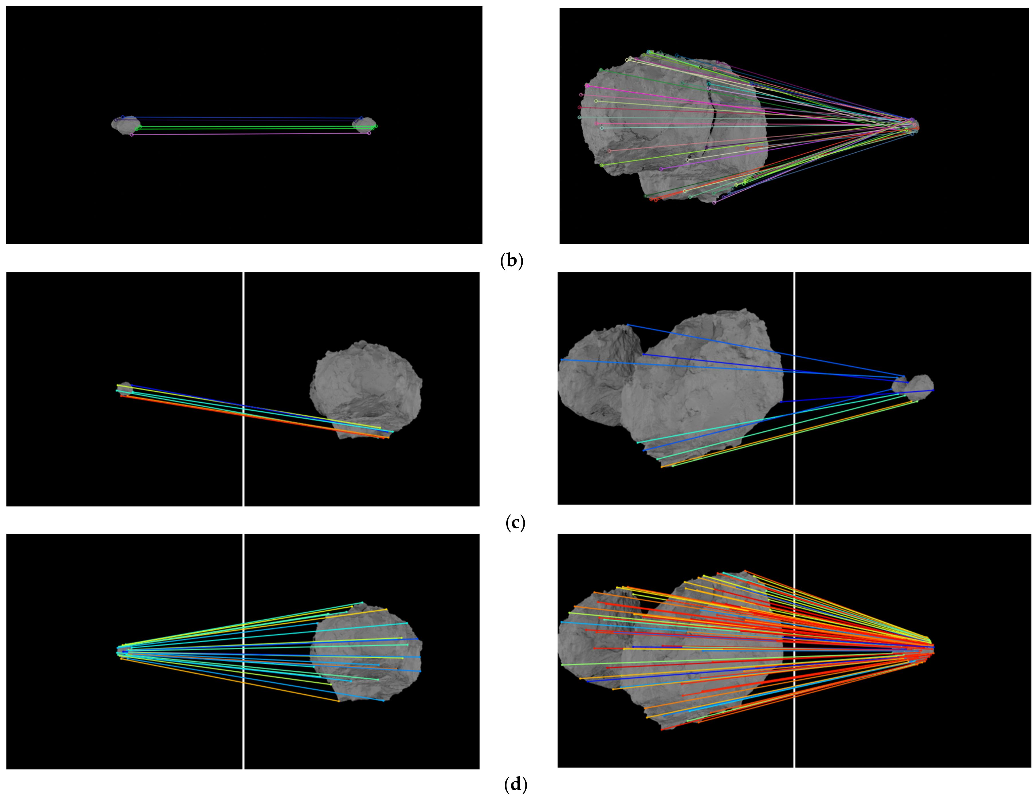
In Figure 10, we present our image matching visualization results. When DeepSpace-ScaleNet is not used, SIFT + FLANN and SuperPoint + SuperGlue suffer from an insufficient number of matching points and incorrect matching point correspondence. In contrast, the performance of matching points improves significantly with DeepSpace-ScaleNet. Not only are there more matching pairs, but also the accuracy has increased. The experimental results show that the proposed method can efficiently mitigate the problem under large-scale variation and outperform state-of-the-art approaches in image matching.
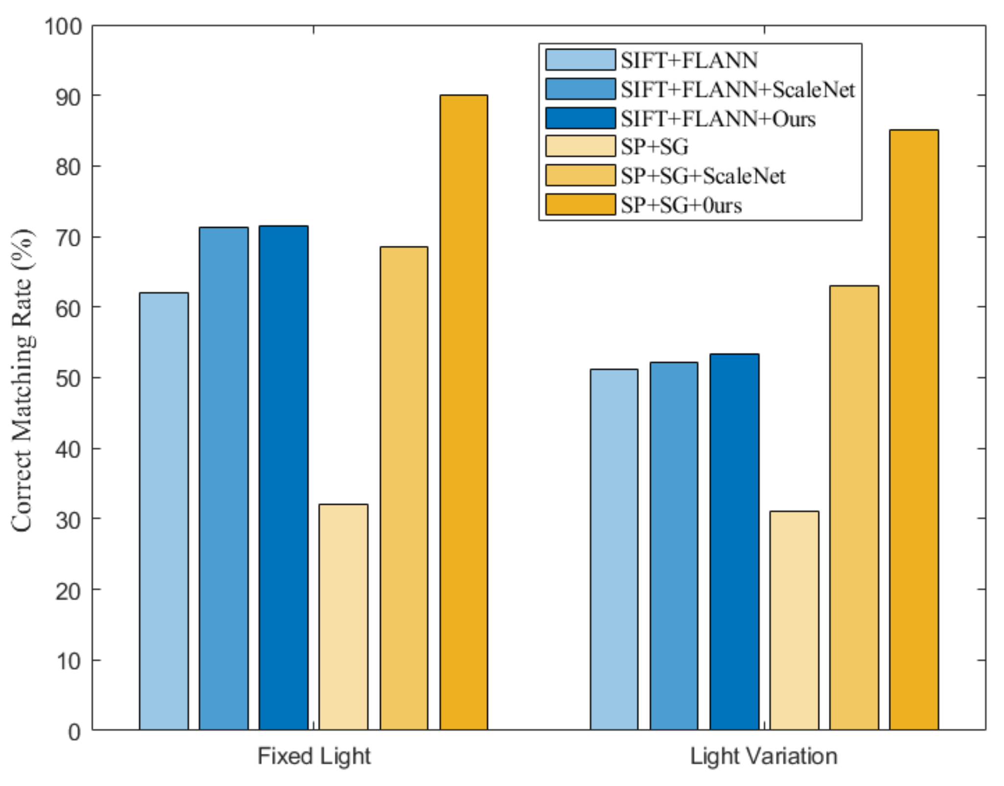
To further analyse the contribution of DeepSpace-ScaleNet, several experiments were conducted in the FixedLight Dataset and VariableLight Dataset. We use the Correct Matching Rate to calculate the matching accuracy of each algorithm when the number of feature point matching pairs corresponding to two images is greater than a certain threshold, which is considered a correct matching pair. After matching all the pairs of images, the Correct Matching Rate is used to calculate the matching accuracy of each algorithm [14]. N A l l   M a t c h i n g   P a i r s is all matching pairs in the dataset and N C o r r e c t   M a t c h i n g   P a i r s is the number of all correct matching pairs.
C o r r e c t   M a t c h i n g   R a t e = N ( C o r r e c t   M a t c h i n g   P a i r s ) N ( A l l   M a t c h i n g   P a i r s ) × 100 %
Figure 11 demonstrates that the performance of both the matching methods improved after combining DeepSpace-ScaleNet. SuperPoint + SuperGlue + DeepSpace-ScaleNet even achieved matching rates of 90.04 and 85.06%, indicating that only a small number of images failed to be matched correctly. ScaleNet also proved to be effective, indicating that the combined scale estimation method is indeed meaningful for image matching. Also, a comparison of results using two different datasets shows that SuperPoint + SuperGlue is somewhat robust to illumination but less invariant to scale. This is also in line with our experience. The experimental results show that state-of-the-art matching results can be achieved when combined with DeepSpace-ScaleNet.

5.5. Relative Pose Estimation

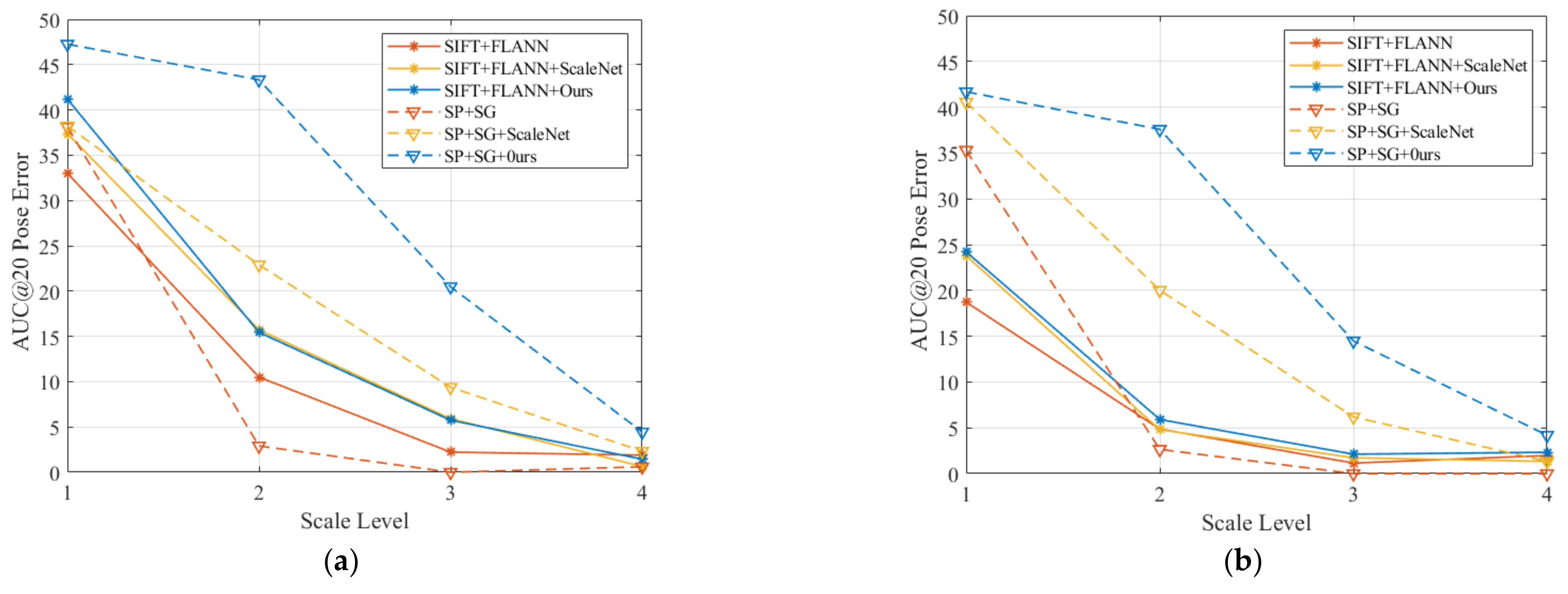
In SCB exploration missions, matching image pairs are obtained primarily for relative pose estimation. In this section, we evaluate the impact of the DeepSpace-ScaleNet on the relative pose estimation of SCB images. As in 5.4, SIFT + FLANN and SuperPoint + SuperGlue were selected as image extraction and matching methods. Specifically, we compared the AUC of the pose error at the thresholds (5, 10, 20°) calculated by SIFT and FLANN and SuperPoint and SuperGlue with and without DeepSpace-ScaleNet in the FixedLight Dataset and VariableLight Dataset.
The AUC of the pose error is the maximum of the angular errors in rotation and translation, which is often used in existing positional error estimates [13,30]. Table 5 and Table 6 report the errors of pose estimation in the FixedLight Dataset and the VariableLight Dataset. As we can see, outstanding improvements are achieved when combined with DeepSpace-ScaleNet. At AUC@20, an improvement of 182.21% can be obtained compared to a single-scale approach such as SuperPoint + SuperGlue. Compared to ScaleNet, the method proposed in this paper works better and achieves the best results in all experimental results. Meanwhile, SIFT + FLANN also has a 35.96% improvement. In addition, SIFT outperforms SuperPoint + SuperGlue in both @5@10@20 when the light environment is stable and the opposite in the light-varying dataset.
Figure 12 shows the error of the relative pose estimation for each matching method without combining the scale estimation method and with combining ScaleNet and the proposed method DeepSpace-ScaleNet in this paper, respectively. The dataset was divided into four scale levels for analysis according to the dataset partitioning in Section 4. Figure 12a indicates the error at the FixedLight Dataset. SuperPoint + SuperGlue outperforms SIFT + FLANN when the scale range is below level 1 (1 < s ≤ 5 or 1 < 1 s ≤ 5). This is because the former has better generalization performance. However, once the scale variation exceeds level 1 (1 < s ≤ 5 or 1 < 1 s ≤ 5), the performance of SuperPoint + SuperGlue drops steeply, as SIFT + FLANN is more robust to large-scale variation. When combined with DeepSpace-ScaleNet, the performance of both is improved. In particular, SuperPoint + SuperGlue shows a significant improvement. This result suggests that DeepSpace-ScaleNet can improve the accuracy of relative pose estimation, especially in large-scale variation. Thus, adding scale estimation can lead to good results for single-scale estimation networks without the need to recreate the data for training. Furthermore, one phenomenon that can be observed is that DeepSpace-ScaleNet achieves better results than ScaleNet. Figure 12b shows the situation on the VariableLight Dataset. Comparing the same coloured line segments in Figure 12 shows that the matching accuracy decreases when the illumination level changes. Specifically, SIFT is less robust to illumination, while SuperPoint + SuperGlue is more robust to illumination changes. Combined with the method proposed in this paper, the performance of both is improved.

6. Conclusions

This paper proposed a large-scale invariant method-based DeepSpace-ScaleNet for SCB image matching at large-scale and light variations. Our proposed network improves image matching accuracy at scale and illumination variations by estimating the scale ratio of the two images. On the one hand, the proposed approach has better feature extraction capability for large-scale deep space scenes while estimating more accurate scale distributions. On the other hand, this mechanism of first estimating the image scale and then resizing and matching the image is more suitable for SCB exploration. The results demonstrate its superiority in that it can correctly boost the performance of all the matching methods when the scale and lighting of the image are substantially changed. The method proposed in this paper could potentially be applied to future deep space exploration missions in China, including the autonomous navigation of SCB probes and 3D reconstruction. We will explore a more lightweight and efficient network of widely used onboard processors in the future.

Author Contributions

Conceptualization, M.F.; Methodology, M.F. and W.L.; Software, M.F. and W.L.; Validation, M.F. and W.L.; Formal analysis, M.F. and W.L.; Investigation, M.F. and W.L.; Resources, W.N. and X.P.; Data curation, M.F. and W.L.; Writing—original draft, M.F. and W.L.; Writing—review and editing, M.F. and W.N.; Visualization, M.F.; Supervision, W.N., X.P. and Z.Y.; Project administration, W.N., X.P. and Z.Y.; Funding acquisition, W.N. and X.P. All authors have read and agreed to the published version of the manuscript.

Funding

This work was partly supported by the Youth Innovation Promotion Association under Grant E1213A02, and the Key Research Program of Frontier Sciences, CAS, Grant NO. 22E0223301.

Institutional Review Board Statement

Not applicable.

Informed Consent Statement

Informed consent was obtained from all subjects involved in the study.

Data Availability Statement

Not applicable.

Conflicts of Interest

The authors declare no conflict of interest.

Appendix A

In May 2014, Rosetta entered the comet phase of its mission. It approached comet 67/P Churyumov–Gerasimenko, characterised it, deployed the lander and orbited around the comet collecting scientific observations. As shown in Figure A1, the operations were split into the following phases: Comet approach, Comet characterisation, Comet global mapping, Close observation, Lander delivery and Extended monitoring [6].
DeepSpace-ScaleNet in this paper can be applied in the landing phase. During the characterisation phase, the spacecraft observes the comet at a distance of between 90 and 120 km and takes a large number of images to identify the comet’s surface landmarks. Higher-resolution images are taken between 10 and 20 km during the approach phase. During the landing phase, our method can be used to match images and estimate the location of the spacecraft.
Figure A1. Rosetta mission operational phase.
Remotesensing 14 06339 g0a1

Appendix B

Table A1. A summary of some representative technical methods and our methods.
Research Field in Deepspace ExplorationRelated WorkThe AdvantagesThe DisadvantagesOur Contributions
(Proposing a New Method)
Image Local Feature Extraction And Matching SIFT [24] + FLANN [27] A robust performance to scale changesNot available when scene lighting changes dramaticallyMore robust to changes in light
SuperPoint [12] + SuperGlue [13]A robust performance to changes in lightInability to adapt to large-scale changesMore robust to large-scale changes
Pattern matching based on meteorite craters, etc. [9,10,11]Suitable for SCB ScenariosDeactivated when there are no craters in the field of viewNo requirement for craters, rocks, etc., in the field of view, and a wide range of application
Estimation Of Image Scale RatioScaleNet [14]Valid for most scale changesLow accuracy in deep space scenesHigher accuracy of scale estimation in deep space scenes
Multi-scale ModulesImage feature pyramids [16,17,41,42,43,44]Ability to overcome scale changesLimits to computational efficiencyMore lightweight
ASPP [50,51,52,53] Ability to extract multi-scale features in the networkLimited by deeper featuresBetter extraction of large-scale scene features

References

  1. Ge, D.; Cui, P.; Zhu, S. Recent development of autonomous GNC technologies for small celestial body descent and landing. Prog. Aerosp. Sci. 2019, 110, 100551. [Google Scholar] [CrossRef]
  2. Song, J.; Rondao, D.; Aouf, N. Deep learning-based spacecraft relative navigation methods: A survey. Acta Astronaut. 2022, 191, 22–40. [Google Scholar] [CrossRef]
  3. Ye, M.; Li, F.; Yan, J.; Hérique, A.; Kofman, W.; Rogez, Y.; Andert, T.P.; Guo, X.; Barriot, J.P. Rosetta Consert Data as a Testbed for in Situ Navigation of Space Probes and Radiosciences in Orbit/Escort Phases for Small Bodies of the Solar System. Remote Sens. 2021, 13, 3747. [Google Scholar] [CrossRef]
  4. Zhong, W.; Jiang, J.; Ma, Y. L2AMF-Net: An L2-Normed Attention and Multi-Scale Fusion Network for Lunar Image Patch Matching. Remote Sens. 2022, 14, 5156. [Google Scholar] [CrossRef]
  5. Anzai, Y.; Yairi, T.; Takeishi, N.; Tsuda, Y.; Ogawa, N. Visual localization for asteroid touchdown operation based on local image features. Astrodynamics 2020, 4, 149–161. [Google Scholar] [CrossRef]
  6. de Santayana, R.P.; Lauer, M. Optical measurements for rosetta navigation near the comet. In Proceedings of the 25th International Symposium on Space Flight Dynamics (ISSFD), Munich, Germany, 19–23 October 2015. [Google Scholar]
  7. Takeishi, N.; Tanimoto, A.; Yairi, T.; Tsuda, Y.; Terui, F.; Ogawa, N.; Mimasu, Y. Evaluation of Interest-Region Detectors and Descriptors for Automatic Landmark Tracking on Asteroids. Trans. Jpn. Soc. Aeronaut. Space Sci. 2015, 58, 45–53. [Google Scholar] [CrossRef] [Green Version]
  8. Shao, W.; Cao, L.; Guo, W.; Xie, J.; Gu, T. Visual navigation algorithm based on line geomorphic feature matching for Mars landing. Acta Astronaut. 2020, 173, 383–391. [Google Scholar] [CrossRef]
  9. DeLatte, D.M.; Crites, S.T.; Guttenberg, N.; Yairi, T. Automated crater detection algorithms from a machine learning perspective in the convolutional neural network era. Adv. Space Res. 2019, 64, 1615–1628. [Google Scholar] [CrossRef]
  10. Cheng, Y.; Johnson, A.E.; Matthies, L.H.; Olson, C.F. Optical landmark detection for spacecraft navigation. Adv. Astronaut. Sci. 2003, 114, 1785–1803. [Google Scholar]
  11. Kim, J.R.; Muller, J.-P.; van Gasselt, S.; Morley, J.G.; Neukum, G. Automated crater detection, a new tool for Mars cartography and chronology. Photogramm. Eng. Remote Sens. 2005, 71, 1205–1217. [Google Scholar] [CrossRef] [Green Version]
  12. DeTone, D.; Malisiewicz, T.; Rabinovich, A. Superpoint: Self-supervised interest point detection and description. In Proceedings of the IEEE Conference on Computer Vision and Pattern Recognition Workshops, Salt Lake City, UT, USA, 18–22 June 2018; pp. 224–236. [Google Scholar]
  13. Sarlin, P.E.; Detone, D.; Malisiewicz, T.; Rabinovich, A. Superglue: Learning feature matching with graph neural networks. In Proceedings of the IEEE/CVF Conference on Computer Vision and Pattern Recognition, Seattle, WA, USA, 14–29 June 2020; pp. 4938–4947. [Google Scholar]
  14. Barroso-Laguna, A.; Tian, Y.; Mikolajczyk, K. ScaleNet: A Shallow Architecture for Scale Estimation. In Proceedings of the IEEE/CVF Conference on Computer Vision and Pattern Recognition, Nashville, TN, USA, 20–25 June 2022; pp. 12808–12818. [Google Scholar]
  15. Fu, Y.; Zhang, P.; Liu, B.; Rong, Z.; Wu, Y. Learning to Reduce Scale Differences for Large-Scale Invariant Image Matching. IEEE Trans. Circuits Syst. Video Technol. 2022, 61, 583–592. [Google Scholar] [CrossRef]
  16. Lin, T.-Y.; Dollár, P.; Girshick, R.; He, K.; Hariharan, B.; Belongie, S. Feature Pyramid Networks for Object Detection. In Proceedings of the IEEE Conference on Computer Vision and Pattern Recognition, Honolulu, HI, USA, 21–26 July 2017; pp. 2117–2125. [Google Scholar]
  17. Ghiasi, G.; Fowlkes, C.C. Laplacian Pyramid Reconstruction and Refinement for Semantic Segmentation. In Proceedings of the European Conference on Computer Vision, Amsterdam, The Netherlands, 11–14 October 2016; Springer: Cham, Switzerland, 2016; pp. 519–534. [Google Scholar]
  18. Zhou, L.; Zhu, S.; Shen, T.; Wang, J.; Fang, T.; Quan, L. Progressive large-scale-invariant image matching in scale space. In Proceedings of the IEEE International Conference on Computer Vision, Venice, Italy, 22–29 October 2017; pp. 2362–2371. [Google Scholar]
  19. Rau, A.; Garcia-Hernando, G.; Stoyanov, D.; Brostow, G.J.; Turmukhambetov, D. Predicting visual overlap of images through interpretable non-metric box embeddings. In Proceedings of the European Conference on Computer Vision, Glasgow, UK, 23–28 August 2020; Springer: Cham, Switzerland, 2020; pp. 629–646. [Google Scholar]
  20. Jiang, X.; Ma, J.; Xiao, G.; Shao, Z.; Guo, X. A review of multimodal image matching: Methods and applications. Inf. Fusion 2021, 73, 22–71. [Google Scholar] [CrossRef]
  21. Ma, J.; Jiang, X.; Fan, A.; Jiang, J.; Yan, J. Image matching from handcrafted to deep features: A survey. Int. J. Comput. Vis. 2021, 129, 23–79. [Google Scholar] [CrossRef]
  22. Harris, C.; Stephens, M. A combined corner and edge detector. Alvey Vis. Conf. 1988, 15, 10–5244. [Google Scholar]
  23. Rosten, E.; Drummond, T. Machine learning for high-speed corner detection. In Proceedings of the European Conference on Computer Vision, Graz, Austria, 7–13 May 2006; Springer: Berlin, Heidelberg, 2006; pp. 430–443. [Google Scholar]
  24. Lowe, D.G. Distinctive image features from scale-invariant keypoints. Int. J. Comput. Vis. 2004, 60, 91–110. [Google Scholar] [CrossRef]
  25. Bay, H.; Ess, A.; Tuytelaars, T.; Gool, L. Speeded-up robust features (SURF). Comput. Vis. Image Underst. 2008, 110, 346–359. [Google Scholar] [CrossRef]
  26. Rublee, E.; Rabaud, V.; Konolige, K.; Bradski, G. ORB: An efficient alternative to SIFT or SURF. In Proceedings of the 2011 International Conference on Computer Vision, Barcelona, Spain, 6–13 November 2011; pp. 2564–2571. [Google Scholar] [CrossRef]
  27. Yang, L.; Huang, Q.; Li, X.; Yuan, Y. Dynamic-scale grid structure with weighted-scoring strategy for fast feature matching. Appl. Intell. 2022, 52, 10576–10590. [Google Scholar] [CrossRef]
  28. Laguna, A.B.; Riba, E.; Ponsa, D.; Mikolajczyk, K. Key.Net: Keypoint Detection by Handcrafted and Learned CNN Filters. Proc. IEEE Int. Conf. Comput. Vis. 2019, 2019, 5835–5843. [Google Scholar] [CrossRef] [Green Version]
  29. Ono, Y.; Fua, P.; Trulls, E.; Yi, K.M. LF-Net: Learning Local Features from Images. Adv. Neural Inf. Process. Syst. 2018, 2018, 6234–6244. [Google Scholar]
  30. Sun, J.; Shen, Z.; Wang, Y.; Bao, H.; Zhou, X. LoFTR: Detector-free local feature matching with transformers. In Proceedings of the IEEE/CVF Conference on Computer Vision and Pattern Recognition, Nashville, TN, USA, 21–24 June 2021; pp. 8922–8931. [Google Scholar]
  31. Shao, W.; Gu, T.; Ma, Y.; Xie, J.; Cao, L. A Novel Approach to Visual Navigation Based on Feature Line Correspondences for Precision Landing. J. Navig. 2018, 71, 1413–1430. [Google Scholar] [CrossRef]
  32. Matthies, L.; Huertas, A.; Cheng, Y.; Johnson, A. Stereo Vision and Shadow Analysis for Landing Hazard Detection. In Proceedings of the 2008 IEEE International Conference on Robotics and Automation, Pasadena, CA, USA, 19–23 May 2008; pp. 2735–2742. [Google Scholar] [CrossRef]
  33. Wang, Y.; Yan, X.; Ye, Z.; Xie, H.; Liu, S.; Xu, X.; Tong, X. Robust Template Feature Matching Method Using Motion-Constrained DCF Designed for Visual Navigation in Asteroid Landing. Astrodynamics 2023, 7, 83–99. [Google Scholar] [CrossRef]
  34. Johnson, A.E.; Cheng, Y.; Matthies, L.H. Machine vision for autonomous small body navigation. In Proceedings of the 2000 IEEE Aerospace Conference. Proceedings (Cat. No. 00TH8484), Big Sky, MT, USA, 25 March 2000; Volume 7, pp. 661–671. [Google Scholar]
  35. Cocaud, C.; Kubota, T. SLAM-based navigation scheme for pinpoint landing on small celestial body. Adv. Robot. 2012, 26, 1747–1770. [Google Scholar] [CrossRef]
  36. Cheng, Y.; Miller, J.K. Autonomous landmark based spacecraft navigation system. In Proceedings of the 2003 AAS/AIAA Astrodynamics Specialist Conference, Big Sky, MT, USA, 13–17 August 2003. [Google Scholar]
  37. Yu, M.; Cui, H.; Tian, Y. A new approach based on crater detection and matching for visual navigation in planetary landing. Adv. Space Res. 2014, 53, 1810–1821. [Google Scholar] [CrossRef]
  38. Cui, P.; Gao, X.; Zhu, S.; Shao, W. Visual Navigation Using Edge Curve Matching for Pinpoint Planetary Landing. Acta Astronaut. 2018, 146, 171–180. [Google Scholar] [CrossRef]
  39. Tian, Y.; Yu, M. A novel crater recognition based visual navigation approach for asteroid precise pin-point landing. Aerosp. Sci. Technol. 2017, 70, 1–9. [Google Scholar] [CrossRef]
  40. Xiao, T.; Liu, Y.; Zhou, B.; Jiang, Y.; Sun, J. Unified Perceptual Parsing for Scene Understanding. In Proceedings of the Proceedings of the European conference on computer vision (ECCV), Munich, Germany, 8–14 September 2018; pp. 418–434. [Google Scholar]
  41. Eigen, D.; Fergus, R. Predicting depth, surface normals and semantic labels with a common multi-scale convolutional architecture. In Proceedings of the IEEE International Conference on Computer Vision, Santiago, Chile, 7–13 December 2015; pp. 2650–2658. [Google Scholar]
  42. Farabet, C.; Couprie, C.; Najman, L.; LeCun, Y. Learning Hierarchical Features for Scene Labeling. IEEE Trans. Pattern Anal. Mach. Intell. 2012, 35, 1915–1929. [Google Scholar] [CrossRef] [Green Version]
  43. Lin, G.; Shen, C.; Van Den Hengel, A.; Reid, I. Efficient piecewise training of deep structured models for semantic segmentation. In Proceedings of the IEEE Conference on Computer Vision and Pattern Recognition, Las Vegas, NV, USA, 27–30 June 2016; pp. 3194–3203. [Google Scholar]
  44. Ronneberger, O.; Fischer, P.; Brox, T. U-net: Convolutional networks for biomedical image segmentation. In Proceedings of the International Conference on Medical Image Computing and Computer-Assisted Intervention, Munich, Germany, 5–9 October 2015; Springer: Cham, Switzerland, 2015; pp. 234–241. [Google Scholar]
  45. Pohlen, T.; Hermans, A.; Mathias, M.; Leibe, B. Full-resolution residual networks for semantic segmentation in street scenes. In Proceedings of the IEEE Conference on Computer Vision and Pattern Recognition, Honolulu, HI, USA, 21–26 July 2017; pp. 4151–4160. [Google Scholar]
  46. Amirul Islam, M.; Rochan, M.; Bruce, N.D.B.; Wang, Y. Gated feedback refinement network for dense image labeling. In Proceedings of the IEEE Conference on Computer Vision and Pattern Recognition, Honolulu, HI, USA, 21–26 July 2017; pp. 3751–3759. [Google Scholar]
  47. Oktay, O.; Schlemper, J.; Le Folgoc, L.; Lee, M.; Heinrich, M.; Misawa, K.; Mori, K.; McDonagh, S.; Hammerla, N.Y.; Kainz, B. Attention U-Net: Learning Where to Look for the Pancreas. arXiv 2018, arXiv:arXiv1804.03999. [Google Scholar]
  48. Zhao, H.; Shi, J.; Qi, X.; Wang, X.; Jia, J. Pyramid scene parsing network. In Proceedings of the IEEE Conference on Computer Vision and Pattern Recognition, Honolulu, HI, USA, 21–26 July 2017; pp. 2881–2890. [Google Scholar]
  49. Chen, L.-C.; Papandreou, G.; Kokkinos, I.; Murphy, K.; Yuille, A.L. Deeplab: Semantic Image Segmentation with Deep Convolutional Nets, Atrous Convolution, and Fully Connected Crfs. IEEE Trans. Pattern Anal. Mach. Intell. 2017, 40, 834–848. [Google Scholar] [CrossRef] [Green Version]
  50. Chen, L.-C.; Papandreou, G.; Schroff, F.; Adam, H. Rethinking atrous convolution for semantic image segmentation. arXiv 2017, arXiv:1706.05587. [Google Scholar]
  51. Chen, L.-C.; Zhu, Y.; Papandreou, G.; Schroff, F.; Adam, H. Encoder-decoder with atrous separable convolution for semantic image segmentation. In Proceedings of the European Conference on Computer Vision (ECCV), Munich, Germany, 8–14 September 2018; pp. 801–818. [Google Scholar]
  52. Zhao, X.; Pang, Y.; Zhang, L.; Lu, H.; Zhang, L. Suppress and balance: A simple gated network for salient object detection. In Proceedings of the European Conference on Computer Vision, Glasgow, UK, 23–28 August 2020; Springer: Cham, Switzerland, 2020; pp. 35–51. [Google Scholar]
  53. Dai, J.; Qi, H.; Xiong, Y.; Li, Y.; Zhang, G.; Hu, H.; Wei, Y. Deformable Convolutional Networks. In Proceedings of the IEEE International Conference on Computer Vision, Venice, Italy, 22–29 October 2017; pp. 764–773. [Google Scholar]
  54. Zhu, X.; Hu, H.; Lin, S.; Dai, J. Deformable Convnets V2: More Deformable, Better Results. In Proceedings of the IEEE Computer Society Conference on Computer Vision and Pattern Recognition, Long Beach, CA, USA, 16–20 June 2019; pp. 9300–9308. [Google Scholar]
  55. Liu, S.; Huang, D. Receptive field block net for accurate and fast object detection. In Proceedings of the European conference on computer vision (ECCV), Munich, Germany, 8–14 September 2018; pp. 385–400. [Google Scholar]
  56. Zhao, X.; Zhang, L.; Pang, Y.; Lu, H.; Zhang, L. A single stream network for robust and real-time RGB-D salient object detection. In Proceedings of the European Conference on Computer Vision, Glasgow, UK, 23–28 August 2020; Springer: Cham, Switzerland, 2020; pp. 646–662. [Google Scholar]
  57. Rocco, I.; Arandjelovic, R.; Sivic, J. Convolutional neural network architecture for geometric matching. In Proceedings of the IEEE Conference on Computer Vision and Pattern Recognition, Honolulu, HI, USA, 21–26 July 2017; pp. 6148–6157. [Google Scholar]
  58. Liu, Y.; Shao, Z.; Hoffmann, N. Global Attention Mechanism: Retain Information to Enhance Channel-Spatial Interactions. arXiv 2021, arXiv:2112.05561. [Google Scholar]
  59. Woo, S.; Park, J.; Lee, J.-Y.; Kweon, I.S. Cbam: Convolutional Block Attention Module. In Proceedings of the Proceedings of the European conference on computer vision (ECCV), Munich, Germany, 8–14 September 2018; pp. 3–19. [Google Scholar]
  60. Park, J.; Woo, S.; Lee, J.-Y.; Kweon, I.S. Bam: Bottleneck Attention Module. arXiv 2018, arXiv:1807.06514. [Google Scholar]
  61. Misra, D.; Nalamada, T.; Arasanipalai, A.U.; Hou, Q. Rotate to Attend: Convolutional Triplet Attention Module. In Proceedings of the Proceedings of the IEEE/CVF Winter Conference on Applications of Computer Vision, Virtual, 5–9 January 2021; IEEE: Piscataway, NJ, USA, 2021; pp. 3139–3148. [Google Scholar]
  62. Fukui, H.; Hirakawa, T.; Yamashita, T.; Fujiyoshi, H. Attention branch network: Learning of attention mechanism for visual explanation. In Proceedings of the IEEE/CVF Conference on Computer Vision and Pattern Recognition, Long Beach, CA, USA, 16–20 June 2019; pp. 10705–10714. [Google Scholar]
  63. Selvaraju, R.R.; Cogswell, M.; Das, A.; Vedantam, R.; Parikh, D.; Batra, D. Grad-cam: Visual explanations from deep networks via gradient-based localization. In Proceedings of the IEEE International Conference on Computer Vision, Venice, Italy, 22–29 October 2017; pp. 618–626. [Google Scholar]
  64. Srinivas, A.; Lin, T.-Y.; Parmar, N.; Shlens, J.; Abbeel, P.; Vaswani, A. Bottleneck Transformers for Visual Recognition. In Proceedings of the IEEE/CVF Conference on Computer Vision and Pattern Recognition, Nashville, TN, USA, 20–25 June 2021; IEEE: Piscataway, NJ, USA, 2021; pp. 16519–16529. [Google Scholar]
  65. Ioffe, S.; Szegedy, C. Batch normalization: Accelerating deep network training by reducing internal covariate shift. International conference on machine learning. PMLR 2015, 37, 448–456. [Google Scholar]
  66. Glassmeier, K.H.; Boehnhardt, H.; Koschny, D.; Kührt, E.; Richter, I. The Rosetta Mission: Flying towards the Origin of the Solar System. Space Sci. Rev. 2007, 128, 1–21. [Google Scholar] [CrossRef]
  67. Saiki, T.; Takei, Y.; Fujii, A.; Kikuchi, S.; Terui, F.; Mimasu, Y.; Ogawa, N.; Ono, G.; Yoshikawa, K.; Tanaka, S. Overview of the Hayabusa2 Asteroid Proximity Operations. In Hayabusa2 Asteroid Sample Return Mission; Elsevier: Amsterdam, The Netherlands, 2022; pp. 113–136. [Google Scholar]
  68. Qin, X.; Zhang, Z.; Huang, C.; Dehghan, M.; Zaiane, O.R.; Jagersand, M. U2-Net: Going deeper with nested U-structure for salient object detection. Pattern Recognit. 2020, 106, 107404. [Google Scholar] [CrossRef]
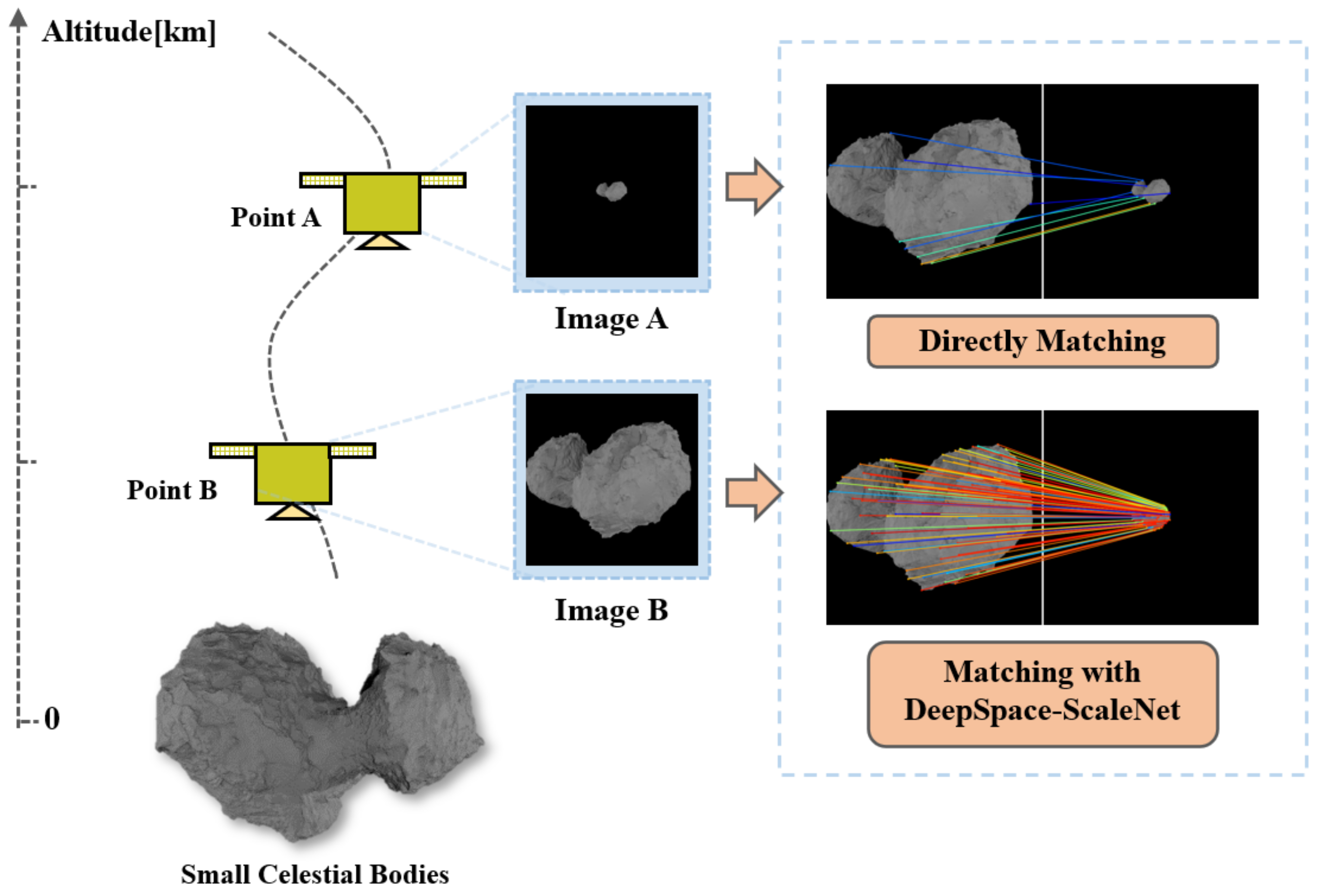
Figure 1. Schematic Diagram Of Image Matching With DeepSpace-ScaleNet During SCB Landing.
Remotesensing 14 06339 g001
Figure 2. The Flowchart of Large-scale Invariant Method for SCB Image Matching.
Remotesensing 14 06339 g002
Figure 3. DeepSpace-ScaleNet Architecture.
Remotesensing 14 06339 g003
Figure 4. GA-DenseASPP Module.
Remotesensing 14 06339 g004
Figure 5. Raw data (left) and Grad-CAM visualizations (right) of the attention module on four different pairs of images taken from the Virtual SCB Dataset. Red regions correspond to high contributions for scale estimation, while blue corresponds to low contributions.
Remotesensing 14 06339 g005
Figure 6. Correlation-aware Distribution Predictor (CADP) Module.
Remotesensing 14 06339 g006
Figure 7. Schematic Diagram of Simulation Image Generation.
Remotesensing 14 06339 g007
Figure 8. Real Image (left). Simulated Image (right).
Remotesensing 14 06339 g008
Figure 9. Images Generated Under Different Lighting and Scale Scenes. (a) light A, (b) light B, (c) light C, (d) light D, (e) 4 km, (f) 10 km, (g) 20 km, (h) 40 km.
Remotesensing 14 06339 g009
Figure 10. Image matching visualization results in the virtual SCB dataset. (a) SIFT + FLANN, (b) SIFT + FLANN + DeepSpace-ScaleNet, (c) SuperPoint + SuperGlue, (d) SuperPoint + SuperGlue + DeepSpace-ScaleNet.
Remotesensing 14 06339 g010aRemotesensing 14 06339 g010b
Figure 11. The correct matching rates in the FixedLight dataset and VariableLight dataset.
Remotesensing 14 06339 g011
Figure 12. The Error of Relative Pose Estimation In The FixedLight Dataset And VariableLight Dataset. (a) FixedLight Dataset, (b) VariableLight Dataset.
Remotesensing 14 06339 g012
Table 1. Virtual SCB Dataset.
Scale Ratio RangeAll 1   <   s 5   or   1   <   1 s   5 5   <   s     10   or   5   <   1 s   10 10   <   s 15   or   10   <   1 s   15 15   <   s 20   or   15   <   1 s     20
Number of Pairs9145227633492265755
Proportion100%30.4%36.6%24.8%8.3%
Table 2. Quantitative comparison of the average abs discrepancy and average L1 discrepancy.
ModelAll 1   <   s   5   or   1   <   1 s     5 5   <   s     10   or   5   <   1 s     10 10   <   s     15   or   10   <   1 s     15 15   <   s     20   or   15   <   1 s     20
BoundingBoxes
Algorithm
1.184/0.2800.036/0.0440.075/0.1501.966/0.4237.556/1.233
ScaleNet0.793/0.1730.104/0.1160.118/0.1301.519/0.1833.933/0.517
DeepSpace-ScaleNet0.203/0.0520.047/0.0530.075/0.0460.410/0.0490.693/0.085
Table 3. Qualitative results of scale estimation of the above-mentioned state-of-the-art methods.
Image PairsGround-TruthBoundingBoxes
Algorithm
ScaleNetDeepSpace-ScaleNet
(a)Remotesensing 14 06339 i001Remotesensing 14 06339 i0021.151.141.321.16
(b)Remotesensing 14 06339 i003Remotesensing 14 06339 i00488.297.238.06
(c)Remotesensing 14 06339 i005Remotesensing 14 06339 i00613.513.4311.4913.53
(d)Remotesensing 14 06339 i007Remotesensing 14 06339 i0081813.0712.7518.02
Table 4. Ablation experiment on different components of DeepSpace-ScaleNet.
Average Absolute DiscrepancyAverage L1 Discrepancy
DeepSpace-ScaleNet
w/o GA-DenseASPP
0.2360.057
DeepSpace-ScaleNet w/o CADP0.2370.061
DeepSpace-ScaleNet0.2030.052
Table 5. Pose estimation in the FixedLight dataset.
AUC@5AUC@10AUC@20
SIFT + FLANN4.467.8814.05
SIFT + FLANN + ScaleNet5.32 (19.34%↑)9.69 (23.02%↑)18.06 (28.56%↑)
SIFT + FLANN + Ours5.55 (24.41%↑)10.50 (33.27%↑)19.10 (35.96%↑)
SP + SG3.656.7312.31
SP + SG + ScaleNet4.97 (36.25%↑)10.56 (56.90%↑)21.84 (77.44%↑)
SP + SG + Ours8.55 (134.25%↑)16.96 (152.01%↑)34.74 (182.21%↑)
Table 6. Pose estimation in the VariableLight dataset.
AUC@5AUC@10AUC@20
SIFT + FLANN2.294.197.59
SIFT + FLANN + ScaleNet3.03 (32.29%↑) 5.18 (23.68%↑)9.18 (20.93%↑)
SIFT + FLANN + Ours3.07 (34.18%↑)5.63 (34.51%↑)9.87 (29.99%↑)
SP + SG3.586.4311.36
SP + SG + ScaleNet5.23 (46.20%↑) 10.42 (62.05%↑)20.63 (81.56%↑)
SP + SG + Ours6.97 (94.79%↑)13.96 (117.10%↑)29.42 (158.93%↑)
Publisher’s Note: MDPI stays neutral with regard to jurisdictional claims in published maps and institutional affiliations.