Multispectral Characteristics of Glacier Surface Facies (Chandra-Bhaga Basin, Himalaya, and Ny-Ålesund, Svalbard) through Investigations of Pixel and Object-Based Mapping Using Variable Processing Routines

Abstract

Fundamental image processing methods, such as atmospheric corrections and pansharpening, influence the signal of the pixel. This morphs the spectral signature of target features causing a change in both the final spectra and the way different mapping methods may assign thematic classes. In the current study, we aim to identify the variations induced by popular image processing methods in the spectral reflectance and final thematic maps of facies. To this end, we have tested three different atmospheric corrections: (a) Quick Atmospheric Correction (QUAC), (b) Dark Object Subtraction (DOS), and (c) Fast Line-of-Sight Atmospheric Analysis of Hypercubes (FLAASH), and two pansharpening methods: (a) Hyperspherical Color Sharpening (HCS) and (b) Gram–Schmidt (GS). WorldView-2 and WorldView-3 satellite images over Chandra-Bhaga Basin, Himalaya, and Ny-Ålesund, Svalbard are tested via spectral subsets in traditional (BGRN1), unconventional (CYRN2), visible to near-infrared (VNIR), and the complete available spectrum (VNIR_SWIR). Thematic mapping was comparatively performed using 12 pixel-based (PBIA) algorithms and 3 object-based (GEOBIA) rule sets. Thus, we test the impact of varying image processing routines, effectiveness of specific spectral bands, utility of PBIA, and versatility of GEOBIA for mapping facies. Our findings suggest that the image processing routines exert an extreme impact on the end spectral reflectance. DOS delivers the most reliable performance (overall accuracy = 0.64) averaged across all processing schemes. GEOBIA delivers much higher accuracy when the QUAC correction is employed and if the image is enhanced by GS pansharpening (overall accuracy = 0.79). SWIR bands have not enhanced the classification results and VNIR band combination yields superior performance (overall accuracy = 0.59). The maximum likelihood classifier (PBIA) delivers consistent and reliable performance (overall accuracy = 0.61) across all processing schemes and can be used after DOS correction without pansharpening, as it deteriorates spectral information. GEOBIA appears to be robust against modulations in atmospheric corrections but is enhanced by pansharpening. When utilizing GEOBIA, we find that a combination of spatial and spectral object features (rule set 3) delivers the best performance (overall accuracy = 0.86), rather than relying only on spectral (rule set 1) or spatial (rule set 2) object features. The multiresolution segmentation parameters used here may be transferable to other very high resolution (VHR) VNIR mapping of facies as it yielded consistent objects across all processing schemes.

1. Introduction

Glaciological zones are areas of differentiated snow and compact ice that form because of the natural accumulation and ablation processes of a glacier. These zones, also known as facies, when viewed on the surface of the glacier, can be called glacier surface facies. Facies vary according to the season and local weather. A glacier reveals its complete set of facies at the very end of the melting season. Each facies varies in terms of its physical properties. The presence of moisture, stage of melt, mixing of impurities, dust, debris, and anthropogenic particulates all contribute to the kind of spectral response produced by each facies. Accurate spatial mapping of glacier facies can act as an input for calibrating distributed mass balance models [1]. Multispectral sensors which can detect the spectral response patterns of these facies provide an immense source of data at various levels of resolution. However, to utilize the potential of multispectral sensors for mapping glacier surface facies, a thorough evaluation of popular preprocessing routines is necessary to determine the appropriate methodology for the application. The current study aims to map glacier surface facies on selected glaciers of Chandra-Bhaga Basin, Himalaya, and Ny-Ålesund, Svalbard, using a variety of preprocessing routines and classification methods. The primary goal is to identify the variations in the final thematic mapping of glacier surface facies due to different processing methods. The broader purpose is to determine the best processing method for specific facies and spectral bands across processing routines and classification techniques using very high-resolution imagery.

Extraction of surface facies has been demonstrated using methods incorporating data from a single sensor [2,3,4,5] as well as multiple sensors and data products [6,7,8,9,10,11]. Many of the persistent problems of mapping mountain glaciers revolve around solving the spectral complexities of supraglacial debris [6,12,13,14]. Debris characterization utilizes the shortwave infrared (SWIR), visible to near infrared (VNIR), and thermal infrared (TIR) range of optical satellite data [15]. Elevation from Digital Elevation Models (DEMs) is also demonstrated to be useful for adjusting the topographic effects on observable debris properties [6]. However, the supraglacial surface including facies such as ice mixed debris, dirty ice, and debris have been mapped using only the VNIR spectrum [3,16]. Pope and Rees [16] mapped the glacier facies on the Midtre Lovénbreen glacier using Airborne Thematic Mapper (ATM) imagery, field spectra, and Landsat ETM+ imagery by developing linear combinations (LCs) of principal components (PCs) of the spectral signatures. While this study does utilize ATM data, much of the mapping is performed using the VNIR spectrum. In Pope and Rees [7], the authors assessed the effects of radiometric, spectral, spatial, and properties of various sensors using resampled ATM imagery. While they found that enhanced spatial resolution does not necessarily improve mapping, Paul et al. [17] suggested that improved resolution would deliver better final thematic products. However, Jawak et al. [18] tested the impact that enhanced spatial resolution can have on conventional and advanced pixel-based image analysis (PBIA) for mapping facies using very high resolution (VHR) Worldview-2 (WV-2) satellite data. Their results suggest that pansharpening does not improve end classification. Moreover, spectral signatures of facies derived from pansharpened methods showed a decrease in overall intensity of reflectance. VHR imagery based PBIA classification itself, however, is subject to the problems of misclassification, salt, and pepper effect, and even data redundancy [19].

Geographic object-based image analysis (GEOBIA) is demonstrated to overcome the problems associated with VHR imagery by segmenting the image into objects for improving feature separability based on the assigned scale factors [20]. Comparative analysis of PBIA and GEOBIA highlights the effectiveness of GEOBIA for retrieving highly accurate thematic classification [21]. GEOBIA also provides an efficient structure for adding ancillary information to extract maximum features from the primary data. As demonstrated by Mitkari et al. [22], debris cover is efficiently mapped through GEOBIA using a multi-scale segmentation approach using ancillary data for identifying glacial lakes, minor features such as debris cones, rills, and other features such as crevasses, exposed ice, snow, ice mixed debris, and supraglacial debris. GEOBIA permits arithmetic operations on its segmented objects; this enables application of band ratios [23] and customized spectral indices [3]. Every information extraction method relies on interpretable data derived from the primary imagery, which can be enhanced and/or supplemented by ancillary data. However, as demonstrated in Jawak et al. [3], the primary image when preprocessed using different atmospheric correction and pansharpening methods, yields significantly distinct results. While GEOBIA may overcome salt and pepper effects, the changes induced in the spectral response of each object due to varying processing routines are yet to be fully tested.

Accurate retrieval of spectral reflectance relies upon reliable removal of atmospheric effects [24]. With many atmospheric correction methods available today, selection of the most appropriate method trickles down to the specific application under focus [25]. Fast Line-of-Sight Atmospheric Analysis of Hypercubes (FLAASH) correction is a method which models the atmosphere along with correcting the scattering from adjacent pixels into the field-of-view (FOV) [26]. However, comparative studies between atmospheric corrections have found that, although FLAASH may be slightly more accurate than the quick atmospheric correction (QUAC), QUAC is more efficient and generalizable [27]. Dark Object Subtraction (DOS) is found to be more useful for features with low to medium reflectivity [28]. Glacier surfaces contain a range of features ranging from high to low reflectivity. The key question then here is: can DOS correction identify some facies better than others? Mandanici et al. [29] compared the QUAC, FLAASH, DOS, Empirical Line, and 6S methods and found that a single most accurate method could not be identified. Moreover, in their results, the methods performed variably across different classification methods. This indicates that the combination of an atmospheric correction and classification method is also crucial for accurate mapping of the target feature. Utilizing WV-2 imagery, Eugenio et al. [30] highlighted that model-based methods such as FLAASH and 6S are more useful in spectrally complex environments. However, glaciers have been mapped individually using QUAC [31], DOS [32], and FLAASH [33]. This indicates that there is a gap in the knowledge of how different atmospheric corrections and mapping/classification methods may impact the extraction of glacier facies. Moreover, pansharpening is not only performed to improve the spatial resolution of multispectral bands, but also to enhance spectral information by unmixing coarse multispectral data using the finer panchromatic (PAN) data [34]. This in turn emphasizes the need for appropriate pansharpening methods based on the targeted application. While the Gram–Schmidt (GS) has been shown to retain better spectral information [35], the Hyperspherical Color Sharpening (HCS) was developed for VHR WorldView-2 (WV-2) imagery. Furthermore, while the GS has been used to supplement boundary digitization for extracting glaciers [3], it has not been directly tested for mapping facies. Furthermore, the compounding effects of different atmospheric corrections and pansharpening methods have not been tested using different mapping methods for extracting facies. This poses an interesting area of research which is attempted by the current study.

The general recommendation for selection of atmospheric correction methods and pansharpening centers on the specific application of the study [25,36]. VNIR based PBIA using multiple processing routines is discussed in Jawak et al. [18] (henceforward referred to as Paper 1). In Paper 1, it was observed that FLAASH delivers consistent results across the processing schemes, whereas pansharpening by HCS and GS degraded the classification results. In Paper 2 [37], which focuses on VNIR based GEOBIA, it was observed that the DOS correction delivers superior results, and pansharpening improves the classification results, with the GS outperforming HCS. While these results can be tested for VHR VNIR based approaches, a more robust analysis would require testing the effects of SWIR bands and different spectral band combinations to clearly determine the best processing routines for mapping facies using VHR multispectral imagery. The current experiment builds upon Paper 1 and Paper 2 by conducting a comparative analysis of GEOBIA and PBIA using multiple image processing routines for identifying surface facies Chandra-Bhaga Basin, Indian Himalaya, and in Ny-Ålesund, Svalbard.

2. Study Area and Data Used

Study area 1 is the Norwegian archipelago of Svalbard which lies between 75° and 82°N. The rate of warming observed in this region is almost twice that of the global mean [38]. This group of islands contains Ny-Ålesund, an international research town which possesses some of the most well studied glaciers. The glaciers tested here include Austre Lovénbreen (AL), Vestre Brøggerbreen (VB), Austre Brøggerbreen (AB), Uvérsbreen (UB), Edithbreen (EB), Midtre Lovénbreen (ML), Pedersenbreen (PB), and Botnfjellbreen (BB). Study area 2 is the Chandra-Bhaga Basin, on the northern slopes of Pir-Panjal range of Himalaya, in the Lahaul-Spiti valley of Himachal Pradesh, India [39,40]. It lies between 32°05′ to 32°45′N. This basin contains India’s Himalayan research base, Himansh. The glaciers selected are CB1, CB2, CB3, CB4, CB5, CB6, and Samudra Tapu (ST). Figure 1 highlights the geospatial location of the study sites, whereas Supplementary Table S1 highlights the area of each glacier and their Global Land Ice Measurements from Space (GLIMS) reference ID [41].

The primary data of this study are LV2A images from Digital Globe, Inc., Westminster, CO, USA [42].

Table 1. Spectral band names, wavelength ranges, ground sampling distances (GSD), and acquisition dates of the primary images of the current study.

Worldview-2 (WV-2): 16 October 2014			WorldView-3 (WV-3): 10 August 2016
Name	Wavelength (µm)	GSD	Name	Wavelength (µm)	GSD
PAN	0.45–0.80	0.46 m	PAN	0.45–0.80	0.31 m
Coastal	0.40–0.45	1.84 m	Coastal	0.40–0.45	1.24 m
Blue	0.45–0.51		Blue	0.45–0.51
Green	0.51–0.58		Green	0.51–0.58
Yellow	0.58–0.62		Yellow	0.58–0.62
Red	0.63–0.69		Red	0.63–0.69
Red Edge	0.70–0.74		Red Edge	0.70–0.74
NIR 1	0.77–0.89		NIR 1	0.77–0.89
NIR 2	0.86–1.04		NIR 2	0.86–1.04
			SWIR 1	1.19–1.22	3.7 m
			SWIR 2	1.55–1.59
			SWIR 3	1.64–1.68
			SWIR 4	1.71–1.75
			SWIR 5	2.14–2.18
			SWIR 6	2.18–2.22
			SWIR 7	2.23–2.28
			SWIR 8	2.29–2.36

describes the information on the spectral bands and ground sampling distance (GSD) of the VHR images used in the present study.

The projection and datum of the Svalbard image are WGS 1984 UTM Zone 33N, and the Himalayan image are WGS 1984 UTM Zone 43N. Elevation data consisted of 30 m Advanced Spaceborne Thermal Emission and Reflection Radiometer (ASTER) and Global Digital Elevation Model (GDEM) v2 [43] for the Chandra–Bhaga Basin, and 5 m Arctic DEM [44,45] for Ny-Ålesund.

3. Research Methodology

3.1. Summary of the Experiment

This study aimed to map glacier surface facies for selected glaciers in the Chandra–Bhaga Basin, Indian Himalayas, and Ny-Ålesund, Svalbard, using VNIR VHR WV-2/3 imagery. Three corrections, viz., DOS, FLAASH, and Quick Atmospheric Correction (QUAC), were used to calculate reflectance, followed by image fusion using Hyperspherical Color Sharpening (HCS) and Gram–Schmidt (GS). The processing schemes were then converted into subsets with selected spectral band combinations (Figure 2).

The first subset uses the Blue, Green, Red, and NIR 1 (BGRN1) spectral bands. The second subset uses the Coastal, Yellow, Red Edge, and NIR 2 (CYRN2) spectral bands. The third subset uses the complete VNIR range, whereas the fourth subset uses the entire set of spectral bands including the VNIR and SWIR (VNIR_SWIR). This resulted in 27 image subsets for a single glacier in the Chandra-Bhaga Basin, and 36 image subsets for a single glacier in Ny-Ålesund. The glacier boundaries were delineated over 3D surface images using Arctic DEM and ASTER GDEM v2, respectively. This was followed by visual and spectral analysis to identify the surface facies. This was used to determine regions of interest (ROI) for selecting training data as input into conventional and advanced PBIA classification workflows. GEOBIA classification was then performed by segmenting the subsets using common segmentation parameters. This was then followed by image classification using three rule sets (Figure 2). Thus, the current study utilizes three atmospheric corrections, two pansharpening methods, PBIA and GEOBIA classification algorithms to test the effects of atmospheric corrections, pansharpening, and information extraction methods on the classification of surface facies. Supplementary Table S2 summarizes the nomenclature used in the current study.

3.2. The Preprocessing Routines

3.2.1. Atmospheric Correction

Conversion of raw pixel brightness to apparent reflectance is a dual-step process, which comprises: (1) converting DNs to at-sensor radiance and (2) deriving apparent reflectance using atmospheric correction. The first step was performed through the radiometric calibration module in Environment for Visualizing Images (ENVI) 5.3. The three atmospheric correction models are described as follows. The FLAASH correction algorithm requires: (1) retrieval of atmospheric parameters which include aerosol description and water column amount; (2) using aerosol description and model atmosphere to calculate reflectance from radiance using the radiative transfer code [46]. Atmospheric model and aerosol description [47,48] were defined as prescribed by Abreu and Anderson [49].

Table 2. Input parameters for FLAASH atmospheric correction.

Parameter	Chandra–Bhaga Basin	Ny-Ålesund	Computation
Flight date	16 October 2014	10 August 2018	Imagery metadata
Scene center location	Lat: 32.5324 Long: 77.4175	Lat: 78.8816 Long: 12.0734	Automatic computation
GMT	5.6825	12.7456	User-defined
Sensor altitude (km)	770	770	Automatic computation
View zenith angle (degrees)	180.00	180.00	Automatic computation
Initial visibility (km)	40.00	40.00	User-defined
Atmospheric model	1 (Tropical)	4 (Subarctic Summer)	User-defined [49]
Aerosol model	6 (Tropospheric)	4 (Maritime)	User-defined [49]
Water column multiplier	1.00	1.00	Automatic computation
Pixel size (m)	2.00	0.90	Automatic computation
Aerosol scale height	1.50	1.50	Automatic computation
CO2 mixing ratio (ppm)	390.00	390.00	Automatic computation

displays automatically computed and user-defined parameters which are necessary for executing FLAASH for the images of each study area.

The DOS correction functions upon the principle that atmospheric scattering upwells path radiance in the darkest pixels of an image [50]. Removal of this upwelling into the path radiance can be performed using the value of a single dark pixel [51]. Following Paper 1, Paper 2, and Rumora et al. [52], Top of Atmosphere (TOA) reflectance values of user defined dark pixels (

Table 3. TOA reflectance values of selected dark pixels for input into DOS module.

Wavelengths	Mean at-Sensor Reflectance of Selected Dark Pixels
	Ny-Ålesund	Chandra–Bhaga Basin
Coastal	0.09	0.17
Blue	0.06	0.14
Green	0.04	0.11
Yellow	0.03	0.09
Red	0.03	0.08
Red Edge	0.02	0.08
NIR1	0.01	0.06
NIR2	0.01	0.06
SWIR 1	0.00	--
SWIR 2	0.00	--
SWIR 3	0.00	--
SWIR 4	0.00	--
SWIR 5	0.00	--
SWIR 6	0.00	--
SWIR 7	0.00	--
SWIR 8	0.00	--

) were used as input to the DOS correction. (3) Similar to DOS, the QUAC model is an in-scene approach, utilizing no model computations, instead using central wavelengths and the TOA radiance [53].

3.2.2. Pansharpening and Glacier Boundary Digitization

HCS replaces the intensity constituent of MS data in the hyperspherical color space with the intensity form of the panchromatic band [54]. This was performed in ERDAS IMAGINE. GS predicts the PAN data from the spectral response function of the sensor [55]. The suitability of generating a 3D surface to determine a glacier’s boundaries and ice divides is demonstrated in previous studies [3,56]. Hence, the current study draped pansharpened imagery over the ASTER GDEM v2 for the Chandra-Bhaga Basin, and Arctic DEM for Ny-Ålesund, to observe and digitize glacial boundaries. These boundaries were then used to extract the individual glaciers from the entire scene of the study areas.

3.2.3. Identifying Glacier Surface Facies

Surface facies were identified on the selected glaciers using visual and spectral characteristics. An in-depth analysis of the characteristics and extraction of VNIR spectral signatures is described in Jawak et al. [3], Paper 1 and Paper 2. The logic following the identification of facies is the reduction in reflectance due to mixing of dust, debris, and moisture, along with comparison against literature performed previously [3], Paper 1. Facies identified in Ny-Ålesund images consist of wet snow, melting snow, dry snow, saturated snow, shadowed snow, melting glacier ice, glacier ice, streams and crevasses, and dirty ice. Facies observed in the Chandra-Bhaga Basin image consist of snow, shadowed snow, ice mixed debris, glacier ice, crevasses, and debris.

In this paper, the spectral signatures are highlighted in Figure 3 and Figure 4. For the Ny-Ålesund facies, inclusion of SWIR bands only added a marginal average of 0.20 in the reflectance of dry snow in the SWIR 1 band. This varied by 0.04 across all processing schemes. SWIR 4 added an average of 0.02, whereas SWIR 7 and SWIR 8 each delivered an average reflectance of 0.01 each for dry snow. Wet snow showed an average reflectance of 0.06, melting snow displayed 0.08, saturated snow delivered 0.03, glacier ice delivered 0.04, melting glacier ice showed 0.01, and streams and crevasses showed 0.01 in SWIR 1 across all processing schemes. SWIR bands 2 to 8 showed reflectance of 0.00 across all facies and processing schemes, whereas dirty ice and shadowed snow delivered no response in any SWIR band.

3.3. Mapping Facies Using Conventional and Advanced Pixel-Based Image Analysis (PBIA)

As highlighted in Paper 1, classifications such as that performed by Pope and Rees [16] provide an excellent basis for comparative analysis between the results of the current study and their findings. However, as they utilized the ISODATA classification algorithm, and an Airborne Thematic Mapper (ATM), their results need to be compared against other classifications of facies in a similar area, like the results of Luis and Singh [2]. Supervised classification algorithms of facies maps have been shown to yield high accuracies [3,57,58]. This study utilizes the Minimum Distance to Mean (MD), Maximum Likelihood (MXL), Spectral Angle Mapper (SAM), Mahalanobis Distance (MHD), and Winner Takes All (WTA), Constrained Energy Minimization (CEM), Mixture-Tuned Matched Filtering (MTMF), Mixture-Tuned Target-Constrained Interference-Minimized Filter (MTTCIMF), Matched Filtering (MF), Orthogonal Space Projection (OSP), Adaptive Coherence Estimator (ACE), and Target-Constrained Interference-Minimized Filter (TCIMF). All classifiers are available in ENVI under the Terrain Categorization (TERCAT) and Target Detection (TD) workflows. Paper 1 describes each classification algorithm in detail. The current paper improves upon previous work by testing the classification algorithms for their classification results using all image subsets and processing schemes.

PBIA necessitates: (a) Assigning training data; and (b) Input to classification algorithms. Training data were extracted through analysis of the visual and spectral characteristics of target facie using Polygonal regions of interest (ROIs) (Paper 1). The MTTCIMF, MF, and MTMF required a minimum noise fraction (MNF) transformation before classification. Algorithms that did not require this transformation were classified directly after insertion of the image and associated ROIs. Default parameters were left unchanged, and post-classification enhancement was avoided to negate unintentional bias. Hence, as performed by Jawak et al. [3], stretch (square root) and rule thresholds (0.4) were common throughout the PBIA process.

3.4. Mapping Facies Using a Geographic Object-Based Image Analysis (GEOBIA)

3.4.1. Multiresolution Segmentation

In this study, we utilize the multiresolution segmentation [59] algorithm in the eCognition Developer. Multiresolution segmentation is an iterative process that begins by aggregating highly correlated adjacent pixels into objects. This cycle repeats until the conditions set by the scale parameter, shape/color, and compactness are satisfied [60]. The scale parameter determines the size of the resultant objects, whereas shape regulates the influence of spectral characteristics [60]. The parameter values and layer weights used for segmentation are described in

Table 4. Parameters used to implement multiresolution segmentation.

Layer Weights
VNIR_SWIR	Value	VNIR	Value	BGRN1	Value	CYRN2	Value
Coastal	1	Coastal	1			Coastal	1
Blue	2	Blue	2	Blue	2
Green	2	Green	2	Green	2
Yellow	2	Yellow	2			Yellow	2
Red	1	Red	1	Red	1
Red Edge	2	Red Edge	2			Red Edge	2
NIR 1	3	NIR 1	3	NIR 1	3
NIR 2	1	NIR 2	1			NIR 2	1
SWIR 1	1
SWIR 2	1
SWIR 3	1
SWIR 4	1
SWIR 5	1
SWIR 6	1
SWIR 7	1
SWIR 8	1
Common Object Parameters				Value
Scale				5
Shape				0.9
Compactness				0.4

. NIR 1 was assigned the maximum weight as it is most impacted by moisture enabling greater spectral differentiation. The other layers were weighed one at a time in a repeated iterative process to determine the best weight to deliver meaningful objects. The same layer weights were used for all the image subsets regardless of the processing scheme. This invariably suggests that the scale parameter, shape, and compactness values set here have resulted in consistent objects across all processing schemes. This suggests that, for VHR imagery, layer weights may be less impactful for segmentation than the primary parameters. The parameters delivered consistent results across both study areas indicating the potential transferability to VHR images of other glaciated areas.

3.4.2. Object Features and Rule Sets

In this study, several object features were identified which were incorporated into rule sets for enabling classification. The features identified for classification are mean, quantile, standard deviation, min. pixel value, max. pixel value, edge contrast of neighbor pixels, number of overlapping thematic objects, relative border to, and customized ratios/arithmetic features [61]. The rule sets incorporating these features are developed based on a logic of testing the spectral and contextual features to determine how much information and which features are more suitable for mapping surface facies across different processing schemes. Three rule sets were defined, rule set 1 focused on incorporating only spectral information, rule set 2 focused on using only spatial inter-object information, and rule set 3 utilized both spatial and spectral attributes. Paper 2 describes the features and rule sets used in the current study using the VNIR approach. Essentially, the same features are used in the same rule sets for mapping the facies across all image subsets, with substitutions made in the required bands. Considering the combination of CYRN2, Coastal is used as a substitute for the blue band, yellow is used as a substitute for the green band, red edge is used as a substitute for the red band, and NIR 2 is used as a substitute for the NIR 1 band. The main contribution of SWIR bands was in the delineation of dirty ice. Only SWIR 1 was found to be useful; the other SWIR bands did not provide any discernible signal for target object identification.

Table 5. Object features and the rule sets employing them for GEOBIA classification in the current study.

Rule Sets	Type of Feature	Feature Name	Features Tested in This Study
Rule Set 1 and 3	Object Features: Layer Values	Mean Value per Layer/Band	Coastal, Blue, Green, Yellow, Red, Red Edge, NIR 1, NIR 2, SWIR 1, Brightness, Max. difference
Rule Set 2 and 3	Object Features: Layer Values	Quantile (50th percentile)	Quantile (Coastal), Quantile (Coastal), Quantile (Blue), Quantile (Green), Quantile (Yellow), Quantile (Red), Quantile (Red Edge), Quantile (NIR 1), Quantile (NIR 2), Quantile (NIR 2), Quantile (SWIR 1)
Rule Set 2 and 3	Object Features: Layer Values: Pixel-Based	Standard Deviation	Coastal, Blue, Green, Yellow, Red, Red Edge, NIR 1, NIR 2, SWIR 1
Rule Set 2 and 3	Object Features: Layer Values: Pixel-Based	Minimum Pixel Value	Coastal, Blue, Green, Yellow, Red, Red Edge, NIR 1, NIR 2, SWIR 1
Rule Set 2 and 3	Object Features: Layer Values: Pixel-Based	Maximum Pixel Value	Coastal, Blue, Green, Yellow, Red, Red Edge, NIR 1, NIR 2, SWIR 1
Rule Set 2 and 3	Object Features: Layer Values: Pixel-Based	Edge Contrast of Neighbor Pixels	Coastal (3), Blue (3), Green (3), Yellow (3), Red (3), Red Edge (3), NIR 1 (3), NIR 2 (3), SWIR 1 (3)
All three rule sets	Object Features: Thematic Attributes	Number of Overlapping Thematic Objects	Manual Digitized Layer of Shadowed Snow
Rule Set 2 and 3	Class-Related Features: Relations to Neighbor Objects	Relative Border To	Classified Objects
Rule Set 1 and 3	Object Features: Customized Features	Arithmetic Feature	Customized Ratios (using Mean Value) R_RE = (Red/Red Edge) CB_CB = (Coastal − Blue)/(Coastal + Blue) G_C = (Green)/(Coastal) RC_RG = (Red/Coastal) * (Red/Green) Max_Min_RE = (Max. pixel value Red Edge − Min. pixel value Red Edge) Y_C = (Yellow/Coastal) C_G = (Coastal/Green) R_C = (Red/Coastal) C_N1 = (Coastal/NIR 1) G_RE = (Green/Red Edge) R_B = (Red/Blue) R_G = (Red/Green) N2_Y = (NIR 2/Yellow) N1_R = (NIR 1/Red) N1_N2 = (NIR 1/NIR 2) CN2_CN2 = (Coastal − NIR 2)/(Coastal + NIR 2) N1N2_N1N2 = (NIR 1 − NIR 2)/(NIR 1 + NIR 2) BN1_BS1 = (Blue − NIR 1)/(Blue + SWIR 1) GN1_GS1 = (Green − NIR 1)/(Green + SWIR 1) N1S1 = (NIR 1 − SWIR 1)/(NIR 1 + SWIR 1)

contains the features used to classify objects into specific facies classes. The table is adapted from Paper 2 (focused on VNIR) with additions of the features used for BGRN1, CYRN2, and VNIR_SWIR spectral band combinations.

3.5. Accuracy Assessment

Logistical constraints in the field campaign to Svalbard, and harsh field conditions in the month of image acquisition in the Himalaya prohibited ground truth collection. Avoiding bias in the manual assignment of reference data, a total of 1160 points were selected in an equalized random-sampling approach [5,62] to determine the accuracy of the thematic results. Error matrices were generated to calculate measures such as precision, recall, F1 score, overall accuracy (OA), error rate and specificity [63]. While error rate is calculated as ‘1-OA’, Supplementary Table S2 highlights the mathematical equations of the measures.

4. Results and Discussion

4.1. Pixel-Based Image Analysis

We first present the PBIA results of all band combinations across processing schemes using the F1 score as the harmonic mean of recall and precision. The performance of the classifiers is presented as an average across both study areas and processing schemes in

Table 6. Performance of PBIA in the current study averaged across all processing schemes for each subset using the F1 score. The values of the best performing classifiers are highlighted in bold and italicized.

Classifier	Spectral Band Combinations				Average
	BGRN1	CYRN2	VNIR	VNIR_SWIR
ACE	0.35	0.34	0.37	0.36	0.36
CEM	0.23	0.22	0.23	0.22	0.23
MF	0.13	0.22	0.25	0.23	0.21
MTMF	0.10	0.12	0.15	0.14	0.13
MTTCIMF	0.10	0.10	0.12	0.12	0.11
OSP	0.14	0.09	0.12	0.12	0.12
TCIMF	0.39	0.13	0.16	0.16	0.21
MHD	0.48	0.38	0.42	0.41	0.42
MXL	0.29	0.47	0.50	0.49	0.44
MD	0.22	0.27	0.31	0.30	0.28
SAM	0.44	0.21	0.25	0.25	0.29
WTA	0.44	0.43	0.46	0.45	0.45

.

For the BGRN1 combination, the best performing classifier was the MHD, whereas the worst performing classifiers were the MTMF and MTTCIMF. For the CYRN2 subsets, the MXL was the best performing classifier, whereas the OSP delivered the lowest F1 score. For the VNIR subsets, MXL delivered the highest F1 score of 0.50, whereas the lowest score of 0.12 was obtained by MTTCIMF and OSP. For the VNIR_SWIR subsets, MXL delivered the highest F1 score, while MTTCIMF and OSP delivered the lowest scores. On averaging the scores across all band combinations, the MXL achieved the highest accuracy, whereas the MTTCIMF achieved the lowest accuracy. The trend of PBIA classifier performance across all processing schemes and image subsets is WTA > MXL > MHD > ACE > SAM > MD > CEM > TCIMF = MF > MTMF > OSP > MTTCIMF. The trend of accuracy among image subsets based on average performance across all classifiers is VNIR = BGRN1 > VNIR_SWIR > CYRN2.

4.1.1. Effect of Atmospheric Corrections on PBIA

The effect of atmospheric correction algorithms on the PBIA classifications of facies using each band combination is presented here as an average of both study areas. The OA is used here as a comparative measure.

Table 7. Performance of the classifiers according to each atmospheric correction across all image subsets using OA as the evaluative measure. The values of the best performing classifiers are highlighted in bold and italicized.

Classifier	Comparison between Atmospheric Corrections Using Overall Accuracy
	BGRN1			CYRN2			VNIR			VNIR_SWIR
	DOS	FLAASH	QUAC	DOS	FLAASH	QUAC	DOS	FLAASH	QUAC	DOS	FLAASH	QUAC
ACE	0.60	0.47	0.55	0.60	0.46	0.55	0.63	0.47	0.59	0.62	0.46	0.58
CEM	0.53	0.36	0.35	0.51	0.35	0.35	0.55	0.38	0.37	0.52	0.37	0.36
MF	0.53	0.36	0.31	0.52	0.36	0.30	0.55	0.38	0.31	0.53	0.37	0.31
MTMF	0.22	0.15	0.05	0.21	0.14	0.05	0.24	0.17	0.07	0.23	0.16	0.06
MTTCIMF	0.01	0.01	0.14	0.01	0.01	0.14	0.02	0.01	0.16	0.02	0.01	0.15
OSP	0.28	0.11	0.17	0.27	0.10	0.16	0.29	0.13	0.19	0.28	0.13	0.19
TCIMF	0.21	0.11	0.22	0.20	0.10	0.19	0.24	0.12	0.25	0.22	0.11	0.24
MHD	0.70	0.61	0.66	0.68	0.59	0.64	0.70	0.61	0.66	0.70	0.59	0.65
MXL	0.75	0.66	0.76	0.75	0.67	0.77	0.78	0.73	0.79	0.77	0.73	0.79
MD	0.62	0.61	0.46	0.61	0.60	0.45	0.64	0.64	0.48	0.62	0.63	0.48
SAM	0.44	0.33	0.37	0.43	0.32	0.36	0.46	0.35	0.38	0.45	0.34	0.37
WTA	0.79	0.72	0.71	0.77	0.73	0.71	0.81	0.73	0.73	0.78	0.73	0.72

displays the OA for all PBIA classifiers across each image subset based on atmospheric corrections. For the DOS correction, ACE has delivered an average OA of 0.61 across all image subsets. CEM and MF have produced an OA of 0.53, whereas MTMF has delivered an OA of 0.23. MTTCIMF has delivered an OA of 0.02. OSP has yielded an OA of 0.28. TCIMF has performed at an OA of 0.22. MHD produced an OA of 0.70, whereas MXL delivered an average OA of 0.76. MD and SAM have produced OAs of 0.62 and 0.45. WTA yielded the maximum OA of 0.79.

For the FLAASH atmospheric correction, ACE delivered an average OA of 0.47 across all image subsets. CEM and MF delivered OAs of 0.37 each, whereas MTMF delivered an OA of 0.16. MTTCIMF yielded the lowest OA of 0.01, while OSP achieved an OA of 0.12. TCIMF yielded an average OA of 0.11, and MHD delivered an OA of 0.60. MXL achieved an OA of 0.70, whereas MD delivered 0.62. WTA delivered the highest OA of 0.73, whereas SAM achieved 0.34. Among the QUAC corrected image subsets, ACE delivered an average OA of 0.57, whereas CEM yielded an OA of 0.36. MF and MTMF achieved OAs of 0.31 and 0.06 each. MTTCIMF and OSP delivered OAs of 0.15 and 0.18 respectively. TCIMF yielded an OA of 0.23. MXL delivered the highest OA of 0.78, whereas WTA yielded 0.72. MHD and MD delivered OAs of 0.65 and 0.47, whereas SAM yielded an OA of 0.37, respectively. Among the DOS subsets, all PBIA classifiers varied by 0.01. However, among the FLAASH subsets, MXL delivered a maximum variance of 0.03, and MD yielded 0.02. A variance of 0.01 was achieved by CEM, MF, MTMF, OSP, TCIMF, MHD, and SAM. ACE, MTTCIMF and WTA have delivered no variance in the resultant OAs. Among the QUAC subsets, ACE and TCIMF varied in performance by 0.02, whereas MF yielded no variance among the classified subsets. A common variance of 0.01 was achieved by CEM, MTMF, MTTCIMF, OSP, MHD, MXL, MD, SAM, and WTA.

In summary, the trend of PBIA classifiers among the DOS subsets is WTA > MXL > MHD > MD > ACE > CEM = MF > SAM > OSP > MTMF > TCIMF > MTTCIMF. The trend of PBIA performance among the QUAC subsets is MXL > WTA > MHD > ACE > MD > SAM > CEM > MF > TCIMF > OSP > MTTCIMF > MTMF. The trend of classifier performance for the FLAASH subsets is WTA > MXL > MD > MHD > ACE > CEM = MF > SAM > MTMF > OSP > TCIMF > MTTCIMF. Among the atmospheric corrections, the trend of performance based on average OAs across all processing schemes is DOS > QUAC > FLAASH.

4.1.2. Effect of Pansharpening on PBIA

The effect of pansharpening algorithms on the PBIA classifications of facies using each band combination is presented here as an average of both study areas. The ER is used here as a comparative measure.

Table 8. Effect of pansharpening across each image subset based on average error rate. NP: Not pansharpened, GS: Gram–Schmidt, HCS: Hyperspherical Color Sharpening. All the values are calculated as averages across the atmospheric corrections.

Classifier	Comparison between Pansharpening Methods Using Error Rate
	BGRN1			CYRN2			VNIR			VNIR_SWIR
	NP	GS	HCS	NP	GS	HCS	NP	GS	HCS	NP	GS	HCS
ACE	0.46	0.74	0.66	0.46	0.74	0.67	0.44	0.72	0.63	0.45	0.72	0.65
CEM	0.59	0.81	0.76	0.60	0.81	0.78	0.57	0.80	0.74	0.59	0.81	0.74
MF	0.60	0.82	0.73	0.61	0.82	0.74	0.59	0.80	0.71	0.60	0.80	0.71
MTMF	0.86	0.85	0.81	0.87	0.86	0.81	0.85	0.82	0.78	0.85	0.83	0.79
MTTCIMF	0.95	0.91	0.73	0.95	0.92	0.74	0.94	0.89	0.71	0.94	0.90	0.72
OSP	0.82	0.87	0.84	0.83	0.89	0.85	0.80	0.86	0.82	0.80	0.86	0.83
TCIMF	0.82	0.87	0.77	0.84	0.88	0.78	0.80	0.85	0.75	0.81	0.86	0.76
MHD	0.35	0.66	0.56	0.36	0.67	0.58	0.35	0.66	0.56	0.36	0.67	0.58
MXL	0.28	0.62	0.60	0.27	0.62	0.61	0.24	0.59	0.57	0.24	0.60	0.58
MD	0.44	0.78	0.76	0.45	0.78	0.77	0.42	0.76	0.77	0.43	0.77	0.78
SAM	0.62	0.81	0.83	0.63	0.82	0.83	0.61	0.80	0.81	0.62	0.81	0.82
WTA	0.26	0.62	0.63	0.27	0.61	0.60	0.25	0.62	0.61	0.26	0.63	0.62

displays the ER for all PBIA classifiers across each image subset based on methods of pansharpening.

Among the BGRN1 subsets, for the ACE classification, GS increased in error by 0.28, whereas CEM and MF increased in error by 0.22. Both OSP and TCIMF decreased performance by 0.05. MXL and MD increased in error by 0.34, whereas MHD and SAM showed an increase of 0.31 and 0.19, respectively. WTA has increased in error by 0.36. However, MTMF and MTTCIMF decreased in error by 0.01 and 0.04. HCS resulted in an increase in error by a maximum of 0.37 for WTA, whereas MXL and MD decreased in performance by 0.34 each. MHD and SAM showed an increase in error by 0.21, respectively. ACE and OSP increased in error by 0.2, whereas CEM and MF decreased in performance by 0.17 and 0.13. MTTCIMF and TCIMF improved in performance by 0.22 and 0.05. Among the CYRN2 image subsets, for the ACE classification, GS and HCS caused an increase in error by 0.28 and 0.21, respectively. For the CEM classification, GS reduces performance by 0.21, and HCS by 0.18. For the MF classification, GS reduces performance by 0.21 and HCS by 0.13. For the MTMF classification, GS and HCS improve performance by 0.01 and 0.06. MTTCIMF classes show an improvement in accuracy by 0.03 and 0.21 through the GS and HCS sharpening. OSP classification reduced in error by 0.06 and 0.02 via the GS and HCS sharpening, respectively. For the TCIMF classification, HCS improved accuracy by 0.06; however, GS reduced by 0.04. MHD classification reduces in performance by 0.31 and 0.22 using GS and HCS sharpening, respectively. For the MXL classification, GS and HCS reduced performance by 0.35 and 0.34. For the MD classification, GS and HCS reduced performance by 0.33 and 0.32. For the SAM classification, GS and HCS reduced accuracy by 0.19 and 0.20, respectively. For the WTA classification, GS and HCS decreased performance by 0.34 and 0.33, respectively. Among the VNIR subsets, for the ACE classification, GS and HCS reduced performance by 0.28 and 0.19 each. For the CEM classification, GS and HCS reduced performance by 0.23 and 0.17, respectively. For the MF classes, GS and HCS reduced accuracy by 0.21 and 0.12, respectively. MTMF classes showed an increase in performance of 0.03 and 0.07 via the GS and HCS, respectively. MTTCIMF classes improved the resultant accuracy by 0.05 and 0.23 for GS and HCS sharpening, respectively. OSP classification showed a decrease in accuracy by 0.06 and 0.02. For the TCIMF classification, GS resulted in an increase in error by 0.05; however, it has resulted in an improvement in accuracy of 0.05 using the HCS sharpening. MHD, MXL, and MD showed a reduction in performance by 0.31, 0.35, and 0.34 using the GS sharpening. However, using the HCS sharpening, the same classifiers showed a decrease in performance by 0.21, 0.33, and 0.35, respectively. WTA and SAM classification reduced in accuracy by 0.37 and 0.19 using the GS sharpening. However, the HCS sharpening reduced the performance by 0.36 and 0.2.

Among the VNIR_SWIR image subsets, MTMF and MTTCIMF showed an increase in performance by 0.02 and 0.04 using GS, and 0.06 and 0.22 using HCS sharpening, respectively. ACE classification showed an increase in error by 0.27 and 0.2 using the GS and HCS, respectively. The CEM classification reduced in performance by 0.22 and 0.15 using GS and HCS, respectively. MF classification reduced in performance by 0.2 and 0.11 using the GS and HCS, whereas the OSP classification reduced in performance by 0.06 and 0.03 using the GS and HCS, respectively. TCIMF classification showed an increase in performance using the HCS (0.05) and reduction using GS (0.05). MHD classification resulted in an increase in error by 0.31 and 0.22 using GS and HCS each. For the MXL classification, GS and HCS reduced in accuracy by 0.36 and 0.34, respectively. For the MD classifications, GS and HCS reduced in accuracy by 0.34 and 0.35, respectively. Among the SAM classification, GS and HCS reduced in accuracy by 0.19 and 0.2, respectively. WTA classification showed a decrease in performance by 0.37 and 0.36, using GS and HCS, respectively. For the BGRN1 subsets, the trend of classifier performance based upon averaging GS and HCS classification error rates is MHD = MXL > WTA > ACE > MD > MF > CEM > SAM = TCIMF = MTTCIMF > MTMF > OSP. For the CYRN2 subsets, the trend of average classifier performance is WTA > MXL > MHD > ACE > MF = MD > CEM> SAM = TCIMF = MTTCIMF > MTMF > OSP. For the VNIR subsets, the trend of average classifier performance is MXL > MHD > WTA > ACE > MF > CEM = MD > MTMF > MTTCIMF > TCIMF > SAM > OSP. For the VNIR_SWIR subsets, the trend of average classifier performance is MXL > WTA = MHD > ACE > MF > CEM = MD > MTMF = MTTCIMF = TCIMF > SAM > OSP. Among the image subsets, the trend of performance averaged across all classifiers is VNIR_HCS > VNIR_SWIR_HCS = BGRN1_HCS > CYRN2_HCS > VNIR_GS> VNIR_SWIR_GS > BGRN1_GS > CYRN2_GS. The trend of pansharpening algorithm reliability is HCS > GS.

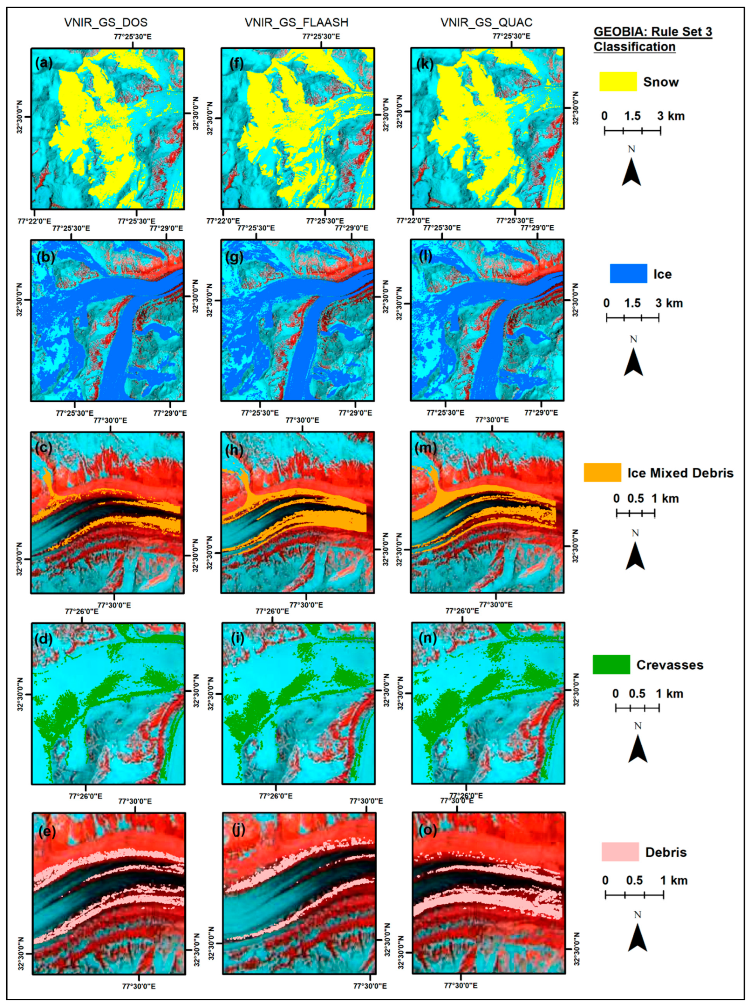
4.2. Geographic Object-Based Image Analysis

We first present the GEOBIA classification results of all band combinations across processing schemes using the F1 score as the harmonic mean of recall and precision. The performance of the classifiers is presented as an average across both study areas and processing schemes in

Table 9. Performance of GEOBIA in the current study averaged across all processing schemes for each subset using the F1 score. The values of the best performing classifiers are highlighted in bold and italicized.

Rule Sets	Spectral Band Combinations				Average
	BGRN1	CYRN2	VNIR	VNIR_SWIR
Rule Set 1	0.75	0.73	0.77	0.73	0.75
Rule Set 2	0.73	0.72	0.75	0.72	0.73
Rule Set 3	0.86	0.85	0.86	0.85	0.85

. Rule Set 3 achieved the highest F1 score across all image subsets, followed by rule set 1 and lastly rule set 2. Thus, the performance of the spectral band combinations is ranked as follows: BGRN1 = VNIR > VNIR_SWIR = CYRN2.

4.2.1. Effect of Atmospheric Corrections on GEOBIA

The effect of atmospheric correction algorithms on the GEOBIA classifications of facies using each band combination is presented here as an average of both study areas. The OA is used here as a comparative measure.

Table 10. Performance of the GEOBIA rule sets according to each atmospheric correction across all image subsets using OA as the evaluative measure. The values of the best performing classifiers are highlighted in bold and italicized.

Classifier	Comparison between Atmospheric Corrections Using Overall Accuracy
	BGRN1			CYRN2			VNIR			VNIR_SWIR
	DOS	FLAASH	QUAC	DOS	FLAASH	QUAC	DOS	FLAASH	QUAC	DOS	FLAASH	QUAC
Rule Set 1	0.73	0.81	0.77	0.72	0.79	0.76	0.77	0.81	0.78	0.72	0.79	0.76
Rule Set 2	0.83	0.75	0.84	0.82	0.76	0.83	0.85	0.77	0.84	0.82	0.76	0.83
Rule Set 3	0.87	0.84	0.87	0.86	0.84	0.87	0.87	0.84	0.87	0.86	0.84	0.87

displays the OA for all GEOBIA classifiers across each image subset based on atmospheric corrections.

For all subsets, rule set 3 delivered the maximum OA. For the DOS and QUAC classifications, rule set 1 delivered the lowest OA, whereas, for the FLAASH classifications, rule set 2 yielded the minimum OA. The trend of rule set reliability for DOS and QUAC is rule set 3 > rule set 2 > rule set 1. The trend of rule set reliability for FLAASH is rule set 3 > rule set 1 > rule set 2. For the image subsets, the reliability of atmospheric corrections is QUAC > DOS > FLAASH.

4.2.2. Effect of Pansharpening on GEOBIA

The effect of pansharpening algorithms on the GEOBIA classifications of facies using each band combination is presented here as an average of both study areas. The ER is used here as a comparative measure.

Table 11. Effect of Pansharpening across each image subset based on average error rate. NP: Not pansharpened, GS: Gram–Schmidt, HCS: Hyperspherical Color Sharpening. All the values are calculated as averages across the atmospheric corrections.

Classifier	Comparison between Pansharpening Methods Using Error Rate
	BGRN1			CYRN2			VNIR				VNIR_SWIR
	NP	GS	HCS	NP	GS	HCS	NP	GS	HCS	NP	GS	HCS
Rule Set 1	0.24	0.24	0.24	0.25	0.24	0.26	0.25	0.24	0.23	0.25	0.24	0.26
Rule Set 2	0.20	0.26	0.33	0.20	0.27	0.35	0.20	0.25	0.32	0.20	0.27	0.35
Rule Set 3	0.15	0.14	0.16	0.15	0.14	0.15	0.15	0.14	0.14	0.15	0.14	0.15

displays the ER for all GEOBIA classifiers across each image subset based on methods of pansharpening.

Among the BGRN1 subsets, GS and HCS deliver cumulative ERs of 0.24 for rule set 1. For rule set 2, GS and HCS deliver ERs of 0.26 and 0.33, respectively. For rule set 3, GS and HCS yield ERs of 0.14 and 0.16, respectively. Among the CYRN2 subsets, GS and HCS deliver ERs of 0.24 and 0.26 for rule set 1, 0.27 and 0.35 for rule set 2, and 0.14 and 0.15 for rule set 3. Among the VNIR subsets, GS and HCS deliver ERs of 0.24 and 0.23 for rule set 1, 0.25 and 0.32 for rule set 2, and a common 0.14 for rule set 3. Among the VNIR_SWIR subsets, GS delivered ERs of 0.24, 0.27, and 0.14 for rule sets 1, 2, and 3. However, HCS delivered ERs of 0.26, 0.35, and 0.15 each for rule sets 1, 2, and 3, respectively.

Hence, averaging across rule sets, the reliability of pansharpening performance for GEOBIA in the current study is GS > HCS.

4.3. Discussion

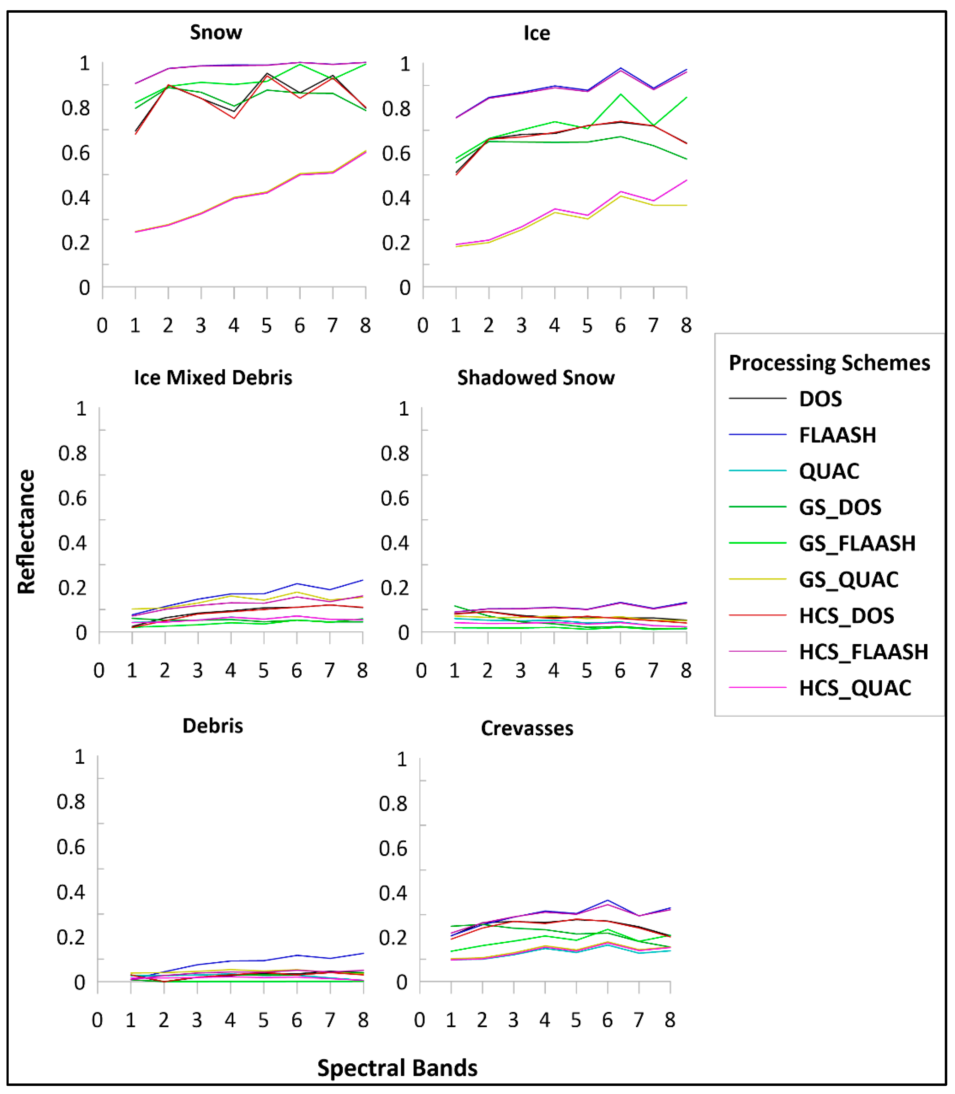
4.3.1. Manifestation of Facies

Although the total number and type of facies are discernible at the end of summer, it is the mapping method which ultimately characterizes pixels/objects to a thematic class. In Figure 5, we observe the facies of ML for the VNIR_DOS processing scheme classified by the MXL algorithm. Figure 6 highlights the mapped facies using the VNIR_DOS scheme characterized by MXL for the Samudra Tapu (ST) glacier. The highest elevation of the glacier is shadowed due to illumination conditions at the time of screen capture. In lower latitudes, higher solar elevation angle may reduce the provenance of shadow due to illumination, but the steep terrain of mountain glaciers causes shadows to be a persistent problem [64]. While some facies such as wet snow, melting snow, and saturated snow can be visually identified within the shadowed area due to varying intensity of the shadow, the same classes provide complex spectral properties within the overall shadowed area. This adds to the difficulty in isolating specific classes within shadows. Hence, the entire shadowed area is termed as shadowed snow as many of the different snow classes are encompassed within it (Paper 2). Distribution of facies follows the natural accumulation and ablation cycle with dry snow at the highest elevation, followed by wet snow, and melting snow. Similarly, the ablation region is characterized by glacier ice, melting glacier ice, dirty ice, and streams and crevasses. Saturated snow is an interesting class in the current study which is the transition facies between accumulation and ablation. This is classified here as a ‘snow’ class.

Garg et al. [65] utilized end of ablation SAR data to map dry snow, wet snow/middle percolation, percolation refreeze, superimposed ice, and clean ice zones for the same glaciers in Ny-Ålesund. The authors utilized the boundary between wet snow and clean ice to delineate the ELA. In the current study, the region characterized by Garg et al. [65] as wet snow is further differentiated into wet snow and melting snow based on reduced reflectance [10]. Moreover, dry snow was not identified using SAR on the same glaciers [65]. VHR optical sensors may have an advantage here as dry snow in the present study is found limited to the highest elevation and could be characterized based on its maximum reflectance indicative of no infiltration of water Paper 1, [66]. Dry snow is bright and therefore highly reflective [7]. Visual identification of dry and wet snow can be made based on the reduction in reflectance and slightly darker appearance (Paper 1). Spectral variations highlight the drop in intensity of reflectance of wet snow when compared to dry snow in all processing schemes (Figure 3). This indicates a broad separability of dry snow with all processing schemes. In the current study, dry and wet snow are part of several facies on the glaciers in Ny-Ålesund. However, depending on the method of mapping and broad goal of the study, the context and definition of wet snow appear to be different. This also stems from the purpose of snow-covered area (SCA) mapping, which is typically performed for large regions and considers the entire glacier as ‘snow’ and is not necessarily focused on identifying facies (Paper 2).

For example, Snapir et al. [67] combined MODIS SCA maps with Sentinel-1 composites to distinguish between dry and wet snow for two large reservoir catchments in the Himalayas with a total area of 55,000 km². In such a case, the purpose of wet snow detection is to supplement monitoring of snowmelt and improve watershed management. Moreover, the authors found that SAR underestimates wet snow when the pixel contains a mix of dry and wet snow near the snow line. VHR optical sensors can improve discrimination of these classes due to fine resolution, if accompanied by the appropriate mapping method. Karbou et al. [68] compared Sentinel-1 wet snow extent and Sentinel-2 snow products for a temporal analysis to assist determination of melt-out. Over glacier areas, Sentinel-1 displayed an underestimation of wet snow extent. Although this underestimation is partially due to geometric distortions and differences in sensor properties, it may indicate toward greater applicability of optical sensors for wet snow extent over glacier areas. Nagajothi et al. [69] mapped dry snow, wet snow, and moraine covered ice using Sentinel 2A images for the Miyar glacier. The distinction between dry and wet snow was performed using an NIR threshold. Interestingly, the authors highlighted that wet snow and glacial ice have similar reflectance properties and can be distinguished on optical images through the shape and occurrence. In the current study, we also observe similar reflectance patterns between ice and wet snow (Figure 3). However, both PBIA and GEOBIA were able to differentiate between the two classes without misclassification. While in GEOBIA the customized ratios and manual thresholding is the cause for successful mapping, PBIA seems effective in differentiating these classes too. However, it is important to note that this is true only for the MXL and WTA classification using VNIR_DOS without any pansharpening. GEOBIA is clearly more accurate (Section 4.2.); however, PBIA can be effective if the image processing and mapping methods are selected carefully. Recently, Yousuf et al. [70] mapped wet snow along with other available facies using AWiFS and Sentinel-2A. The authors utilized ancillary data such as elevation, band ratios, and variances derived from principal components to perform sub-pixel classification using a pair wise classification strategy in a support vector machine (SVM). Sub-pixel classification in this case was accomplished by blending the pixels of higher resolution Sentinel-2A imagery with coarser resolution AWiFS data. The spatial resolution of the current imagery is 0.31 m at its finest (pansharpened WV-3). Hard pixel supervised classification in the current study was capable of mapping all the facies without ancillary data. However, GEOBIA rule sets in the current study are defined based on various object features described in Table 5. These objects were formed based on aggregation of homogenous pixels using multiresolution segmentation. Currently, these object features used cannot be considered as ancillary data as they are products solely created from the object properties themselves. Hence, the current study using both PBIA and GEOBIA was able to map glacier facies across different spectral band combinations, with VNIR achieving the highest accuracy.

Melting snow is a surface facies not usually mapped in the broad characterization of glacier facies. Often, melting snow is either monitored as wet snow in the mapping of dry and wet snow to simplify facies characterization for purposes such as snow cover mapping [71] and seasonal melt coupled with precipitation runoff dynamics [72] or it is considered to be glacial melt with the objective of overall glacial discharge modelling via SCA and watershed modelling [73]. From this, it is possible to surmise that snowmelt (run-off) is distinct from the melting snow surface facies in that it is the sum release of water from the melting of snow/ice and its transport via supraglacial streams and englacial and/or subglacial channels. Liang et al. [74] mapped melting surfaces on the Antarctic Ice sheet while monitoring freeze-thaw dynamics using time series analysis via Google Earth Engine (GEE) and Sentinel-1 SAR. The authors used this to observe spatiotemporal changes in surface melt activity. The facies mapped were dry snow, melting surfaces, and refrozen surfaces. Drops in the intensity of backscatter echo during summer were used to detect presence of liquid in the snow. In the broad context of freeze-thaw dynamics, penetration of water in the snowpack can be characterized generally as a melting surface/wet snow. However, in the specific context of glacier facies, wet snow and melting snow may be different surface facies based on the reduction in reflectance, elevation, and visible properties. Facies are individualistic to glaciers and some facies may exist on some but not on others. In this study, we are focused on identifying the maximum range of facies and testing the variability in the final thematic by modulating the image processing and mapping method. Hence, while it is possible to merge wet snow and melting snow, the utility of conventional PBIA with VHR VNIR data to track subtle variations in facies is key for robust mapping operations. GEOBIA is most accurate, but PBIA is more efficient. Mendes Jr. et al. [75] mapped glacier radar facies in Antarctica to retrieve snowmelt by monitoring the wet snow zone. The authors also mapped dry snow, frozen percolation, and bare ice zones. The authors highlighted that radar zones/facies are based on the surface properties of glacial bodies, whereas classical/glaciological facies depend on the properties of the entire glacier due to the previous accumulation [76]. Pope and Rees [16] highlighted the same with optical facies suggesting that optical mapping of facies can be surface classes rather than glaciological facies. Nonetheless, at the end of ablation season, when most of the seasonal now has melted, the maximum variations of facies are discernible. Unless a sudden precipitation event occurs prior to the date of image capture, the occurrence of facies should not differ. We found no recorded precipitation event before the date of image acquisition in the current study (Paper 1). However, without in situ monitoring of the subsurface phenomena, a direct and accurate characterization of glacier facies is not advisable. Due to this, in our previous work [3], we utilized the name surface facies to refer to the end of ablation facies mapped by optical imagery. In the current study, melting snow differed from wet snow in that it exhibited lower reflectance and is showed higher reflectance than saturated snow (Paper 1 and Figure 3). This slight variation is only effectively characterized by the reflectance obtained from VNIR_DOS and VNIR_FLAASH image subsets. This suggests that pansharpening does not enhance separability of closely matching but distinct surface facies. Moreover, the higher accuracy of MXL and WTA suggest that only in the combination of VNIR_DOS/FLAASH and either MXL or WTA can PBIA accurately map these facies. GEOBIA rule set 3 overcomes the effects of image processing and in fact improves after pansharpening. However, rule sets are analyst driven. The development of each rule set permits a detailed evaluation of objects, object features, and the individual exertions of each feature for each facies. This will lead to a highly accurate thematic map, but it is achieved at the expense of efficiency. However, the saturated snow class presents an interesting case because, if the ELA was characterized previously using the border between wet snow and clean ice [65], in the present case, it would be the border between melting snow and saturated snow. Pope and Rees [16] found two snow classes on the ML glacier using unsupervised classification of Landsat ETM+ imagery. The extent of snow class 6 identified by Pope and Rees [16] is similar to the saturated snow extent identified here. Moreover, the facies was named saturated snow as its reflectance resembled that of the same class identified by Hinkler et al. [77]. All the facies are characterized by observing similar reflectance properties with previous literature (Paper 1).

The ice facies in the current study correspond to glacial ice occurring below the ELA for the respective glaciers. Glacial ice is generally ‘clean’ with ice mixed with debris or dirty ice being characterized separately. While in SCA mapping ice and snow facies may often be considered into the overall glacier body, in facies mapping, they are usually categorized independently. Bhardwaj et al. [6] aggregated ice and snow into one class considering it as the accumulation region while mapping supraglacial debris and ice mixed debris on two small glaciers in the Chandra-Bhaga basin. The mapping was performed using band ratios of Landsat TM and ETM+ images, utilizing an ASTER DEM for deriving slope and curvature. Due to the coarser resolution of Landsat ETM+ images, slope and curvature derived from the DEM was necessary to delineate glacier boundaries. In the current study, VHR images visualized as 3D surfaces with base heights derived from the ASTER GDEM v2 were efficient in identifying all the glacier boundaries in Ny-Ålesund, as well as some of the ice divides in the Chandra-Bhaga basin [3]. Moreover, the greater range of accumulation and ablation surface facies are discernible using VHR VNIR_SWIR data. Bhardwaj et al. [56] mapped snow and clean ice independently in addition to slush, crevasses, dirty ice, and supraglacial debris using Landsat 8 OLI. Interestingly, the authors utilized TOA reflectance and brightness temperature. Atmospheric correction algorithms convert TOA reflectance to apparent surface reflectance, thereby providing a comparison against established spectral signatures of identified facies. This allowed for a comparison with the spectral characteristics of ice in this study against previous extractions of spectral reflectance for the same facies (3, Paper 1). Moreover, when compared against different image processing methods, the VNIR_DOS stands out as the most reliable. The spectral reflectance pattern of ice in the current study resembles that from Prieur et al. [78] extracted using Landsat 8 OLI. Keshri et al. [5] distinguished snow and ice after separating debris and ice mixed debris utilizing a stepwise implementation of Normalized Difference Snow Index (NDSI), Normalized Difference Glacier Index (NGDI), and Normalized Difference Snow Ice Index (NDSII). This approach is similar in implementation to GEOBIA rule sets. GEOBIA rule sets are formed after a careful evaluation of object features and customized features followed by a stepwise assignment of thresholds, and categorization into thematic classes. In Paper 2, we provided all the rule sets used for mapping. For example, in Ny-Ålesund, in all the rule sets, ice is classified at the end after all the other facies are extracted. Only rule set 2, for the VNIR_DOS subset, necessitated that ice be classified before melting glacier ice using the min. pixel value of the red edge band. In the case of rule set 1 for VNIR_FLAASH, ice was mapped using the mean reflectance of the coastal band. In rule set 3, using the VNIR_QUAC, ice was mapped using the min. pixel value of the green band. For the Chandra-Bhaga basin, using rule set 1 for the HCS_FLAASH, ice was mapped using the mean reflectance of the NIR band. In rule set 2 using the HCS_QUAC subset, ice was characterized using the quantile of the green band. In rule set 3, using HCS_FLAASH, ice was categorized using the mean reflectance of NIR2 and the quantile of the coastal band. All facies are characterizable using each of the spectral band combinations and each image processing scheme. VNIR is most accurate, however, GEOBIA permits mapping due to the intervention of an analyst molding the rule sets according to the image processing scheme. Nonetheless, even PBIA via MXL is capable of mapping ice. Azoni et al. [79] mapped ice using the MXL algorithm on the Forni glacier using VHR UAV orthophotos (0.15 m spatial resolution) with a high precision of 0.91. The order of facies characterization is important as outlined by the procedure adopted by Keshri et al. [5]. This process, though time consuming and not as straight forward as supervised PBIA, is effective in exploiting the limitations introduced by limited spectral bands. Alifu et al. [80] utilized a TIR/NIR/SWIR band ratio to map supraglacial debris by separating the rest of the glacier as clean ice using a density slice approach. The authors also utilized a similar geomorphometric approach as Bhardwaj et al. [6] to separate the glacier from the non-glacier area. In the current study, however, ice was mappable without the use of thermal bands in the satellite imagery, by simple PBIA and by mean reflectance and object features in GEOBIA. In a machine learning-based classification of glacier surface classes, MXL, SVM, and RF classifiers were tested using a combination of Landsat TM and OLI with a range of normalized difference indices to support the characterization [81]. All three methods delivered greater than 99% accuracy, with the SVM only slightly outperforming the other methods. Although the facies themselves were limited to three, the performance of the MXL is attributed to its robust capacity [82].

The dirty ice and alluvial/depositional fan conjunction is important for accurately mapping glacier extents. Dirty ice in the current study was characterized previously as off-glacier [16]. The current imagery highlights water bodies outside the glacial terminus in the alluvial fan (Figure 5). Manual digitization of the glacier terminus using the 3D elevation surface (upper left inset, Figure 5) aided in avoiding possible confusion between the alluvial/depositional fan and dirty ice. Dirty ice is also important because this facies is suggested to have a higher melt rate than other facies [83]. Dirty ice is defined as partially debris-covered ice [83,84]. The Ostrem curve suggests that debris cover lesser than the ‘critical thickness’ of debris increases melt [85,86]. Moreover, areas with thin and partial debris cover are discontinuous [83] leading to difficulty in effective mapping. Mapping of patchy and thin debris cover is necessary to track spatial variations in ablation. VHR optical sensors may enable efficient mapping of dirty ice by improved visibility due to enhanced spatial resolution (Paper 1) and tracking of reflectance variability due to sensitivity in the NIR region [16]. Accurate mapping of dirty ice would improve spatially distributed ablation modeling. In the current study, digitization of the glacier supported by 3D surface analysis enabled accurate extraction of the glacier body. Dirty ice is also observed in the upper regions of the glacier (Figure 5) intermixed with saturated snow and streams and crevasses. This may be attributed to misclassification of streams and crevasses into dirty ice due to some spectral overlap in the visible range (Figure 3). While temporal analysis movement of debris may permit a detailed explanation of the occurrence of dirty ice at higher elevations, it is beyond the scope of the current study. The intermixing of saturated snow, streams, and crevasses and dirty ice may be explained by the emergence of debris from fine transverse crevasses which are then dislodged by melt and supraglacial streams and transported into the dirty ice region [83]. The occurrence of dirty ice at the edges of the glacier may be due to the entrainment of debris and dirt along its margins [87,88]. Haq et al. [87] mapped dirty ice using Hyperion hyperspectral data and Random Forest classification in the Indian Himalayas. In the spectral reflectance drawn from Hyperion imagery, dirty ice shows maximum spectral separability in the visible range. Between 750–800 nm, dirty ice shows an overlap with ice mixed debris, after which the SWIR range contains minimal variations between all facies [87]. Thus, in the absence of hyperspectral imagery, VHR VNIR imagery may hold a key advantage for mapping patchy and discontinuous debris cover. In the current study, the VNIR subset yielded better performance among all atmospheric corrections and pansharpening methods. Florath et al. [89] (2022) mapped a range of facies including dirty ice in a comparative assessment of unsupervised and supervised classification methods. Their results highlight the efficacy of supervised approaches such as Random Forest (RF) in mapping facies. However, their results were based on mapping carried out on Sentinel-2A images. In the current study, we evaluated several spectral band combinations and found that the best mapping of not only dirty ice, but all facies was without the SWIR range. Hence, the VNIR spectrum still holds maximum potential for executing PBIA and GEOBIA spatial-spectral approaches for mapping patchy debris. However, both Florath et al. [89] and the current study highlight the utility of supervised approaches for mapping glacier facies when ancillary data are not available. Separability of spectral signatures is key for identification and mapping of facies. Dirty ice can be confusing because of the confounding spectral signatures with streams and crevasses. Advanced classification methods are poor at generalizing spectral signatures into constituent classes (Paper 1), in such cases, simpler algorithms such as MXL and MHD may classify better. While GEOBIA rule set 3 is much more accurate than PBIA, the time needed to develop rule sets can be detrimental when faster albeit slightly less accurate methods can be utilized.

Ice mixed debris (IMD) is a mixture of debris of varying sizes with ice [87,90]. Spectrally, it is of slightly higher reflectance than debris [3] and lower reflectance than ice [91] and is most prevalent in the ablation zone. Accurate mapping of IMD like dirty ice and debris is important because the conversion of IMD to debris can be a direct assessment of the impact of climatic variations on the health of the glacier [92]. A reliance on thermal bands to isolate ice mixed debris and debris from the overall glacier body is well reported in literature [5,70,92,93,94]. In the current study, we lack thermal bands in the sensor. Moreover, as the present focus is on mapping facies without the ancillary inputs from other datasets, we have relied purely on the visual and spectral properties of the facies arising from the imagery and previous literature to guide the classification strategy. The spectral signatures of IMD arising from DOS and FLAASH corrections are most useful for comparative purposes and have a better contrast against debris. This is most important for PBIA as only non-pansharpened subsets led to accurate extraction by MXL. However, GEOBIA overcomes the distortions in spectral signatures induced by all image processing schemes. In the absence of thermal bands, elevation-based information derived from DEMs, band ratioing, and/or spectral indices are necessary for mapping IMD [95]. In a comparative assessment of a hierarchical knowledge-based classification (HKBC) utilizing ancillary information from DEMs, ratios, and indices against MXL, the HKBC classified IMD better with a user’s accuracy of 81.82% [91]. Parallels against the current study can be drawn by considering the superior performance of GEOBIA against PBIA. However, we have only utilized image data to generate objects and their features. Rule sets themselves are knowledge-driven on account of stepwise development. Even sub-pixel mapping of IMD utilizing SVM has relied on ancillary information from both DEMs and thermal bands when using medium-to-high resolution imagery [70]. Our results point toward the efficacy of VHR imagery in congruence with appropriate mapping methods for effective characterization of debris. Extraction of IMD or debris via hyperspectral images require significant preprocessing for removal of noise, bad bands, segregation of pure spectra, and atmospheric correction. Although such extensive processing yields accurate results, it is time consuming [87]. In such cases, the current study may prove useful as the lack of spectral bands may be overcome by utilizing VHR data and spatial-spectral GEOBIA rule sets. In a recent GEOBIA based approach for mapping debris cover in addition to other facies, Mitkari et al. [22] utilized thermal infrared (TIR) band (Landsat TM) and a NIR2/Yellow index (Table 5) from WV-2 to map IMD. In the current study, we have also utilized the same index for mapping IMD for the CYRN2, VNIR, and VNIR_SWIR rule set 1 and 3 subsets. However, for the BGRN1, the R_B index (Table 5) was sufficient but not ideal. For rule set 2, IMD was characterized using the max. pixel value of the objects in the green band. The average threshold range for this was 0.05–0.15 (Paper 2). However, this value changed based on atmospheric correction and pansharpening.

Supraglacial debris cover occurs by the entrainment and deposition of bedrock material in the ablation zone due to the interplay of summer ablation and the glacier’s movement. Based on the size, deposition, and intermixing with ice, the surface facies may transition from dirty ice, to IMD, to debris cover with ice now beneath a continuous debris cover. Other sources of debris input consist of rockfalls and mass movements from the surrounding valley, as well as deposition via strong winds. Debris-covered glaciers are defined as a glacier, wherein a portion of the ablation region is overlain by a continuous cover of debris across its width [96,97]. The varying influence of the spatiotemporal dimensions of debris on the ablation of the glacier has been the core of several investigations [83,92,96,98,99,100,101]. In the current study, we observed the debris class only on the Chandra-Bhaga Basin glaciers as the Himalayas are known to possess a cover of debris in the ablation zone [97,102]. Glaciers in Ny-Ålesund are known to be relatively clean [7]; therefore, the facies at the end of the ablation zone was characterized as dirty ice. Pratibha and Kulkarni [99] mapped temporal changes in supraglacial debris by first classifying snow and snow-free areas of the glaciers using MXL, and subsequently applying band ratios derived from Landsat OLI, ETM, and TM imagery to characterize debris. Although the study did not utilize thermal bands, it relied upon images of three different Landsat sensors to successfully map debris. Nonetheless, it does highlight the utility of simple processing methods to extract debris cover. Mölg et al. [64] created an inventory of the debris cover in High Mountain Asia using a threshold on band ratios on Landsat TM and ETM+ imagery. However, Azzoni et al. [79] suggest that debris mapping is more reliable via VHR imagery because of the capacity to distinguish between debris cover of various distributions, and smaller features such as cones which may be misclassified in coarser resolution data. Kaushik et al. [103] utilized a deep neural network (DNN) to map debris with a combination of optical, SAR, and elevation data. The authors trained the DNN framework over different test sites in the Himalayas and then applied it to a different region. This highlights the potential transferability of the authors’ method. However, this DNN structure can misclassify IMD or dirty ice into debris class as the method is not trained for a range of facies, but rather specifically for variations in supraglacial debris of different glaciers. Robson et al. [9] combined optical, SAR coherence, and elevation data in a GEOBIA domain to distinguish clean ice, glacial lakes, and debris. The authors utilized a three-step hierarchical segmentation approach to separate the classes. In the current study, the same multiresolution segmentation parameters were applicable for mapping debris in all the different processing schemes (Paper 2). In a GEOBIA based mapping of supraglacial debris in Antarctica using WV-2 imagery, debris was mapped with an overall accuracy of 93% [104]. However, the authors noted that the geomorphology of Antarctica induces spectral similarity between many of the features. In the current study, the spectral contrast between debris, snow, ice, and crevasses is quite large. The separability with IMD is appreciable, with shadowed snow being the most confusing class. This may highlight why PBIA using MXL here provided better results than that observed in Antarctica (Paper 1, [104]). We extracted debris using the max. pixel value of NIR1/2 for rule sets 2 and 3, the R_B ratio for BGRN1 and the mean reflectance of NIR2 for VNIR and VNIR_SWIR in rule sets 1 and 3. Mitkari et al. [22] utilized brightness temperature and slope via GEOBIA to separate supraglacial and periglacial debris. Often, boundaries of debris-covered glaciers are difficult to ascertain without the use of ancillary data due to confounding properties with the surrounding geology. Manual delineation of glacier boundaries is therefore a practical approach to ascertain minimal error of misclassification [3,56,99].

Crevasses are elongated deep cracks or fractures in the ice [22] resulting from the type of flow of the glacier [105]. Owing to this shape, crevasses may be easily detected in GEOBIA via the appropriate segmentation parameter. The spectral signature of a crevasse is usually of lower intensity than ice but maintains the same trend [3]. This can lead to misclassification of crevasses. Although crevasses are not considered as classical/glaciological facies, they are important surface facies due to their hazard potential. As crevasses represent the dynamicity of the glacier, identifying their extent and shape is useful for understanding mass balance processes [106]. In the Chandra-Bhaga basin, we observe that the crevasses are clearly discernible and mostly benefit from GEOBIA GS_QUAC_VNIR_Rule sets 2 and 3. This is because rule set 2 utilizes mostly spatial and contextual information, wherein the standard deviation object feature of the Yellow (CYRN2/VNIR/VNIR_SWIR subsets) and NIR1/2 (BGRN1/VNIR VNIR/VNIR_SWIR subsets) were applied successfully. The same features were utilized in rule set 3 as it combines both spatial and spectral information. In rule set 1, where only direct spectral information was used, the R_RE, N2_Y, and mean reflectance of the red band (Table 5) ratios were used to delineate crevasses. In Ny-Ålesund, streams and crevasses were categorized into one class, as the width of these facies is much smaller than that of the Chandra-Bhaga Basin crevasses. Moreover, supraglacial streams transport water via crevasse channels and categorizing them into one facies helped in ensuring spectral separability of the other facies. Moreover, the disheveled appearance of crevasses in Chandra-Bhaga Basin aided in their visual identification alongside enhancing the contextual capabilities of GEOBIA. A U-Net-based deep-learning model for mapping crevasses and supraglacial streams highlighted the necessity of mapping fine stripe crevasses which are only visible at fine spatial resolutions [107]. The VHR GEOBIA method employed here can be used to supplement Ground Penetrating Radar (GPR) based investigations of crevasses [108,109] to highlight risky zones.

4.3.2. Variations in the Best Performance

The striking factor of the segmentation parameters used here is the wide applicability across all the image processing methods for both study areas. This contradicts the assertions by Hao et al. [110], who suggest that because objects generated in VHR imagery are molded by a larger number of pixels [111] and different image targets will require different scale parameters. This supports the necessity of multiscale segmentation for different image targets. However, the authors [110] also observed that the image objects’ size/area is affected by more factors than just the scale parameter. These factors include spectral, spatial, and geometric properties. Multiresolution segmentation permits the analyst to exert greater control over the resultant objects by modulating the segmentation criteria [112]. This causes the determination of ‘optimal’ segmentation parameters to be subjective, time-consuming, and challenging [113]. Built up areas with buildings offers crisp geometric shapes clearly discernible in VHR imagery which can be useful for extracting these features. However, natural land covers may often have image targets with close spectral and spatial properties. Multiscale image segmentation has been employed to map glacier cirques [114], volcanic landforms [115], Antarctic supraglacial debris [104], glacier facies [9,22], and glacial landforms [116]. However, single scale segmentation has also proven useful in delineating objects for mapping landslide-dammed lakes [117], snow cover [118], supraglacial ponds [119], and icebergs [120]. Ice marginal lakes were extracted using two different segmentation parameters for Sentinel-1 and Sentinel-2 imagery [121]. Although it is not an optical vs. optical image comparison, the same lakes required two different scales with two different sensors. Spatiotemporal analysis of forest cover found that pixels in Corona and Landsat TM/OLI imagery can be segmented using similar scale parameters [122]. This highlights that both single and multiscale parameters can be effectively utilized for segmenting objects of varying sizes. According to our knowledge, no study has evaluated the impact of image processing routines on the resultant characterization of glacier surface facies using GEOBIA or PBIA. This is significant because the selection of the basic process to derive reflectance introduces changes in the spectral signatures of image targets. Moreover, pansharpening increases the number of pixels aggregated into objects. Therefore, the necessity to evaluate modulations needed for subsets of each processing scheme in segmentation and rule set development is non-trivial. In the current study, we find that no change in scale parameter is needed when segmenting any of the various subsets. This suggests that the parameters applied here may be transferred to other VHR imagery for segmenting glacier surfaces. However, every subset required individual manual modulations to test the applicable ratios/features, the thresholds for each feature, and the order of extracting facies. Multiscale segmentation utilizes different object sizes to match different image targets. It follows the logic that object features may have overlapping properties for various facies. This is extended to rule sets as well because, even if a single segmentation level was sufficient to delineate objects for all image targets, object features must be evaluated and extracted individually. As each processing scheme modifies the spectral properties of the pixels in those subsets (Figure 3 and Figure 4), rule sets utilizing features based on spectral properties will require reconfiguration. This extends to pansharpened subsets as well because GS and HCS also exert differential impacts on the overall spectral and spatial quality of the image. Each rule set was created methodically after segmenting based on step-by-step observations for individual subsets. Thus, GEOBIA rule set 3 delivers high accuracy and robust effectivity but is exhaustive in applicability.

The technical calculations described in Section 4.2. highlight the high accuracies obtained by GEOBIA rule set 3. The modifications in this rule set for each processing scheme also resulted in changes in the final thematic maps. Figure 7 highlights the differences in mapped facies on the Samudra Tapu glacier from rule set 3 for the VNIR_GS_DOS, VNIR_GS_FLAASH, and VNIR_GS_QUAC subsets, respectively. GS_FLAASH overestimates snow in the ablation region but simultaneously shows a patchy distribution in the well-known accumulation area [123], whereas GS_DOS only slightly underestimates snow in the accumulation zone. Both GS_DOS and GS_FLAASH overestimate ice in the accumulation zone due to the misclassification of some areas into ice. GS_ QUAC yields a better overall coverage of snow and ice. The classification of debris from the GS_QUAC subset closely follows the known occurrence of the same facies [94]. However, GS_DOS underestimates and GS_FLAASH overestimates debris when compared with GS_QUAC. Crevasses are well mapped by all three processing schemes, highlighting the efficacy of GEOBIA in extracting these minor features. IMD shows a large variability between all three subsets. GS_QUAC appears to have characterized IMD more efficiently against the overestimation by GS_FLAASH and underestimation by GS_QUAC. In recent years, the overall glacier area in the Chandra-Bhaga Basin is found to be larger than other basins in the Himalayas [124]. This is attributed to the higher elevation of this basin and the reduction in wet precipitation with dry precipitation being consistent [124]. The month and year of image acquisition in the Chandra-Basin is reported to have a larger distribution of SCA [124,125]. Thus, distribution of snow and ice in the current imagery (Figure 7) observed from the GS_QUAC subset is consistent with recent findings. These variations are important because selection of the most appropriate image processing routine for any imagery would ideally yield the most realistic and accurate thematic classification. This is also evident from the fact that in PBIA pansharpening reduced the performance, whereas, in GEOBIA, it enhanced the result. To the best of our knowledge, no other study has compared the impact of variations in image processing in GEOBIA for mapping facies; this makes a direct comparison with the current results difficult.

4.4. Comparative Analysis

In this study, we have attempted to compile the results of Paper 1 and Paper 2 with additions of the variations of spectral band combinations into the processing routine based GEOBIA and PBIA analysis of glacier surface facies.

It is observed that the literature for selection of atmospheric correction and pansharpening algorithms described in Paper 1 often delivers a recommendation that is application specific [25]. The addition of SWIR bands to the classification in both PBIA and OBIA did not significantly enhance the results. For pixel-based classification, it was found that the bands most affected by atmospheric effects (Coastal and Blue) were the main bands used to decipher atmospheric information [126,127]. Moreover, NIR 1 and NIR 2 are strongly influenced by water absorption and dispersion of suspended particles [128]. The FLAASH algorithm which utilizes these bands to predict the atmospheric effects would then be most affected by detrimental effects of pansharpening on the spectral information (Paper 1). In PBIA based on VNIR data (Paper 1), it was found that the FLAASH atmospheric correction performed better. However, when tested across various spectral band combinations in PBIA, the DOS correction yields superior rigor. This implies that the DOS may be more suitable for large data volume analysis using PBIA. Furthermore, as the DOS algorithm is simplistic in its configuration Paper 1 [129], it may promote faster analysis. In the GEOBIA domain, however, the QUAC algorithm delivered superior results. Karimi et al. [31] mapped debris covered glaciers using the QUAC algorithm as the image correction method with efficient results. In the current case, this study is the first of its kind to test image correction methods for the application of glacier surface facies. The FLAASH correction generally delivers the most realistic spectral reflectance [130,131] and is consistent using VNIR imagery. However, across image processing mechanisms, we find it delivers inferior results when compared to DOS and QUAC.

The nature of classification algorithm and workflows sometimes necessitate specification of Red, Blue, Green, and NIR bands. For example, the TERCAT workflow in ENVI requires this information before proceeding to classification. It would make intuitive sense that substitution of these bands by manipulating spectral band subsets will result in variations in classification using the same image. Here we find that the VNIR and BGRN1 subsets deliver superior results when compared to CYRN2 and VNIR_SWIR. This is true for both PBIA and GEOBIA processes. While GEOBIA delivers superior performance across all atmospheric corrections and pansharpening methods, it appears that conventional spectral bands retain maximum capacity for targeted information extraction. SWIR bands can aid in the mapping of glacier debris and even help define ratios for mapping dust and supraglacial mineral composition [132]. This was found to be true for the GEOBIA rule sets. SWIR bands were most useful in the delineation of dirty ice. However, object features based on VNIR imagery were also capable for mapping dirty ice. Moreover, the image subsets with the best GEOBIA based mapping in the current study are BGRN1 and VNIR; this may again point towards the utility of conventional spectral bands for mapping facies. Moreover, as this mapping can be accomplished without SWIR, the focus on VNIR data for mapping glacier facies and supraglacial debris can be further explored. GEOBIA across all image subsets did not require a change in the segmentation parameters of scale parameter, shape, and size. In comparison to Paper 2, much of the rule set logic is maintained. We were able to map fine features that have proven difficult in the past [133].

As observed in Paper 1, PBIA greatly suffers from the detrimental effects of pansharpening. However, we also find that MTTCIMF and TCIMF observe a modest increase in overall accuracy consistent across both pansharpening methods and image subsets. Even though this increase does not improve the overall reliability, it still points towards the possibility of improving MTTCIMF based mapping at finer resolution (Paper 1). GEOBIA, however, improves with pansharpening, with the GS delivering better results than the HCS (Paper 2). When tested across large datasets, the suitability of GS may hold true [55].

Comparative Analysis of WV-2/3 Spectral Performance

WV-3 imagery has been termed as super-spectral [134] and hyper-spatial [135]. The spectral characteristics of both WV-2 and WV-3 have been tested across many applications. Some of the main applications are agriculture (crop yield, crop productivity, crop type), mineral mapping, cryosphere (glacial lakes, glacier facies, snow cover extent), urban material characterization, flood monitoring, disaster analysis, biomass estimation, etc. Here, we discuss previous literature and then compare our own results to infer cross-application robustness (if any) of the spectral bands.

In an analysis of WV-2 for mapping specific minerals, FLAASH corrected SWIR bands were found to be most useful for alteration and hydrocarbon detection using SVM [136]. Ye at al. [136] found that the most characterizable absorption features were found in the SWIR region. Sun et al. [137] distinguished between hydroxyl, Al-OH, Mg-OH, Fe-OH, iron stained, carbonates, kaolinites, calcites, siderite, and jarosite alterations using a combination of PCA, mineral indices and SAM classification on WV-3 imagery. Their indices utilized SWIR 1, SWIR 3, SWIR 5, SWIR 6, SWIR 7, SWIR 8, green, and red edge bands. SWIR bands enhanced the results of petroleum (Hydrocarbons) characterization by Asadzadeh et al. [138]. Their results highlight the absence of hydrocarbon features in the VNIR bands and consequently the extreme reliance on SWIR bands. WV-3 SWIR bands are reported to possess better spatial consistency of mineralogical units [139]. Kruse et al. [140] compared pre-launch simulated WV-3 spectral bands with AVIRIS and post-launch WV-3 image data to map minerals using the MTMF classifier. Their results suggest that WV-3 performs better for calcite and muscovite than buddingtonite, kalinite, and silica. Most confusion was found in alluvial fan areas, which is a mixing zone for these minerals. Although glacier surface facies can be spectrally distinct, we find that spectral overlap does exist between facies, especially in the visible region (Figure 3 and Figure 4). However, most of the overlap is observed for facies in the Chandra-Bhaga Basin due to the large coverage of snow. This suggests that timing of image capture for end of ablation facies mapping is extremely crucial for observing all of a glacier’s available facies.

Hunt Jr. et al. [141] found spectral indices created using SWIR bands 2, 3, and 4 were superior in estimating leaf water content through WV-3 imagery, whereas SWIR 1 was not useful. In the current study, however, only SWIR 1 was useful. Eckert [142] found that WV-2 red edge and NIR bands have the highest correlation with field data for aboveground biomass estimation. Without field data presently, we cannot definitively suggest similar results. Nevertheless, looking at the accuracies, it is safe to assume that the NIR bands are most useful for mapping facies. The red edge band can be swapped by the red band without many changes to the final output. Of course, at least with GEOBIA, it depends on the rule sets defined by the operator. Sibanda et al. [143] found that the red edge spectrum improved grassland mapping accuracy by 14%. Pu et al. [144] also described the potential of the red edge band for detecting reduction in chlorophyll content. The efficacy of red edge is not replicable in the present study. While using a class-based sensor independent spectral band NDVI, Upadhyay et al. [145] found the Yellow, Red, Red Edge, NIR 1, and NIR 2 bands to be most applicable for mapping crops. Immitzer et al. [146] analyzed the conventional (BGRN1), additional bands (CYRN2), and full 8-band (VNIR) range of the WV-2 sensor for comparative classification of tree species using RF and GEOBIA. Like the manual digitization used to remove shadowed areas in the current study, Immitzer et al. [146] focused only on the sunlit portions of tree crowns. Akin to the present results, VNIR bands yielded maximum accuracy through GEOBIA, and the utility of the non-conventional bands was species specific. By and large, the conventional BGRN1 subsets delivered higher accuracies than the CYRN2 bands. Marshall et al. [147] found that additional bands do not improve spectral separability while testing the influence of additional bands (CYRN2) of WV-2 using MTMF for mapping invasive grass species. In an analysis of mangrove species and non-mangrove area classification, Heenkenda et al. [148] utilized spectral band combinations of pansharpened and non-sharpened imagery. They highlight the utility of pansharpened VNIR imagery for effective classification using GEOBIA. The authors suggest that rule sets can be easily transferred to other areas as they are made of image variables rather than set numerical values. Unfortunately, this is not consistent with glacier facies mapping. This may be because facies themselves vary across different glaciated areas and must first be robustly analyzed to determine their occurrence, followed by spectral characterization and then development of rule sets. However, we do believe that the segmentation parameters developed in Paper 2 and implemented here are robust as they have been applicable without any deviation. The rule sets themselves need to be assessed carefully as they are a logical progression of operator intuition and skill. Here, the rule sets applicable in Ny-Ålesund were not applicable in the Chandra-Bhaga Basin; moreover, the same rule sets were not even transferable across different processing schemes. This highlights the importance of accurate selection of image processing routines.

In a comparative analysis between DOS and FLAASH corrected images for bathymetry mapping, DOS delivered superior performance with the most useful bands being coastal, green, yellow, and NIR 2 [149]. Malinowski et al. [150] analyzed patterns of localized flooding using 12 different decision tree (DT) methods comprising of different PBIA and GEOBIA approaches on WV-2 imagery. DOS delivered more accurate reflectance for water than ATCOR. The authors highlight that NIR 2 is the most water sensitive band in the WV-2 arsenal. This could have potential for mapping saturated snow facies, but in the current study, we observe that all facies can be mapped by BGRN1 with better accuracies than CYRN2. Collin et al. [149] compared Hyperion and WV-3 data using spectral combinations of BGR (3 wavelengths), BGRNIR (4 wavelengths), CBGYR (5 wavelengths), BGRNIRs (8 wavelengths), and full 16 band spectrums in an Artificial Neural Network (ANN) structure for mapping coastal systems. The authors suggest that most of the over-reflecting discrepancies between the sensors are a result of the coarser resolution of Hyperion when compared to WV-3. Between the spectral subsets, however, the 16-band full spectrum subset delivered maximum accuracy for WV-3. In the current study, however, the VNIR (8 wavelength) subset delivered highest accuracy across all processing schemes and classification methods. One reason may be the little to no target information contained in the SWIR bands from SWIR 2 to SWIR 8. Only SWIR 1 could be used for delineating dirty ice, melting snow, and melting glacier ice. However, this was performed to utilize the SWIR band in the combination and not because it could not be alternated by a VNIR alternative. When matching field spectra to WV-2 bands to map asphalt roads, blue, green, red, and NIR 2 reported maximum usability [151]. Variations in roofing materials were distinguishable from the yellow band onwards using pansharpened WV-2 imagery [152].

Karimi et al. [31] mapped clean ice, periglacial debris cover, and supraglacial debris cover using 4 band WV-2 (CBGR) and Landsat-TM imagery. The authors performed an inter-sensor pansharpening by enhancing Landsat-TM using PAN WV-2 data, and QUAC was used to derive reflectance. The 4 band WV-2 imagery is reported to be effective in classifying ice due to its high reflectivity. The authors also differentiated the temperatures of shadowed areas, periglacial, and supraglacial debris using Landsat-TM. The goal of the current study is to only utilize the attributes of the optical imagery to determine the variations in output according to different processing schemes and classification methods. This allows for an independent robust analysis of the image itself in varying scenarios. Moreover, manual digitization of the glacier boundary in the current study did not necessitate distinction between peri- and supraglacial debris. Tiwari et al. [153] utilized WV-2 imagery solely for data interpretation purpose to identify features in the ablation zone of the Bara Shigri glacier to facilitate supraglacial debris mapping using ASTER thermal, GDEM, and TerraSAR-X imagery. Buhler et al. [154] identified wet snow and wind transported snow using WV-2 imagery. However, their analysis was performed on non-atmospherically corrected data. The NIR 2 band which was suggested to enable greater differentiation between snow surfaces did not individually enhance classification in the current study but aided in the differentiation between dry and wet snow (whenever available). Jawak et al. [155] extracted snow cover using a comparative analysis of 14 spectral index ratios on principle component sharpened and GS sharpened WV-2 imagery. Their spectral indices using the additional bands yellow, red edge, and NIR 2 were most significant in extracting snow cover. However, in the current study, only NIR 2 was moderately effective. Yellow and red edge did not add any significant improvement and could be easily replaced by green or red band. Gray et al. [156] highlighted an interesting application of WV-2/3 imagery for mapping green and red snow algae. The imagery was converted to reflectance using the 6S radiative transfer model. Algal distributions documented on field were used to train SAM classifier to distinguish between green, red, dirty, and clean snow. The authors highlighted that processing routines can induce biases in the final algal distributions. This is true even in the case of the current study. Modulations in spectral reflectance due to changing atmospheric corrections, resolution improvement by pansharpening, selection of classification algorithm (PBIA), and even operator skill (GEOBIA) play a large role in the final thematic classifications.

4.5. Final Inferences and Recommendations

The statistical evaluation tabulated and described in Section 4.1 and Section 4.2. is summarized and illustrated to outline our findings in Supplementary Figures S1–S4. Among atmospheric corrections (Supplementary Figure S1), we find that DOS (OA = 0.64) is the most reliable correction across all image subsets. When analyzed between PBIA and GEOBIA, DOS is preferred for PBIA, whereas QUAC is most suitable for GEOBIA. Among the PBIA classification methods, MXL and WTA work best with DOS. In GEOBIA, rule sets 2 and 3 work best with QUAC, whereas rule set 1 performs well with FLAASH. Between the spectral band combinations classified by PBIA, VNIR_DOS is the most accurate, whereas in GEOBIA, BGRN1_QUAC, VNIR_DOS, and VNIR_QUAC yielded maximum OA of 0.83. Among pansharpening methods (Supplementary Figure S2), HCS (0.64) delivers an overall better performance than GS. However, this is due to the aggregated extremely poor performance of GS in PBIA. In GEOBIA, both GS and HCS improve accuracy, with GS delivering the maximum OA of 0.79. Among the GEOBIA rule sets, rule set 3 shows the maximum improvement in accuracy with GS scoring an OA of 0.86. Among the PBIA classifiers, MHD yields the highest OA with HCS. Between the spectral band combinations, the VNIR_HCS combination is the best, but with a very low OA of 0.29. The VNIR_GS and BGRN1_GS combination via GEOBIA classification yields the maximum OA of (0.79). A comparison between GEOBIA rule sets and PBIA classifiers (Supplementary Figure S3) outlines that GEOBIA is the most accurate with rule set 3 delivering the highest OA of 0.86. Within the PBIA algorithms, MXL delivers the maximum OA of 0.61. Overall findings of the spectral band combinations (Supplementary Figure S4) suggest that VNIR is the best performing subset with an aggregated OA of 0.59. The same trend is maintained among the PBIA and GEOBIA classifications with the VNIR subsets achieving OA of 0.37 and 0.81, respectively.

In Supplementary Figure S5, we provide processing methodologies which may be followed when using specific spectral band combinations with the tested image processing and classification methods. The most accurate method is the VNIR_VHR subset atmospherically corrected by QUAC, pansharpened by GS, and classified in GEOBIA by a combination of spatial and spectral object features using multiresolution segmentation and rule set 3 (Paper 2). The most efficient method is found to be the VNIR_VHR subset atmospherically corrected by DOS and classified by MXL.

4.6. Significances and Limitations

In the current study, we find that the DOS atmospheric correction performs best for VNIR imagery using PBIA. When utilizing GEOBIA, the QUAC correction may yield satisfactory results, but the DOS correction outperforms all in the overall analysis. Pansharpening does not improve PBIA but causes a significant improvement in GEOBIA classifications. Rule set definition must include both spatial and spectral attributes. SWIR data were the most useful for mapping dirty ice, but ultimately did not improve the classification process. Scene-based adjustments will always be profound when trying to extract maximum information from satellite data (Paper 2 [60]). Moreover, shadowed snow has continued to remain a problem (Paper 2 [9]) even with the addition of SWIR bands. Mixed pixel classifications in PBIA are a persistent phenomenon in an image with highly diverse spectral [152]. Overlap of spectral signatures can also cause misclassifications [140]. In glacier facies mapping, the main driver is the accurate characterization of spectral features into consequent classes. This places an onus on the operator for effective identification and comparison with literature (in absence of field data) and with field spectra (whenever available). PBIA can also result in fractured nature of classification due to spectral complexity on VHR imagery [157]. This can be reduced by GEOBIA [150]. The key for effective GEOBIA is segmentation. The multiresolution algorithm parameters selected here were applicable across all image subsets and processing schemes. This was constant even when the thresholds and features used for mapping facies were not consistent. The ‘optimal’ segmentation parameters selected here may be transferable and need to be tested further. The current study acknowledges the lack of field data for verification. However, the equalized random sampling approach utilized here [5] ensures a robust analysis. The classification of facies and their manifestation in the region was compared with previous studies to qualitatively assess the mapping methods. Furthermore, the focus of the study is the compounding effect of preprocessing routines on the resultant classification of glacier facies using GEOBIA and PBIA, not the most accurate map of glacier facies. The major limitation is the time needed to manually design rule sets. Moreover, the cognitive skill and performance of an analyst may play a role in the accuracy of rule set-based classification. While an existing rule set may be tested exactly for its transferability, development of a rule set for the same facies may be determined according to the differing knowledge, skills, and psychological variability of the analyst [31]. To the best of our knowledge, this is the first study to test the effects of GEOBIA and PBIA using various image processing techniques for mapping glacier surface facies using VHR satellite data. While the current results are tested on VHR VNIR_SWIR data, the results of the study must be tested on medium resolution satellite data for asserting the scalability of each rule set and classifier. We have not utilized an ancillary data as in-scene methods utilizing the properties of the available image to the maximum are necessary for understanding how facies can be mapped in different scenarios as well as reducing the reliance on ancillary data for accurate results. Moreover, it is well known that scene-based adjustments are necessary for implementing the same mapping method on different satellite images over different areas. Our results highlight that, in addition to sensor- and glacier-based adjustments, image processing-based adjustments are also necessary due to the impact of different methods of atmospheric correction and pansharpening on the properties of the pixels/objects of the same image.

Future Directions

The SVM classifier, although not tested here, is shown to have excellent capacity for detailed information extraction [136]. In this study, all indices for GEOBIA were created through a trial-and-error approach, while this is effective for an exhaustive study testing imagery and processing routines without field data. Shorter applications benefiting from field spectra can utilize an optimum index factor (OIF), which filters spectral bands based on standard deviation and correlation coefficients to determine optimal wavelengths [158,159]. Samsudin et al. [160] used the OIF to select spectral bands for creating indices for mapping degraded roof materials through WV-3 imagery. Alternatively, Shahi et al. [151] used a stepwise discriminant analysis (DA) to select bands for creating spectral indices for identifying asphalt roads. Resolution enhancement in the current study performed established and tested methods of pansharpening. Vivone and Chanussot [161] outline the potential of hypersharpening, which fuses a multispectral or hyperspectral image with a higher resolution multispectral/hyperspectral image. This could be potentially explored for multilevel resolution enhancements to characterize supraglacial features. To produce facies maps similar in detail to USGS mineral maps, we need a combination of hyperspectral shape matching [162], field spectra, laboratory spectra [163], and an expert mechanism of multispectral and hyperspectral wavelength feature characterization [140]. Papers 1, 2, and the current work account for the image processing and classification approaches which may be most suitable for facies mapping. Next, we intend to expand the methodology and examine classifications of SVM, random forest (RF), and neural network classifiers (NNC) in continuation of the current work to deliver a comprehensive machine learning based assessment of glacier facies mapping for the study sites—beyond which the current work will involve field investigations to produce detailed maps and rigorous comparison against all previous attempts.

5. Conclusions

This study focused on analyzing the impact of pre-processing routines and information extraction methods for mapping glacier surface facies across two different study areas. Three atmospheric corrections and two pansharpening algorithms were tested on VHR VNIR WV-2/3 for Ny-Ålesund, and Chandra-Bhaga Basin, Himalaya. The atmospheric correction methods included DOS, QUAC, and FLAASH. The pansharpening methods included GS and HCS. Following pansharpening, all processing schemes were divided into four spectral band subsets. Subset 1 is BGRN1, subset 2 is CYRN2, subset 3 is the VNIR range, whereas subset 4 is the entire VNIR_SWIR range. These subsets were then subjected to PBIA and GEOBIA classification methods. The PBIA process involved the utilization of conventional classifiers such as MHD, MXL, MD, SAM, and WTA; and advanced classifiers such as ACE, CEM, MF, MTMF, MTTCIMF, OSP, and TCIMF. The GEOBIA process involved multiresolution segmentation followed by development of three rule sets. Rule set 1 was developed using only object spectral information, rule set 2 was developed using only object contextual and spatial features, and rule set 3 was developed using a combination of both spatial and spectral features. The parameters used for segmentation consist of a scale parameter set at 5, shape set at 0.9, and compactness at 0.4. The features identified for classification are mean, quantile, standard deviation, min. pixel value, max. pixel value, edge contrast of neighbor pixels, number of overlapping thematic objects, relative border to, and customized ratios/arithmetic features. Among the PBIA classifications, the MXL classification on VNIR subsets achieved the highest F1 score of 0.50. MTTCIMF is the worst classifier yielding the lowest accuracy. However, MTTCIMF increased in performance when pan sharpened using the HCS method, whereas all other classifiers show a decrease in accuracy when using pan sharpened data. For the PBIA classifications, the best performing image subset is the VNIR. The trend of reliable performance among the atmospheric corrections for PBIA is DOS (OA = 0.48) > QUAC (OA = 0.40) > FLAASH (OA = 0.38). Pansharpening appears to be detrimental to VHR PBIA of surface facies and is not recommended. In the case of the GEOBIA classifications, the reliability trend among atmospheric corrections is QUAC (OA = 0.82) > DOS (OA = 0.81) > FLAASH (OA = 80). Among the pansharpening methods, GS (OA = 0.79) is more suitable than HCS (OA = 0.76) for the GEOBIA classifications. Rule set 3 delivers the best classification result, whereas the subsets with the highest accuracy (common OA = 0.79) are the VNIR and BGRN1 subset. This highlights the effectivity of the conventional spectral bands for characterizing glacier facies through both PBIA and GEOBIA. While GEOBIA delivers an overall greater performance than PBIA, the latter is more efficient. GEOBIA is limited by the human intervention for developing the rule sets. However, the current study highlights that GEOBIA may be better suited to map glacier surface facies using VHR VNIR data through a combination of spatial and spectral attributes. The segmentation parameters were consistent across all processing schemes and subsets and may be transferable to other VHR VNIR based facies mapping applications. The mapping procedures outlined in the current study may be applied on medium resolution satellite data. However, sub-pixel classification may be necessary to enhance the characterization of facies in coarser resolutions [70]. The direct alternative would be to utilize fine spatial resolution imagery [82] such as that used in the current study combined with the proposed methodology to map facies.

References

1. Braun, M.; Schuler, T.V.; Hock, R.; Brown, I.; Jackson, M. Comparison of remote sensing derived glacier facies maps with distributed mass balance modelling at Engabreen, Northern Norway. IAHS Publ. Ser. Proc. Rep. 2007, 318, 126–134. [Google Scholar]
2. Luis, A.J.; Singh, S. High-resolution multispectral mapping facies on glacier surface in the Arctic using World, View-3 data. Czech Polar Rep. 2020, 10, 23–36. [Google Scholar] [CrossRef]
3. Jawak, S.D.; Wankhede, S.F.; Luis, A.J. Explorative Study on Mapping Surface Facies of Selected Glaciers from Chandra Basin, Himalaya Using World, View-2 Data. Remote Sens. 2019, 11, 1207. [Google Scholar] [CrossRef] [Green Version]
4. Jawak, S.D.; Wankhede, S.F.; Luis, A.J.; Pandit, P.H.; Kumar, S. Implementing an object-based multi-index protocol for mapping surface glacier facies from Chandra-Bhaga basin, Himalaya. Czech Polar Rep. 2019, 9, 125–140. [Google Scholar] [CrossRef]
5. Keshri, A.K.; Shukla, A.; Gupta, R.P. ASTER ratio indices for supraglacial terrain mapping. Int. J. Remote Sens. 2009, 30, 519–524. [Google Scholar] [CrossRef]
6. Bhardwaj, A.; Joshi, P.; Snehmani; Singh, M.; Sam, L.; Gupta, R. Mapping debris-covered glaciers and identifying factors affecting the accuracy. Cold Reg. Sci. Technol. 2014, 106–107, 161–174. [Google Scholar] [CrossRef]
7. Pope, A.; Rees, W.G. Impact of spatial, spectral, and radiometric properties of multispectral imagers on glacier surface classification. Remote Sens. Environ. 2014, 141, 1–13. [Google Scholar] [CrossRef]
8. Kundu, S.; Chakraborty, M. Delineation of glacial zones of Gangotri and other glaciers of Central Himalaya using RISAT-1 C-band dual-pol SAR. Int. J. Remote Sens. 2015, 36, 1529–1550. [Google Scholar] [CrossRef]
9. Robson, B.; Nuth, C.; Dahl, S.; Hölbling, D.; Strozzi, T.; Nielsen, P. Automated classification of debris-covered glaciers combining optical, SAR and topographic data in an object-based environment. Remote Sens. Environ. 2015, 170, 372–387. [Google Scholar] [CrossRef] [Green Version]
10. Gore, A.; Mani, S.; Shekhar, C.; Ganju, A. Glacier surface characteristics derivation and monitoring using Hyperspectral datasets: A case study of Gepang Gath glacier, Western Himalaya. Geocarto Int. 2017, 34, 23–42. [Google Scholar] [CrossRef]
11. Yousuf, B.; Shukla, A.; Arora, M.K.; Jasrotia, A.S. Glacier facies characterization using optical satellite data: Impacts of radiometric resolution, seasonality, and surface morphology. Prog. Phys. Geogr. Earth Environ. 2019, 43, 473–495. [Google Scholar] [CrossRef]
12. Foster, L.A.; Brock, B.W.; Cutler, M.E.J.; Diotri, F. A physically based method for estimating supraglacial debris thickness from thermal band remote-sensing data. J. Glaciol. 2012, 58, 677–691. [Google Scholar] [CrossRef] [Green Version]
13. Zhang, Y.; Hirabayashi, Y.; Fujita, K.; Liu, S.; Liu, Q. Heterogeneity in supraglacial debris thickness and its role in glacier mass changes of the Mount Gongga. Sci. China Earth Sci. 2015, 59, 170–184. [Google Scholar] [CrossRef]
14. Pandey, A.; Rai, A.; Gupta, S.K.; Shukla, D.P.; Dimri, A. Integrated approach for effective debris mapping in glacierized regions of Chandra River Basin, Western Himalayas, India. Sci. Total Environ. 2021, 779, 146492. [Google Scholar] [CrossRef]
15. Winsvold, S.H.; Kaab, A.; Nuth, C. Regional Glacier Mapping Using Optical Satellite Data Time Series. IEEE J. Sel. Top. Appl. Earth Obs. Remote Sens. 2016, 9, 3698–3711. [Google Scholar] [CrossRef] [Green Version]
16. Pope, A.; Rees, G. Using in situ spectra to explore Landsat classification of glacier surfaces. Int. J. Appl. Earth Obs. Geoinf. 2014, 27, 42–52. [Google Scholar] [CrossRef]
17. Paul, F.; Winsvold, S.H.; Kääb, A.; Nagler, T.; Schwaizer, G. Glacier Remote Sensing Using Sentinel-2. Part II: Mapping Glacier Extents and Surface Facies, and Comparison to Landsat 8. Remote Sens. 2016, 8, 575. [Google Scholar] [CrossRef] [Green Version]
18. Jawak, S.D.; Wankhede, S.F.; Luis, A.J.; Balakrishna, K. Impact of Image-Processing Routines on Mapping Glacier Surface Facies from Svalbard and the Himalayas Using Pixel-Based Methods. Remote Sens. 2022, 14, 1414. [Google Scholar] [CrossRef]
19. Jensen, J.R.; Lulla, K. Introductory digital image processing: A remote sensing perspective. Geocarto Int. 1987, 2, 65. [Google Scholar] [CrossRef]
20. Arbiol, R.; Zhang, Y.; i Comellas, V.P. Advanced classification techniques: A review. Rev. Catalana Geogr. 2007, 12, 31. [Google Scholar]
21. Weih, R.C.; Riggan, N.D. Object-based classification vs. pixel-based classification: Comparative importance of multi-resolution imagery. Int. Arch. Photogram. Remote Sens. Spat. Inf. Sci. 2010, 38, C7. [Google Scholar]
22. Mitkari, K.V.; Arora, M.K.; Tiwari, R.K.; Sofat, S.; Gusain, H.S.; Tiwari, S.P. Large-Scale Debris Cover Glacier Mapping Using Multisource Object-Based Image Analysis Approach. Remote Sens. 2022, 14, 3202. [Google Scholar] [CrossRef]
23. Sharda, S.; Srivastava, M. Classification of Siachen Glacier Using Object-Based Image Analysis. In Proceedings of the 2018 International Conference on Intelligent Circuits and Systems (ICICS), Phagwara, India, 19–20 April 2018. [Google Scholar]
24. Gao, B.C.; Davis, C.; Goetz, A. A review of atmospheric correction techniques for hyperspectral remote sensing of land surfaces and ocean color. In Proceedings of the 2006 IEEE International Symposium on Geoscience and Remote Sensing, Denver, CO, USA, 31 July–4 August 2006; pp. 1979–1981. [Google Scholar] [CrossRef]
25. Lee, K.H.; Yum, J.M. A Review on Atmospheric Correction Technique Using Satellite Remote Sensing. Korean J. Remote Sens. 2019, 35, 1011–1030. [Google Scholar] [CrossRef]
26. Gao, B.C.; Montes, M.J.; Davis, C.O.; Goetz, A.F. Atmospheric correction algorithms for hyperspectral remote sensing data of land and ocean. Remote Sens. Environ. 2009, 113, S17–S24. [Google Scholar] [CrossRef]
27. Guo, Y.; Zeng, F. Asstmospheric correction comparison of SPOT-5 image based on model FLAASH and model QUAC. Int. Arch. Photogramm. Remote Sens. Spat. Inf. Sci. 2012, 39, 21–23. [Google Scholar]
28. Nazeer, M.; Nichol, J.E.; Yung, Y.K. Evaluation of atmospheric correction models and Landsat surface reflectance product in an urban coastal environment. Int. J. Remote Sens. 2014, 35, 6271–6291. [Google Scholar] [CrossRef]
29. Mandanici, E.; Franci, F.; Bitelli, G.; Agapiou, A.; Alexakis, D.; Hadjimitsis, D.G. Comparison between empirical and physically based models of atmospheric correction. In Proceedings of the Third International Conference on Remote Sensing and Geoinformation of the Environment (RSCy2015), Paphos, Cyprus, 16–19 March 2015; Volume 9535, pp. 110–119. [Google Scholar] [CrossRef]
30. Eugenio, F.; Marcello, J.; Martin, J.; Rodríguez-Esparragón, D. Benthic Habitat Mapping Using Multispectral High-Resolution Imagery: Evaluation of Shallow Water Atmospheric Correction Techniques. Sensors 2017, 17, 2639. [Google Scholar] [CrossRef] [Green Version]
31. Karimi, N.; Farokhnia, A.; Karimi, L.; Eftekhari, M.; Ghalkhani, H. Combining optical and thermal remote sensing data for mapping debris-covered glaciers (Alamkouh Glaciers, Iran). Cold Reg. Sci. Technol. 2012, 71, 73–83. [Google Scholar] [CrossRef]
32. Albert, T.H. Evaluation of Remote Sensing Techniques for Ice-Area Classification Applied to the Tropical Quelccaya Ice Cap, Peru. Polar Geogr. 2002, 26, 210–226. [Google Scholar] [CrossRef]
33. Guo, Z.; Geng, L.; Shen, B.; Wu, Y.; Chen, A.; Wang, N. Spatiotemporal Variability in the Glacier Snowline Altitude across High Mountain Asia and Potential Driving Factors. Remote Sens. 2021, 13, 425. [Google Scholar] [CrossRef]
34. Garzelli, A.; Nencini, F.; Alparone, L.; Aiazzi, B.; Baronti, S. Pan-sharpening of multispectral images: A critical review and comparison. In Proceedings of the IGARSS 2004. 2004 IEEE International Geoscience and Remote Sensing Symposium, Anchorage, AK, USA, 20–24 September 2004. [Google Scholar] [CrossRef]
35. Xu, Q.; Zhang, Y.; Li, B. Recent advances in pansharpening and key problems in applications. Int. J. Image Data Fusion 2014, 5, 175–195. [Google Scholar] [CrossRef]
36. Snehmani, A.G.; Ganju, A.; Kumar, S.; Srivastava, P.K.; Hari Ram, R.P. A comparative analysis of pansharpening techniques on Quick, Bird and World, View-3 images. Geocarto Int. 2016, 32, 1268–1284. [Google Scholar] [CrossRef]
37. Jawak, S.D.; Wankhede, S.F.; Luis, A.J.; Balakrishna, K. Effect of Image-Processing Routines on Geographic Object-Based Image Analysis for Mapping Glacier Surface Facies from Svalbard and the Himalayas. Remote Sens. 2022, 14, 4403. [Google Scholar] [CrossRef]
38. Isaksen, K.; Nordli, Ø.; Førland, E.J.; Lupikasza, E.; Eastwood, S.; Niedźwiedź, T. Recent warming on Spitsbergen—Influence of atmospheric circulation and sea ice cover. J. Geophys. Res. Atmos. 2016, 121, 121. [Google Scholar] [CrossRef]
39. Pandey, P.; Ali, S.N.; Ramanathan, A.L.; Venkataraman, G. Regional representation of glaciers in Chandra Basin region, western Himalaya, India. Geosci. Front. 2017, 8, 841–850. [Google Scholar] [CrossRef] [Green Version]
40. Pandey, P.; Venkataraman, G. Changes in the glaciers of Chandra–Bhaga basin, Himachal Himalaya, India, between 1980 and 2010 measured using remote sensing. Int. J. Remote Sens. 2013, 34, 5584–5597. [Google Scholar] [CrossRef]
41. Raup, B.; Racoviteanu, A.; Khalsa, S.J.; Helm, C.; Armstrong, R.; Arnaud, Y. The GLIMS geospatial glacier database: A new tool for studying glacier change. Glob. Planet. Chang. 2007, 56, 101–110. [Google Scholar] [CrossRef]
42. Digital Globe Product Details. Available online: https://www.geosoluciones.cl/documentos/worldview/Digital,Globe-Core-Imagery-Products-Guide.pdf (accessed on 20 February 2020).
43. ASTER GDEM v2. Available online: Gdex.cr.usgs.gov/gdex/ (accessed on 2 February 2017).
44. Arctic DEM. Available online: www.pgc.umn.edu/data/arcticdem/ (accessed on 21 January 2019).
45. Porter, C.; Morin, P.; Howat, I.; Noh, M.-J.; Bates, B.; Peterman, K.; Keesey, S.; Schlenk, M.; Gardiner, J.; Tomko, K.; et al. “ArcticDEM”, Harvard Dataverse, V1. 2018. Available online: https://www.pgc.umn.edu/data/arcticdem/ (accessed on 13 March 2022).
46. Radiative Transfer Code. Available online: https://www.harrisgeospatial.com/docs/backgroundflaash.html (accessed on 17 February 2017).
47. Atmospheric Correction User Guide. Available online: https://www.l3harrisgeospatial.com/portals/0/pdfs/envi/Flaash_Module.pdf (accessed on 17 February 2017).
48. Kaufman, Y.; Wald, A.; Remer, L.; Gao, B.-C.; Li, R.-R.; Flynn, L. The MODIS 2.1-μm channel-correlation with visible reflectance for use in remote sensing of aerosol. IEEE Trans. Geosci. Remote Sens. 1997, 35, 1286–1298. [Google Scholar] [CrossRef]
49. Abreu, L.W.; Anderson, G.P. The MODTRAN 2/3 report and LOWTRAN 7 model. Contract 1996, 19628, 132. [Google Scholar]
50. Teillet, P.; Fedosejevs, G. On the Dark Target Approach to Atmospheric Correction of Remotely Sensed Data. Can. J. Remote Sens. 1995, 21, 374–387. [Google Scholar] [CrossRef]
51. Zhang, Z.; He, G.; Zhang, X.; Long, T.; Wang, G.; Wang, M. A coupled atmospheric and topographic correction algorithm for remotely sensed satellite imagery over mountainous terrain. GISci. Remote Sens. 2017, 55, 400–416. [Google Scholar] [CrossRef]
52. Rumora, L.; Miler, M.; Medak, D. Impact of Various Atmospheric Corrections on Sentinel-2 Land Cover Classification Accuracy Using Machine Learning Classifiers. ISPRS Int. J. Geo-Inform. 2020, 9, 277. [Google Scholar] [CrossRef]
53. Bernstein, L.S.; Jin, X.; Gregor, B.; Adler-Golden, S.M. Quick atmospheric correction code: Algorithm description and recent upgrades. Opt. Eng. 2012, 51, 111719. [Google Scholar] [CrossRef]
54. Pushparaj, J.; Hegde, A.V. Evaluation of pan-sharpening methods for spatial and spectral quality. Appl. Geomat. 2016, 9, 1–12. [Google Scholar] [CrossRef]
55. Laben, C.A.; Brower, B.V. Process for Enhancing the Spatial Resolution of Multispectral Imagery Using Pan-Sharpening. U.S. Patent 6,011,875, 4 January 2000. [Google Scholar]
56. Bhardwaj, A.; Joshi, P.; Snehmani; Sam, L.; Singh, M.; Singh, S.; Kumar, R. Applicability of Landsat 8 data for characterizing glacier facies and supraglacial debris. Int. J. Appl. Earth Obs. Geoinf. 2015, 38, 51–64. [Google Scholar] [CrossRef]
57. De Angelis, H.; Rau, F.; Skvarca, P. Snow zonation on Hielo Patagónico Sur, Southern Patagonia, derived from Landsat 5 TM data. Glob. Planet. Chang. 2007, 59, 149–158. [Google Scholar] [CrossRef]
58. Shukla, A.; Ali, I. A hierarchical knowledge-based classification for glacier terrain mapping: A case study from Kolahoi Glacier, Kashmir Himalaya. Ann. Glaciol. 2016, 57, 1–10. [Google Scholar] [CrossRef] [Green Version]
59. Baatz, M.; Schape, A. Multiresolution Segmentation: An Optimization Approach for High Quality Multi-Scale Image Segmentation. In Angewandte Geographische Informations-Verarbeitung, XII; Strobl, J., Blaschke, T., Griesbner, G., Eds.; Wichmann Verlag: Heidelberg/Karlsruhe, Germany, 2000; pp. 12–23. [Google Scholar]
60. Han, Y.; Javed, A.; Jung, S.; Liu, S. Object-Based Change Detection of Very High Resolution Images by Fusing Pixel-Based Change Detection Results Using Weighted Dempster–Shafer Theory. Remote Sens. 2020, 12, 983. [Google Scholar] [CrossRef] [Green Version]
61. Trimble GmbH. eCognition Developer 9.0 User Guide; Trimble Germany GmbH: Munich, Germany, 2014. [Google Scholar]
62. Richards, J.A. Remote Sensing Digital Image Analysis; Springer: Berlin/Heidelberg, Germany, 2013. [Google Scholar]
63. Maxwell, A.E.; Warner, T.A. Thematic Classification Accuracy Assessment with Inherently Uncertain Boundaries: An Argument for Center-Weighted Accuracy Assessment Metrics. Remote Sens. 2020, 12, 1905. [Google Scholar] [CrossRef]
64. Mölg, N.; Bolch, T.; Rastner, P.; Strozzi, T.; Paul, F. A consistent glacier inventory for Karakoram and Pamir derived from Landsat data: Distribution of debris cover and mapping challenges. Earth Syst. Sci. Data 2018, 10, 1807–1827. [Google Scholar] [CrossRef] [Green Version]
65. Garg, V.; Thakur, P.K.; Rajak, D.R.; Aggarwal, S.P.; Kumar, P. Spatio-temporal changes in radar zones and ELA estimation of glaciers in Ny-Ålesund using Sentinel-1 SAR. Polar Sci. 2022, 31, 100786. [Google Scholar] [CrossRef]
66. Casacchia, R.; Lauta, F.; Salvatori, R.; Cagnati, A.; Valt, M.; Ørbæk, J.B. Radiometric investigation of different snow covers in Svalbard. Polar Res. 2001, 20, 13–22. [Google Scholar] [CrossRef]
67. Snapir, B.; Momblanch, A.; Jain, S.K.; Waine, T.W.; Holman, I.P. A method for monthly mapping of wet and dry snow using Sentinel-1 and MODIS: Application to a Himalayan river basin. Int. J. Appl. Earth Obs. Geoinf. 2019, 74, 222–230. [Google Scholar] [CrossRef] [Green Version]
68. Karbou, F.; Veyssière, G.; Coleou, C.; Dufour, A.; Gouttevin, I.; Durand, P.; Gascoin, S.; Grizonnet, M. Monitoring Wet Snow Over an Alpine Region Using Sentinel-1 Observations. Remote Sens. 2021, 13, 381. [Google Scholar] [CrossRef]
69. Nagajothi, V.; Geetha, P.M.; Sharma, P.; Krishnaveni, D. Classification of Dry/Wet Snow Using Sentinel-2 High Spatial Resolution Optical Data. In Intelligent Data Engineering and Analytics; Springer: Singapore, 2021; pp. 1–9. [Google Scholar] [CrossRef]
70. Yousuf, B.; Shukla, A.; Arora, M.K. Temporal Variability of the Satopanth Glacier Facies at Sub-pixel Scale, Garhwal Himalaya, India. In Mountain Landscapes in Transition; Springer: Cham, Switzerland, 2022; pp. 207–218. [Google Scholar] [CrossRef]
71. Ji, X.; Chen, Y.; Tong, L.; Jia, M.; Tan, L.; Fan, S. Area retrieval of melting snow in alpine areas. In Proceedings of the 2014 IEEE Geoscience and Remote Sensing Symposium, Quebec City, QC, Canada, 13–18 July 2014; pp. 3991–3993. [Google Scholar] [CrossRef]
72. Vickers, H.; Malnes, E.; Eckerstorfer, M. A Synthetic Aperture Radar Based Method for Long Term Monitoring of Seasonal Snowmelt and Wintertime Rain-On-Snow Events in Svalbard. Front. Earth Sci. 2022, 10, 2296–6463. [Google Scholar] [CrossRef]
73. Aggarwal, S.P.; Thakur, P.K.; Nikam, B.R.; Garg, V. Integrated approach for snowmelt run-off estimation using temperature index model, remote sensing and GIS. Curr. Sci. 2014, 106, 397–407. [Google Scholar]
74. Liang, D.; Guo, H.; Zhang, L.; Cheng, Y.; Zhu, Q.; Liu, X. Time-series snowmelt detection over the Antarctic using Sentinel-1 SAR images on Google Earth Engine. Remote Sens. Environ. 2021, 256, 112318. [Google Scholar] [CrossRef]
75. Mendes, C.W., Jr.; Arigony, N.J.; Hillebrand, F.L.; De Freitas, M.W.D.; Costi, J.; Simões, J.C. Snowmelt retrieval algorithm for the Antarctic Peninsula using SAR imageries. An. Acad. Bras. Cienc. 2022, 94, e20210217. [Google Scholar] [CrossRef]
76. Paterson, W.S.B. The Physics of Glaciers; Elsevier: Amsterdam, The Netherlands, 1994. [Google Scholar]
77. Hinkler, J.; Ørbæk, J.B.; Hansen, B.U. Detection of spatial, temporal, and spectral surface changes in the Ny-Ålesund area 79° N, Svalbard, using a low cost multispectral camera in combination with spectroradiometer measurements. Phys. Chem. Earth Parts A/B/C 2003, 28, 1229–1239. [Google Scholar] [CrossRef]
78. Prieur, C.; Rabatel, A.; Thomas, J.-B.; Farup, I.; Chanussot, J. Machine Learning Approaches to Automatically Detect Glacier Snow Lines on Multi-Spectral Satellite Images. Remote Sens. 2022, 14, 3868. [Google Scholar] [CrossRef]
79. Azzoni, R.S.; Fugazza, D.; Zerboni, A.; Senese, A.; D’Agata, C.; Maragno, D.; Carzaniga, A.; Cernuschi, M.; Diolaiuti, G.A. Evaluating high-resolution remote sensing data for reconstructing the recent evolution of supra glacial debris: A study in the Central Alps (Stelvio Park, Italy). Prog. Phys. Geogr. Earth Environ. 2018, 42, 3–23. [Google Scholar] [CrossRef] [Green Version]
80. Alifu, H.; Johnson, B.A.; Tateishi, R. Delineation of Debris-Covered Glaciers Based on a Combination of Geomorphometric Parameters and a TIR/NIR/SWIR Band Ratio. IEEE J. Sel. Top. Appl. Earth Obs. Remote Sens. 2016, 9, 781–792. [Google Scholar] [CrossRef]
81. Ambinakudige, S.; Intsiful, A. Estimation of area and volume change in the glaciers of the Columbia Icefield, Canada using machine learning algorithms and Landsat images. Remote Sens. Appl. Soc. Environ. 2022, 26, 100732. [Google Scholar] [CrossRef]
82. Lu, D.; Weng, Q. A survey of image classification methods and techniques for improving classification performance. Int. J. Remote Sens. 2007, 28, 823–870. [Google Scholar] [CrossRef]
83. Fyffe, C.L.; Woodget, A.S.; Kirkbride, M.P.; Deline, P.; Westoby, M.J.; Brock, B.W. Processes at the margins of supraglacial debris cover: Quantifying dirty ice ablation and debris redistribution. Earth Surf. Process. Landf. 2020, 45, 2272–2290. [Google Scholar] [CrossRef]
84. Chandler, D.M.; Alcock, J.D.; Wadham, J.L.; Mackie, S.L.; Telling, J. Seasonal changes of ice surface characteristics and productivity in the ablation zone of the Greenland Ice Sheet. Cryosphere 2015, 9, 487–504. [Google Scholar] [CrossRef] [Green Version]
85. Østrem, G. Ice melting under a thin layer of moraine, and the existence of ice cores in moraine ridges. Geogr. Ann. 1959, 41, 228–230. [Google Scholar] [CrossRef]
86. Østrem, G. Problems of dating ice-cored moraines. Geogr. Ann. Ser. A Phys. Geogr. 1965, 47, 1–38. [Google Scholar] [CrossRef]
87. Haq, M.A.; Alshehri, M.; Rahaman, G.; Ghosh, A.; Baral, P.; Shekhar, C. Snow and glacial feature identification using Hyperion dataset and machine learning algorithms. Arab. J. Geosci. 2021, 14, 1525. [Google Scholar] [CrossRef]
88. Croot, D.G.; Sharp, R.P. Living ice. Understanding glaciers and glaciation. Geogr. J. 2006, 155, 410. [Google Scholar] [CrossRef]
89. Florath, J.; Keller, S.; Abarca-del-Rio, R.; Hinz, S.; Staub, G.; Weinmann, M. Glacier Monitoring Based on Multi-Spectral and Multi-Temporal Satellite Data: A Case Study for Classification with Respect to Different Snow and Ice Types. Remote Sens. 2022, 14, 845. [Google Scholar] [CrossRef]
90. Bennett, M. Glaciers and Glaciation; Benn, D.I., Evans, D.J.A., Eds.; Boreas: London, UK, 2011. [Google Scholar] [CrossRef]
91. Pandey, A.; Rai, A.; Gupta, S.K.; Shukla, D.P. Hierarchical Knowledge Based Classification (Hkbc) On Sentinel-2a Data for Glacier Mapping of Bhaga River Basin, Northwest Himalaya. Red 2017, 10, 665. [Google Scholar]
92. Ali, I.; Shukla, A.; Romshoo, S. Assessing linkages between spatial facies changes and dimensional variations of glaciers in the upper Indus Basin, western Himalaya. Geomorphology 2017, 284, 115–129. [Google Scholar] [CrossRef]
93. Shukla, A.; Gupta, R.; Arora, M. Estimation of debris cover and its temporal variation using optical satellite sensor data: A case study in Chenab basin, Himalaya. J. Glaciol. 2009, 55, 444–452. [Google Scholar] [CrossRef] [Green Version]
94. Shukla, A.; Arora, M.; Gupta, R. Synergistic approach for mapping debris-covered glaciers using optical–thermal remote sensing data with inputs from geomorphometric parameters. Remote Sens. Environ. 2010, 114, 1378–1387. [Google Scholar] [CrossRef]
95. Ghosh, S.; Pandey, A.C.; Nathawat, M.S. Mapping of debris-covered glaciers in parts of the Greater Himalaya Range, Ladakh, western Himalaya, using remote sensing and GIS. J. Appl. Remote Sens. 2014, 8, 083579. [Google Scholar] [CrossRef]
96. Fleischer, F.; Otto, J.C.; Junker, R.R.; Hölbling, D. Evolution of debris cover on glaciers of the Eastern Alps, Austria, between 1996 and 2015. Earth Surf. Process. Landf. 2021, 46, 1673–1691. [Google Scholar] [CrossRef]
97. Kirkbride, M.P. Debris-Covered Glaciers. In Encyclopedia of Snow, Ice and Glaciers; Singh, V.P., Singh, P., Haritashya, U.K., Eds.; Springer: Dordrecht, The Netherlands, 2011. [Google Scholar] [CrossRef]
98. Shrestha, R.; Kayastha, R.B.; Kayastha, R. Effect of debris on seasonal ice melt (2016−2018) on Ponkar Glacier, Manang, Nepal. Sci. Cold Arid. Reg. 2020, 12, 261–271. [Google Scholar] [CrossRef]
99. Pratibha, S.; Kulkarni, A.V. Decadal change in supraglacial debris cover in Baspa basin, Western Himalaya. Curr. Sci. 2018, 114, 792–799. [Google Scholar] [CrossRef]
100. Gibson, M.J.; Glasser, N.F.; Quincey, D.J.; Mayer, C.; Rowan, A.V.; Irvine-Fynn, T.D. Temporal variations in supraglacial debris distribution on Baltoro Glacier, Karakoram between 2001 and 2012. Geomorphology 2017, 295, 572–585. [Google Scholar] [CrossRef] [Green Version]
101. Nicholson, L.I.; McCarthy, M.; Pritchard, H.D.; Willis, I. Supraglacial debris thickness variability: Impact on ablation and relation to terrain properties. Cryosphere 2018, 12, 3719–3734. [Google Scholar] [CrossRef] [Green Version]
102. Racoviteanu, A.E.; Nicholson, L.; Glasser, N.F. Surface composition of debris-covered glaciers across the Himalaya using linear spectral unmixing of Landsat 8 OLI imagery. Cryosphere 2021, 15, 4557–4588. [Google Scholar] [CrossRef]
103. Kaushik, S.; Singh, T.; Bhardwaj, A.; Joshi, P.K.; Dietz, A.J. Automated Delineation of Supraglacial Debris Cover Using Deep Learning and Multisource Remote Sensing Data. Remote Sens. 2022, 14, 1352. [Google Scholar] [CrossRef]
104. Jawak, S.D.; Jadhav, A.; Luis, A.J. Object-oriented feature extraction approach for mapping supraglacial debris in Schirmacher Oasis using very high-resolution satellite data. In Land Surface and Cryosphere Remote Sensing III; SPIE: Bellingham, WA, USA, 2016; Volume 9877, pp. 337–345. [Google Scholar] [CrossRef]
105. Bennett, M.M.; Glasser, N.F. (Eds.) Glacial Geology: Ice Sheets and Landforms; John Wiley & Sons: Hoboken, NJ, USA, 2011. [Google Scholar]
106. Colgan, W.; Rajaram, H.; Abdalati, W.; McCutchan, C.; Mottram, R.; Moussavi, M.S.; Grigsby, S. Glacier crevasses: Observations, models, and mass balance implications. Rev. Geophys. 2016, 54, 119–161. [Google Scholar] [CrossRef]
107. Chen, F. Comparing Methods for Segmenting Supra-Glacial Lakes and Surface Features in the Mount Everest Region of the Himalayas Using Chinese GaoFen-3 SAR Images. Remote Sens. 2021, 13, 2429. [Google Scholar] [CrossRef]
108. Singh, K.K.; Negi, H.S.; Ganju, A.; Kulkarni, A.V.; Kumar, A.; Mishra, V.D.; Kumar, S. Crevasses detection in Himalayan glaciers using ground-penetrating radar. Curr. Sci. 2013, 105, 1288–1295. [Google Scholar]
109. Taurisano, A.; Tronstad, S.; Brandt, O.; Kohler, J. On the use of ground penetrating radar for detecting and reducing crevasse-hazard in Dronning Maud Land, Antarctica. Cold Reg. Sci. Technol. 2006, 45, 166–177. [Google Scholar] [CrossRef]
110. Hao, S.; Cui, Y.; Wang, J. Segmentation Scale Effect Analysis in the Object-Oriented Method of High-Spatial-Resolution Image Classification. Sensors 2021, 21, 7935. [Google Scholar] [CrossRef]
111. Hossain, M.D.; Chen, D.M. Segmentation for Object-based Image analysis (OBIA): A review of algorithm and challenges from remote sensing perspective. ISPRS J. Photogram. Remote Sens. 2019, 150, 115–134. [Google Scholar] [CrossRef]
112. Arifjanov, A.M.; Akmalov, S.B.; Apakhodjaeva, T.U.; Tojikhodjaeva, D.S. Comparison Of Pixel To Pixel And Object Based Image Analysis with using Worldview-2 Satellite Images of Yangiobod Village of Syrdarya Province. Интеркартo. Интергис 2020, 26, 313–321. [Google Scholar] [CrossRef]
113. Kucharczyk, M.; Hay, G.J.; Ghaffarian, S.; Hugenholtz, C.H. Geographic Object-Based Image Analysis: A Primer and Future Directions. Remote Sens. 2020, 12, 2012. [Google Scholar] [CrossRef]
114. Arundel, S.T. Pairing semantics and object-based image analysis for national terrain mapping—A first-case scenario of cirques. In Proceedings of the GEOBIA 2016: Solutions and synergies, Enschede, The Netherlands, 14–16 September 2016; University of Twente Faculty of Geo-Information and Earth Observation (ITC): Enschede, The Netherlands, 2016. [Google Scholar] [CrossRef]
115. Feizizadeh, B.; Garajeh, M.K.; Blaschke, T.; Lakes, T. An object based image analysis applied for volcanic and glacial landforms mapping in Sahand Mountain, Iran. Catena 2021, 198, 105073. [Google Scholar] [CrossRef]
116. Robb, C.; Willis, I.; Arnold, N.; Guðmundsson, S. A semi-automated method for mapping glacial geomorphology tested at Breiðamerkurjökull, Iceland. Remote Sens. Environ. 2015, 163, 80–90. [Google Scholar] [CrossRef]
117. Dabiri, Z.; Hölbling, D.; Abad, L.; Prasicek, G.; Argentin, A.L.; Tsai, T.T. An Object-Based Approach for Monitoring the Evolution of Landslide-dammed Lakes and Detecting Triggering Landslides in Taiwan. Int. Arch. Photogramm. Remote Sens. Spat. Inf. Sci. 2019, 42, 103–108. [Google Scholar] [CrossRef] [Green Version]
118. Farhan, S.B.; Kainat, M.; Shahzad, A.; Aziz, A.; Kazmi, S.J.H.; Shaikh, S.; Zhang, Y.; Gao, H.; Javed, M.N.; Zamir, U.B. Discrimination of Seasonal Snow Cover in Astore Basin, Western Himalaya using Fuzzy Membership Function of Object-Based Classification. Int. J. Econ. Environ. Geol. 2019, 9, 20–25. [Google Scholar] [CrossRef]
119. Kraaijenbrink, P.D.A.; Shea, J.M.; Pellicciotti, F.; De Jong, S.M.; Immerzeel, W.W. Object-based analysis of unmanned aerial vehicle imagery to map and characterise surface features on a debris-covered glacier. Remote Sens. Environ. 2016, 186, 581–595. [Google Scholar] [CrossRef]
120. Podgórski, J.; Pętlicki, M. Detailed Lacustrine Calving Iceberg Inventory from Very High Resolution Optical Imagery and Object-Based Image Analysis. Remote Sens. 2020, 12, 1807. [Google Scholar] [CrossRef]
121. Dabiri, Z.; Hölbling, D.; Abad, L.; Guðmundsson, S. Comparing the Applicability of Sentinel-1 and Sentinel-2 for Mapping the Evolution of Ice-marginal Lakes in Southeast Iceland. GI_Forum 2021, 9, 46–52. [Google Scholar] [CrossRef]
122. Rendenieks, Z.; Nita, M.D.; Nikodemus, O.; Radeloff, V.C. Half a century of forest cover change along the Latvian-Russian border captured by object-based image analysis of Corona and Landsat TM/OLI data. Remote Sens. Environ. 2020, 249, 112010. [Google Scholar] [CrossRef]
123. Pandey, P.; Kulkarni, A.V.; Venkataraman, G. Remote sensing study of snowline altitude at the end of melting season, Chandra-Bhaga basin, Himachal Pradesh, 1980–2007. Geocarto Int. 2013, 28, 311–322. [Google Scholar] [CrossRef]
124. Rathore, B.P.; Singh, S.K.; Jani, P.; Bahuguna, I.M.; Brahmbhatt, R.; Rajawat, A.S.; Randhawa, S.S.; Vyas, A. Monitoring of snow cover variability in Chenab Basin using IRS AWiFS sensor. J. Indian Soc. Remote Sens. 2018, 46, 1497–1506. [Google Scholar] [CrossRef]
125. Sahu, R.; Gupta, R.D. Snow cover area analysis and its relation with climate variability in Chandra basin, Western Himalaya, during 2001–2017 using MODIS and ERA5 data. Environ. Monit. Assess. 2020, 192, 489. [Google Scholar] [CrossRef] [PubMed]
126. Bernardo, N.; Watanabe, F.; Rodrigues, T.; Alcântara, E. Atmospheric correction issues for retrieving total suspended matter concentrations in inland waters using OLI/Landsat-8 image. Adv. Space Res. 2017, 59, 2335–2348. [Google Scholar] [CrossRef] [Green Version]
127. Roy, D.P.; Wulder, M.A.; Loveland, T.R.; Woodcock, C.E.; Allen, R.G.; Anderson, M.C.; Helder, D.; Irons, J.R.; Johnson, D.M.; Kennedy, R.; et al. Landsat-8: Science and product vision for terrestrial global change research. Remote Sens. Environ. 2014, 145, 154–172. [Google Scholar] [CrossRef] [Green Version]
128. Binding, C.E.; Jerome, J.H.; Bukata, R.P.; Booty, W.G. Suspended particulate matter in Lake Erie derived from MODIS aquatic colour imagery. Int. J. Remote Sens. 2010, 31, 5239–5255. [Google Scholar] [CrossRef]
129. Chakouri, M.; Lhissou, R.; El Harti, A.; Maimouni, S.; Adiri, Z. Assessment of the image-based atmospheric correction of multispectral satellite images for geological mapping in arid and semi-arid regions. Remote Sens. Appl. Soc. Environ. 2020, 20, 100420. [Google Scholar] [CrossRef]
130. Saini, V.; Tiwari, R.; Gupta, R. Comparison of FLAASH and QUAC Atmospheric Correction Methods for Resourcesat-2 LISS-IV Data. In Proceedings of the SPIE, Earth Observing Missions and Sensors: Development, Implementation, and Characterization IV, New Delhi, India, 2 May 2016. [Google Scholar]
131. Marcello, J.; Eugenio, F.; Perdomo, U.; Medina, A. Assessment of Atmospheric Algorithms to Retrieve Vegetation in Natural Protected Areas Using Multispectral High Resolution Imagery. Sensors 2016, 16, 1624. [Google Scholar] [CrossRef] [Green Version]
132. Casey, K.A.; Kääb, A.; Benn, D.I. Geochemical characterization of supraglacial debris via in situ and optical remote sensing methods: A case study in Khumbu Himalaya, Nepal. Cryosphere 2012, 6, 85–100. [Google Scholar] [CrossRef]
133. Rastner, P.; Bolch, T.; Notarnicola, C.; Paul, F. A Comparison of Pixel-and Object-Based Glacier Classification with Optical Satellite Images. IEEE J. Sel. Top. Appl. Earth Obs. Remote Sens. 2014, 7, 853–862. [Google Scholar] [CrossRef]
134. Longbotham, N.; Pacifici, F.; Malitz, S.; Baugh, W.; Camps-Valls, G. Measuring the spatial and spectral performance of WorldView-3. In Hyperspectral Imaging and Sounding of the Environment; Optica Publishing Group: Washington, DC, USA, 2015; p. HW3B-2. [Google Scholar] [CrossRef]
135. Collin, A.; Andel, M.; James, D.; Claudet, J. The superspectral/hyperspatial worldview-3 as the link between spaceborne hyperspectral and airborne hyperspatial sensors: The case study of the complex tropical coast. ISPRS-Int. Arch. Photogramm. Remote Sens. Spat. Inf. Sci. 2019, 42, 1849–1854. [Google Scholar] [CrossRef] [Green Version]
136. Ye, B.; Tian, S.; Ge, J.; Sun, Y. Assessment of WorldView-3 Data for Lithological Mapping. Remote Sens. 2017, 9, 1132. [Google Scholar] [CrossRef]
137. Sun, Y.; Tian, S.; Di, B. Extracting mineral alteration information using WorldView-3 data. Geosci. Front. 2017, 8, 1051–1062. [Google Scholar] [CrossRef]
138. Asadzadeh, S.; de Souza Filho, C.R. Investigating the capability of WorldView-3 superspectral data for direct hydrocarbon detection. Remote Sens. Environ. 2016, 173, 162–173. [Google Scholar] [CrossRef]
139. Mars, J.C. Mineral and lithologic mapping capability of WorldView 3 data at Mountain Pass, California, using true-and false-color composite images, band ratios, and logical operator algorithms. Econ. Geol. 2018, 113, 1587–1601. [Google Scholar] [CrossRef] [Green Version]
140. Kruse, F.A.; Baugh, W.M.; Perry, S.L. Validation of DigitalGlobe WorldView-3 Earth imaging satellite shortwave infrared bands for mineral mapping. J. Appl. Remote Sens. 2015, 9, 096044. [Google Scholar] [CrossRef]
141. Hunt Jr, E.R.; Daughtry, C.S.; Li, L. Feasibility of estimating leaf water content using spectral indices from WorldView-3’s near-infrared and shortwave infrared bands. Int. J. Remote Sens. 2016, 37, 388–402. [Google Scholar] [CrossRef]
142. Eckert, S. Improved Forest biomass and carbon estimations using texture measures from WorldView-2 satellite data. Remote Sens. 2012, 4, 810–829. [Google Scholar] [CrossRef]
143. Sibanda, M.; Mutanga, O.; Rouget, M. Testing the capabilities of the new WorldView-3 space-borne sensor’s red-edge spectral band in discriminating and mapping complex grassland management treatments. Int. J. Remote Sens. 2017, 38, 1–22. [Google Scholar] [CrossRef]
144. Pu, R.; Gong, P.; Biging, G.S.; Larrieu, M.R. Extraction of red edge optical parameters from Hyperion data for estimation of forest leaf area index. IEEE Trans. Geosci. Remote Sens. 2003, 41, 916–921. [Google Scholar] [CrossRef] [Green Version]
145. Upadhyay, P.; Ghosh, S.K.; Kumar, A.; Roy, P.S.; Gilbert, I. Effect on specific crop mapping using WorldView-2 multispectral add-on bands: Soft classification approach. J. Appl. Remote Sens. 2012, 6, 063524. [Google Scholar] [CrossRef]
146. Immitzer, M.; Atzberger, C.; Koukal, T. Tree Species Classification with Random Forest Using Very High Spatial Resolution 8-Band WorldView-2 Satellite Data. Remote Sens. 2012, 4, 2661–2693. [Google Scholar] [CrossRef] [Green Version]
147. Marshall, V.; Lewis, M.; Ostendorf, B. Do additional bands (coastal, NIR-2, red-edge and yellow) in WorldView-2 multispectral imagery improve discrimination of an Invasive Tussock, Buffel Grass (Cenchrus Ciliaris). Int. Arch. Photogramm. Remote Sens. Spat. Inf. Sci. 2012, 39, B8. [Google Scholar] [CrossRef] [Green Version]
148. Heenkenda, M.K.; Joyce, K.E.; Maier, S.W.; Bartolo, R. Mangrove Species Identification: Comparing WorldView-2 with Aerial Photographs. Remote Sens. 2014, 6, 6064–6088. [Google Scholar] [CrossRef] [Green Version]
149. Collin, A.; Hench, J.L. Towards Deeper Measurements of Tropical Reefscape Structure Using the WorldView-2 Spaceborne Sensor. Remote Sens. 2012, 4, 1425–1447. [Google Scholar] [CrossRef] [Green Version]
150. Malinowski, R.; Groom, G.; Schwanghart, W.; Heckrath, G. Detection and Delineation of Localized Flooding from WorldView-2 Multispectral Data. Remote Sens. 2015, 7, 14853–14875. [Google Scholar] [CrossRef] [Green Version]
151. Shahi, K.; Shafri, H.Z.; Taherzadeh, E.; Mansor, S.; Muniandy, R. A novel spectral index to automatically extract road networks from WorldView-2 satellite imagery. Egypt. J. Remote Sens. Space Sci. 2015, 18, 27–33. [Google Scholar] [CrossRef] [Green Version]
152. Abriha, D.; Kovács, Z.; Ninsawat, S.; Bertalan, L.; Balázs, B.; Szabó, S. Identification of roofing materials with Discriminant Function Analysis and Random Forest classifiers on pan-sharpened WorldView-2 imagery–a comparison. Hung. Geogr. Bull. 2018, 67, 375–392. [Google Scholar] [CrossRef]
153. Tiwari, R.K.; Gupta, R.P.; Gens, R.; Prakash, A. Use of optical, thermal and microwave imagery for debris characterization in Bara-Shigri glacier, Himalayas, India. In Proceedings of the 2012 IEEE International Geoscience and Remote Sensing Symposium, Munich, Germany, 22–27 July 2012; pp. 4422–4425. [Google Scholar] [CrossRef]
154. Bühler, Y.; Meier, L.; Meister, R. Continuous, high resolution snow surface type mapping in high alpine terrain using WorldView-2 data. Digit. Globe 2011, 6. Available online: https://www.researchgate.net/profile/Roland-Meister-3/publication/267859153_Continuous_high_resolution_snow_surface_type_mapping_in_high_alpine_terrain_using_WorldView-2_data/links/547370c10cf2d67fc0373851/Continuous-high-resolution-snow-surface-type-mapping-in-high-alpine-terrain-using-WorldView-2-data.pdf (accessed on 16 August 2022).
155. Jawak, S.D.; Khopkar, P.S.; Jadhav, S.P.; Luis, A.J. Customization of Normalized Difference Snow Index for Extraction of Snow Cover from Cryospheric Surface Using WorldView-2 Data. In Proceedings of the AGSE International Conference, Ahmedabad, India, 16–19 December 2013; pp. 16–19. Available online: https://www.researchgate.net/profile/Shridhar-Jawak/publication/270890440_Customization_of_Normalized_Difference_of_Snow_Index_NDSI_for_extraction_of_snow_andor_ice_cover_from_cryospheric_surface_using_WorldView-2_data/links/55279bb80cf229e6d6362dd3/Customization-of-Normalized-Difference-of-Snow-Index-NDSI-for-extraction-of-snow-and-or-ice-cover-from-cryospheric-surface-using-WorldView-2-data.pdf (accessed on 16 August 2022).
156. Gray, A.; Krolikowski, M.; Fretwell, P.; Convey, P.; Peck, L.S.; Mendelova, M.; Smith, A.G.; Davey, M.P. Remote sensing phenology of Antarctic green and red snow algae using WorldView satellites. Front. Plant Sci. 2021, 12, 877. [Google Scholar] [CrossRef]
157. Arroyo, L.A.; Johansen, K.; Armston, J.; Phinn, S. Integration of LiDAR and QuickBird imagery for mapping riparian biophysical parameters and land cover types in Australian tropical savannas. For. Ecol. Manag. 2010, 259, 598–606. [Google Scholar] [CrossRef]
158. Gardin, S.; Van Laere, S.M.J.; Van Coillie, F.M.B.; Anseel, F.; Duyck, W.; De Wulf, R.R.; Verbeke, L.P.C. Remote sensing meets psychology: A concept for operator performance assessment. Remote Sens. Lett. 2011, 2, 251–257. [Google Scholar] [CrossRef]
159. Shafri, H.Z.M.; Anuar, M.I.; Saripan, M.I. Modified vegetation indices for Ganoderma disease detection in oil palm from field spectroradiometer data. J. Appl. Remote Sens. 2009, 3, 033556. [Google Scholar] [CrossRef]
160. Samsudin, S.H.; Shafri, H.Z.; Hamedianfar, A. Development of spectral indices for roofing material condition status detection using field spectroscopy and WorldView-3 data. J. Appl. Remote Sens. 2016, 10, 025021. [Google Scholar] [CrossRef]
161. Vivone, G.; Chanussot, J. Fusion of short-wave infrared and visible near-infrared WorldView-3 data. Inf. Fusion 2020, 61, 71–83. [Google Scholar] [CrossRef]
162. Clark, R.N.; Swayze, G.A.; Livo, K.E.; Kokaly, R.F.; Sutley, S.J.; Dalton, J.B.; McDougal, R.R.; Gent, C.A. Imaging spectroscopy: Earth and planetary remote sensing with the USGS Tetracorder and expert systems. J. Geophys. Res. Planets 2003, 108, E12. [Google Scholar] [CrossRef]
163. Swayze, G.A.; Clark, R.N.; Goetz, A.F.; Livo, K.E.; Breit, G.N.; Kruse, F.A.; Sutley, S.J.; Snee, L.W.; Lowers, H.A.; Post, J.L.; et al. Mapping advanced argillic alteration at Cuprite, Nevada, using imaging spectroscopy. Econ. Geol. 2014, 109, 1179–1221. [Google Scholar] [CrossRef]
Figure 1. Geographic location of the selected glaciers and the local geomorphology. The VHR WorldView-2/3 imagery is imposed upon Sentinel 2A (10 m) imagery (Himalaya: Copernicus Sentinel data 2021, processed by ESA; Svalbard: Copernicus Sentinel data 2022, processed by ESA). WorldView-2/3 was obtained from Digital Globe, Inc., Westminster, CO, USA. Chandra–Bhaga Basin image: WorldView-2 © 2014 Maxar; Ny-Ålesund image: WorldView-3 © 2016 Maxar. Band display combination: Red—Band 2, Green—Band 3, Blue—Band 2. Inset maps outlining Himachal Pradesh, India, and Svalbard were prepared using Natural Earth (Free vector and raster map data @ naturalearthdata.com).
Remotesensing 14 06311 g001
Figure 2. Highlights the broad design of the experiment. TOA: Top of Atmosphere; MSS: Multispectral; PAN: Panchromatic; DOS: Dark Object Subtraction; QUAC: Quick Atmospheric Correction; FLAASH: Fast-Line-of-Sight Atmospheric Analysis of Spectral Hypercubes; HCS: Hyperspherical Color Space; GS: Gram–Schmidt; SAM: Spectral Angle Mapper; MD: Minimum Distance; MXL: Maximum Likelihood; MHD: Mahalanobis Distance; WTA: Winner Takes All; MF: Matched Filtering; MTTCIMF: Mixture-Tuned Target-Constrained Interference-Minimized Filter; TCIMF: Target-Constrained Interference-Minimized Filter; ACE: Adaptive Coherence Estimator; CEM: Constrained Energy Minimization; OSP: Orthogonal Space Projection; MTMF: Mixture-Tuned Matched Filtering.
Remotesensing 14 06311 g002
Figure 3. Difference in spectral response of facies in Svalbard for the processing schemes. 2: Band 2 = Blue; 4: Band 4 = Yellow; 6: Band 6 = Red Edge; 8: Band 8 = NIR 2; 10: Band 10 = SWIR 2; 12: Band 12 = SWIR 4; 14: Band 14 = SWIR 6; 16: Band 16 = SWIR 8.
Remotesensing 14 06311 g003
Figure 4. Difference in spectral response of facies in Chandra–Bhaga Basin for the processing schemes. 1: Band 1 = Coastal; 2: Band 2 = Blue; 3: Band 3 = Green; 4: Band 4 = Yellow; 5: Band 5 = Red; 6: Band 6 = Red Edge; 7: Band 7 = NIR 1; 8: Band 8 = NIR 2.
Remotesensing 14 06311 g004
Figure 5. MXL classification of VNIR_DOS processing scheme of the ML glacier. Background image: WorldView-3 © 2016 Maxar.
Remotesensing 14 06311 g005
Figure 6. MXL classification of VNIR_DOS processing scheme of the ST glacier. Background image: WorldView-2 © 2014 Maxar.
Remotesensing 14 06311 g006
Figure 7. VNIR_GEOBIA_Rule Set 3 classifications of surface facies of the Samudra Tapu glacier. Background image: WorldView-2 © 2014 Maxar. Subfigures (ae) correspond to the snow, ice, ice mixed debris, crevasses, and debris classified from the VNIR_GS_DOS processing scheme. Subfigures (fj) correspond to the snow, ice, ice mixed debris, crevasses, and debris classified from the VNIR_GS_FLAASH processing scheme. Subfigures (ko) correspond to the snow, ice, ice mixed debris, crevasses, and debris classified from the VNIR_GS_QUAC processing scheme.
Remotesensing 14 06311 g007