Abstract
As a new type of altimeter, interferometric radar altimeter (InRA) has significant potential in marine gravity field recovery due to its high spatial resolution. However, errors in environmental correction on gravity field recovery using InRA observations are unclear. In this study, four kinds of these errors, including wet and dry troposphere, ionosphere, and sea state bias (SSB) correction errors, are simulated. The impact of these errors on gravity field recovery are analyzed and discussed. The results show that, among the four types of errors in environmental correction, the wet troposphere and SSB have a more significant impact on the accuracy of sea surface height computing, and the wet troposphere has the most significant impact on the accuracy of gravity field recovery. The maximum error of gravity anomaly caused by the wet troposphere residual errors is nearly 2 mGal, and the relative error of the recovered gravity anomaly is around 6.42%. We can also find that SSB has a little more significant impact than dry troposphere and ionosphere, where dry troposphere and ionosphere have an almost identical impact, on DV and GA inversion accuracy.
1. Introduction
The conventional altimeter, i.e., nadir altimeter, has made great contributions to Earth science, such as marine gravity field recovery. Several studies have shown that the root mean square (RMS) of the difference between ship-borne and conventional altimetry satellite inversions of the marine gravity anomaly (GA) is approximately 5 mGal or even smaller [1,2,3]. However, conventional altimetry satellites have shortcomings [4]. For example, although the gravity field products derived by conventional altimetry observations have a grid resolution of 2 km, the actual signal resolution (half-wavelength) is over 6 km [5]. Additionally, because of the insufficient spatial resolution, it is challenging to derive gravity gradients with high accuracy and high spatial resolution. In addition, the east-west component of deflection of the vertical (DV) from the conventional altimetry observations usually has poorer accuracy than the north-south one due to the polar orbit [6,7]. This also limits the accuracy of the final gravity field products, since GA is usually derived from DV [8].
Recently, a new altimeter has been developed, i.e., an interferometric radar altimeter (InRA) [9]. A related satellite mission has been designed, such as Surface Water and Ocean Topography (SWOT) [10], which will be launched in the end of 2022. China once put this new altimeter in Tiangong-2 [11,12,13,14] and obtained sea surface heights (SSHs) over some local areas. The altimeter adopts interferometry with a small incident angle to realize the rapid measurement of the sea surface elevation with ultra-high accuracy and resolution [10], contributing to the development of marine gravity recovery.
Several investigators have noticed the significant potential of InRA in marine gravity detection [15,16] and discussed several issues. For example, Yu et al. (2021) [15] evaluated the performance of SWOT altimetry data in marine gravity recovery using different inversion algorithms; Jin et al. (2022) [16] discussed the possible accuracy of DV if we have InRA altimeter observations. They found that InRA has higher accuracy than the conventional one. Wan et al.(2020b) [13] investigated the impact of the InRA errors on marine gravity field recovery, and concluded that phase error is the dominant factor affecting the GA accuracy. However, all the above investigations only considered the errors from the InRA instrument, and the impact from the environment, including the influence from the ionosphere, dry and wet troposphere, and sea state bias (SSB), are not discussed. Although the environmental impact will be corrected by related models [17,18,19,20], errors in environmental correction still exist. Errors in environmental correction could also be called delay error or residual error [15,16]. Indeed, all of these influences are considered and processed in conventional altimeter data processing [21,22]. Different from conventional altimeters based on nadir point observing, the oblique path measurement and the higher resolution sampling of InRA require that environmental corrections should be different from the traditional altimetry. To evaluate the possible performance of InRA on marine gravity field inversion, it is of great importance to analyze the impact of different errors in environmental correction on gravity field recovery.
In this study, we investigate the influence of errors in environmental correction on marine gravity field recovery, including DV and GA, if we have InRA altimeter observations. This is achieved by adding errors in environmental correction to the simulated sea surface height (SSH) observations. Section 2 introduces the methods of gravity field recovery and error simulation; Section 3 describes the data used in this study; Section 4 presents and analyzes the results; and the discussion and conclusions are given in Section 5 and Section 6, respectively.
2. Method
2.1. Deflection of the Vertical and Gravity Anomaly Recovery
By removing the effect of mean dynamic topography, geoid, denoted as , can be obtained from InRA observations of SSH. Then, DV can be derived as follows,
where is the north-south component of DV and is the east-west one; and denote latitude and longitude, respectively.
The initial SSH observations are given on a line by the conventional altimetry satellite, because it only observes SSH of the nadir point. This leads to calculations of DV are usually conducted along the nadir point line. However, the SSHs provided by InRA can be seen as an image [13,16]. Because of this, we can use more points to derive DV directly, which should be investigated further. In this study, DV at point is calculated using Equation (2), and the point distribution is shown in Figure 1.
where represents the distance between two adjacent points.
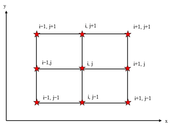
Figure 1.
Distribution of the calculation points.
Then, the residual GA, denoted as , can be derived as Equation (3) [6].
In which,
are the wave number in and direction; denote the wavelength in and direction; ; ; and are reference values of DV, which provide a reference model; F and F−1 are Fast Fourier transform (FFT) and inverse FFT computing.
2.2. Errors in Environmental Correction Simulation
During the simulation of errors in environmental correction, it is assumed that the signal changes in all directions are the same; that is, they are isotropic. Therefore, the wave number spectrum along the orbit can represent the change in its signal in all directions [23]. The two-dimensional spectrum is integrated into the cross-orbit frequency dimension to obtain the one-dimensional spectrum. The two-dimensional spectrum can be expressed as a function of the one-dimensional spectrum [23]:
where is the one-dimensional wave number (or spatial frequency), ; and represent the one-dimensional spectrum and two-dimensional spectrum, respectively.
Assume that the two-dimensional errors in environmental correction are the superposition of multiple two-dimensional random Fourier sequences, the two-dimensional isotropic error value can be obtained from the formula [23,24]:
where is the wave number corresponding to the nth component in direction of and ; is a random phase within the range ; is the error caused by the errors in environmental corrections, constructed as the sum of N random 2D Fourier components from the annulus in the 2D wave-number domain bounded by and [23]. Since the phase of each Fourier component is random, each simulation is random. is set to 2000 in this study.
In this study, the one-dimensional power spectrum of each residual environmental error provided by the SWOT error budget document [25] is used, as shown in Equations (7)–(10). Among them, the wet tropospheric residual error spectrum is derived from the corrected data using the two-beam radiometer [25]; the dry tropospheric residual error spectrum is derived from the Chelton model [19,25]; the ionospheric residual error spectrum is derived using the Ionex model [18]; the wave number spectrum of the SSB residual error is obtained using the four-parameter BM4 parameter model [17].
where represent the one-dimensional power spectrum of errors in the wet troposphere, dry troposphere, ionosphere and sea state bias correction, respectively. To show the magnitude of the errors showed by Equations (7)–(10), Figure 2 presents the values of them in terms of wavelength.
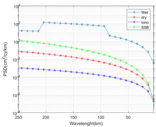
Figure 2.
PSD of errors in environmental corrections.
Based on Equations (7)–(10), we can derive the two-dimensional power spectrum using Equation (5). The SSH errors generated by errors in environmental correction are then obtained using Equation (6).
In the statistics, in addition to indices of mean, standard deviation (STD), max, min, and RMS, the statistical indices mean absolute error (MAE) and relative error (RE) are also used as follows,
In which is the number of the data; means the data; is the true value of the data.
2.3. Data Processing Flow
In the first step, we simulate the true values of gravity field elements using EGM2008 [26], including geoid heights N, DV, and GA, as shown in Equations (13)–(15) [26]:
In the above equations, is Earth gravitational constant; is mean radius of the Earth, while is the semi-major axis of the Earth; , represent degree and order of the gravity field model, respectively; is the largest degree of EGM2008; and denote the difference values of spherical harmonic coefficients of EGM2008 and normal gravity potential; is the fully normalized Legendre function value at degree and order ; is the spherical coordinate of the computing point.
Then, errors in environmental correction are also simulated using Equations (7)–(10). Regardless of the effect of mean dynamic topography, this study assumes that N is equal to SSH. Then, errors in environmental correction are added to N to obtain the simulated SSHs. Finally, we derive DV using the SSHs with or without errors in environmental correction, and GA is also derived correspondingly. By comparing the true values of SSHs, DV, and GA, the impact of errors in environmental correction on gravity field recovery is analyzed. The whole processing flow is shown in Figure 3.
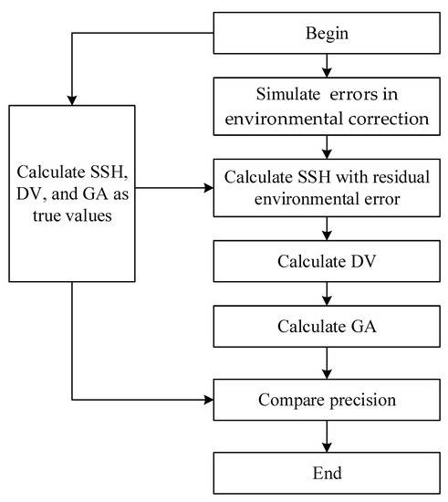
Figure 3.
Data processing flow chart.
3. Data and Study Area
In this study, EGM2008 [26] is used to provide gravity products as the true values, including geoid height used as SSH observations directly, DV, and GA. In the gravity field recovery using SSH, the remove-restore technique is usually used [7,22], and EGM96 is used as the reference model in this study. The study area is located in the South China Sea with longitudes of 111°~112° E, latitudes of 10°30′~12°30′ N. The resolution of the simulated data is 2 km × 2 km. Figure 4 shows the simulated SSH, DV, and GA.
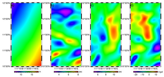
Figure 4.
Simulated data (seen as true values): (a) SSH; (b) North-south component of DV; (c) East-west component of DV; (d) GA.
4. Results and Analysis
4.1. Gravity Field Recovery without Errors in Environmental Correction
To verify the effectiveness of the inversion method used in this study, we first conducted the numerical tests without adding any errors in environmental correction to SSH. The comparisons between the recovered gravity field products and the true values are presented in Figure 5, Figure 6 and Figure 7, and the related statistics are given in Table 1. According to these figures, there are minor computing errors in deriving the two components of DV. According to Table 1, the average absolute error of the north-south component of DV is only 0.007 arcsec, and the average absolute error of the east-west component is about 0.01 arcsec. From the error diagram, the maximum error of the recovered gravity anomaly is about 0.5 mGal, and the average percentage error is 3.48%, which is poorer than that of DV. The main reason is in the derivation of GA, the reference model is used, i.e., EGM96. If a higher accurate model is used, the relative error would be reduced correspondingly. Even so, the above results can verify the effectiveness of the computing method in this study.
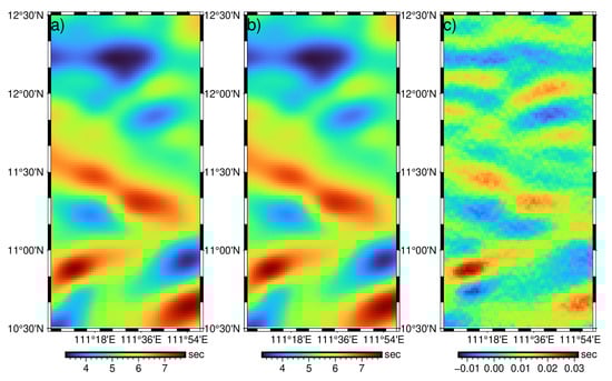
Figure 5.
North-south component of DV: (a) true value; (b) recovered value; (c) error.
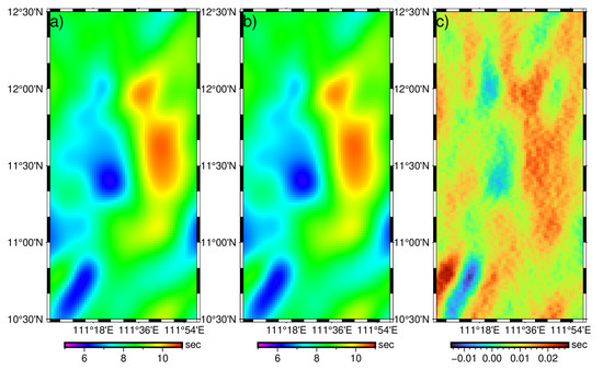
Figure 6.
East-west component of DV: (a) true value; (b) recovered value; (c) error.
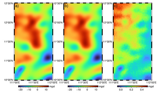
Figure 7.
GA: (a) true value; (b) recovered value; (c) error.

Table 1.
Statistics on the accuracy of the recovered DV and GA.
4.2. Impact of Errors in Environmental Correction on SSH
In actual marine gravity field inversion, more attention is paid to relative height [13]. To analyze the relative height error, the definition of the relative height given by Wan et al. (2020b) [13] is used in this study, i.e., Equation (16). Please note the point distribution has been shown in Figure 1. The reason for defining this relative height is to improve the precision of this value, since this value is derived from mean values of four initial relative heights, i.e., the relative height between the central point and each of the adjacent points (see Equation (16) and Figure 1).
Relative height error is the absolute value of the difference between the value of the relative elevation by adding errors in environmental corrections and the true value is defined as the relative height errors. Absolute height error is defined as follows:
where is the SSH by adding errors in environmental corrections and the true value where is the assumed true SSH.
Figure 8 and Figure 9 present the influence of different errors in environmental correction on absolute height and relative height, and the related statistics are given in Table 2. According to Figure 8, the error of absolute height generated by the wet troposphere is around −1.28~0.87 cm, and the absolute error range of SSH caused by the residual error of SSB is −0.05~0.64 cm. The magnitude of the absolute height error of SSH caused by the dry troposphere and ionosphere is 0.01 cm. Therefore, the wet troposphere and the SSB are the main factors affecting the accuracy of the SSH. Regarding relative height error, the impact of the wet troposphere is 0.023 cm in terms of STD. In contrast, the impact of other errors in environmental correction is smaller than 0.001 cm in terms of STD. This means the error of the wet troposphere is the main factor affecting the relative height accuracy.
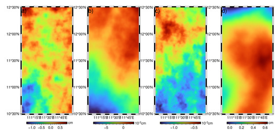
Figure 8.
Absolute height error of SSH caused by: (a) wet troposphere; (b) dry troposphere; (c) ionosphere; (d) SSB.
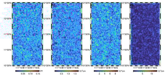
Figure 9.
Relative height errors caused by: (a) wet troposphere; (b) dry troposphere; (c) ionosphere; (d) SSB.
Table 2.
Statistics of the errors caused by residual environmental errors (unit:cm).
4.3. Impact of Errors in Environmental Correction on the Recovery of DV
Figure 10 and Figure 11 present the errors of DV generated by errors in environmental correction and Table 3 summarizes the related statistics. According to Table 3, the maximum absolute error value in the north-south component is about 0.26 arcsec, where it is 0.23 arcsec in the east-west component. The MAE of the two components is smaller than 0.06 arcsec, and the error RMS is smaller than 0.07 arcsec. The relative error is within 1%, which indicates the minor impact on the accuracy of DV.
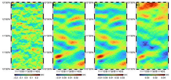
Figure 10.
Error of north-south component of DV caused by: (a) wet troposphere; (b) dry troposphere; (c) ionosphere; (d) SSB.
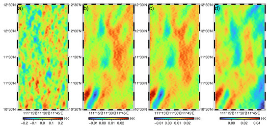
Figure 11.
Error of east-west component of DV caused by: (a) wet troposphere; (b) dry troposphere; (c) ionosphere; (d) SSB.
Table 3.
The Influence of residual environmental errors on the recovery accuracy of DV (uint: arcsec).
Compared to the wet troposphere, the other three types of errors in environmental correction have more negligible impact on the derivation of DV. For example, there is no apparent accuracy loss under these three cases of errors in environmental correction. RMS and MAE of errors do not exceed 0.015 arcsec; RMS and MAE of does not exceed 0.016 arcsec. However, the index for the wet troposphere is at least two times larger than those of the other three types.
The above results indicate that errors in environmental correction will not generate great errors in the derivations of DV. The possible reason is that DV is derived from the differences in computing the geoid heights, and thus the accuracy of DV is mainly determined by relative height accuracy. According to Table 2 (see the results on relative heights), the error magnitude of the relative height of SSH caused by residual errors of the dry troposphere, ionosphere, and SSB is cm. In contrast, the relative height error of SSH caused by the residual environmental errors of the wet troposphere is 0.1 mm. The poorer accuracy of the relative SSH will certainly lead to poorer accuracy of the derived DV. In sum, among the four kinds of residual environmental errors, the wet troposphere has the most significant impact on the calculation of DV, followed by the SSB, and the residual errors in the dry troposphere and ionosphere have the most minor influence on the derivation of DV.
4.4. Influence of Residual Environmental Errors on GA Accuracy
Figure 12 shows the effects of the wet troposphere, dry troposphere, ionosphere, and SSB residual errors on GA recovery. Table 4 gives the statistics on the errors of GA caused by residual environmental errors. Definitely, among the four kinds of residual environmental errors, the wet troposphere residual errors have the most significant impact on the accuracy of GA recovery. For example, it can be seen from Figure 12 that the GA error caused by wet troposphere residual errors reached 2 mGal. From the variation range of error (see Table 4), the variation range of GA error caused by residual wet troposphere errors is about −1.29 mGal~1.99 mGal, and the relative percentage error is 6.42%. In contrast, the other residual environmental errors and calculation errors affect the accuracy of the gravity anomaly in the range of −0.34 mGal~0.50 mGal, and the relative error is about 3.5%.
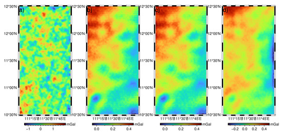
Figure 12.
GA errors caused by: (a) wet troposphere; (b) dry troposphere; (c) ionosphere; (d) SSB.
Table 4.
Statistics of GA errors caused by different residual environmental errors (unit: mGal).
4.5. Comparison in the Spectral Domain
To present the characteristics in the spectral domain, the power spectral density (PSD) of the errors of SSH, DV and GA generated by residual environmental errors are derived, as shown in Figure 13, Figure 14 and Figure 15. In these figures, wet, dry, iono and ssb denote impacts from the wet troposphere, dry troposphere, ionosphere, and residual SSB errors, respectively. According to Figure 13, the wet troposphere has the most significant impact on the SSH accuracy, and is followed by residual SSB errors. It is easy to find that the wet troposphere has the most significant influence on the inversion accuracy of DV and GA, in all the wavelengths shown in Figure 13 and Figure 14. We can also find that SSB has a little more significant influence than dry troposphere and ionosphere, where dry troposphere and ionosphere have almost identical impact on DV and GA inversion accuracy.
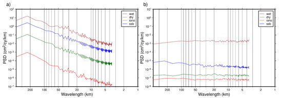
Figure 13.
Error PSD of SSH. (a) absolute height; (b) relative height.
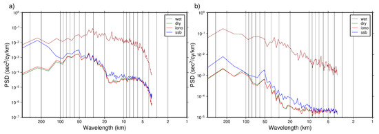
Figure 14.
Error PSD of DV. (a) North-south component; (b) East-west component.
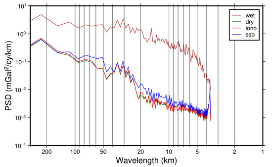
Figure 15.
Error PSD of GA.
5. Discussion
Error in environmental corrections is only one of the factors influencing the gravity field recovery accuracy. To evaluate the influence from other factors, this section carried out a simulation using swot_simulator by considering some of the other errors, including KaRIn error, phase error, roll error, baseline dilation error and timing error (Ubelmann et al., 2014). Since the impact of wet troposphere has the greatest impact on the accuracy of the recovered gravity field products among the aforementioned environmental corrections, this type of error is also considered in the simulation.
We used sea level anomaly (SLA) as the input data to generate SLA observation data on the strip along the ground track. Please note that in this process, the above-mentioned errors are added. In the noise simulation, the significant wave height (SWH) is set as 2 m. The SWOT track uses the scientific track file (ephemeris_science_sept2015_ell.txt) with a revisit cycle of 21 days, downloaded from AVISO (https://www.aviso.altimetry.fr/en/missions/future-missions/swot/orbit.html (accessed on 15 October 2022)). The orbital inclination is 77.68°, and the orbital height is 891 km; the total cutting width is set as 120 km (half_swath = 60.0); the interference baseline length of Ka band (35.75 GHz) is 10 m. These parameters are the same as those of SWOT. The simulation was conducted in the region with longitudes of 110°–113° E and latitudes of 10°–13° N for 1 year at a resolution of 2 km.
The differences between the input SLA data and the output SLA data are seen as the influences from the added errors. Statistics in the region which is introduced in Section 3 (i.e., the region with longitudes of 111°–112° E, and latitudes of 10.5°–12.5° N) are obtained in different time lengths. The variations in the mean, standard deviation (STD) values of the differences are presented in Figure 16.
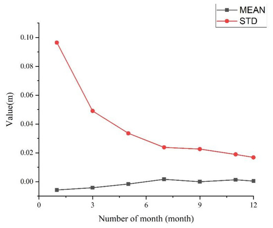
Figure 16.
Variation of the statistics with time length.
It can be seen from Figure 16 that with the growth of the time span and the accumulation of observation data, the statistical values of the residual errors gradually decrease. The error change amplitude in the first five months is large. For example, when the observation data accumulated to 1 month, the error is close to 0.1 m due to the small number of observations. As the data accumulated to 3 months, the STD decreased to about 0.05 m; When the data accumulated to 5 months, the STD decreased to about 0.03 m. It can be seen from the STD curve that as the observation data accumulate from 1 month to more than 5 months, the STD value decreases rapidly, indicating that as the observation time increases (i.e., the amount of data increases) and the random errors can be reduced largely. When the observation data accumulated from 5 months to 12 months, while the STD value still decreased, the rate decreased gradually, and finally converged to around 0.02 m. It indicates that the increase in the amount of observation data can reduce the random error, but it cannot completely overcome the random error, and residual errors still exist.
It needs to be noted that the mean dynamic topography (MDT) and the time-varying ocean signals would influence the gravity recovery accuracy significantly. Although the issue of dynamic topography has been processed well in conventional altimetry processing, such as the usage of the existing MDT model [22,27,28,29], whether the spatial resolution and accuracy are enough should be analyzed further. As for the time-varying ocean signals, such as eddies, front, and even wind waves, long time observations can be used to reduce their effects, such as the errors reduced shown in Figure 16.
6. Conclusions
In this study, four kinds of residual environmental errors, including the wet troposphere, dry troposphere, ionosphere and SSB, are simulated, and then DV and GA are derived using the SSH data by adding the simulated residual environmental errors. The results show that the residual errors of the wet troposphere and SSB have a more significant impact on the absolute error of sea level height; the impact of the wet troposphere residual error on the relative height accuracy is a millimeter, and the corresponding influence of other residual environmental errors is very small. The residual errors of dry troposphere, ionosphere and SSB have little impact on the DV and GA recovery accuracy. In general, among the four kinds of residual environmental errors, the wet troposphere is the main factor affecting the accuracy of DV calculation and GA recovery. The RMS of GA error caused by the wet troposphere is about 0.47 mGal in this study.
It needs to be noted that the wave-number spectrum simulation method in this study depends on some assumptions, such as no correlation between error components. However, it may be not true in actual cases. For example, it is estimated that the residual error of SSB may have a correlation with SSH [30]. Therefore, the correlations between these errors should be investigated in future research. Even so, the results of this study can give an initial evaluation of the residual environmental error on gravity field recovery, at least the magnitudes of the errors caused by them.
On the other hand, since the main advantage of the InRA is the ultra-high spatial resolution, we can mainly use InRA observations to improve the short-wavelength of marine gravity field products. However, according to Figure 15, the error in the long-wavelength part such as the wavelength greater than 50 or 100 km has a larger magnitude compared to the short-wavelength part. Indeed, the long-wavelength of marine gravity field can be provided by a highly accurate background model, i.e., using the remove-restore method [22,28,29]. Additionally, it can be recovered by observations of gravity satellites, such as Gravity field and steady-state Ocean circulation mission (GOCE) [31,32], Gravity Recovery and Climate Experiment (GRACE) [33] and GRACE Follow On. Hence, we can adopt a high-pass filter to remove the long-wavelength errors caused by the environment, although the long-wavelength signals are also removed. This should also be investigated in future research.
Besides the residual environmental errors discussed in this study, there are many other factors affecting the derivation of gravity field products using InRA altimeter observations, such as instrument errors of InRA altimeter [34], which can be caused by phase error, baseline error, rolling angle error, etc. Compared to InRA instrument errors, environmental error is not the limiting factor for highly accurate gravity field recovery. Instead, InRA altimeter system error would be the limitation [13,16], which puts forward high requirements to the related space technology. In addition, how to remove or reduce the observation errors [24] and propose a highly accurate new algorithm for gravity field products are valuable points of study in this field.
Author Contributions
Conceptualization, X.W.; methodology, F.W. and X.W.; software, F.W. and X.W.; investigation, all the authors.; resources, X.W. and B.L.; data curation, F.W. and H.G.; writing—original draft preparation, X.W. and F.W.; writing—review and editing, all the authors.; funding acquisition, X.W. All authors have read and agreed to the published version of the manuscript.
Funding
This study was supported by National Natural Science Foundation of China (No. 42074017) and the Fundamental Research Funds for the Central Universities (No. 2-9-2022-701).
Institutional Review Board Statement
Not applicable.
Informed Consent Statement
Informed consent was obtained from all subjects involved in the study.
Data Availability Statement
The EGM2008 and EGM96 can be downloaded from website: http://icgem.gfz-potsdam.de/home (accessed on 15 October 2022).
Acknowledgments
The authors would like to thank Taoyong Jin for the help of data simulation. We also would like to thank the OceanDataLab for providing the SWOT simulator in the website of https://github.com/SWOTsimulator/swotsimulator (accessed on 15 October 2022).
Conflicts of Interest
The authors declare no conflict of interest.
References
- Zhang, S.; Sandwell, D.T.; Jin, T.; Li, D. Inversion of marine gravity anomalies over southeastern China seas from multi-satellite altimeter vertical deflections. J. Appl. Geophys. 2017, 137, 128–137. [Google Scholar] [CrossRef]
- Watts, A.B.; Tozer, B.; Harper, H.; Boston, B.; Shillington, D.J.; Dunn, R. Evaluation of Shipboard and Satellite-Derived Bathymetry and Gravity Data over Seamounts in the Northwest Pacific Ocean. J. Geophys. Res. Solid Earth 2020, 125, e2020JB020396. [Google Scholar] [CrossRef]
- Li, Z.; Guo, J.; Ji, B.; Wan, X.; Zhang, S. A Review of Marine Gravity Field Recovery from Satellite Altimetry. Remote Sens. 2022, 14, 4790. [Google Scholar] [CrossRef]
- Andersen, O.B.; Knudsen, P.; Berry, P.A.M. The DNSC08GRA global marine gravity field from double retracked satellite altimetry. J. Geod. 2010, 84, 191–199. [Google Scholar] [CrossRef]
- Sandwell, D.T.; Harper, H.; Tozer, B.; Smith, W.H.F. Gravity field recovery from geodetic altimeter missions. Adv. Space Res. 2019, 68, 1059–1072. [Google Scholar] [CrossRef]
- Sandwell, D.T.; Smith, W.H.F. Marine gravity anomaly from Geosat and ERS 1 satellite altimetry. J. Geophys. Res. Solid Earth 1997, 102, 10039–10054. [Google Scholar] [CrossRef]
- Wan, X.; Annan, R.F.; Wang, W. Assessment of HY-2A GM data by deriving the gravity field and bathymetry over the Gulf of Guinea. Earth Planets Space 2020, 72, 151. [Google Scholar] [CrossRef]
- Hwang, C. Inverse Vening Meinesz formula and deflection-geoid formula: Applications to the predictions of gravity and geoid over the South China Sea. J. Geod. 1998, 72, 304–312. [Google Scholar] [CrossRef]
- Esteban-Fernandez, D.; Rodriguez, E.; Fu, L.-L.; Alsdorf, D.; Vaze, P. The Surface Water and Ocean Topography Mission: Centimetric Spaceborne Radar Interferometry. In Sensors, Systems, and Next-Generation Satellites XIV; International Society for Optics and Photonics: Bellingham, WA, USA, 2010; p. 782615. [Google Scholar]
- Fu, L.-L.; Alsdorf, D.; Morrow, R.; Rodriguez, E.; Mognard, N. SWOT: The Surface Water and Ocean Topography Mission: Wide-Swath Altimetric Elevation on Earth; Jet Propulsion Laboratory, National Aeronautics and Space Administration: Pasadena, CA, USA, 2012. [Google Scholar]
- Yan, J. System Design and Performance Analysis of 3D-Imaging Altimeter. Ph.D. Thesis, Center for Space Science and Applied Research, Chinese Academy of Science, Beijing, China, 2005. [Google Scholar]
- Ren, L.; Yang, J.; Dong, X.; Zhang, Y.; Jia, Y. Preliminary Evaluation and Correction of Sea Surface Height from Chinese Tiangong-2 Interferometric Imaging Radar Altimeter. Remote Sens. 2020, 12, 2496. [Google Scholar] [CrossRef]
- Wan, X.; Jin, S.; Liu, B.; Tian, S.; Kong, W.; Annan, R.F. Effects of Interferometric Radar Altimeter Errors on Marine Gravity Field Inversion. Sensors 2020, 20, 2465. [Google Scholar] [CrossRef]
- Miao, X.; Wang, J.; Mao, P.; Miao, H. Cross-Track Error Correction and Evaluation of the Tiangong-2 Interferometric Imaging Radar Altimeter. IEEE Geosci. Remote Sens. Lett. 2022, 19, 1–5. [Google Scholar] [CrossRef]
- Yu, D.; Hwang, C.; Andersen, O.B.; Chang, E.T.Y.; Gaultier, L. Gravity recovery from SWOT altimetry using geoid height and geoid gradient. Remote Sens. Environ. 2021, 265, 112650. [Google Scholar] [CrossRef]
- Jin, T.; Zhou, M.; Zhang, H.; Li, J.; Jiang, W.; Zhang, S.; Hu, M. Analysis of vertical deflections determined from one cycle of simulated SWOT wide-swath altimeter data. J. Geod. 2022, 96, 30. [Google Scholar] [CrossRef]
- Gaspar, P.; Ogor, F.; Le Traon, P.-Y.; Zanife, O.-Z. Estimating the sea state bias of the TOPEX and POSEIDON altimeters from crossover differences. J. Geophys. Res. Oceans 1994, 99, 24981–24994. [Google Scholar] [CrossRef]
- Schaer, S.; Gurtner, W.; Feltens, J. IONEX: The Ionosphere Map Exchange Format Version 1. In Proceedings of the 1998 IGS Analysis Centers Workshop, ESOC, Darmstadt, Germany, 9–11 February 1998. [Google Scholar]
- Fu, L.-L.; Cazenave, A. Satellite Altimetry and Earth Sciences: A Handbook of Techniques and Applications, 2nd ed.; Academic Press: New York, NY, USA, 2000; pp. 1–122. [Google Scholar]
- Brown, S. A Novel Near-Land Radiometer Wet Path-Delay Retrieval Algorithm: Application to the Jason-2/OSTM Advanced Microwave Radiometer. IEEE Trans. Geosci. Remote Sens. 2010, 48, 1986–1992. [Google Scholar] [CrossRef]
- Wan, X.; Annan, R.F.; Jin, S.; Gong, X. Vertical Deflections and Gravity Disturbances Derived from HY-2A Data. Remote Sens. 2020, 12, 2287. [Google Scholar] [CrossRef]
- Wan, X.; Hao, R.; Jia, Y.; Wu, X.; Wang, Y.; Feng, L. Global marine gravity anomalies from multi-satellite altimeter data. Earth Planets Space 2022, 74, 165. [Google Scholar] [CrossRef]
- Ubelmann, C.; Fu, L.-L.; Brown, S.; Peral, E.; Esteban-Fernandez, D. The Effect of Atmospheric Water Vapor Content on the Performance of Future Wide-Swath Ocean Altimetry Measurement. J. Atmos. Ocean. Technol. 2014, 31, 1446–1454. [Google Scholar] [CrossRef]
- Zhou, M.; Jin, T.; Jiang, W. The Wet Tropospheric Correction of Wide-Swath Altimeter Using Optimum Interpolation Method. Geomat. Inf. Sci. Wuhan Univ. 2021. [Google Scholar] [CrossRef]
- Esteban-Fernandez, D.; Pollard, B.; Vaze, P.; Abelson, R. SWOT Project Mission Performance and Error Budget; Jet Propulsion Laboratory Document D-79084 Revision A; National Aeronautics and Space Administration: Pasadena, CA, USA, 2017. [Google Scholar]
- Pavlis, N.K.; Holmes, S.A.; Kenyon, S.C.; Factor, J.K. The development and evaluation of the Earth Gravitational Model 2008 (EGM2008). J. Geophys. Res. Solid Earth 2012, 117, B04406. [Google Scholar] [CrossRef]
- Barthelmes, F. Defnition of Functionals of the Geopotential and Their Calculation from Spherical Harmonic Models: Theory and Formulas Used by the Calculation Service of the International Centre for Global Earth Models (ICGEM); Deutsches Geo Forschungs Zentrum GFZ: Potsdam, Germany, 2013. [Google Scholar] [CrossRef]
- Zhang, S.; Zhou, R.; Jia, Y.; Jin, T.; Kong, X. Performance of HaiYang-2 altimetric data in marine gravity research and a new global marine gravity model NSOAS22. Remote Sens. 2022, 14, 4322. [Google Scholar] [CrossRef]
- Zhu, C.; Guo, J.; Yuan, J.; Li, Z.; Liu, X.; Gao, J. SDUST2021GRA: Global marine gravity anomaly model recovered from Ka-band and Ku-band satellite altimeter data. Earth Syst. Sci. Data 2022, 14, 4589–4606. [Google Scholar] [CrossRef]
- Ubelmann, C.; Dibarboure, G.; Dubois, P. A Cross-Spectral Approach to Measure the Error Budget of the SWOT Altimetry Mission over the Ocean. J. Atmos. Ocean. Technol. 2018, 35, 845–857. [Google Scholar] [CrossRef]
- Pail, R.; Goiginger, H.; Schuh, W.D.; Höck, E.; Brockmann, J.M.; Fecher, T.; Gruber, T.; Mayer-Gürr, T.; Kusche, J.; Jäggi, A.; et al. Combined satellite gravity field model GOCO01S derived from GOCE and GRACE. Geophys. Res. Lett. 2010, 37, L20314. [Google Scholar] [CrossRef]
- Wan, X.; Yu, J. Derivation of the radial gradient of the gravity based on non-full tensor satellite gravity gradients. J. Geodyn. 2013, 66, 59–64. [Google Scholar] [CrossRef]
- Tapley, B.D.; Bettadpur, S.; Watkins, M.; Reigber, C. The gravity recovery and climate experiment: Mission overview and early results. Geophys. Res. Lett. 2004, 31, L019779. [Google Scholar] [CrossRef]
- Gaultier, L.; Ubelmann, C.; Fu, L.-L. The Challenge of Using Future SWOT Data for Oceanic Field Reconstruction. J. Atmos. Ocean. Technol. 2016, 33, 119–126. [Google Scholar] [CrossRef]
Publisher’s Note: MDPI stays neutral with regard to jurisdictional claims in published maps and institutional affiliations. |
© 2022 by the authors. Licensee MDPI, Basel, Switzerland. This article is an open access article distributed under the terms and conditions of the Creative Commons Attribution (CC BY) license (https://creativecommons.org/licenses/by/4.0/).