Appendix B
The loss curves and validation metrics for each trained model are presented in
Figure A3,
Figure A4,
Figure A5,
Figure A6,
Figure A7,
Figure A8,
Figure A9,
Figure A10,
Figure A11,
Figure A12,
Figure A13,
Figure A14 and
Figure A15. The models are explained in
Table 4.
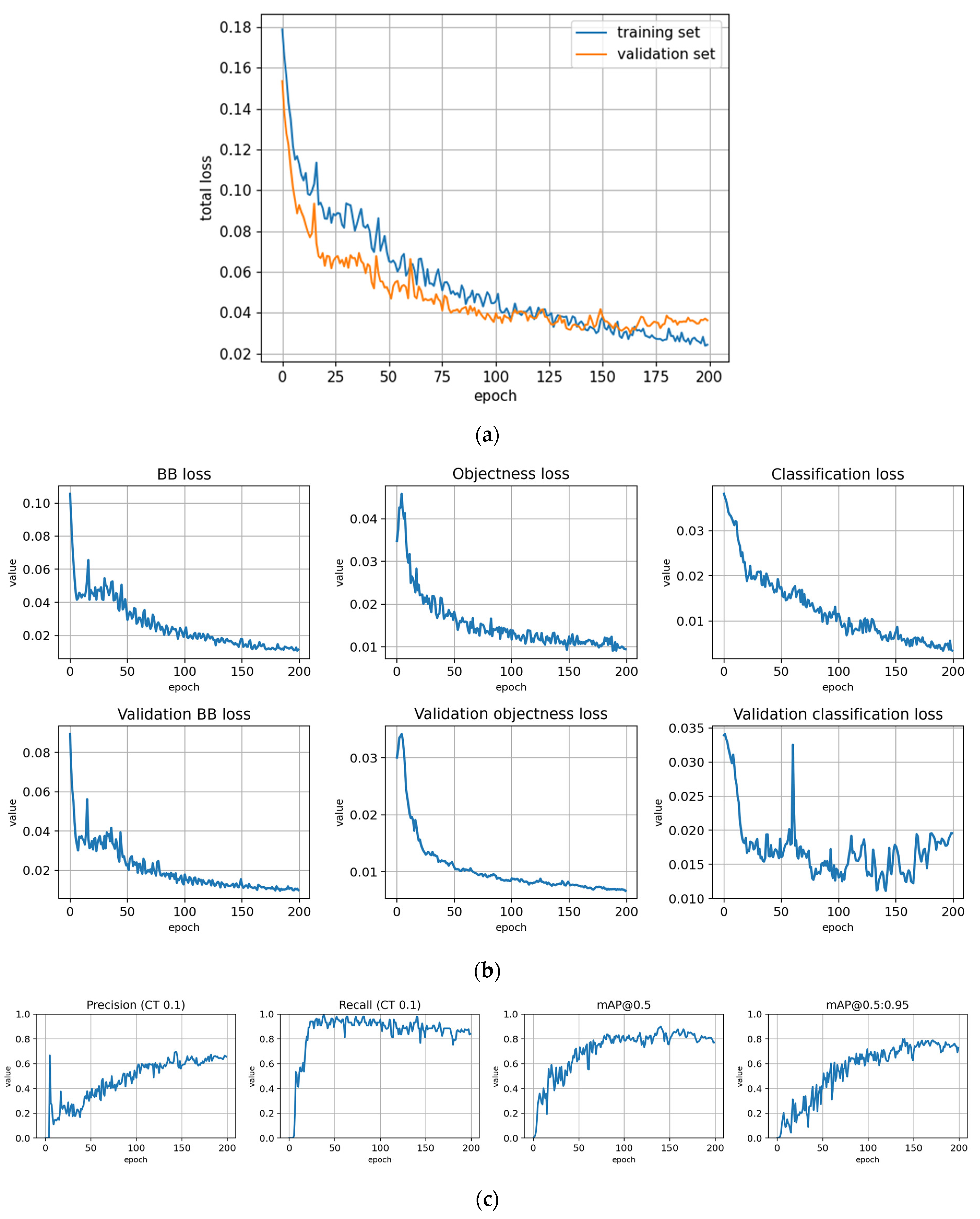
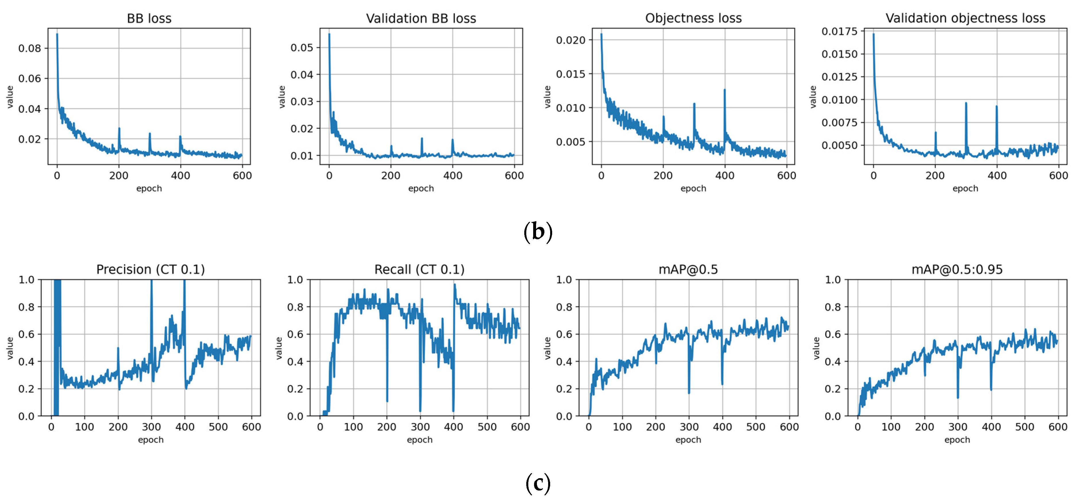
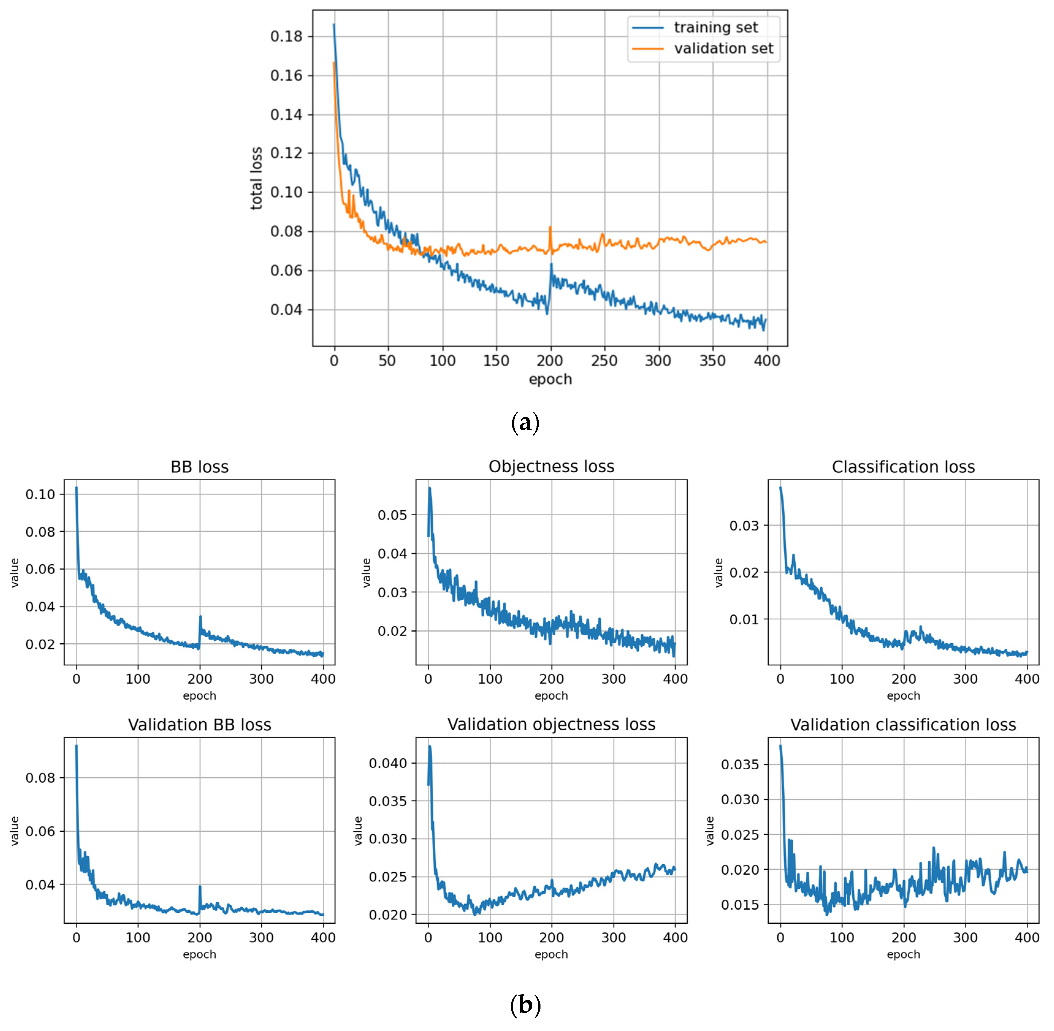
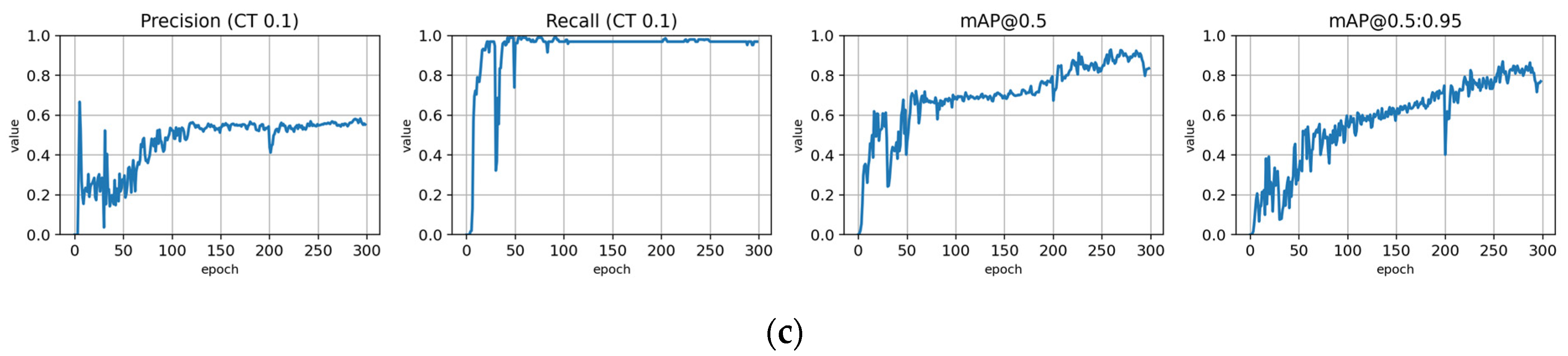
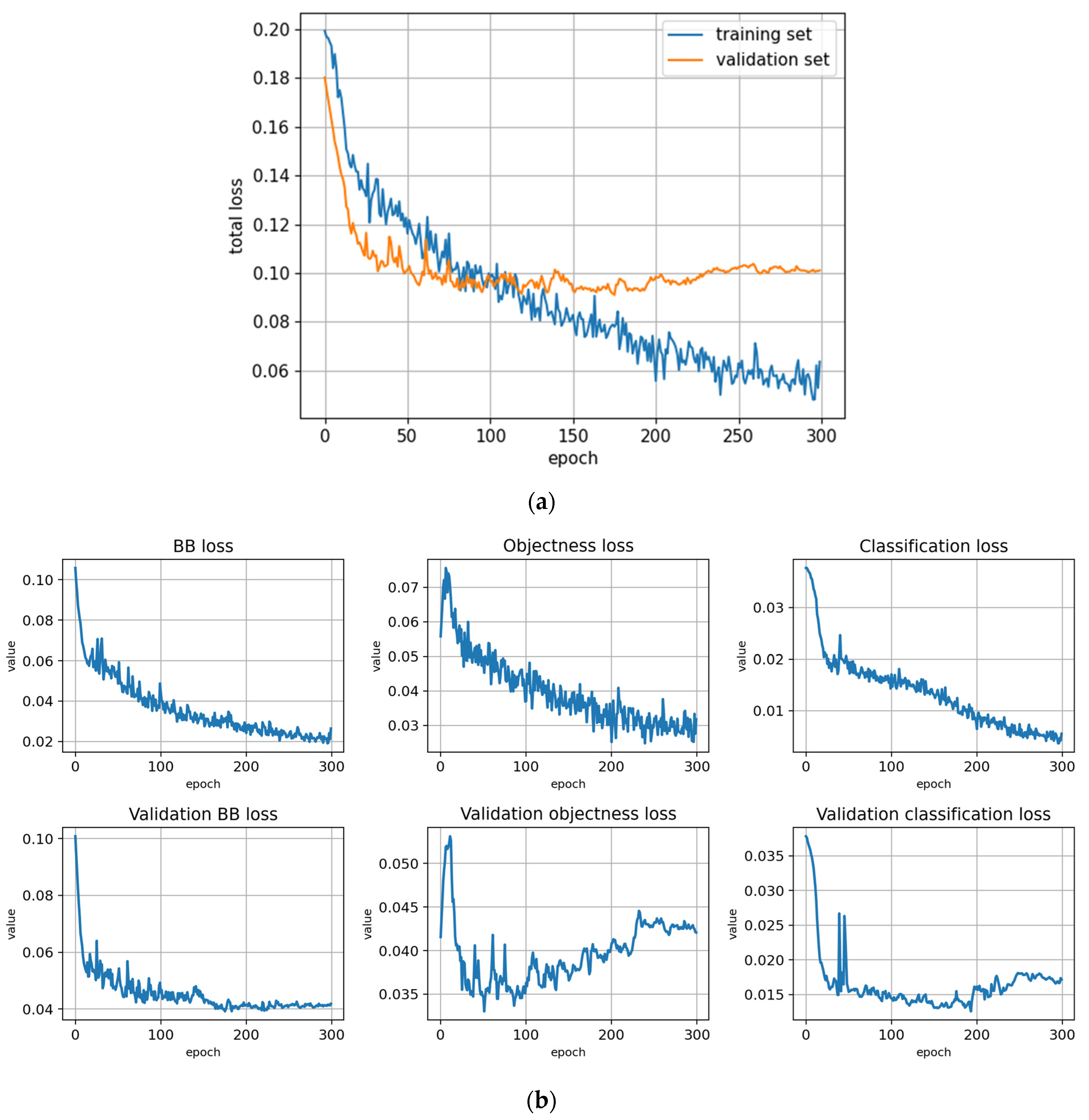
Figure A3.
Training with the Full dataset using classification rule A and optimized hyperparameters (model: trFull-syrA-hyopt). (a) Total loss on the training and validation datasets during training. (b) Loss components during training. Bounding box (BB), objectness, and classification losses are given for the training (top) and validation (bottom) datasets. (c) Precision, Recall, mAP@0.5, and mAP@0.5:0.95 are presented for the validation dataset. CT: confidence threshold.
Figure A4.
Training with the Paloheinä dataset using symptom rule A (model: trPH-syrA). (a) Total loss on the training and validation datasets during training. (b) Loss components during training. Bounding box (BB), objectness, and classification losses are given for the training (top) and validation (bottom) datasets. (c) Precision, Recall, mAP@0.5 and mAP@0.5:0.95 are presented for the validation dataset with CT: confidence threshold.
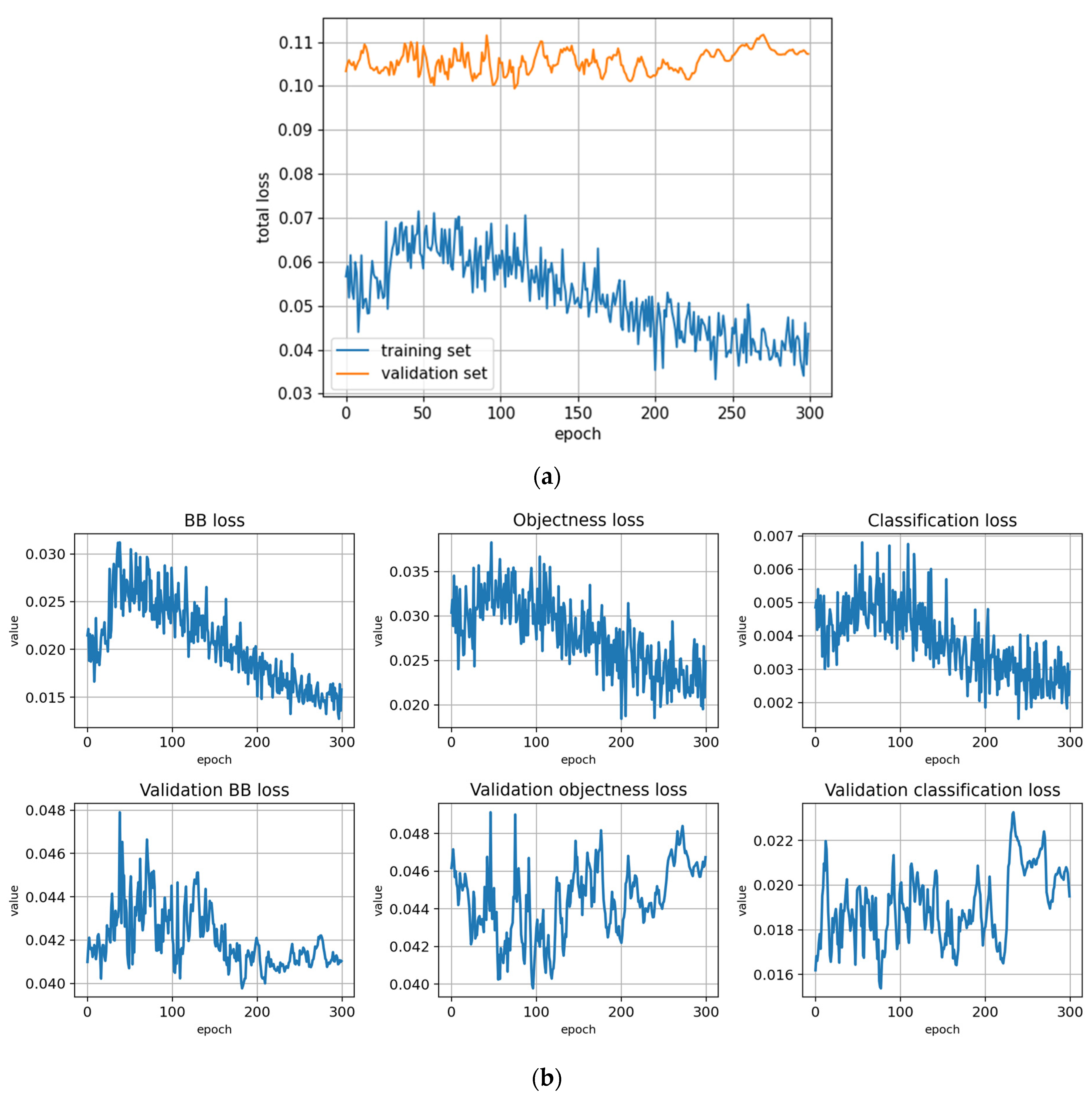
Figure A5.
Fine-tuning the trFull-syrA model with the Paloheinä dataset using symptom rule A (model: trFull-syrA-PHft). (a) Total loss on the training and validation datasets during training. (b) Loss components during training. Bounding box (BB loss), objectness, and classification losses are given for the training (top) and validation (bottom) datasets. (c) Precision, Recall, mAP@0.5 and mAP@0.5:0.95 are presented for the validation dataset. CT: confidence threshold.
Figure A6.
Training with the Lahti-Ruokolahti dataset using symptom rule A (model: trLR-syrA). (a) Total loss on the training and validation datasets during training. (b) Loss components during training. Bounding box (BB loss), objectness, and classification losses are given for the training (top) and validation (bottom) datasets. (c) Precision, Recall, mAP@0.5 and mAP@0.5:0.95 are presented for the validation dataset. CT: confidence threshold.
Figure A7.
Fine-tuning the trFull-syrA model with the Lahti-Ruokolahti dataset using symptom rule A (model: trFull-syrA-LRft). (a) Total loss on the training and validation datasets during training. (b) Loss components during training. Bounding box (BB loss), objectness, and classification losses are given for the training (top) and validation (bottom) datasets. (c) Precision, Recall, mAP@0.5, and mAP@0.5:0.95 are presented for the validation dataset. CT: confidence threshold.
Figure A8.
Training to detect dead trees with the Full dataset using symptom rule A (model: syrA-dead). (a) Total loss on the training and validation datasets during training. (b) Loss of components during training. Bounding box (BB loss), objectness, and classification losses are given for the training and validation datasets. (c) Precision, Recall, mAP@0.5 and mAP@0.5:0.95 are presented for the validation dataset. CT: confidence threshold.
Figure A9.
Training to detect infested trees with the Full dataset using symptom rule A (model: syrA-infested). (a) Total loss on the training and validation datasets during training. (b) Loss components during training. Bounding box (BB loss), objectness, and classification losses are given for the training and validation datasets. (c) Precision, Recall, mAP@0.5, and mAP@0.5:0.95 are presented for the validation dataset. CT: confidence threshold.
Figure A10.
Training with the Full dataset using symptom rule B (model: trFull-syrB). (a) Total loss on the training and validation datasets during training. (b) Loss components during training. Bounding box (BB loss), objectness, and classification losses are given for the training (top) and validation (bottom) datasets. (c) Precision, Recall, mAP@0.5, and mAP@0.5:0.95 are presented for the validation dataset. CT: confidence threshold.
Figure A11.
Training with the Full dataset using symptom rule B and optimized hyperparameters (model: trFull-syrB-hyopt). (a) Total loss on the training and validation datasets during training. (b) Loss components during training. Bounding box (BB loss), objectness, and classification losses are given for the training (top) and validation (bottom) datasets. (c) Precision, Recall, mAP@0.5, and mAP@0.5:0.95 are presented for the validation dataset. CT: confidence threshold.
Figure A12.
Training with the Paloheinä dataset using symptom rule B (model: trPH-syrB). (a) Total loss on the training and validation datasets during training. (b) Loss components during training. Bounding box (BB loss), objectness, and classification losses are given for the training (top) and validation (bottom) datasets. (c) Precision, Recall, mAP@0.5 and mAP@0.5:0.95 are presented for the validation dataset. CT: confidence threshold.
Figure A13.
Fine-tuning the trFull-clrB model with the Paloheinä dataset using symptom rule B (model: trFull-syrB-PHft). (a) Total loss on the training and validation datasets during training. (b) Loss components during training. Bounding box (BB loss), objectness, and classification losses are given for the training (top) and validation (bottom) datasets. (c) Precision, Recall, mAP@0.5, and mAP@0.5:0.95 are presented for the validation dataset. CT: confidence threshold.
Figure A14.
Training with the Lahti-Ruokolahti dataset using symptom rule B (trLR-syrB). (a) Total loss on the training and validation datasets during training. (b) Loss of components during training. Bounding box (BB loss), objectness, and classification losses are given for the training (top) and validation (bottom) datasets. (c) Precision, Recall, mAP@0.5, and mAP@0.5:0.95 are presented for the validation dataset. CT: confidence threshold.
Figure A15.
Fine-tuning the trFull-syrB model with the Lahti-Ruokolahti dataset using symptom rule B (model: trFull-syrB-LRft). (a) Total loss on the training and validation datasets during training. (b) Loss components during training. Bounding box (BB loss), objectness, and classification losses are given for the training (top) and validation (bottom) datasets. (c) Precision, Recall, mAP@0.5, and mAP@0.5:0.95 are presented for the validation dataset. CT: confidence threshold.


 ,
, 


