Article

Modelling the Dynamics of Carbon Storages for Pinus densata Using Landsat Images in Shangri-La Considering Topographic Factors

1
College of Forestry, Southwest Forestry University, Kunming 650224, China
2
Institute of Southwest Survey and Planning, National Forestry and Grassland Administration, Kunming 650021, China
3
Ministry of Education Key Laboratory for Biodiversity Science and Ecological Engineering, Institute of Biodiversity Science, Fudan University, Shanghai 200438, China
4
Research Institute of Forestry Policy and Information, Chinese Academy of Forestry, Beijing 100091, China
*
Author to whom correspondence should be addressed.
Remote Sens. 2022, 14(24), 6244; https://doi.org/10.3390/rs14246244
Submission received: 12 November 2022 / Revised: 4 December 2022 / Accepted: 6 December 2022 / Published: 9 December 2022
(This article belongs to the Special Issue Monitoring Forest Carbon Sequestration with Remote Sensing)

Abstract

:
Accurate estimation of forest carbon storage is essential for understanding the dynamics of forest resources and optimizing decisions for forest resource management. In order to explore the changes in the carbon storage of Pinus densata in Shangri-La and the influence of topography on carbon storage, two dynamic models were developed based on the National Forest Inventory (NFI) and Landsat TM/OLI images with a 5-year interval change and annual average change. The three modelling methods used were partial least squares (PLSR), random forest (RF) and gradient boosting regression tree (GBRT). Various spectral and texture features of the images were calculated and filtered before modelling. The terrain niche index (TNI), which is able to reflect the combined effect of elevation and slope, was added to the dynamic model, the optimal model was selected to estimate the carbon storage, and the topographic conditions in areas of change in carbon storage were analyzed. The results showed that: (1) The dynamic model based on 5-year interval change data performs better than the dynamic model with annual average change data, and the RF model has a higher accuracy compared to the PLSR and GBRT models. (2) The addition of TNI improved the accuracy, in which R2 is improved by up to 10.48% at most, RMSE is reduced by up to 7.32% at most, and MAE is reduced by up to 8.89% at most, and the RF model based on the 5-year interval change data has the highest accuracy after adding TNI, with an R2 of 0.87, an RMSE of 3.82 t-C·ha−1, and a MAE of 1.78 t-C·ha−1. (3) The direct estimation results of the dynamic model showed that the carbon storage of Pinus densata in Shangri-La decreased in 1987–1992 and 1997–2002, and increased in 1992–1997, 2002–2007, 2007–2012, and 2012–2017. (4) The trend of increasing or decreasing carbon storage in each period is not exactly the same on the TNI gradient, according to the dominant distribution, as topographic conditions with lower elevations or gentler slopes are favorable for the accumulation of carbon storage, while the decreasing area of carbon storage is more randomly distributed topographically. This study develops a dynamic estimation model of carbon storage considering topographic factors, which provides a solution for the accurate estimation of forest carbon storage in regions with a complex topography.

1. Introduction

Forests are the mainstay of terrestrial ecosystems, which store 60% of the carbon in the terrestrial ecosystem [1]. Forests play an indispensable role in balancing and regulating CO2 in the atmosphere with their powerful carbon sink function. Global warming is a great threat to humanity today, and the excessive emissions of greenhouse gases, of which CO2 is an important member, is one of the main reasons for global warming. Atmospheric CO2 concentrations have risen dramatically over the past 100 years (they have risen by approximately 110 ppm) [2], a phenomenon that has accelerated the rate of global warming. The accurate estimation of forest carbon storage is related to the ability to reduce atmospheric CO2 concentration. Against this background, the necessity of the study of forest carbon storage is revealed and its accurate estimation is an important basis for regional and even global carbon change studies.
The methods for estimating forest carbon storage includes both traditional direct measurement methods and indirect estimation methods based on remote sensing [3,4]. The traditional method is based on sample site survey and data statistics, which require a large investment of human and financial resources [5], and due to cost and time constraints, there are significant limitations regarding the large range of study objectives and long study periods. In contrast, remote sensing-based methods have the characteristics of being fast, low-cost, large-scale, and less destructive [1,6]. With the rapid development of quantitative remote sensing technology, the results of carbon storage estimation based on remote sensing have become more and more stable and reliable. Therefore, the use of remote sensing methods for the quantitative estimation of forest carbon storage on a larger scale has become a major current trend [7,8].
At present, there is a significant amount of research in remote sensing estimation, and while scholars in various fields have constructed different remote sensing models [9], most of these are static models. The static model is a model developed directly from the attribute values of the sample sites and the remotely sensed feature values of the corresponding points, which are uncalculated state data. If these values are further processed and calculated to produce different types of change values (periodic change, annual average change, rate of change, etc.), then the model developed using these change data is the dynamic model. Change data can describe the different processes of change in forest ecosystems at a given time and have the ability to monitor forest dynamics [10]. Gómez et al. [11] and Zhang et al. [12] compared static models with dynamic models and showed that dynamic models have higher accuracy and better predictive power than static models, with the highest R2 for dynamic models in their study being 0.90 and 0.94, respectively. In the study of forest dynamics, the dynamic model is able to directly estimate the corresponding level of forest change and directly respond to forest dynamics, which improves the efficiency of the long-term forest dynamics study. The calculation of change data needs to be supported by multi-period data. The current National Forest Inventory (NFI) projects in many countries provide the possibility for long-term forest dynamics modelling studies. The ongoing NFI projects in many countries and open-access Landsat time series data offer the potential for long-term forest dynamics modelling studies.
Trees accumulate carbon mainly through photosynthesis during growth, and topographical factors influence the photosynthetic effect by affecting light and water conditions in the environment, which eventually affects the carbon storage of trees [13]. Therefore, topographic factors are an important concern in forest carbon storage studies. The digital elevation model (DEM) provides valuable topographic information including elevation, slope, and aspect [14]. These topographic factors are often used as independent factors in various studies because they do not require complex calculations and processing, are relatively easy to obtain, and reflect the effects of topography on different aspects of vegetation to some extent [15]. However, the influence of topography on forest carbon storage is the result of the combined effect of various topographic factors, and it is difficult to reflect this combined effect by a single elevation or slope. The terrain niche index (TNI) combines elevation and slope information, which is able to reflect the spatial variability of regional elevation and slope [16,17]. Therefore, in past studies, it has been frequently applied to land use change, landscape patterns and ecological effects [18,19]. The topography of forest ecosystems is complex and diverse, so the comprehensive influence of topographic factors should also be considered when modelling carbon storage. The change data can reflect the degree of change in forest carbon storage, and TNI can reflect the comprehensive influence of topographic factors on forest carbon storage, so the combination of the two is important for the accurate estimation of change in forest carbon storage in areas with complex topography.
Shangri-La, Yunnan Province, is rich in forest resources, and Pinus densata is one of the major tree species, which is widely distributed and has an essential impact on the carbon balance of the region. This region is located at the edge of the Tibetan Plateau, with an overall high altitude, and the terrain comprises high mountains and deep valleys with large topographic undulations, making it more difficult to estimate the forest carbon storage in this region accurately. Therefore, in this study, we used the remote sensing dynamic model combined with TNI to estimate the carbon storage of Pinus densata in Shangri-La. The main objectives are the following: (1) developing the carbon storage dynamics model based on two different kinds of change data; (2) exploring the impact of TNI on carbon storage models; and (3) estimating the historical carbon storage changes of Pinus densata in Shangri-La and analyzing the topographic effects of carbon storage changes.

2. Materials and Methods

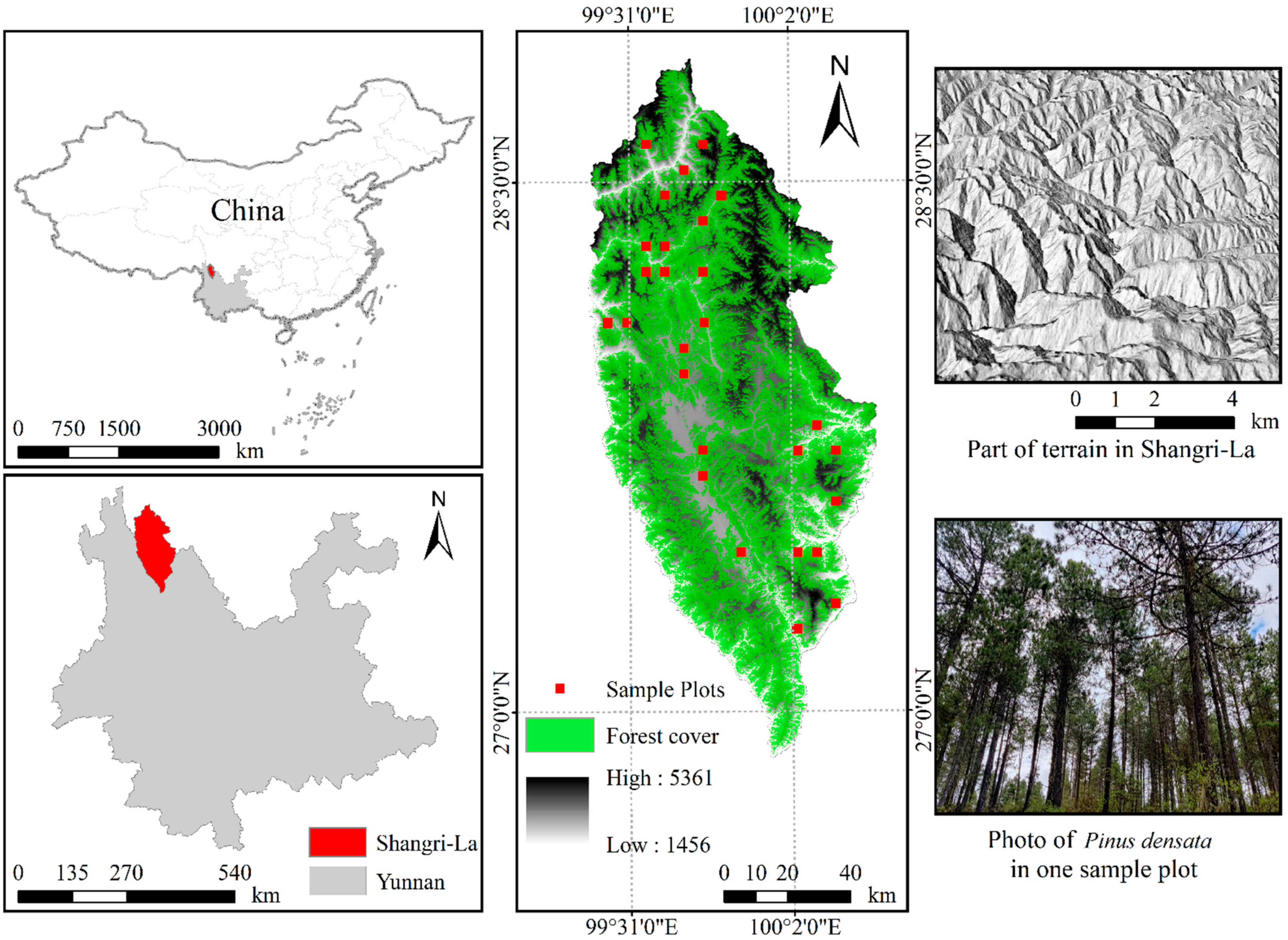
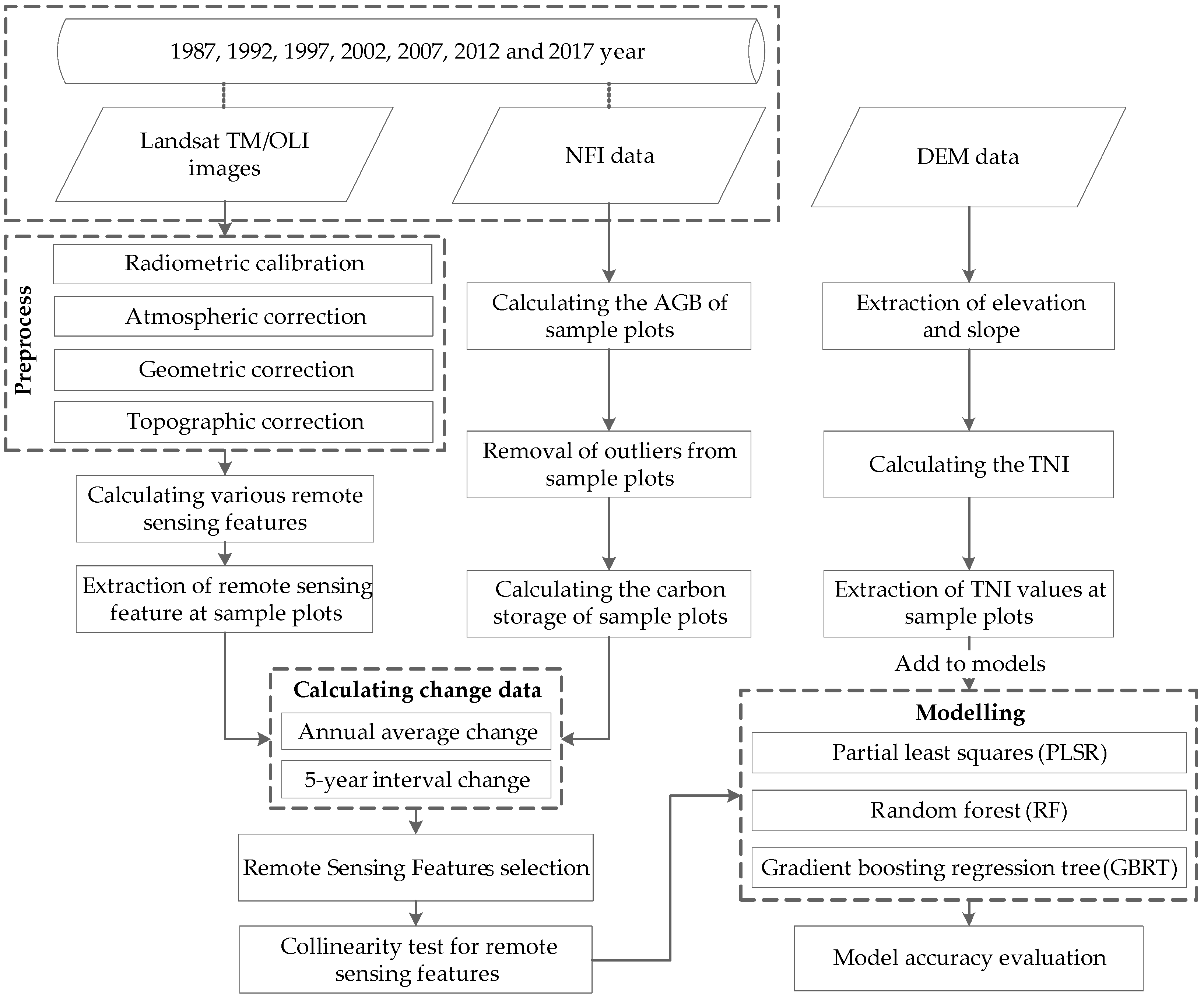
2.1. Study Area and Study Process

The study area, Shangri-La, is located in Yunnan Province in southwestern China (Figure 1), at the border of the Yunnan Province and the Sichuan Province, and the geographical coordinates range from 99°20′ to 100°19′ eastern longitude and 26°52′ to 28°52′ northern latitude, the total area is 1.16 × 10⁶ ha. The area is located in the southeastern part of the Tibetan Plateau (the average elevation is 3459 m), with the Hengduan Mountains running north and south through the whole territory, the regional topography is undulating [20], and the whole terrain is high in the northwest and low in the southeast. Shangri-La has a remarkable monsoon climate, with rainfall concentrated in the months of June to October each year [21], the average annual precipitation is 268~945 mm, and the annual sunshine is 1742.9~2186.6 h. This region is very rich in forest resources, with 76% of forest cover [22]. Pinus densata, Pinus yunnanensis, and Picea asperata are the main tree species in the region [23]. The target species for this study is the Pinus densata, which includes both artificial and natural forests distributed within the study area.
The main content of the study is shown in Figure 2. The research process began with the pre-processing of all the data; then, two types of change data (annual average change and 5-year interval change) were calculated, three methods were used to construct the model, and TNI was added to the model. Finally, in order to compare the effect of the dynamic model with different change data and to compare the effect of the model before and after the addition of TNI, different indicators were used to evaluate the accuracy.

2.2. Ground Survey Data and Carbon Storage Calculation

This study focused on Pinus densata, and the ground survey data were obtained from the National Forestry Inventory, which contains a total of 136 Pinus densata sample plots (comprising pure forests of Pinus densata or forests with Pinus densata as the main species). The years of the collection were 1987, 1992, 1997, 2002, 2007, 2012 and 2017, where the number of sample plots was 19, 22, 23, 16, 16, 17 and 23 for each year, respectively (Figure 3). The dataset records information on tree height, diameter at breast height (DBH), number of trees, coordinate location, and major tree species. The distance between the sample plots consisted of regular distributions of 6 km × 8 km, and each sample plot was a rectangle of 28.28 m × 28.28 m (0.08 ha).
The aboveground biomass (AGB) of the sample plots was calculated based on the allometric growth equation of Pinus densata [24]. The average AGB was first calculated using the average tree height and average DBH of the sample plots. Then, the total AGB of the sample plots was calculated based on the average AGB and the number of Pinus densata. The allometric growth equation is as follows:
            AGB 1 = 0.073 × DBH 1.739 × H 0.880
where AGB1 is single wood aboveground biomass (t), DBH is the diameter at breast height (cm), and H is tree height (m). We filtered the sample plot data. In this process, five sample plots with an AGB (AGB < 1 t·ha−1) that was too small were removed, followed by six outliers that were screened out and removed using the Pauta criterion [25]. According to the Pauta criterion, if a value is outside the range of three times the standard deviation of the mean (outside the range of x ¯ ± 3 σ , where x ¯ is the mean and σ is the standard deviation), it is considered an outlier. This is a common method for outlier screening [26]. In the end, 125 sample plots of Pinus densata remained.
The carbon storage of the sample sites was calculated using the AGB multiplied by the carbon content coefficient. According to the guidelines for measuring carbon storage in forest ecosystems issued by the State Forestry and Grassland Administration of China [27], the average carbon content in the dry matter of Pinus densata is 0.501. The equation is as follows:
              CS = 0.501 × AGB 2
where CS is the carbon storage (t-C·ha−1), and AGB2 is the aboveground biomass of the sample plots (t·ha−1). The basic sample data is shown in Figure 4. The box plots (Figure 4) depict information on the diameter at breast height, tree height, and carbon storage for each year of the sample plots. The overall range of DBH is 6.0–91.7 cm, with a maximum annual mean of 32.0 cm and a maximum annual standard deviation of 27.8 cm; the overall range of tree height is 1.5–24.8 m, with a maximum annual mean of 11.4 m and a maximum annual standard deviation of 5.5 m; and the overall range of carbon storage is 0.7–84.2 t-C·ha−1, with a maximum annual mean of 38.6 t-C·ha−1 and a maximum annual standard deviation of 41.9 t-C·ha−1.

2.3. Remote Sensing Images and Obtained Features

2.3.1. Remote Sensing Data

The remote sensing images used in this study were obtained from the USGS website (http://glovis.usgs.gov/ (accessed on 28 October 2021)). Landsat 5 TM images from 1987, 1992, 1997, 2002, 2007, and 2012 and Landsat 8 OLI images from 2017 of the Shangri-La region were downloaded from the website (Table 1), comprising 21 views in total and a spatial resolution of 30 m. When an image contains too much cloud or is of poor quality, we chose an image from a neighboring timepoint to replace it. Most of the selected images contained less than 5% cloud, and the cloud did not cover the study area when the cloud content was greater than 5%.
In order to improve the image quality, all the images were preprocessed: firstly, radiometric calibration was performed, which converts the original DN (digital number) value of the image to a consistent radiometric brightness in order to eliminate the influence of the sensor [28]; secondly, the Fast Line-of-sight Atmospheric Analysis of Spectral Hypercubes (FLAASH) method was used to eliminate the influence of the atmosphere [29]; thirdly, geometric correction was performed on each image with reference to the existing standard SPOT-5 images to eliminate geometric errors, where the error in geometric correction was less than one pixel; and finally, in order to eliminate the change of image grey value caused by the topographic undulation, topographic correction was performed using the slope matching model [30]. After topographic correction, the brightness of the illuminated side was suppressed and the brightness of the shadow side was enhanced, which better restored the reflectance of the hidden features in the shadow of the original image [31].

2.3.2. Remote Sensing Features

The remote sensing pixel values were evaluated by considering bands with the same name and close wavelengths in Landsat 8 and Landsat 5. In this study, two types of remote sensing features, spectral features and texture features, are calculated. Spectral features are the most basic and direct features of remote sensing images, but the phenomena of “the same objects with different spectra” and “different objects with the same spectra” commonly exist in remote sensing images, so it may be difficult to obtain good research results when only relying on spectral features [32,33]. The texture features can describe the grey scale information of an image, express the spatial distribution of the grey scale of pixels in the image, and reflect the structural information of the image. Compared with spectral features, texture features are less affected by the environment and more stable in information representation [34]. Therefore, the combination of spectral and textural features can effectively reflect the characteristics of the ground objects and their changes [35,36]. A total of 35 spectral features and 540 texture features were obtained in this study (the calculations of various types of textures from all single bands of each image in odd windows from 1 to 19) (Table 2).

2.4. Terrain Niche Index

To explore the influence of elevation and slope on the carbon storage dynamics model, the terrain niche index (TNI), a composite factor combining elevation and slope, was established in this study [41]. Elevation and slope were extracted from the digital elevation model (DEM). The DEM used in this study was an ASTER GDEM data product with a spatial resolution of 30 m. The DEM was downloaded from the Geospatial Data Cloud website (http://www.gscloud.cn/ (accessed on 18 August 2022)). The equation for TNI is as follows:
TNI = log [ ( E E ¯ + 1 ) × ( S S ¯ + 1 ) ]
where E and S are the elevation and slope of any point, respectively, and E ¯ and S ¯ are the average elevation and average slope of the study area, respectively. A larger TNI value indicates a higher elevation and slope; a smaller TNI value indicates a lower elevation and gentler slope; and a medium TNI value indicates a high elevation gentle slope, or a low elevation steep slope, or a medium elevation and slope [42].

2.5. Distribution Index

The distribution index (DI) is often used to show the distribution of various land use types. In this study, the areas of the increasing and decreasing carbon storage of Pinus densata were considered as two different land classes. Then, the DI was used to explore the distribution of carbon storage changes in different TNI gradients. The DI is a standardized, dimensionless metric that eliminates the effects of area differences and allows the comparison of distribution characteristics between carbon storage changes of different area proportions [18,43]. The equation is as follows:
P = ( S ie / S i ) / ( S e / S )
where P is the DI, e is the gradient of TNI, S ie is the area of i changes on the e TNI gradient, S i is the area of the i change, S e is the area of the TNI for gradient e , and S is the total area of the study area. A larger P indicates a higher frequency of this type of change, and P > 1 indicates that the type of change under this TNI gradient belongs to the dominant distribution. Therefore, the analysis of the distribution of each carbon storage change type on different TNI levels is able to reveal the influence of different topographic conditions on carbon storage change.

2.6. Modelling Process

2.6.1. Calculation of Change Data

In this study, two kinds of change data were used to develop the forest carbon storage model, one is the 5-year interval change, and the other is the annual average change. The change data were calculated based on a common sample plot for both years: we calculate the change value of a sample plot when data were recorded in both adjacent years, otherwise the change value for the sample plot during that specific time period is not calculated. The equations are as follows:
I = I n I m
R = I n m
where I is the interval change value, n and m are two different years in which the change is calculated ( n > m ), I n and I m are the data values for years n and m , respectively, and R is the average annual change value. The above two equations were used to calculate the change data of carbon storage and the corresponding remote sensing features in the sample sites. The calculation of change values is supported by the NFI data records every 5 years from 1987–2017. The shortest time interval for which change data can be calculated is 5 years and the longest time interval is 30 years. In generally, the shorter the time interval, the stronger the continuity of the data and the more accurately the dynamic process of forest change can be expressed [10,44]. Zhang et al. [12] tested the change data for 5, 10, and 15 year intervals and found that the 5 year interval resulted in the smallest error. Lunetta et al. [45] compared the effect of 3, 5, and 7 year intervals on monitoring change and showed that the 3 year interval had the highest accuracy. Therefore, only the change data for the shortest interval (5 years) were calculated in this study: the 5-year interval change and the annual average change during the 5-year period.

2.6.2. Remote Sensing Features Selection

The efficiency of the model can be affected by the number of features, because too many features reduce the speed of model fitting [46]. In addition, the original features contain some redundant information, which has a negative impact on the model accuracy [47]. Therefore, the feature screening was performed. In this study, 575 extracted remote sensing features were screened using the feature importance assessment method of the random forest [48]. In order to show the combined effect of spectral features and texture features in modelling, the spectral feature and texture feature were screened independently in this study. These two features were then combined and used for modelling.
Since most of the texture values of the extracted 1 × 1 windows were 0 or 1, they were not usable and thus removed, and the remaining 486 texture features were used for the subsequent screening. The 5-year interval change data and the annual average change data were calculated using Equations (5) and (6), respectively. Then, the feature importance assessment method of the random forest was used to filter the feature variables in the two different change types, and the top five features with contributions greater than 5% were selected from the spectral features and the texture features, respectively. Considering the problem of collinearity between features, the variance inflation factor (VIF) was used to check all the features selected in this study. When the VIF value is less than 3, it means that the collinearity between features is weak [49]. According to this principle, two features with VIF values greater than 3 in the 5-year interval change were removed, and the 5-year interval change and annual average change resulted in 8 and 10 features for the modelling study, respectively (Table 3).

2.6.3. Modelling Methods

In this study, carbon storage dynamics models were developed using change data, and the modelling methods included partial least squares regression (PLSR), gradient boosting regression tree (GBRT), and random forest (RF).
PLSR is a method used to study the correlation and quantitative relationship between the response variable Y and a set of explanatory variables, X = x 1 , x 2 , , x n , and the set of independent variables X can also be used to predict Y [50]. The modelling principle of PLSR is the development of multivariate linear regression and principal component analysis. Compared with these two methods, PLSR has better stability and can solve the problem of collinearity between multiple explanatory variables X [51,52,53]. The implementation of the PLSR model in this study was based on the Minitab 20 software [54].
GBRT is an algorithm for iterative regression trees proposed by Friedman [55,56]. All the regression trees in this model are interconnected, and at its core, each tree is fitted based on the residuals and conclusions of the previous tree [57]. GBRT uses a forward-distributed algorithm to minimize the loss function by selecting the appropriate decision tree function from the current model and the fitted function. Based on the characteristics described above, the GBRT model has low computational complexity, is able to reduce errors, and has the ability to handle unevenly distributed data [58]. The implementation of the GBRT model in this study is based on the “Gradient Boosting Regressor” algorithm provided in the “Scikit-learn” package for the Python language.
RF is an integrated learning model, first proposed by Breiman, which consists of many aggregated randomly generated trees [59,60]. In the classification problem, RF outputs the type with the most votes, and in the regression problem, RF outputs the mean of all decision trees [61]. RF can reduce variance and effectively reduce overfitting by assembling different trees, and it has excellent classification and regression performance; thus, it is currently used in many fields of research [58,61,62]. The implementation of the RF model in this study is based on the “Random Forest Regressor” algorithm provided in the “Scikit-learn” package for the Python language.
In this study, the above three methods were used to develop 5-year interval change and annual average change models, respectively. In order to explore the influence of TNI on the dynamic model of forest carbon storage, the TNI was added to each model in this study, then the accuracy of different dynamic models before and after adding the TNI was compared, and the optimal model was selected to estimate the carbon storage of Pinus densata in Shangri-La.

2.7. Accuracy Evaluation

Ultimately, this study obtained 92 groups of change values of each type of change; 70% (64 groups) of the data were randomly selected for model fitting, and the remaining 30% (28 groups) were used for validation, and cross-validation was performed during model fitting. The indicators used to evaluate the accuracy of the model were the coefficient of determination (R2), the root mean square error (RMSE), and the mean absolute error (MAE). In order to ensure that the model results were as objective as possible, each model was fitted 20 times in this study to allow take the mean values of evaluation indicators to be used for comparison. The equations are as follows:
R 2 = 1 i = 1 n ( y i y ^ i ) 2 i = 1 n ( y i y ¯ ) 2
RMSE = i = 1 n ( y i y ^ i ) 2 n
MAE = 1 n i = 1 n | y i y ^ i |
where y i is the observed value of the sample site, y ^ i is the predicted value of the model, y ¯ is the observed mean value of the sample site, and n is the number of samples.

3. Results

3.1. Analysis of Modelling Results

The PLSR, GBRT, and RF methods were used to develop the 5-year interval change and annual average change models of carbon storage, respectively, TNI was added to each model subsequently, and the results of accuracy evaluation indexes (20 times fitted mean values) of each type of model are shown in Table 4. As can be seen from Table 4, among the models developed with the same type of change data, the PLSR model performed the worst and the RF model performed the best. The change of model indicators (percentage) after adding TNI is shown in Figure 5, from which it can be seen that R2 increases and RMSE decreases for all models, and the MAE values decreased for all models except for the PLSR model with annual average change. The maximum increase in R2 is 10.48%, the maximum decrease in RMSE is 7.32%, and the maximum decrease in MAE is 8.89%. Considering the changes of all accuracy indicators together, the addition of TNI improves the model accuracy. The mean values of carbon storage calculated for the 5-year interval change and the mean annual change of the sample plot data were 5.14 t-C·ha−1 and 1.03 t-C·ha−1, respectively. After comparison, it can be seen that the RMSE and MAE values of both the RF and GBRT models are smaller than the mean values, except for the PLSR model, indicating that the errors of the RF and GBRT models are smaller and the model results are more reasonable.
The 5-year interval change represents the change in carbon storage over five years, and the annual average change represents the change in carbon storage in one year. In order to compare the effects of dynamic models with 5-year interval changes and annual average changes, the RMSE and MAE values of the annual average change model were adjusted to five times their original values in this study, so that the error indicators of both models are on the same time scale. The adjusted results are shown in Table 5. Comparing the accuracy indicators of the two models in Table 4 and Table 5, it can be seen that the R2 of all 5-year interval change models is higher than that of the annual average change model, the RMSE values are lower than those of the 5-year interval change model except for the PLSR model, and the difference in MAE values is not significant. Therefore, the 5-year interval change model works better overall.
According to the confidence interval plot (Figure 6) of the 20 fittings for each model, the confidence range of the RF model among the types is smaller than that of the GBRT and PLSR models, indicating that the RF model in this study has the least uncertainty and the results obtained are more stable and reliable. In summary, the accuracy of 5-year interval change RF model with the addition of TNI is the highest.

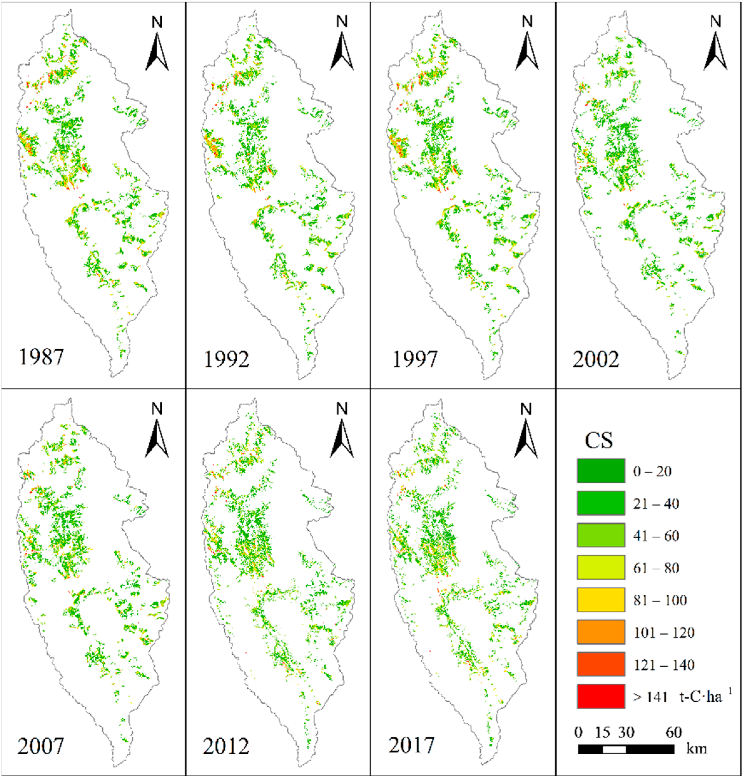
3.2. Mapping Carbon Storage

According to the model evaluation results, the 5-year interval change RF model with the highest accuracy was used to estimate the carbon storage change. The scatter plot of this estimation model is shown in Figure 7. The direct estimation result of the model is the 5-year interval change of carbon storage of Pinus densata in Shangri-La. The values of the carbon storage change for the six change periods are Δ CS 1 = CS 1992 CS 1987 , Δ CS 2 = CS 1997 CS 1992 , Δ CS 3 = CS 2002 CS 1997 , Δ CS 4 = CS 2007 CS 2002 , Δ CS 5 = CS 2012 CS 2007 and Δ CS 6 = CS 2017 CS 2012 .
The estimated carbon storage changes in the six periods are as follows: ΔCS1 = −53.327 × 10⁴ t, ΔCS2 = 13.887 × 10⁴ t, ΔCS3 = −94.041 × 10⁴ t, ΔCS4 = 14.602 × 10⁴ t, ΔCS5 = 20.869 × 10⁴ t, and ΔCS6 = 5.602 × 10⁴ t. A positive value indicates an increase in total carbon storage, and a negative value indicates a decrease in total carbon storage. The estimation results indicate that the carbon storage of Pinus densata in Shangri-La decreased in the periods 1987–1992 and 1997–2002 and increased in the remaining four periods.
In order to obtain carbon storage maps for each year, the published AGB estimates for each year from our group were used [63], which contain the aboveground biomass estimates of Pinus densata in Shangri-La for 1987, 1992, 1997, 2002, 2007, 2012, and 2017. These data were combined with the results of carbon storage change values estimated in this paper to calculate the total carbon storage values for each year. Firstly, the AGB of each year in the published study was converted to carbon storage by multiplying the carbon content coefficient (0.501) and the converted values were expressed as T1987, T1992, T1997, T2002, T2007, T2012, and T2017; then the carbon storage change values ΔCS1, ΔCS2, ΔCS3, ΔCS4, ΔCS5 and ΔCS6 were added to the conversion values of the smaller years in each change period in order to obtain the carbon storage values for the six years 1992, 1997, 2002, 2007, 2012 and 2017, respectively (e.g., CS 1992 = Δ CS 1 +   T 1987 ), and the carbon storage value for 1987 was obtained by subtracting ΔCS1 from T1992 ( CS 1992 = T 1987 Δ CS 1 ). The statistical results for carbon storage are shown in Table 6, and Figure 8 and Figure 9 (the spatial resolution is 30 m) were obtained by mapping the values of the carbon storage change for each period and each year according to the Pinus densata distribution range. The distribution range and area of Pinus densata are derived from Forest Manager Inventory (FMI) data.

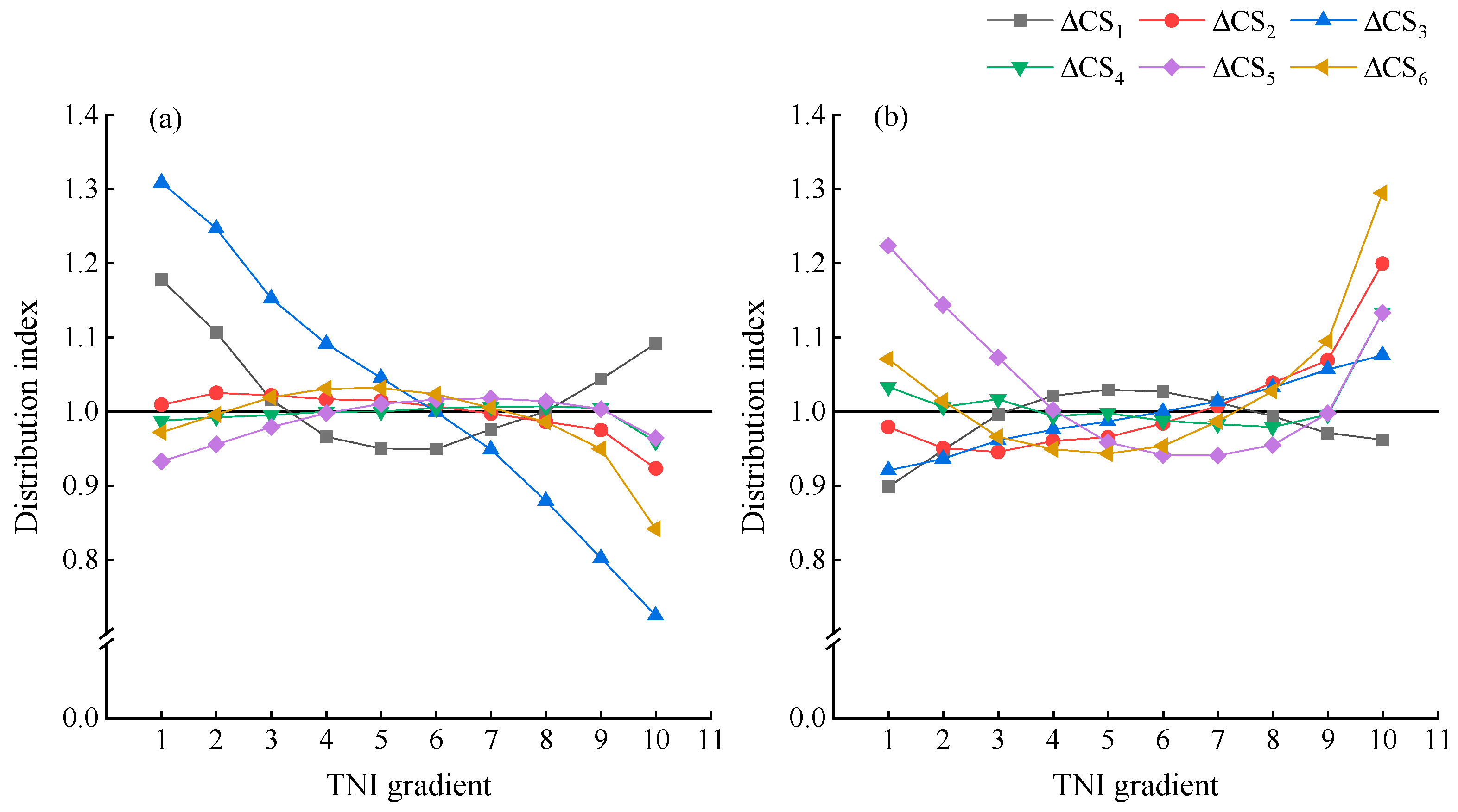
3.3. Spatial Distribution Characteristics for the Changes in Carbon Storage on Different TNI Gradients

In this study, the estimated changes in carbon storage were classified as increases (positive change values) and decreases (negative change values), and the TNI (0.30 to 0.93) was classified into ten levels from low to high using the natural breaks (Jenks) method: low (1–3), medium–low (4–5), medium–high (6–7), high (8–10). The DI was then calculated according to Equation (4) and used to explore the distribution of carbon storage changes along different TNI gradients. The distribution results are shown in Figure 10.
As can be seen from Figure 10, the increase and decrease in the carbon storage of Pinus densata in Shangri-La at each period have a certain regularity on the TNI gradient. The DI curve for ΔCS1(1987–1992) decreases and then rises when carbon storage increases (Figure 10a) with a dominant distribution in the low and high TNI gradients; the DI curve for ΔCS2 (1992–1997), ΔCS4 (2002–2007), ΔCS5 (2007–2012), and ΔCS6 (2012–2017) rises and then reduces with the dominant distribution areas of ΔCS2 being in the low and medium TNI gradients, and the dominant distribution areas of ΔCS4, ΔCS5, and ΔCS6 being concentrated in the medium–high TNI gradients; and ΔCS3 (1997–2002) reduces with the TNI gradient, and its dominant distribution area is in the low and medium–low gradients. The corresponding curve change period displays a decreasing trend when the carbon storage decreases (Figure 10b). Overall, the dominant distribution areas for each period when carbon storage increases are mainly found in the lower or middle TNI gradients, while the dominant distribution areas for each period when carbon storage decreases are found in all TNI gradients.

4. Discussion

In long time series data, the uncertainty of the historical data, due to the events that took place at the time being taken into account, cause some of the data to display large deviations in values, which are known as anomalies or outliers [64]. The stability of the model can be affected by outliers, and at the same time, the prediction accuracy of the model may be reduced, so the detection and handling of outliers is very important in the modelling process [65]. The sample plot data were screened twice in this study, the first time removing plots with an AGB of less than 1 t·ha−1 because they had an average diameter at breast height of less than 5 cm and an average tree height of less than 1.5 m. They are young forests, too low in canopy density, and poorly characterized by the appearance of the forest floor (similar to bare ground) on 30 m resolution imagery. Values exceeding the range of x ¯ ± 3 σ were selected for the second time using the Pauta criterion. By removing values that are too small and too large from the data in these two steps, respectively, the overall uncertainty of the data is reduced and the reliability of the data is improved.
The remote sensing-based estimation model is one of the main methods used in current carbon storage studies [7]. Based on the accumulation of ground survey data, the results of remote sensing estimation models are considered to have certain advantages and reliability in forest carbon storage studies. Time series images also provide an important basis for describing change [66]. The NFI and Landsat time series data over a 30-year period were combined to develop a dynamic model to study forest carbon storage in this paper. Although dynamic models based on change data are currently less commonly used in forestry, their advantages in terms of accuracy have been demonstrated [11,12]. In this study, although the effects of dynamic models and static models are not directly compared through experiments, we can refer to some of the existing studies related to forest carbon storage modelling in recent years [8,67,68]. The R2 of the remote sensing static models developed in these studies ranges from 0.64 to 0.73 as the highest value, while the R2 of the optimal model in this study is 0.87. Thus, the advantages of the dynamic model in terms of accuracy can be seen.
The DI is an area evaluation indicator. When the distribution curve is flatter, it indicates that the distribution of such changes deviates less from the standard distribution, and its adaptability to the terrain is wider [16]. In this study, the areas of increasing or decreasing Pinus densata carbon storages were calculated separately, and the main topography of these two areas was evaluated according to the DI. The results of this study demonstrate that the increase in carbon storage in the periods ΔCS4, ΔCS5, and ΔCS6 is much greater than the decrease, leading to an increase in total carbon storage from 2002 to 2017, which is related to the policy of “returning farmland to the forest” that has been implemented in Shangri-La since 2000. In the area of increasing carbon storage, the distribution curves of these three periods are relatively flat, showing a general adaptation to different levels of TNI and suggesting that the implementation of this government policy has led to the widespread planting of Pinus densata in Shangri-La, thus resulting in a more balanced topographic distribution of increasing carbon storage across the region.
Different TNI levels reflect different elevation and slope conditions, and the dominant distribution reflects the main topographic range of carbon storage changes. Although the dominant distribution of carbon storage changes over the TNI gradient can be clearly seen throughout a particular period of change, the six periods of change in carbon storage are more complex, and the distribution trends across the periods of change are not entirely consistent along the TNI gradient. What can be seen from the dominant distribution is that the regions where carbon storage increased are mainly located at low altitudes or on gently sloping terrain or both, as such terrain is conducive to artificial tending. In contrast, in regions with decreased carbon storage, the dominant distribution occurs across the TNI gradient, and the overall dominance of the terrain is not obvious, which is due to the randomicity of deforestation or forest destruction. In the past, TNI has not been applied to separate forest land class studies, but this study shows that its combination with the DI can be used to evaluate the increase and decrease effects of a single land type.
Some studies have suggested that human activities are the main driver of forest carbon [69], but as Shangri-La is a highland region with a low population density, the impact of human life on the surrounding forests is also relatively low, and it is environmental factors, including topography, that mainly impact forest carbon storage. Therefore, it is essential to consider topographic factors when studying forest carbon storage in this region. The results of this paper show that adding TNI to the dynamic model can reflect the topographic effect of the model and enable the improvement of the dynamic model accuracy, and by analyzing the distribution of forest carbon storage changes along the TNI gradient, it is possible to reveal the changes in forest carbon storage under different topographic conditions.
At present, the main approach to the study of historical forest dynamics is still based on the estimation of forest biomass or carbon storage over several single years, and the values of changes in different periods are calculated in order to derive forest dynamics results [70]. The level of periodic change in the forest can be estimated directly from models developed from interval change data, and due to the advantages of dynamic models in terms of accuracy, the resulting change values are estimated more precisely. Different dynamic models can be obtained for different types of change data. In this paper, we only compared two dynamic models for the 5-year interval change data and annual average change data, and more types of dynamic models are yet to be explored.
Although it was difficult to derive carbon storage results for a single year in this study without the support of carbon storage inventory data or graphs related to the study years, the results of this study demonstrate that the dynamic model is able to estimate the change in forest carbon storage and is well suited for the study of forest carbon storage change. Dynamic models are capable of quantitatively describing changes in specific properties, so they need not be limited to the field of forestry research but have the potential for application in other areas of natural or manufactured landscapes where regular variation exists. This study has so far only considered the influence of topographic factors, and there remains the possibility of other environmental factors, such as climate and soil, also influencing the model, which could be the next direction for future research.

5. Conclusions

In this study, the carbon storage dynamic model was developed based on NFI data and Landsat time series images over a 30-year period. PLSR, RF, and GBRT were used for modelling, and the accuracy of the two dynamic models was compared; then TNI, which represents topographic factors, was introduced into the model, and the distribution of carbon storage changes in Shangri-La on different TNI gradients was analyzed. The main conclusions are as follows: (1) the model effects of the non-parametric methods, RF and GBRT, are much better than those of the parametric method, PLSR, and the accuracy of the 5-year interval change model is better than that of the annual average change model; (2) TNI can improve the accuracy of the dynamic carbon storage estimation model, and the accuracy of the dynamic model with RF is the highest after adding TNI; (3) the dynamic model displays good performance regarding the estimation of carbon storage changes, and the results of the interval change model show that the total carbon storage of Pinus densata in Shangri-La decreased in 1987–1992 and 1997–2002, and increased in 1992–1997, 2002–2007, 2007–2012, and 2012–2017; and (4) the DI can be used to evaluate the main topography for the regions that display a change in Pinus densata carbon storage, the predominant topography in the regions of increasing carbon storage is that of low elevations or low slopes, or a combination of both conditions, while the topography in regions of decreasing carbon storage is more random. The results of this study can be used as a reference for forest carbon storage estimation using Landsat images in areas with complex topography.

Author Contributions

Y.L. participated in the data analysis and wrote the draft article, J.Z. helped with the idea and draft revision, R.B. helped with the data analysis, and D.X. and D.H. participated in the draft revision. All authors have read and agreed to the published version of the manuscript.

Funding

This research was funded by the National Natural Science Foundation of China (Nos. 31860207 and 32260390), and the “Young Top Talents” special project of the high-level talent training support program of Yunnan province, China, in 2020 (No. YNWR-QNBJ-2020-164).

Data Availability Statement

The data presented in this study are available on request from the corresponding author. The data are not publicly available due to the confidentiality of the NFI dataset.

Acknowledgments

We would like to thank the editor and anonymous reviewers for their comments, which helped improve the manuscript. We also would like to acknowledge all the others individuals who contributed to this paper.

Conflicts of Interest

The authors declare no conflict of interest.

References

  1. Shao, W.; Cai, J.; Wu, H.; Liu, J.; Zhang, H.; Huang, H. An Assessment of Carbon Storage in China’s Arboreal Forests. Forests 2017, 8, 110. [Google Scholar] [CrossRef] [Green Version]
  2. Solomon, S.D.; Qin, D.; Manning, M.; Chen, Z.; Miller, H.L. Climate Change 2007: The Physical Science Basis. In Working Group I Contribution to the Fourth Assessment Report of the IPCC; Cambridge University Press: Cambridge, UK, 2007. [Google Scholar]
  3. Luo, K. Spatial Pattern of Forest Carbon Storage in the Vertical and Horizontal Directions Based on HJ-CCD Remote Sensing Imagery. Remote Sens. 2019, 11, 788. [Google Scholar] [CrossRef] [Green Version]
  4. Li, T.; Li, M.-Y.; Tian, L. Dynamics of Carbon Storage and Its Drivers in Guangdong Province from 1979 to 2012. Forests 2021, 12, 1482. [Google Scholar] [CrossRef]
  5. Long, Y.; Jiang, F.G.; Sun, H.; Wang, T.H.; Zou, Q.; Chen, C.S. Estimating vegetation carbon storage based on optimal bandwidth selected from geographically weighted regression model in Shenzhen City. Acta Ecol. Sin. 2022, 42, 4933–4945. [Google Scholar]
  6. Zhang, P.P.; Li, Y.H.; Yin, H.R.; Chen, Q.T.; Dong, Q.D.; Zhu, L.Q. Spatio-temporal variation and dynamic simulation of ecosystem carbon storage in the north-south transitional zone of China. J. Nat. Resour. 2022, 37, 1183–1197. [Google Scholar] [CrossRef]
  7. Yan, E.; Lin, H.; Wang, G.; Sun, H. Improvement of Forest Carbon Estimation by Integration of Regression Modeling and Spectral Unmixing of Landsat Data. IEEE Geosci. Remote Sens. Lett. 2015, 12, 2003–2007. [Google Scholar]
  8. Safari, A.; Sohrabi, H.; Powell, S.; Shataee, S. A comparative assessment of multi-temporal Landsat 8 and machine learning algorithms for estimating aboveground carbon stock in coppice oak forests. Int. J. Remote Sens. 2017, 38, 6407–6432. [Google Scholar] [CrossRef]
  9. Sun, W.; Liu, X. Review on carbon storage estimation of forest ecosystem and applications in China. For. Ecosyst. 2019, 7, 4. [Google Scholar] [CrossRef] [Green Version]
  10. Gómez, C.; White, J.C.; Wulder, M.A. Characterizing the state and processes of change in a dynamic forest environment using hierarchical spatio-temporal segmentation. Remote Sens. Environ. 2011, 115, 1665–1679. [Google Scholar] [CrossRef]
  11. Gómez, C.; White, J.C.; Wulder, M.A.; Alejandro, P. Historical forest biomass dynamics modelled with Landsat spectral trajectories. ISPRS J. Photogramm. Remote Sens. 2014, 93, 14–28. [Google Scholar] [CrossRef] [Green Version]
  12. Zhang, J.; Lu, C.; Xu, H.; Wang, G. Estimating aboveground biomass of Pinus densata-dominated forests using Landsat time series and permanent sample plot data. J. For. Res. 2019, 30, 1689–1706. [Google Scholar] [CrossRef]
  13. Liu, C.; Zhang, L.; Li, F.; Jin, X. Spatial modeling of the carbon stock of forest trees in Heilongjiang Province, China. J. For. Res. 2014, 25, 269–280. [Google Scholar] [CrossRef]
  14. Oltean, G.S.; Comeau, P.G.; White, B. Linking the Depth-to-Water Topographic Index to Soil Moisture on Boreal Forest Sites in Alberta. For. Sci. 2016, 62, 154–165. [Google Scholar] [CrossRef]
  15. Deng, Y.; Chen, X.; Kheir, R.B. An Exploratory Procedure Defining a Local Topographic Index for Mountainous Vegetation Conditions. GIScience Remote Sens. 2007, 44, 383–401. [Google Scholar] [CrossRef]
  16. Wu, A.B.; Qin, Y.J.; Zhao, Y.X. Terrain composite index and its application in terrain gradient effect analysis of land use change: A case study of Taihang Hilly areas. Geogr. Geo. Inf. Sci. 2018, 34, 93–99+118. [Google Scholar]
  17. Wang, Q.; Yang, K.; Li, L.; Zhu, Y. Assessing the Terrain Gradient Effect of Landscape Ecological Risk in the Dianchi Lake Basin of China Using Geo-Information Tupu Method. Int. J. Environ. Res. Public Health 2022, 19, 9634. [Google Scholar] [CrossRef] [PubMed]
  18. Gong, W.; Wang, H.; Wang, X.; Fan, W.; Stott, P. Effect of terrain on landscape patterns and ecological effects by a gradient-based RS and GIS analysis. J. For. Res. 2017, 28, 1061–1072. [Google Scholar] [CrossRef]
  19. Zhao, Y.; Cao, J.; Zhang, X.; Zhang, M. Analyzing the characteristics of land use distribution in typical village transects at Chinese Loess Plateau based on topographical factors. Open Geosci. 2022, 14, 429–442. [Google Scholar] [CrossRef]
  20. Li, C.; Chen, D.; Wu, D.; Su, X. Design of an EIoT system for nature reserves: A case study in Shangri-La County, Yunnan Province, China. Int. J. Sustain. Dev. World Ecol. 2015, 22, 184–188. [Google Scholar] [CrossRef]
  21. Pan, J.; Wang, J.; Gao, F.; Liu, G. Quantitative estimation and influencing factors of ecosystem soil conservation in Shangri-La, China. Geocarto Int. 2022, 1–15. [Google Scholar] [CrossRef]
  22. Yu, Y.; Wang, J.; Liu, G.; Cheng, F. Forest Leaf Area Index Inversion Based on Landsat OLI Data in the Shangri-La City. J. Indian Soc. Remote Sens. 2019, 47, 967–976. [Google Scholar] [CrossRef]
  23. Chen, Y.; Wang, J.; Liu, G.; Yang, Y.; Liu, Z.; Deng, H. Hyperspectral Estimation Model of Forest Soil Organic Matter in Northwest Yunnan Province, China. Forests 2019, 10, 217. [Google Scholar] [CrossRef] [Green Version]
  24. Sun, X.L. Study on Biomass Estimation of Pinus Densata in Shangri-La Based on Landsat8-OLI. Master’s Thesis, Southwest Forestry University, Kunming, China, 2016. [Google Scholar]
  25. Yao, X.L.; Chen, H.L.; Zhao, X.; Guo, S.J. Weak link determination of anti-shock performance of shipboard equipments based on Pauta criterion. Chin. J. Ship Res. 2007, 2, 10–14. [Google Scholar]
  26. Xie, H.; Zhao, A.; Huang, S.; Han, J.; Liu, S.; Xu, X.; Luo, X.; Pan, H.; Du, Q.; Tong, X. Unsupervised Hyperspectral Remote Sensing Image Clustering Based on Adaptive Density. IEEE Geosci. Remote Sens. Lett. 2018, 15, 632–636. [Google Scholar] [CrossRef]
  27. LY/T 2988-2018; Guideline on Carbon Stock Accounting in Forest Ecosystem. State Forestry and Grassland Administration of China: Beijing, China, 2018; pp. 1–16.
  28. Chander, G.; Markham, B.L.; Helder, D.L. Summary of current radiometric calibration coefficients for Landsat MSS, TM, ETM+, and EO-1 ALI sensors. Remote Sens. Environ. 2009, 113, 893–903. [Google Scholar] [CrossRef]
  29. Yu, K.; Liu, S.; Zhao, Y. CPBAC: A quick atmospheric correction method using the topographic information. Remote Sens. Environ. 2016, 186, 262–274. [Google Scholar] [CrossRef]
  30. Nichol, J.; Hang, L.K.; Sing, W.M. Empirical correction of low Sun angle images in steeply sloping terrain: A slope-matching technique. Int. J. Remote Sens. 2006, 27, 629–635. [Google Scholar] [CrossRef]
  31. Zhang, J.; Pham, T.-T.-H.; Kalacska, M.; Turner, S. Using Landsat Thematic Mapper records to map land cover change and the impacts of reforestation programmes in the borderlands of southeast Yunnan, China: 1990–2010. Int. J. Appl. Earth Obs. Geoinf. 2014, 31, 25–36. [Google Scholar] [CrossRef]
  32. Carleer, A.P.; Wolff, E. Urban land cover multi-level region-based classification of VHR data by selecting relevant features. Int. J. Remote Sens. 2008, 27, 1035–1051. [Google Scholar] [CrossRef]
  33. Wang, W.; Jiang, Y.; Wang, G.; Guo, F.; Li, Z.; Liu, B. Multi-Scale LBP Texture Feature Learning Network for Remote Sensing Interpretation of Land Desertification. Remote Sens. 2022, 14, 3486. [Google Scholar] [CrossRef]
  34. Zhang, C.; Huang, C.; Li, H.; Liu, Q.; Li, J.; Bridhikitti, A.; Liu, G. Effect of Textural Features in Remote Sensed Data on Rubber Plantation Extraction at Different Levels of Spatial Resolution. Forests 2020, 11, 399. [Google Scholar] [CrossRef] [Green Version]
  35. Yuan, J.; Wang, D.; Li, R. Remote Sensing Image Segmentation by Combining Spectral and Texture Features. IEEE Trans. Geosci. Remote Sens. 2014, 52, 16–24. [Google Scholar] [CrossRef]
  36. Duan, M.; Song, X.; Liu, X.; Cui, D.; Zhang, X. Mapping the soil types combining multi-temporal remote sensing data with texture features. Comput. Electron. Agric. 2022, 200, 107230. [Google Scholar] [CrossRef]
  37. Rui, B.; Zhang, J.; Lu, C.; Chen, P. Estimating above-ground biomass of Pinus densata Mast. Using best slope temporal segmentation and Landsat time series. J. Appl. Remote Sens. 2021, 15, 024507. [Google Scholar]
  38. Powell, S.L.; Cohen, W.B.; Healey, S.P.; Kennedy, R.E.; Moisen, G.G.; Pierce, K.B.; Ohmann, J.L. Quantification of live aboveground forest biomass dynamics with Landsat time-series and field inventory data: A comparison of empirical modeling approaches. Remote Sens. Environ. 2010, 114, 1053–1068. [Google Scholar] [CrossRef]
  39. Wei, H.L.; Qi, Y.J. Analysis of grassland degradation of the Tibet Plateau and human driving forces based on remote sensing. Pratacultural Sci. 2016, 33, 2576–2586. [Google Scholar]
  40. Zhang, G.L. Spatial distribution characteristics of carbon storage of urban forests in Shanghai based on remote sensing estimation. Ecol. Environ. Sci. 2021, 30, 1777–1786. [Google Scholar]
  41. Yu, H.; Zeng, H.; Jiang, Z.Y. Study on Distribution Characteristics of Landscape Elements along the Terrain Gradient. Scientia Geogr. Sin. 2001, 1, 64–69. [Google Scholar]
  42. Emamian, A.; Rashki, A.; Kaskaoutis, D.G.; Gholami, A.; Opp, C.; Middleton, N. Assessing vegetation restoration potential under different land uses and climatic classes in northeast Iran. Ecol. Indic. 2021, 122, 107325. [Google Scholar] [CrossRef]
  43. Chen, L.D.; Yang, S.; Feng, X.M. Land use change characteristics along the terrain gradient and the spatial expanding analysis: A case study of Haidian District and Yanqing County, Beijing. Geogr. Res. 2008, 27, 1225–1234+1481. [Google Scholar]
  44. Huang, C.; Goward, S.N.; Schleeweis, K.; Thomas, N.; Masek, J.G.; Zhu, Z. Dynamics of national forests assessed using the Landsat record: Case studies in eastern United States. Remote Sens. Environ. 2009, 113, 1430–1442. [Google Scholar] [CrossRef]
  45. Lunetta, R.S.; Johnson, D.M.; Lyon, J.G.; Crotwell, J. Impacts of imagery temporal frequency on land-cover change detection monitoring. Remote Sens. Environ. 2004, 89, 444–454. [Google Scholar] [CrossRef]
  46. Yin, S.-L.; Zhang, X.-L.; Liu, S. Intrusion detection for capsule networks based on dual routing mechanism. Comput. Netw. 2021, 197, 108328. [Google Scholar] [CrossRef]
  47. Lian, Y.; Luo, J.; Xue, W.; Zuo, G.; Zhang, S. Cause-driven Streamflow Forecasting Framework Based on Linear Correlation Reconstruction and Long Short-term Memory. Water Resour. Manag. 2022, 36, 1661–1678. [Google Scholar] [CrossRef]
  48. Gregorutti, B.; Michel, B.; Saint-Pierre, P. Correlation and variable importance in random forests. Stat. Comput. 2017, 27, 659–678. [Google Scholar] [CrossRef] [Green Version]
  49. Zuur, A.F.; Ieno, E.N.; Elphick, C.S. A protocol for data exploration to avoid common statistical problems. Methods Ecol. Evol. 2010, 1, 3–14. [Google Scholar] [CrossRef]
  50. Farifteh, J.; Van der Meer, F.; Atzberger, C.; Carranza, E.J.M. Quantitative analysis of salt-affected soil reflectance spectra: A comparison of two adaptive methods (PLSR and ANN). Remote Sens. Environ. 2007, 110, 59–78. [Google Scholar] [CrossRef]
  51. Paul, G.; Kowalski, B.R. Partial least-squares regression: A tutorial. Anal. Chim. Acta 1986, 185, 1–17. [Google Scholar]
  52. Wold, S.; Sjöström, M.; Eriksson, L. PLS-regression: A basic tool of chemometrics. Chemom. Intell. Lab. Syst. 2001, 58, 109–130. [Google Scholar] [CrossRef]
  53. Song, G.Y. Research on Partial Least Squares Regression. Master’s Thesis, Zhejiang University, Hangzhou, China, 2009. [Google Scholar]
  54. Ryan, T.A., Jr.; Joiner, B.L. Minitab: A Statistical Computing System for Students and Researchers. Am. Stat. 1973, 27, 222–225. [Google Scholar] [CrossRef]
  55. Friedman, J.H. Greedy Function Approximation: A Gradient Boosting Machine. Ann. Stat. 2001, 29, 1189–1232. [Google Scholar] [CrossRef]
  56. Friedman, J.H. Stochastic gradient boosting. Comput. Stat. Data Anal. 2002, 38, 367–378. [Google Scholar] [CrossRef]
  57. Lawrence, R.; Bunn, A.; Powell, S.; Zambon, M. Classification of remotely sensed imagery using stochastic gradient boosting as a refinement of classification tree analysis. Remote Sens. Environ. 2004, 90, 331–336. [Google Scholar] [CrossRef]
  58. Wang, L.; Zhang, Y.; Yao, Y.; Xiao, Z.; Shang, K.; Guo, X.; Yang, J.; Xue, S.; Wang, J. GBRT-Based Estimation of Terrestrial Latent Heat Flux in the Haihe River Basin from Satellite and Reanalysis Datasets. Remote Sens. 2021, 13, 1054. [Google Scholar] [CrossRef]
  59. Breiman, L. Random Forests. Mach. Learn. 2001, 45, 5–32. [Google Scholar] [CrossRef] [Green Version]
  60. van der Meer, D.; Hoekstra, P.J.; van Donkelaar, M.; Bralten, J.; Oosterlaan, J.; Heslenfeld, D.; Faraone, S.V.; Franke, B.; Buitelaar, J.K.; Hartman, C.A. Predicting attention-deficit/hyperactivity disorder severity from psychosocial stress and stress-response genes: A random forest regression approach. Transl. Psychiatry 2017, 7, e1145. [Google Scholar] [CrossRef] [Green Version]
  61. Sun, J.; Zhong, G.; Huang, K.; Dong, J. Banzhaf random forests: Cooperative game theory based random forests with consistency. Neural Netw. 2018, 106, 20–29. [Google Scholar] [CrossRef]
  62. Wang, X.; Liu, T.; Zheng, X.; Peng, H.; Xin, J.; Zhang, B. Short-term prediction of groundwater level using improved random forest regression with a combination of random features. Appl. Water Sci. 2018, 8, 125. [Google Scholar] [CrossRef] [Green Version]
  63. Xu, D.; Zhang, J.; Bao, R.; Liao, Y.; Han, D.; Liu, Q.; Cheng, T. Temporal and Spatial Variation of Aboveground Biomass of Pinus densata and Its Drivers in Shangri-La, CHINA. Int. J. Environ. Res. Public Health 2021, 19, 400. [Google Scholar] [CrossRef]
  64. Li, J.; Sun, G.Z.; Xu, Y.L. Application and anomaly detection of Application and anomaly detection of predictive model based on time series predictive model based on time series. Comput. Aided Eng. 2006, 15, 49–54+84. [Google Scholar]
  65. Ranjan, K.G.; Tripathy, D.S.; Prusty, B.R.; Jena, D. An improved sliding window prediction-based outlier detection and correction for volatile time-series. Int. J. Numer. Model. Electron. Netw. Devices Fields 2021, 34, e2816. [Google Scholar] [CrossRef]
  66. Goodwin, N.R.; Coops, N.C.; Wulder, M.A.; Gillanders, S.; Schroeder, T.A.; Nelson, T. Estimation of insect infestation dynamics using a temporal sequence of Landsat data. Remote Sens. Environ. 2008, 112, 3680–3689. [Google Scholar] [CrossRef]
  67. Zhang, M.; Du, H.; Zhou, G.; Li, X.; Mao, F.; Dong, L.; Zheng, J.; Liu, H.; Huang, Z.; He, S. Estimating Forest Aboveground Carbon Storage in Hang-Jia-Hu Using Landsat TM/OLI Data and Random Forest Model. Forests 2019, 10, 1004. [Google Scholar] [CrossRef] [Green Version]
  68. Zhang, X.; Sun, Y.; Jia, W.; Wang, F.; Guo, H.; Ao, Z. Research on the Temporal and Spatial Distributions of Standing Wood Carbon Storage Based on Remote Sensing Images and Local Models. Forests 2022, 13, 346. [Google Scholar] [CrossRef]
  69. Pyles, M.V.; Magnago, L.F.S.; Maia, V.A.; Pinho, B.X.; Pitta, G.; de Gasper, A.L.; Vibrans, A.C.; Santos, R.M.D.; van Den Berg, E.; Lima, R.A. Human impacts as the main driver of tropical forest carbon. Sci. Adv. 2022, 8, eabl7968. [Google Scholar] [CrossRef]
  70. Nguyen, T.H.; Jones, S.D.; Soto-Berelov, M.; Haywood, A.; Hislop, S. Monitoring aboveground forest biomass dynamics over three decades using Landsat time-series and single-date inventory data. Int. J. Appl. Earth Obs. Geoinf. 2020, 84, 101952. [Google Scholar] [CrossRef]
Figure 1. Study area and sample plots.
Remotesensing 14 06244 g001
Figure 2. Flow chart of the main content in this study.
Remotesensing 14 06244 g002
Figure 3. Sample plot data records by year: different colors represent sample plots with different locations (different numbered sample plots).
Remotesensing 14 06244 g003
Figure 4. Boxplots of basic information on sample plots by year.
Remotesensing 14 06244 g004
Figure 5. Changes in model indicators after adding TNI: positive values on the right side of the y-axis represent an increase, and negative values on the left side of the y-axis represent a decrease.
Remotesensing 14 06244 g005
Figure 6. Confidence intervals (95%) of the accuracy evaluation indicators for different models: (a) the model of 5-year interval change before adding TNI; (b) the model of 5-year interval change after adding TNI; (c) the model of annual average change model before adding TNI; and (d) the model of annual average change after adding TNI.
Remotesensing 14 06244 g006
Figure 7. Scatter plot of the estimation model.
Remotesensing 14 06244 g007
Figure 8. Change values for carbon storage for six time periods.
Remotesensing 14 06244 g008
Figure 9. Carbon storage values for seven years.
Remotesensing 14 06244 g009
Figure 10. Distribution of increased carbon storage (a) and decreased carbon storage (b) on the TNI gradient.
Remotesensing 14 06244 g010
Table 1. Landsat time-series of imagery used in the study.
YearLandsat/SensorPath/RowImage Acquisition Date
19875/TM132/04030 December 1987
5/TM132/04130 December 1987
5/TM131/04123 December 1987
19925/TM132/0417 November 1991
5/TM132/0407 November 1991
5/TM131/04116 November 1991
19975/TM132/0417 November 1997
5/TM132/0406 October 1997
5/TM131/04116 November 1997
20025/TM132/0415 January 2002
5/TM132/0405 January 2002
5/TM131/04129 October 2002
20075/TM132/04115 October 2006
5/TM132/0403 January 2007
5/TM131/0411 March 2007
20125/TM132/04113 October 2011
5/TM132/04014 January 2011
5/TM131/0417 January 2011
20178/OLI132/04116 December 2017
8/OLI132/04016 December 2017
8/OLI131/04125 December 2017
Table 2. Extracted remote sensing feature information.
CategoriesInformation on Remote Sensing Characteristics
Spectral featuresOriginal bandsB1; B2; B3; B4; B5; B7
Vegetation indices [37] NDVI = ( B 4 B 3 ) / ( B 4 + B 3 ) ;
ND 32 = ( B 3 B 2 ) / ( B 3 + B 2 ) ;
ND 54 = ( B 5 B 4 ) / ( B 5 + B 4 ) ;
ND 53 = ( B 5 B 3 ) / ( B 5 + B 3 ) ;
ND 57 = ( B 5 B 7 ) / ( B 5 + B 7 ) ;
ND 452 = ( B 4 + B 5 B 2 ) / ( B 4 + B 5 + B 2 ) ;
DVI = B 4 B 3 ; RVI = B 4 / B 3 ;
ARVI = ( B 4 ( 2 B 3 B 1 ) ) / ( B 4 + ( 2 B 3 B 1 ) )
EVI = 2.5 × B 4 B 3 B 4 + 6 B 3 7.5 B 1 + 1 ;
Band combination [12] B 4 / B 2 ; B 5 / B 3 ; B 5 / B 4 ;
B 5 / B 7 ; B 7 / B 3 ; B 4 × ( B 3 / B 7 )
Image enhancement [38,39] Albedo = B 1 + B 2 + B 3 + B 4 + B 5 + B 7 ;
VIS 123 = B 1 + B 2 + B 3 ; MID = B 5 + B 7 ;
FVC = EVI EVI min EVI max EVI min ;
Principal component analysis (PCA1, PCA2, PCA3, PCA4, PCA5, PCA7);
Tasseled cap transform (TCT1, TCT2, TCT3)
Texture featuresGrey level
co-occurrence matrix [34]
Homogeneity (HO); Dissimilarity (DI);
Mean (ME); Angular second moment (SM);
Entropy (EN); Correlation (CC);
Variance (VA); Contrast (CO)
Filtering of probabilistic
statistics [40]
Skewness (SK)
Where B1 is the blue band, B2 is the green band, B3 is the red band, B4 is the near-infrared band, B5 is the shortwave infrared-1 band, and B7 is the shortwave infrared-2 band.
Table 3. Results of remote sensing feature screening.
Change TypeRemote Sensing Features
5-year interval change B 4 × ( B 3 / B 7 ) , B 5 / B 4 , PCA2, FVC, PCA4, R9B1EN, R17B7CO, R5B4SM
Annual average changeR3B3VA, R15B5VA, R17B1VA, R9B4HO, R15B5ME, DVI, PCA2, EVI, B 4 × ( B 3 / B 7 ) , B 7 / B 3
The expression of the texture features is “RXBYTT”, RX is the size of the texture window, BY is a certain single band of the image, and TT is the abbreviation of a certain texture feature.
Table 4. Comparison of modelling results.
Change TypeModelFittingValidation
R2RMSE/t-C·ha−1MAE/t-C·ha−1
5-year interval changePLSR0.189.619.09
GBRT0.814.582.51
RF0.854.091.83
PLSRTNI0.189.508.36
GBRTTNI0.834.242.43
RFTNI0.873.821.78
Annual average changePLSR0.231.831.64
GBRT0.800.940.45
RF0.830.870.36
PLSRTNI0.251.821.67
GBRTTNI0.820.890.41
RFTNI0.840.860.35
PLSR TNI, GBRTTNI, and RFTNI in the table indicate the PLSR model, GBRT model, and RF model after adding TNI, respectively.
Table 5. Error indicator for the adjusted annual average change.
Change TypeModelFittingValidation
RMSE/t-C·ha−1MAE /t-C·ha−1
Annual average changePLSR9.168.2
GBRT4.692.25
RF4.371.8
PLSRTNI9.0758.35
GBRTTNI4.4652.05
RFTNI4.2951.75
Table 6. Statistics of Pinus densata carbon storage.
YearArea of Pinus densata (ha)Total CS
(Million Tons)
Average CS
(t-C·ha−1)
1987171560.285.3030.91
1992171560.284.2424.69
1997170589.864.7727.97
2002170589.863.12 18.30
2007174179.373.9922.93
2012174213.124.0323.12
2017184815.843.80 20.53
Publisher’s Note: MDPI stays neutral with regard to jurisdictional claims in published maps and institutional affiliations.

