Hyperspectral Video Target Tracking Based on Deep Edge Convolution Feature and Improved Context Filter

Abstract

To address the problem that the performance of hyperspectral target tracking will be degraded when facing background clutter, this paper proposes a novel hyperspectral target tracking algorithm based on the deep edge convolution feature (DECF) and an improved context filter (ICF). DECF is a fusion feature via deep features convolving 3D edge features, which makes targets easier to distinguish under complex backgrounds. In order to reduce background clutter interference, an ICF is proposed. The ICF selects eight neighborhoods around the target as the context areas. Then the first four areas that have a greater interference in the context areas are regarded as negative samples to train the ICF. To reduce the tracking drift caused by target deformation, an adaptive scale estimation module, named the region proposal module, is proposed for the adaptive estimation of the target box. Experimental results show that the proposed algorithm has satisfactory tracking performance against background clutter challenges.

1. Introduction

As an important branch of computer vision, target tracking [1,2,3,4] is widely used in pedestrian monitoring [5,6], robot navigation [7,8], regional control [9,10], and other fields. The target tracking algorithm estimates the state of the target in each frame after giving the position and size of the target in the video sequence’s first frame. Most of target tracking methods based on visible light videos use the shape, appearance, and color information to track the target. However, when the color of the target and the background color are similar, how to accurately and robustly track the moving target is a challenge.

Compared to visible images, hyperspectral images (HSIs) [11,12] contain not only spatial but also spectral information about the target, so it has a wide range of applications in the fields of ground target recognition [13] and resource exploration [14]. Due to the large data scale of HSIs, it is difficult for traditional equipment to obtain hyperspectral videos (HSVs). The development of snapshot hyperspectral sensors provides a basis for us to use HSVs to track targets. Recently, Uzkent et al. [15] proposed a deep kernel correlation filter (DeepHKCF) to convert the hyperspectral image to a pseudo-color image, thereby obtaining the depth features of the image, ignoring the role of the spectrum. Qian et al. [16] proposed a hyperspectral target tracking method based on convolutional networks (CNHT), which only selects small cubes in the target area to train convolutional filters, ignoring the band correlation. In the HSVs, the usage of spectral information can improve the discrimination of targets, Xiong et al. [17] proposed a material-based hyperspectral target tracking method (MHT) that uses multidimensional gradient histograms to obtain spatial and spectral features, but it is difficult to maintain robustness when the background clutter is strong. Subsequently, Zhang et al. [18] adopted a variety of features for tracking, which caused tracking drift in the face of deformation due to the lack of a corresponding scale estimation strategy. However, the above trackers do not have corresponding strategies to deal with the interference of background clutter. Consequently, we optimize the traditional context-aware correlation filter (CACF) and propose a novel improved context filter (ICF) against the background clutter challenge.

In this paper, we propose a depth and convolution hyperspectral video tracker (DC-HVT) by using the deep edge convolution feature (DECF) and ICF for hyperspectral video target tracking. DC-HVT is based on the traditional correlation filtering framework, and the whole framework includes three parts: feature extraction, correlation filtering, and regression. The feature extraction part can be divided into a depth feature branch and a 3D edge feature branch. In the depth feature branch, the HSIs are dimensionality-reduced by principal components analysis (PCA) [19,20], and the results are fed into a pretrained ResNet50 [21] network to extract depth features. In the 3D edge feature branch, the spatial-spectral features of HSIs are extracted without destroying the overall structural information. Features of the two branches are convolutionally fused to obtain a more discriminative DECF. In the correlation filtering part, the adaptive weight is used to suppress the background clutter and increase the accuracy of the target localization. In the regression section, a region proposal module (RPM) is utilized to generate the rectangle boxes of target.

Following are the four primary contributions of this paper.

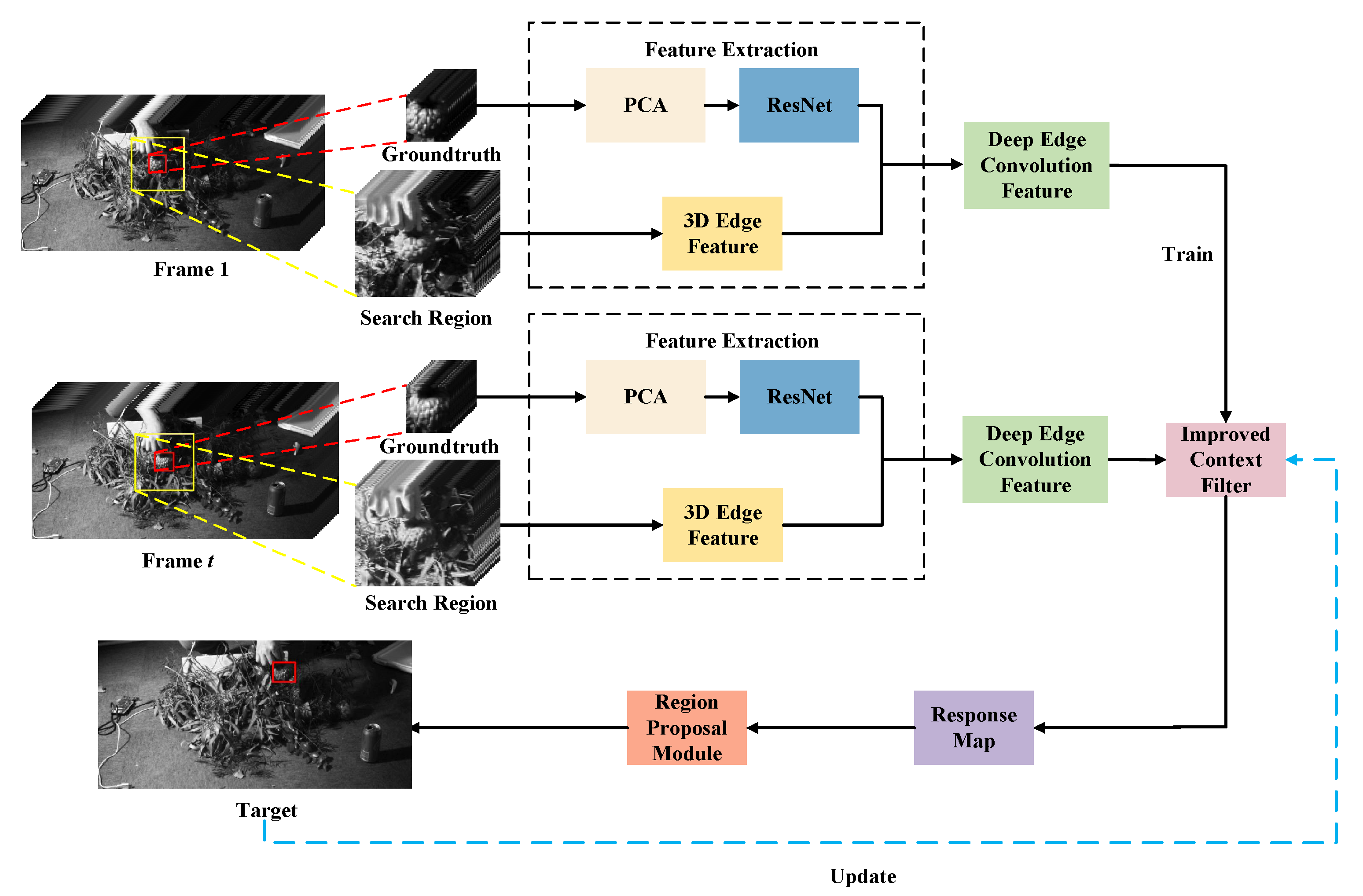
• We propose a 3D edge feature-extraction method. The three directional edge features are fused with directional adaptive weights to extract a 3D matrix, which enhances the edge information and contains spatial-spectral features.
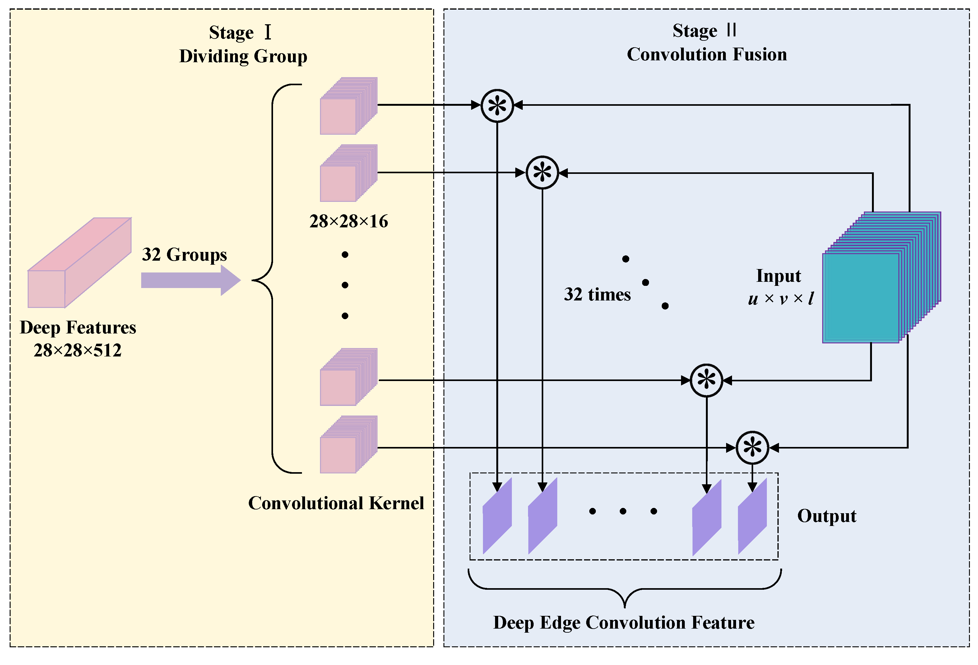
• We first used a novel convolution fusion feature named DECF, which is obtained by convolving the grouped depth features with the 3D edge features. DECF greatly preserves semantic and spatial-spectral information and makes the target more discriminative.
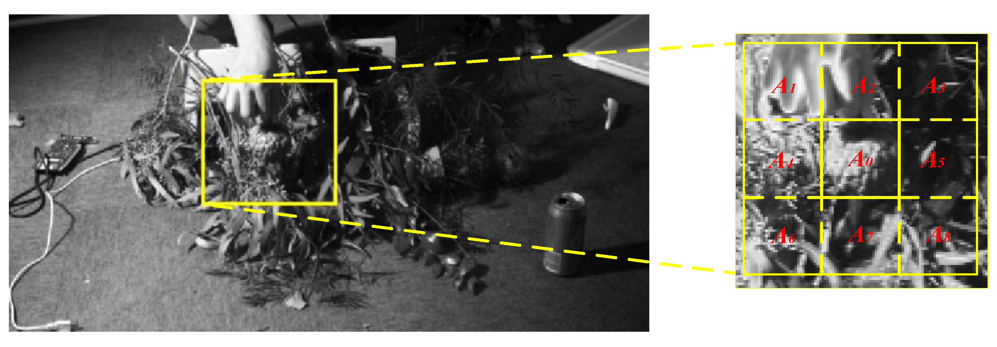
• An ICF is first proposed. First, eight influence factors are calculated in the context areas. Secondly, four areas corresponding to the first four influence factors are regarded as negative samples to train context filter. At last, adaptive weights calculated by four influence factors are used to suppress background clutter.
• Inspired by the region proposal network (RPN), this paper proposes a new adaptive scale estimation method named RPM. The estimation of the target box is achieved by adjusting the length and width of the target box by using RPM.

The rest of this research paper is organized as follows: Section 2 provides an overview of the related work. Section 3 describes the proposed approach. Section 4 presents the experiments for validating and analyzing the proposed framework. Section 5 discusses the conclusions drawn from this research.

2. Related Work

Our proposed DC-HVT can be divided into three parts, including feature extraction, correlation filtering-based trackers (CF trackers), and scale estimation. We reviewed the related methods that are relevant to these three parts as follows.

2.1. Feature Extraction

In order to fully extract the spatial-spectral features of HSIs, researchers have proposed various spatial-spectral feature extraction methods. Traditional manual features are typically represented by texture features and shape features, such as Gabor features [22], local binary pattern (LBP) features [23], and morphological profile features [24]. Zhu et al. [25] used 3D Gabor features to extract HSIs features from three angles for fusion, but this feature is only applicable to small samples. Li et al. [26] oriented to the rotation-invariant texture structure of HSIs local spatial information, and applied LBP to HSI feature extraction for the first time. This attempt yielded satisfactory results. In addition, feature-extraction methods based on LBP and sparse representation have also made progress. For example, Tu et al. [27] proposed a hyperspectral image classification method that combines LBP with a joint sparse representation classifier in order to fully utilize the texture features of images. This method improves the classification accuracy of hyperspectral images. With the development of deep learning [28,29], many computer vision works have made breakthroughs, and deep learning techniques have been widely used in HSIs. In the early days, Chen et al. [30] proposed a deep belief network, but it needed to represent the spatial information as vectors before training, and thus could not extract spatial information effectively. He et al. [31] built a 3D convolutional neural network (CNN) in order to extract the spectral and spatial information of HSIs at the same time, but the CNN model needs to convolve a fixed-sized region and cannot fully adapt to geometric changes.

2.2. CF Trackers

CF was first applied in the field of target detection. In 2010, Bolme et al. [32] proposed the minimum output sum of squared error (MOSSE) algorithm, which first used CF for video target tracking. Due to the small number of training samples in the MOSSE algorithm, it is easy to produce problems such as overfitting. For this reason, Henriques et al. [33] proposed a tracking-by-detection model, which uses a single grayscale feature [34] and does not adapt well to complex environments. Based on this, Henriques et al. [35] improved the single channel feature to a multichannel gradient histogram feature. This algorithm uses image gradients to improve the tracking accuracy. However, it brings boundary effects. To overcome this problem, Galoogahi et al. [36] expanded the training sample area to reduce the boundary effects. Danelljan et al. [37] introduced spatial regularization in spatially regularized discriminative correlation filters (SRDCF) to penalize boundary regions. Different from SRDCF, Mueller et al. [38] proposed a CACF, which uses the target context information as negative samples for filter training. But the performance of this method is restricted by the context area including four image patches.

2.3. Scale Estimation

Because CF usually uses a fixed-size window, it is easy to generate tracking drift when the target size changes. In order to solve this problem, Li et al. [39] used bounding boxes with multiple scales to match the target region in the previous frame and selected the bounding box with the highest similarity. Martin et al. [40] added a one-dimensional scale filter to the position filter to perform target localization and scale estimation respectively, but this method increased the computation complexity. Danelljan et al. [41] reduced the computational effort by using dimensionality reduction operation and QR decomposition. With the advancement of deep learning, Bertinetto et al. [42] pioneered the application of Siamese networks to track target and used, proposing the use of fully convolutional Siamese networks (SiamFC) to calculate the similarity between the template and the search region to achieve better performance in target tracking. However, SiamFC does not use regression to adjust the scale of the target box and requires multiscale testing to estimate the box’s size. To solve this problem, Li et al. [43,44] proposed the Siamese RPN model, which can better adapt to the scale changes of the tracked target.

3. Proposed Approach

To address the problems of degraded tracking accuracy and tracking drift under background clutter, DC-HVT is proposed in this paper. The proposed tracking framework is summarized in Figure 1. In frame 1, we selected the ground truth and search region manually. The frame 1 is used to train the template. PCA and ResNet are used to extract deep features of ground truth. Linear space scale theory [45,46,47] is used to extract 3D edge features of search region. In order to get the feature that contain more information, we convolved the above two features to get DECF. ICF is used to suppress the tracking drift caused by the background clutter. After ICF, we can get a response map to locate the target. RPM is used to adapt to the change of size during the movement of the target. After predicting the location and scale of the target in the next frame, the parameters of the ICF are updated. Therefore, DC-HVT maintains a good tracking performance against background clutter challenge.

3.1. PCA Dimensionality Reduction

The input of the pretrained ResNet50 is usually a one-band grayscale image or a three-band RGB image. Because the HSIs we used have 16 bands, the 16-band HSIs cannot be directly input into the network. So PCA [19,20,48] is used to reduce experimental HSIs with 16 bands to single-band images to meet the input requirements of the network.

Let X be the data sample such that $X=(x_1,x_2,x_3,\dots ,x_p)$, $x_i\in {\mathbb{R}}^{p\times l}$, p represents the pixels of HSIs, and l represents the bands of HSIs, the value of l is 16. We have

$$\psi =x_i-\overline{X}$$

(1)

where $\psi$ is the matrix after decentralization. $\overline{X}$ is the average pixel value for each band. Furthermore, a covariance matrix K, having significant location information, is constructed as

$$K=\frac{1}{p-1}\sum _{i=1}^p\psi {\psi }^T,$$

(2)

where the superscript T denotes the transpose operation. Furthermore, through the eigenvalue decomposition, the eigenvalues of K and the corresponding eigenvectors are obtained. We have

$$K\nu =\tau \nu$$

(3)

where $\nu$ represents the eigenvector, $\tau$ represents the eigenvalue. Then eigenvalues are sorted to get the largest eigenvalue ${\tau }_{max}$ and the corresponding eigenvector ${\nu }_{max}$, X is dimensionality reduced as

$$X_p={\nu }_{max}X,$$

(4)

where $X_p$ is the matrix after dimensionality reduction. As shown in Figure 2, after the dimension reduction of PCA, the amount of HSI data is reduced and becomes an image of one band.

3.2. Deep Features

ResNet [21] adopts identity connection, which cleverly skips the influence of the deep network weights, to achieve constant mapping [49]. The ResNet structure not only speeds up the training, but also ensures that the training accuracy is not affected by the increase in network depth. It also alleviates the problem of network degradation.

In this paper, ResNet50 is used to extract the deep features from the HSVs. The architecture constitutes of 50 layers, including 49 convolutional layers and one fully connected layer. The first stage facilitates input preprocessing, and the next four stages consist of bottlenecks, with convolutional units 2, 3, 4, and 5, respectively consisting of 3, 4, 6, and 3 bottlenecks.

In the field of target tracking, the spatial information is used to achieve accurate target localization, while the semantic information contained in deep features can enhance the robustness of the tracking algorithm. The spatial information is already provided by 3D edge features mentioned in Section 3.3. The deep features, extracted by res3d_branch2c in the pretrained ResNet50 network, are used to make up for the lack of semantic information.

$X_p$ is the input of ResNet50, and E is the feature extracted by ResNet50. Figure 3 shows the first 128 channels of deep features obtained by the experiment. It may be noted that the size of deep features is $m\times n\times r$. m represents the row of the deep features, n represents the column of the deep features, r is the number of channels. Our proposed algorithm uses the deep features extracted by res3d_branch2c, so the output feature’s size of this layer is $28\times 28\times 512$.

Figure 3 shows the first 128 channels of deep features. Because of the lack of spatial information, the target and background cannot be distinguished in Figure 3.

3.3. 3D Edge Features

As described earlier, HSIs are a three-dimensional cube consisting of two spatial dimensions and a spectral dimension. The feature-extraction methods based on RGB [50] images need to operate the bands of HSIs independently, which ignores the relationship between bands. Moreover, HSIs have many bands and a large amount of data, so using CNN [51] for feature extraction requires a large amount of computation.

HSIs are not only a three-dimensional data cube but also a three-dimensional discrete function, so the problem of obtaining the gradient of HSIs in three directions can be solved by obtaining partial derivatives for the three-dimensional discrete function. We use the derivative of the image to represent the gradient. In the spatial direction, the edge of the target is more obvious when the absolute value of the gradient increases [52,53], which facilitates target location. In the spectral direction, the target spectral curve is different from the background spectral curve, which can be observed by derivative differences. Therefore, when the target and the background are similar in space, the derivative differences of the spectral direction contribute to distinguish the target from the background. Hence, three-dimensional feature-extraction techniques are required. According to the linear scale space theory [45,46,47], any derivative of scale space can be computed by using convolution of the Gaussian kernel’s derivative. Hence, the derivative of HSIs in each direction can be obtained by solving the derivative of the Gaussian function in the corresponding direction.

In a 3D HSIs image, the Gaussian function can be expressed as

$$G\left(x,y,z\right)={\left(\frac{1}{\sqrt{2\pi }\sigma }\right)}^3{e}^{-\frac{x^2+y^2+z^2}{2{\sigma }^2}},\forall x,y,z\in W,$$

(5)

where x and y represent the spatial dimensions, z denotes the spectral dimension, $\sigma$ denotes the standard deviation of the normal distribution, and W denotes $w\times w\times w$ window. The first order partial derivatives of the Gaussian function with respect to x, y and z, respectively denoted as $\frac{\partial G\left(x,y,z\right)}{\partial x}$, $\frac{\partial G\left(x,y,z\right)}{\partial y}$, $\frac{\partial G\left(x,y,z\right)}{\partial z}$, are given as

$$\left\{\begin{array}{c}\hfill \frac{\partial G\left(x,y,z\right)}{\partial x}={\left(\frac{1}{\sqrt{2\pi }\sigma }\right)}^3{e}^{-\frac{x^2+y^2+z^2}{2{\sigma }^2}}\left(-\frac{x}{{\sigma }^2}\right)=-\frac{x}{{\left(\sqrt{2\pi }\right)}^3{\sigma }^5}{e}^{-\frac{x^2+y^2+z^2}{2{\sigma }^2}}\hfill \\ \hfill \frac{\partial G\left(x,y,z\right)}{\partial y}={\left(\frac{1}{\sqrt{2\pi }\sigma }\right)}^3{e}^{-\frac{x^2+y^2+z^2}{2{\sigma }^2}}\left(-\frac{y}{{\sigma }^2}\right)=-\frac{y}{{\left(\sqrt{2\pi }\right)}^3{\sigma }^5}{e}^{-\frac{x^2+y^2+z^2}{2{\sigma }^2}}\hfill \\ \hfill \frac{\partial G\left(x,y,z\right)}{\partial z}={\left(\frac{1}{\sqrt{2\pi }\sigma }\right)}^3{e}^{-\frac{x^2+y^2+z^2}{2{\sigma }^2}}\left(-\frac{z}{{\sigma }^2}\right)=-\frac{z}{{\left(\sqrt{2\pi }\right)}^3{\sigma }^5}{e}^{-\frac{x^2+y^2+z^2}{2{\sigma }^2}}.\hfill \end{array}\right.$$

(6)

In this paper, the search area for HSIs are denoted by H, $H\in {\mathbb{R}}^{u\times v\times l}$. u and v represent the width and height of the search region, respectively, and l denotes the number of bands. The first-order partial derivatives of H on $x,y,z$, respectively denoted as $I_x,I_y,I_z$, are given as

$$\left\{\begin{array}{c}{I}_x=H\left(x,y,z\right)\ast \frac{\partial G\left(x,y,z\right)}{\partial x}=H\left(x,y,z\right)\ast -\frac{x}{{\left(\sqrt{2\pi }\right)}^3{\sigma }^5}{e}^{-\frac{x^2+y^2+z^2}{2{\sigma }^2}}\\ I_y=H\left(x,y,z\right)\ast \frac{\partial G\left(x,y,z\right)}{\partial y}=H\left(x,y,z\right)\ast -\frac{y}{{\left(\sqrt{2\pi }\right)}^3{\sigma }^5}{e}^{-\frac{x^2+y^2+z^2}{2{\sigma }^2}}\\ I_z=H\left(x,y,z\right)\ast \frac{\partial G\left(x,y,z\right)}{\partial z}=H\left(x,y,z\right)\ast -\frac{z}{{\left(\sqrt{2\pi }\right)}^3{\sigma }^5}{e}^{-\frac{x^2+y^2+z^2}{2{\sigma }^2}},\end{array}\right.$$

(7)

where ∗ denotes convolution. The first-order derivative of the Gaussian function is employed to obtain the edge detection results in three directions. As the edge features in different directions have different effects on the image, fusion using simple weighted averaging or usage of static (nonadaptive) weights results in blurred edges.

This paper proposes a method to determine the fusion weights based on the change in the derivative value. The derivative of the image means the gradient of the image. The larger the absolute value of the gradient is, the more obvious the edge of the target is [52,53], which is convenient for locating the target. The gradient in the spectral direction represents the differences between adjacent bands, and it will be helpful to identify the target when the target and the background are similar in space. Therefore, by calculating the sum of the derivatives of each pixel in the direction of the edge, the proportion of the derivatives along different edge directions can be obtained. These proportions are used as weights for the corresponding edges for realising adaptive fusion of the image features. The adaptive weights can use the adjustable value when the background clutter changes. Figure 4 shows the distribution of a central pixel point and surrounding pixels within $I_x$, $I_y,I_z$ in the HSIs.

Taking a 3 × 3 × 3 region of the HSIs as an example, let the pixel locations in the center of the region within $I_x,I_y,I_z$ have the values $D_{xc},D_{yc},D_{zc}$. Let the value of the pixel point in the direction $D_{xc}$ within $I_x$ be $D_{xi}$. It may be noted that $D_{xc}^{{}^{\prime }}$ is defined as the sum of the values of the pixel points in the $I_x$ matrix that traverses the centre of the image. Similarly, $D_{yc}^{{}^{\prime }}$ and $D_{zc}^{{}^{\prime }}$ can also be obtained. Hence, $D_{xc}^{{}^{\prime }}$, $D_{yc}^{{}^{\prime }}$ and $D_{zc}^{{}^{\prime }}$ are computed as

$$D_{xc}^{{}^{\prime }}=\sum _{i=1}^{26}{D}_{xi}$$

(8)

$$D_{yc}^{{}^{\prime }}=\sum _{i=1}^{26}{D}_{yi}$$

(9)

$$D_{zc}^{{}^{\prime }}=\sum _{i=1}^{26}{D}_{zi}.$$

(10)

This weight is related to a cube with a size of 3 × 3 × 3 centered on the pixel. Except for the center pixel where the weight needs be calculated, there are still 26 pixels around the center pixel in 3D space. Therefore, the upper limit of the summation sign is set to 26. It may be noted that toward the edges of the matrix, the neighborhood values are subjected to a complementary 0 operation. Then, the adaptive weights of the edge features in different directions are given as

$$\varphi =\frac{D_{xc}^{{}^{\prime }}}{D_{xc}^{{}^{\prime }}+D_{yc}^{{}^{\prime }}+D_{zc}^{{}^{\prime }}}$$

(11)

$$\phi =\frac{D_{yc}^{{}^{\prime }}}{D_{xc}^{{}^{\prime }}+D_{yc}^{{}^{\prime }}+D_{zc}^{{}^{\prime }}}$$

(12)

$$\vartheta =\frac{D_{zc}^{{}^{\prime }}}{D_{xc}^{{}^{\prime }}+D_{yc}^{{}^{\prime }}+D_{zc}^{{}^{\prime }}},$$

(13)

where $\varphi$, $\phi$ and $\vartheta$ denote the fusion weights in the x-direction, y-direction, and z-direction, respectively. The weighted fusion of the multi-directional edge detection results can be denoted as

$$Q={\left\{Q_c\mid Q_c=\varphi \times D_{xc}+\phi \times D_{yc}+\vartheta \times D_{zc}\right\}}_{c\in \left\{1,\cdots ,u\times v\times l\right\}},$$

(14)

where Q denotes the 3D edge features of the HSIs, and $Q_c$ represents the c-th element in Q. Figure 5 shows the edge features in 16 bands. As illustrated in Figure 5, the edges of the target are obvious and contain a lot of detailed information. In the last eight bands, the edge features of the target gradually become clear.

3.4. Deep Edge Convolution Feature

To ensure that the fused image contains multiple features, the feature fusion is implemented by using convolution. Resnet50 extracts the deep features of the image and uses them as convolution kernels to retain the relevant local features.

As shown in Figure 6, we demonstrated the fusion process of DECF. In stage I, the deep features are equally divided into 32 groups, each group having a size of 28 × 28 × 16, and are denoted as $E_i$, $i\in [1,32]$. In stage II, the edge features $Q\in {\mathbb{R}}^{u\times v\times l}$ are used as inputs, and $E_i$ is used as the bootstrap convolution kernel to convolve Q. The output of the convolution layer is given as

$$Z={\left\{Z_i\mid Z_i=Q\ast E_i\right\}}_{i\in \left\{1,\cdots ,32\right\}},$$

(15)

where Z denotes the DECF, $Z_i$ is a channel in Z, ∗ denotes the convolution symbol, and $E_i$ is the i-th group of deep features. Moreover, the size of Q is equivalent to the size of the search area. In particular, because the size of the search area varies with the size of the target bounding box, the spatial scale of Q is also not fixed. The resulting feature map is an edge feature having a depth feature guide, ensuring the detailed information and target visibility. Figure 7 shows the DECF after fusion with both edge information and semantic information.

3.5. Improved Context Filter

In a traditional context filter [38], the initial sample corresponding to the circular matrix $A_0$ is taken as the positive sample. The four regions above, below, left, and right are regarded as the context regions, and are represented as negative samples $A_i$. It may be noted that $A_i$ generates a response of 0 in the region $A_i$ during training, and thus enables the tracker to effectively discriminate the target and the background. Hence, the objective function is expressed as

$$\underset{\omega }{\min }{∥A_0\omega -y∥}_2^2+{\lambda }_1{∥\omega ∥}_2^2+{\lambda }_2\sum _{i=1}^4{∥A_i\omega ∥}_2^2,$$

(16)

where $\omega$ is the trained correlation filter, $A_0$ denotes the image of the target region after circular displacement, $A_i$ is the image the background region after the cyclic shift, y is the label matrix, and ${\lambda }_1$, ${\lambda }_2$ are the regularisation factors.

As shown in Equation (16), the context filter adopts a constrained strategy to train the positive samples with high response values and the negative samples with low response values. The approach computes the solution of $\omega$ in the frequency domain, based on the diagonalization property of the circular matrix, as

$$\widehat{\omega }=\frac{{\widehat{a}}_0^{\ast }\odot \widehat{y}}{{\widehat{a}}_0^{\ast }\odot {\widehat{a}}_0+{\lambda }_1+{\lambda }_2{\sum }_{i=1}^4{\widehat{a}}_i^{\ast }\odot {\widehat{a}}_i},$$

(17)

where $a_0$ represents the original image block of the target area, $a_i$ represents the original image block of the background area, $\widehat{}$ denotes the Fourier transform, ${\left(·\right)}^{\ast }$ denotes the conjugate, and ⊙ denotes the dot product.

During training, four regions around the target are selected as the background regions. It may be noted that the selected regions are not targeted and cannot effectively eliminate the background information. Moreover, the same suppression weights are used with regard to the target’s contextual information, and the method does not take into account the degree of background interference on the target.

To address these problems, the ICF is proposed to introduce an interference factor that represents the contextual information. The interference factor is based on the curve of the filtered response map, and evaluates the influence of the context on the tracking target. Furthermore, the area around the target is divided into eight regions that are comprehensively sampled and ranked based on the interference factor. The top four background regions with the highest influence on the target are selected for suppression. Then, the suppression weights are adaptively computed so that the background information with stronger interference is suppressed more as compared to the one with lesser interference.

As shown in Figure 8, there are eight neighborhoods, $A_1\sim A_8$, in the top, bottom, left, right, and four diagonal areas, respectively. As compared to the traditional context filter, we also added four diagonal areas as negative samples. It may be noted that $A_0$ is the target region filled with positive samples.

As is evident from the tracking response map, the ideal response map should be the curve with a peak in the centre of the target and a smooth background area. However, in general, due to the influence of external factors such as background clutter and light changes, some background response values can be higher, leading to tracking drift. In this regard, the interference factor $\beta$ is used to assess the extent to which the background affects the target, and is computed as

$${\beta }_i={ln}_{}\frac{F_{max}}{F_i},$$

(18)

where $F_{max}$ represents the peak of the response map after correlation filtering in the $A_0$ region, and $F_i$ represents the peak of the response map after correlation filtering in the $A_i$ region. Based on Equation (18), the interference factors, ${\beta }_1\sim {\beta }_8$, for each of the eight sampling regions, shown in Figure 8, are obtained. Furthermore, ${\beta }_1\sim {\beta }_8$ are ranked in ascending order and the top four are selected. The top ranked ${\beta }_i$ means that its corresponding $A_i$ interferes more with the target. Therefore, a higher weight is used to suppress that interference. Hence, the weight ${\zeta }_i$ is computed as

$${\zeta }_i=\left\{\begin{array}{c}0,{\beta }_i>1\\ 1-{\left({\beta }_i\right)}^2,0<{\beta }_i\le 1,\end{array}\right.$$

(19)

where $\beta$ is the monotonically incrementing factor. As shown in Equation (19), a value of ${\beta }_i>1$ represents the background region having less influence on the target region. Hence, no weight is assigned. When $0<{\beta }_i\le 1$, and as ${\beta }_i$ tends to zero, the background region will have a greater influence on the target region and a higher weight needs to be assigned. Hence, the objective function in Equation (16) can be reformulated as

$$\underset{\omega }{\min }{∥A_0\omega -y∥}_2^2+{\lambda }_1{∥\omega ∥}_2^2+\sum _{i=1}^4{\zeta }_i{∥A_i\omega ∥}_2^2.$$

(20)

Solving for it gives

$$\widehat{\omega }=\frac{{\widehat{a}}_0^{\ast }\odot \widehat{y}}{{\widehat{a}}_0^{\ast }\odot {\widehat{a}}_0+{\lambda }_1+{\sum }_{i=1}^4{\zeta }_i{\widehat{a}}_i^{\ast }\odot {\widehat{a}}_i}.$$

(21)

The response map obtained after ICF is shown in Figure 9. As is evident, the response of the target region is obvious and the background clutter is effectively suppressed.

It may be noted that the trained filter is denoted as $\widehat{\omega }$. The regularization factor ${\lambda }_1$ is used to prevent overfitting. In this experiment, ${\lambda }_1$ was set to 0.0001. After the target position is predicted, the filter is updated as follows,

$${\widehat{\omega }}^{t+1}=\left(1-\theta \right){\widehat{\omega }}^{t-1}+\theta {\widehat{\omega }}^t,$$

(22)

where t denotes the t-th frame of the input image sequence and $\theta$ represents the learning rate. The larger the value of $\theta$ is, the faster the filter is updated. In this experiment, we empirically set $\theta$ to 0.02.

3.6. Adaptive Scale Estimation

Scale shifts are frequently caused by the target’s movement during the tracking process. Even if the scale of the target frame is fixed, deformation or occlusion of the target will obscure the target information or substitute background information, affecting the tracking accuracy. To resolve these issues, this paper proposes an adaptive scaling method using an RPM. The RPM-based sliding window scaling adopts the scale of the target box from the previous frame to generate a different size target box. The approach can be denoted as

$$S_T=\left(M+{\epsilon }_i\right)\times \left(N+{\epsilon }_j\right),$$

(23)

where $S_T$ is the size of the target box, and M and N represent the length and width of the target box of the previous frame, respectively. It may be noted that $\epsilon$ is an even number, $\epsilon \in [-2,2]$. Moreover, the ranges of integers i and j are empirically set to 1, 2, and 3. Different sizes of target boxes are obtained by using Equation (23). The scale of the target box, having the highest response value, is chosen as the scale of the target for the current frame.

4. Experimental Results and Analysis

This section discusses the experimental setup and data collection for validating the proposed algorithm. In addition, the qualitative and quantitative analyses of the proposed and state-of-the-art algorithms are also presented.

4.1. Experimental Setting

The algorithms, developed and analyzed in this study, are implemented by using MATLAB R2021b technology on a workstation with an Intel(R) Core(TM) [email protected] GHz, 16 GB RAM, and RTX3060 GPU. The algorithm attained a processing speed of 3.5 frames per second. The matconvnet toolkit is used to extract the deep features from the Resnet50 network.

In this research, we use six different video sequences for the performance analysis of our tracking algorithm. The sequences are all from the publicly available hyperspectral dataset in [17]. To test the ability of this algorithm against background clutter (BC), we selected four sequences with a BC challenge. In order to analyze the generality of the algorithm, the selected sequences also contain the illumination variation (IV), motion blur (MB), occlusion (OCC), scale variation (SV) and out-of-plane rotation (OPR) challenges. The RGB images of these video sequences are shown in Figure 10.

Table 1. Details of the six experimental sequences.

Sequences	Coin	Fruit	Pedestrain	Kangaroo	Drive	Forest
Frames	149	552	306	117	725	530
Resolution	$219\times 120$	$293\times 232$	$351\times 167$	$385\times 206$	$297\times 142$	$512\times 256$
Initial Size	$16\times 16$	$37\times 32$	$31\times 11$	$22\times 41$	$48\times 36$	$45\times 18$
Challenges	BC, MB	BC, OCC	SV, IV	OPR, SV	SV, BC	OCC, BC

represents the detailed information of the six selected video sequences.

The publicly available dataset has a total of 35 video sets, each consisting of hyperspectral video and visible video, which are pixel to pixel. All video sequences are taken from a 16-band hyperspectral camera with a wavelength of 470–620 nm. The hyperspectral camera adopts the snapshot VIS produced by IMEC, and bandwidth of each band is around 10 nm. The full name of nm is nanometer, and nm is the meaning of wavelength. The camera shoots video up to 180 frames per second, whereas all videos in the public dataset are shot at 25 frames per second. The dataset can be downloaded on the website (www.hsitracking.com accessed on 1 January 2020).

As shown in Table 1, six sets of HSI sequences are used as the test sequences. The target and target size are determined manually at the initial frame. The initial size of the target is presented in the fourth row of Table 1. The second row of Table 1 indicates the number of frames in each image sequence, and the third row indicates the size of each image sequence. The fifth row of Table 1 represents the challenges faced by the sequence.

The sequence Coin consists of 149 frames having a large number of coins, causing BC and MB while moving. The sequence Fruit consists of 552 frames, where the color of background is similar to the target, causing BC and OCC while moving. The sequence Pedestrian consists of 306 frames, where the walking person walks from the tree shade to clearing, causing SV and IV when moving. The sequence Kangaroo consists of 117 frames, in which the kangaroo jumps and produces SV and OPR. The sequence Drive consists of 341 frames, in which the background gets cluttered as the man moves, causing SV and BC. The sequence Forest consists of 530 frames, in which the target is affected by the OCC and BC of the trees while moving.

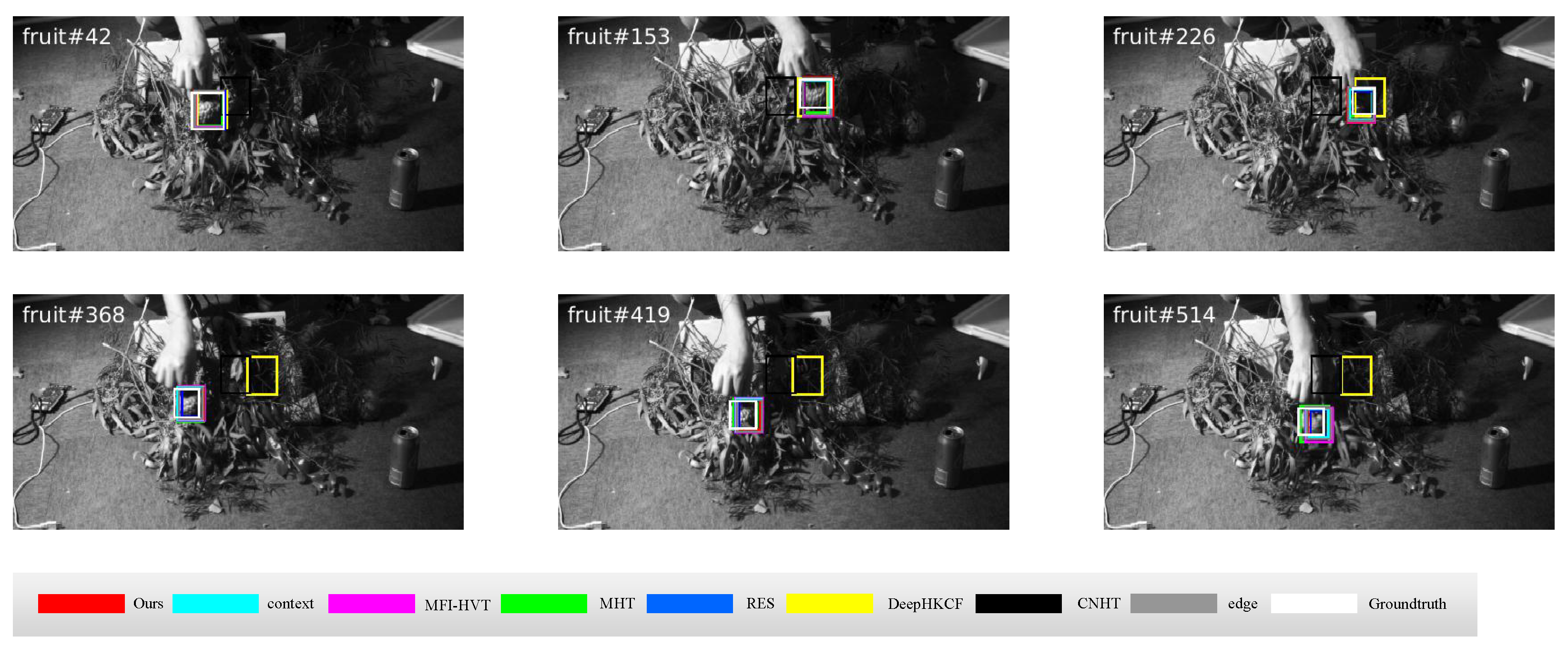
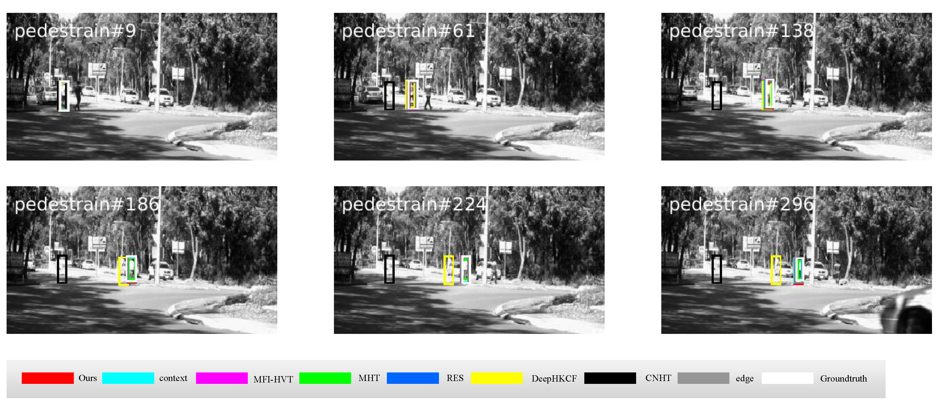
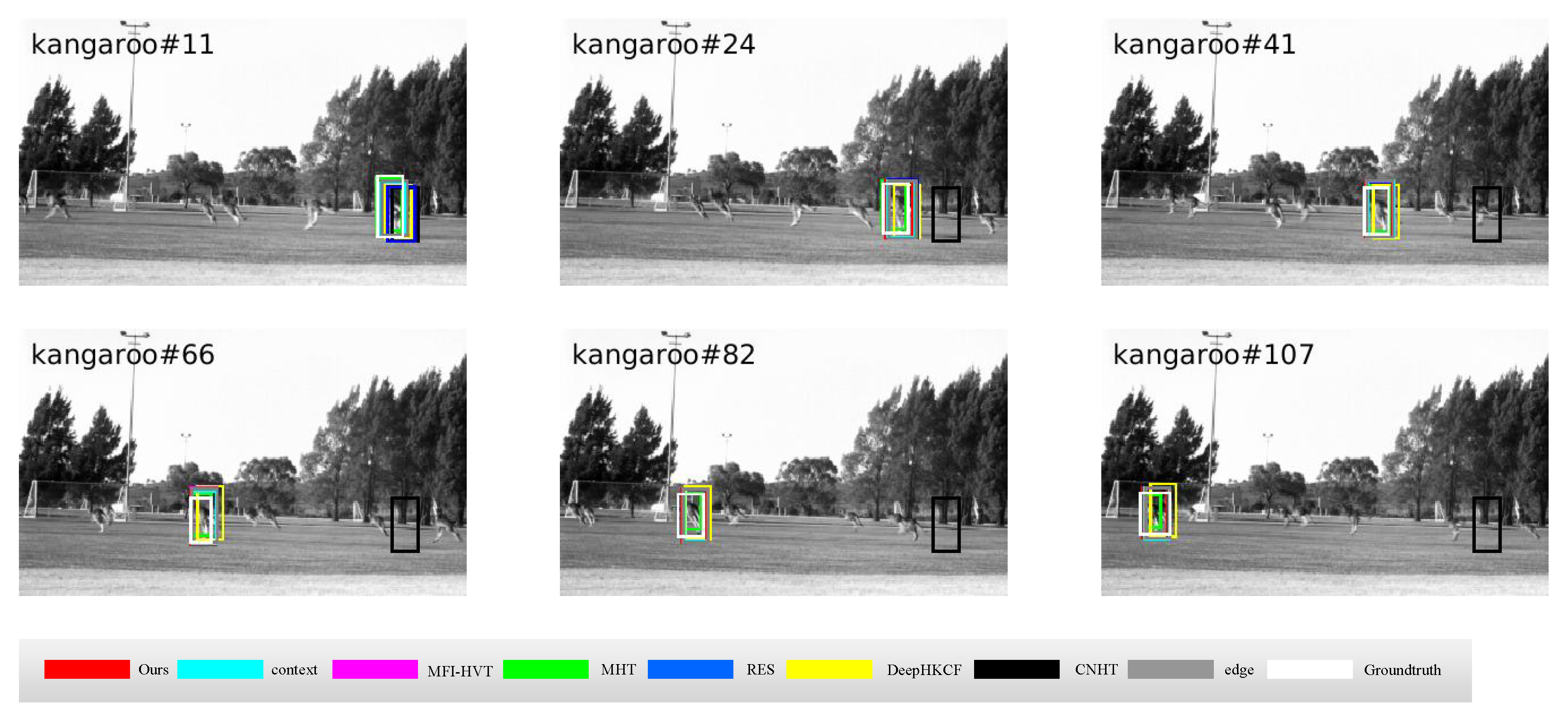
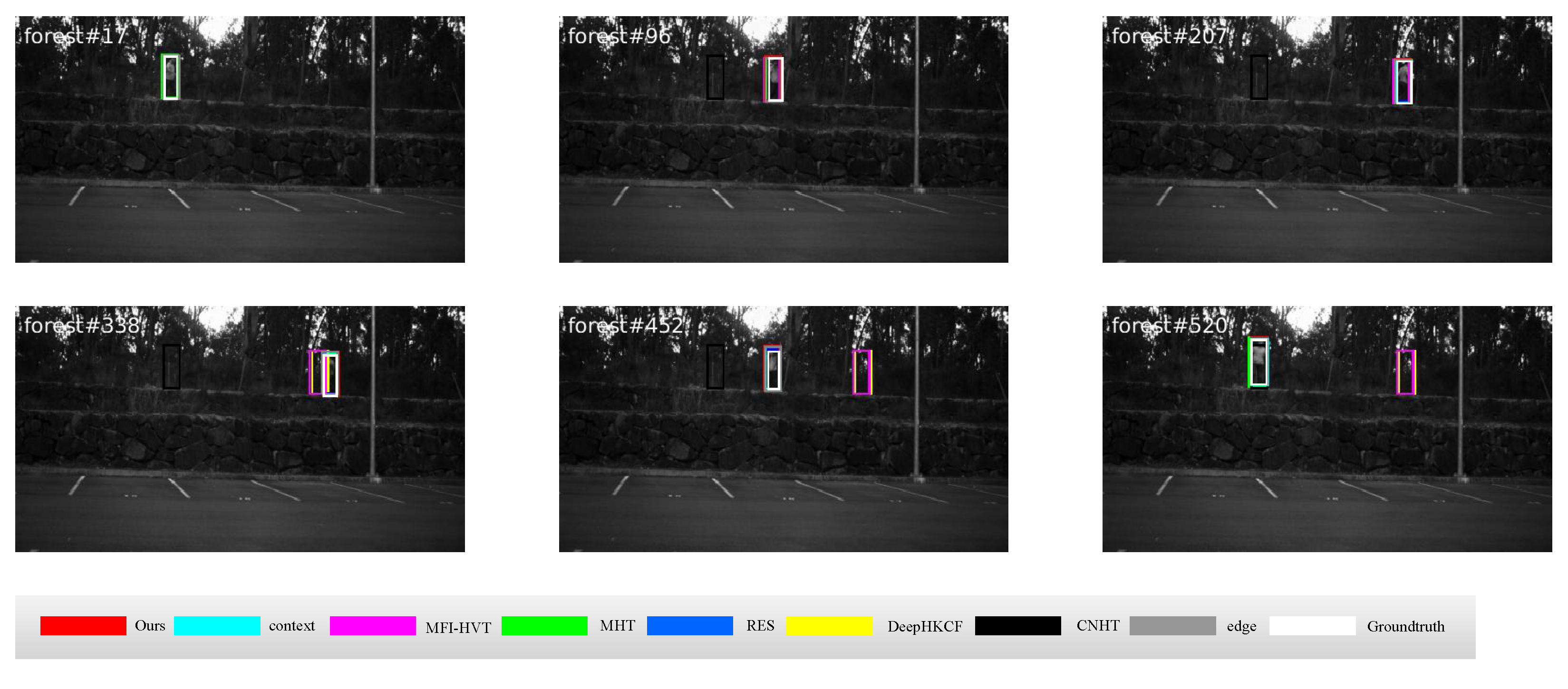
4.2. Qualitative Comparison

In this experiment, we compare the performance of our algorithm and other hyperspectral target trackers, including MFI-HVT [18], MHT [17], DeepHKCF [15], CNHT [16], context, edge and RES. In MFI-HVT, multiple features are used instead of a single feature. The MHT approach extracts the material information of the target, by using SSHMG, to distinguish the targets and backgrounds of similar color. In the DeepHKCF technique, features are extracted by using a trained deep convolutional network, and ROI mapping is employed to improve the robustness and computational efficiency. In CNHT, features are extracted by using a double-layer convolutional network to facilitate discriminative information. For the RES approach, the features extracted from the dimensionally-reduced image via Resnet50 are used to track the target. To verify the effectiveness of the improved context filter and 3D edge features, two compared algorithms named context and edge are used. Different from our algorithm, the context algorithm uses CACF, and the edge algorithm only uses 3D edge features in the feature-extraction module.

The results of the proposed algorithm and seven other algorithms discussed in this paper, over the six test sequences, are summarized in Figure 11, Figure 12, Figure 13, Figure 14, Figure 15 and Figure 16.

In Figure 11, the background is filled with similar coins, making it difficult to track the target accurately, and the coins are pinched and moved by the fingers throughout the sequence causing the target to be partially obscured. DeepHKCF does not adapt well to the background clutter during tracking, making it drift throughout the tracking process. The edge and the context tracked robustly throughout the coin sequence, showing good performance to the challenge of background clutter.

In Figure 12, the fruit moves above the leaves, causing a change in size making tracking difficult. The MHT, MFI-HVT, and the proposed algorithm take advantage of the spectral characteristics of the target and perform well in this sequence. However, CNHT substitutes too much background clutter in the tracking process leading to tracking failure at frame 153.

In Figure 13, the pedestrian walks from the shadows into the sunlight, causing the pedestrian to become smaller and smaller. Methods such as MHT and DeepHKCF do not have a target frame estimation module, resulting in the drifting of the target frame after frame 224.

In Figure 14, there is some background interference due to the rapid jumping of the kangaroo and the similarity of the tracked kangaroo with other kangaroos. Most of the trackers perform well on this sequence as most of them use target features.

In Figure 15, the drive moves over a cluttered background, causing the drive to deform due to directional shifts. During the tracking process, the target changes frequently, causing the fact that the target boxes of all trackers do not adapt well to the changes of the target. However, at frame 599, our tracker overlaps perfectly with the ground truth.

In Figure 16, the target walks in front of the trees and a portion of the forest causes occlusion of the target. Hence, MFI-HVT and DeepHKCF, which use depth features, lose the target from frame 338 onward. However, our tracker is able to accurately locate the target and adapt to the changes in the target.

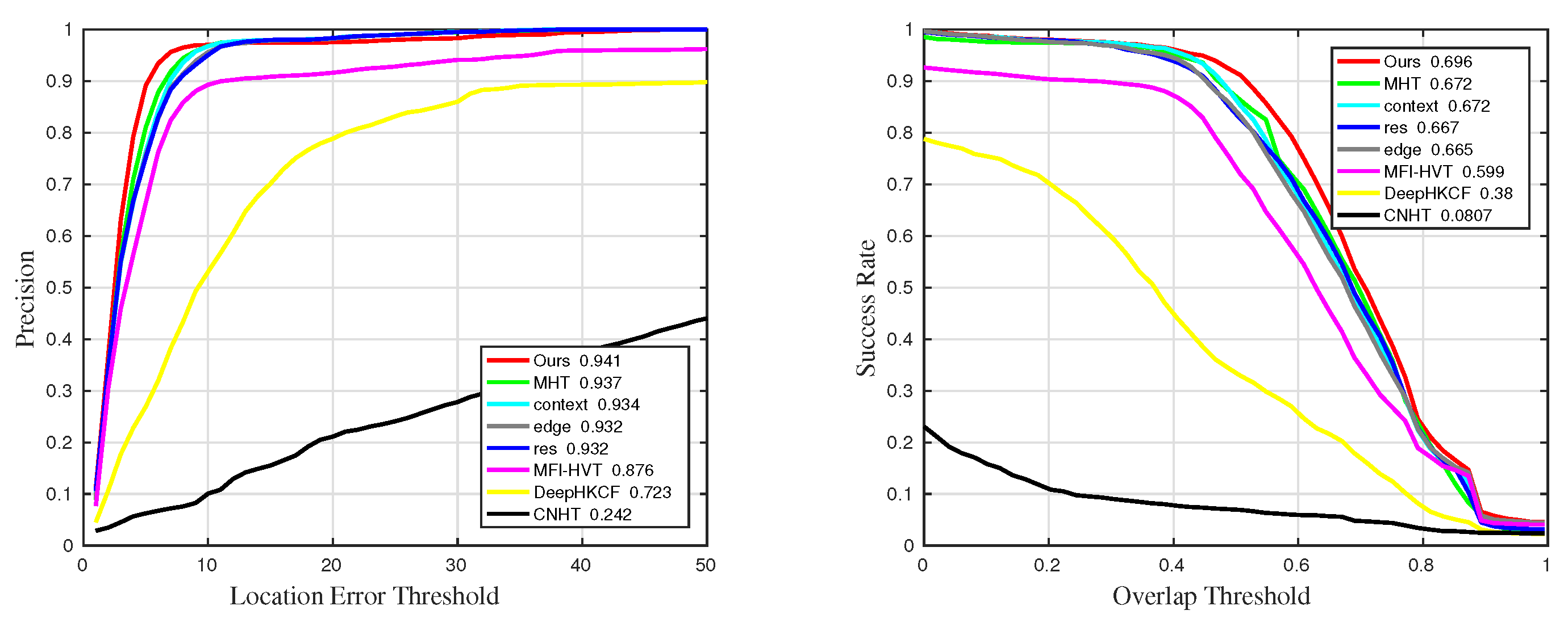
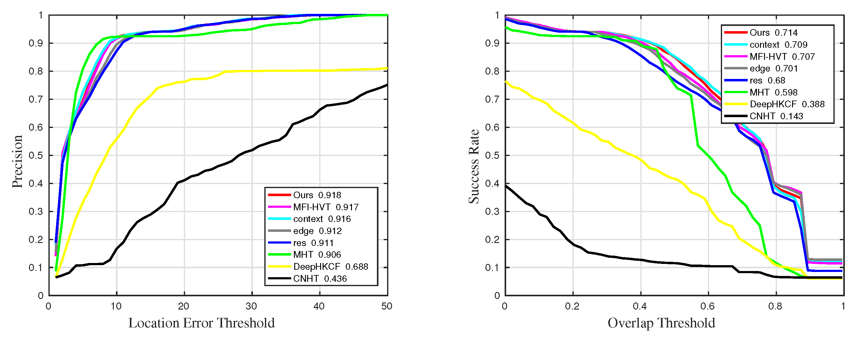
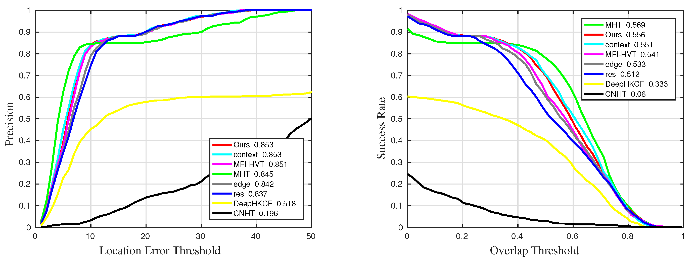
4.3. Quantitative Comparison

In this section, we compare the precision and success rate of the proposed algorithm with seven other algorithms. The precision is defined as the deviation between the centre positions of the tracking and ground truth target boxes as being not higher than a certain threshold. Similarly, the success rate is defined as the overlap between the tracking and the ground truth target boxes as being not lower than a certain threshold.

Table 2. The precision of each tracker, with a suffix indicating the challenge faced, and the top two results are highlighted in red and green respectively. The result has three significant decimal places.

Sequences	Precision	Precision_BC	Precision_OCC	Precision_SV	Precision_OPR
Ours	0.941	0.918	0.853	0.934	0.946
MHT	0.937	0.906	0.845	0.932	0.958
RES	0.932	0.911	0.837	0.93	0.947
context	0.934	0.916	0.853	0.933	0.943
edge	0.932	0.912	0.842	0.931	0.945
MFI-HVT	0.876	0.917	0.851	0.933	0.775
DeepHKCF	0.723	0.688	0.518	0.713	0.683
CNHT	0.242	0.436	0.196	0.347	0.138

and

Table 3. The success rate of each tracker, with a suffix indicating the challenge faced, and the top two results are highlighted in red and green respectively. The result has three significant decimal places.

Sequences	Success	Success_BC	Success_OCC	Success_SV	Success_OPR
Ours	0.696	0.714	0.556	0.712	0.712
MHT	0.672	0.598	0.569	0.633	0.755
RES	0.667	0.68	0.512	0.686	0.695
context	0.672	0.709	0.551	0.708	0.674
edge	0.665	0.701	0.533	0.698	0.675
MFI-HVT	0.599	0.707	0.541	0.698	0.474
DeepHKCF	0.38	0.388	0.333	0.355	0.417
CNHT	0.0807	0.143	0.06	0.106	0.0551

show the precision and success rate values for the eight algorithms. It can be observed that our algorithm has significantly improved the tracking performance. Figure 17 shows the precision and success rate curves of the algorithm on all sequences, where the higher area covered by the curve represents a higher value. Figure 18, Figure 19, Figure 20 and Figure 21 present the experimental findings related to BC, OCC, SV, and OPR, respectively.

As shown in Table 2 and Table 3, the proposed algorithm almost achieves the top two performances in terms of the various indicators. On a whole, it achieves a precision of 0.941 and a success rate of 0.696, an improvement of 0.4% and 2.4%, respectively, compared with MHT. It may be noted that MHT is the current state of the art. The edge algorithm does not show strong robustness in the whole test due to the use of a single feature. Due to the usage of DECF and ICF, our algorithm yields a better result than the other algorithms against the BC challenge. The performances of the proposed algorithm are summarized in Figure 18 and the tables. Specifically, our algorithm achieves 91.8% precision and 71.4% success rate against the BC challenge, which are significant improvements in comparison with MHT and context algorithm. MFI-HVT gets the second highest score of 91.7% precision because of the use of multifeatures. The context algorithm achieved the second highest score with a 70.9% success rate. As for the context algorithm, the success rate is 0.5% lower than ours, and the precision is 0.2% lower than ours. This is because the filter of the context algorithm is not improved. Compared with RES algorithm, the success rate of our algorithm is improved by 3.4%, and the precision is improved by 0.7%. Moreover, compared with the edge algorithm, the success rate of our algorithm is improved by 1.3%, and the precision is improved by 0.6%. These two sets of experiments show that our algorithm with DECF is more efficient than the algorithm using one feature alone. MFI-HVT shows a poor performance of 77.5% precision and 47.4% success rate in the OPR challenge. The overall performance indicates that the MFI-HVT algorithm does not have strong robustness. Additionally, as is evident from Figure 19, when the target is obscured, our algorithm has a success rate 1.3% lower than MHT but ranks first in terms of precision. Although the consideration of material features in MHT facilitate adaptive target recognition, it fails for accurate scale estimation. As shown in Figure 20, our algorithm outperforms other algorithms owing to the adaptive scale estimation even when the target is affected by deformation. As shown in Figure 21, when the target is affected by OPR, the accuracy is only 1.2% lower and the success rate is only 4.3% lower as compared to MHT.

5. Conclusions

This paper proposes an algorithm based on DECF and ICF for HSV-based target tracking. The proposed DECF is composed of both the 3D edge features and deep features of the HSIs. DECF can extract the representation of the targets which have similar color as the background. The use of ICF ensures that the tracker remains robust even under BC challenges. Extensive experiments have been conducted by using different HSVs sequences to demonstrate the superior performance of the proposed algorithm. In future work, the HSIs’ dimensionality reduction process will be further investigated to utilise the spectral information to extract the target features.

References

1. Zhang, Z.P.; Liu, Y.H.; Wang, X.; Li, B. Learn to Match: Automatic Matching Network Design for Visual Tracking. In Proceedings of the International Conference on Computer Vision, Montreal, QC, Canada, 11–17 October 2021. [Google Scholar]
2. Wang, X.; Shu, X.; Zhang, Z.; Jiang, B.; Wang, Y.; Tian, Y.; Wu, F. Towards More Flexible and Accurate Object Tracking with Natural Language: Algorithms and Benchmark. In Proceedings of the Conference on Computer Vision and Pattern Recognition, Nashville, TN, USA, 19–25 June 2021. [Google Scholar]
3. Zhao, D.; Gu, L.; Qian, K.; Zhou, H.; Cheng, K. Target tracking from infrared imagery via an improved appearance model. Infrared Phys. Technol. 2019, 104, 103–116. [Google Scholar] [CrossRef]
4. Bhat, G.; Danelljan, M.; Gool, L.V.; Timofte, R. Learning Discriminative Model Prediction for Tracking. In Proceedings of the International Conference on Computer Vision, Chongqing, China, 23–28 August 2020. [Google Scholar]
5. Marques, J.S.; Jorge, P.M.; Abrantes, A.J.; Lemos, J.M. Tracking Groups of Pedestrians in Video Sequences. In Proceedings of the Computer Vision and Pattern Recognition Workshop, Madison, MI, USA, 16–22 June 2003. [Google Scholar]
6. Li, D.; Zhang, Z.; Chen, X.; Huang, K. A Richly Annotated Pedestrian Dataset for Person Retrieval in Real Surveillance Scenarios. IEEE Trans. Image Process. 2019, 28, 1575–1590. [Google Scholar] [CrossRef] [PubMed]
7. Xiang, Y.; Alahi, A.; Savarese, S. Learning to Track: Online Multi-object Tracking by Decision Making. In Proceedings of the International Conference on Computer Vision, Santiago, Chile, 11–18 December 2015. [Google Scholar]
8. Ravankar, A.; Ravankar, A.A.; Kobayashi, Y.; Hoshino, Y. Path Smoothing Techniques in Robot Navigation: State-of-the-Art, Current and Future Challenges. Sensors 2018, 18, 3170. [Google Scholar] [CrossRef] [PubMed] [Green Version]
9. Ojha, S.; Sakhare, S. Image processing techniques for object tracking in video surveillance—A survey. In Proceedings of the International Conference on Pervasive Computing, St. Louis, MO, USA, 23–27 March 2015. [Google Scholar]
10. Dorfler, F.; Jovanovic, M.R.; Chertkov, M.; Bullo, F. Sparsity-Promoting Optimal Wide-Area Control of Power Networks. IEEE Trans. Power Syst. 2013, 29, 2281–2291. [Google Scholar] [CrossRef] [Green Version]
11. Hong, D.; Han, Z.; Yao, J.; Gao, L.; Zhang, B.; Plaza, A.; Chanussot, J. SpectralFormer: Rethinking Hyperspectral Image Classification with Transformers. IEEE Trans. Geosci. Remote Sens. 2021, 60, 1–15. [Google Scholar] [CrossRef]
12. Uzair, M.; Mahmood, A.; Mian, A. Hyperspectral Face Recognition With Spatiospectral Information Fusion and PLS Regression. IEEE Trans. Image Process. 2015, 24, 1127–1137. [Google Scholar] [CrossRef]
13. Prasad, S.; Bruce, L.M. Decision fusion with confidence-based weight assignment for hyperspectral target recognition. IEEE Trans. Geosci. Remote Sens. 2008, 46, 1448–1456. [Google Scholar] [CrossRef]
14. Naoto, Y.; Jonathan, C.; Karl, S. Potential of Resolution-Enhanced Hyperspectral Data for Mineral Mapping Using Simulated EnMAP and Sentinel-2 Images. Remote Sens. 2016, 8, 172. [Google Scholar] [CrossRef] [Green Version]
15. Uzkent, B.; Rangnekar, A.; Hoffman, M.J. Tracking in Aerial Hyperspectral Videos Using Deep Kernelized Correlation Filters. IEEE Trans. Geosci. Remote Sens. 2018, 57, 449–461. [Google Scholar] [CrossRef] [Green Version]
16. Qian, K.; Zhou, J.; Xiong, F.; Zhou, H.; Du, J. Object Tracking in Hyperspectral Videos with Convolutional Features and Kernelized Correlation Filter. Int. Conf. Smart Multimed. 2018, 11010, 308–319. [Google Scholar]
17. Xiong, F.; Zhou, J.; Qian, Y. Material Based Object Tracking in Hyperspectral Videos. IEEE Trans. Image Process. 2020, 29, 3719–3733. [Google Scholar] [CrossRef] [PubMed]
18. Zhang, Z.; Qian, K.; Du, J.; Zhou, H. Multi-Features Integration Based Hyperspectral Videos Tracker. In Proceedings of the IEEE Workshop on Hyperspectral Image and Signal Processing: Evolution in Remote Sensing, Amsterdam, The Netherlands, 24–26 March 2021. [Google Scholar]
19. Martinez, A.M.; Kak, A.C. PCA versus LDA. IEEE Trans. Pattern Anal. Mach. Intell. 2002, 23, 228–233. [Google Scholar] [CrossRef] [Green Version]
20. Jian, Y.; David, Z.; Frangi, A.F.; Jing, Y. Two-dimensional PCA: A new approach to appearance-based face representation and recognition. IEEE Trans. Pattern Anal. Mach. Intell. 2004, 26, 131–137. [Google Scholar] [CrossRef] [PubMed] [Green Version]
21. He, K.; Zhang, X.; Ren, S.; Sun, J. Deep Residual Learning for Image Recognition. In Proceedings of the IEEE Conference on Computer Vision and Pattern Recognition, Las Vegas, NV, USA, 27–30 June 2016. [Google Scholar]
22. Clausi, D.A.; Jernigan, M.E. Designing Gabor filters for optimal texture separability. Pattern Recognit. 2000, 33, 1835–1849. [Google Scholar] [CrossRef]
23. Guo, Z.; Zhang, L.; Zhang, D. A completed modeling of local binary pattern operator for texture classification. IEEE Trans. Image Process. 2010, 19, 1657–1663. [Google Scholar]
24. Benediktsson, J.A.; Palmason, J.A.; Sveinsson, J.R. Classification of hyperspectral data from urban areas based on extended morphological profiles. IEEE Trans. Geosci. Remote Sens. 2005, 43, 480–491. [Google Scholar] [CrossRef]
25. Zhu, J.; Hu, J.; Jia, S.; Jia, X.; Li, Q. Multiple 3-D feature fusion framework for hyperspectral image classification. IEEE Trans. Geosci. Remote Sens. 2018, 56, 1873–1886. [Google Scholar] [CrossRef]
26. Li, W.; Chen, C.; Su, H.; Du, Q. Local binary patterns and extreme learning machine for hyperspectral imagery classification. IEEE Trans. Geosci. Remote Sens. 2015, 53, 3681–3693. [Google Scholar] [CrossRef]
27. Tu, B.; Kuang, W.; Zhao, G.; He, D.; Liao, Z.; Ma, W. Hyperspectral image classification by combining local binary pattern and joint sparse representation. Int. J. Remote Sens. 2019, 40, 9484–9500. [Google Scholar] [CrossRef]
28. LeCun, Y.; Bengio, Y.; Hinton, G. Deep learning. Nature 2015, 521, 436–444. [Google Scholar] [CrossRef]
29. Kamilaris, A.; Prenafeta-Boldú, F.X. Deep learning in agriculture: A survey. Comput. Electron. Agric. 2018, 147, 70–90. [Google Scholar] [CrossRef] [Green Version]
30. Chen, Y.; Zhao, X.; Jia, X. Spectral–spatial classification of hyperspectral data based on deep belief network. IEEE J. Sel. Top. Appl. Earth Obs. Remote Sens. 2015, 8, 2381–2392. [Google Scholar] [CrossRef]
31. He, M.; Li, B.; Chen, H. Multi-scale 3D deep convolutional neural network for hyperspectral image classification. In Proceedings of the 2017 IEEE International Conference on Image Processing (ICIP), Beijing, China, 17–20 September 2017; pp. 3904–3908. [Google Scholar]
32. Bolme, D.S.; Beveridge, J.R.; Draper, B.A.; Lui, Y.M. Visual object tracking using adaptive correlation filters. In Proceedings of the 2010 IEEE Computer Society Conference on Computer Vision and Pattern Recognition, San Francisco, CA, USA, 13–18 June 2010. [Google Scholar]
33. Henriques, J.F.; Rui, C.; Martins, P.; Batista, J. Exploiting the Circulant Structure of Tracking-by-Detection with Kernels. Eur. Conf. Comput. Vis. 2012, 7575, 702–715. [Google Scholar]
34. Tappen, M.F.; Freeman, W.T.; Adelson, E.H. Recovering Intrinsic Images from a Single Image. IEEE Trans. Pattern Anal. Mach. Intell. 2005, 27, 1459–1472. [Google Scholar] [CrossRef] [PubMed]
35. Henriques, J.F.; Caseiro, R.; Martins, P.; Batista, J. High-Speed Tracking with Kernelized Correlation Filters. IEEE Trans. Pattern Anal. Mach. Intell. 2015, 37, 583–596. [Google Scholar] [CrossRef] [Green Version]
36. Kiani Galoogahi, H.; Fagg, A.; Lucey, S. Learning background-aware correlation filters for visual tracking. In Proceedings of the IEEE International Conference on Computer Vision, Venice, Italy, 22–29 October 2017; pp. 1135–1143. [Google Scholar]
37. Danelljan, M.; Hager, G.; Shahbaz Khan, F.; Felsberg, M. Learning spatially regularized correlation filters for visual tracking. In Proceedings of the IEEE International Conference on Computer Vision, Santiago, Chile, 11–18 December 2015; pp. 4310–4318. [Google Scholar]
38. Mueller, M.; Smith, N.; Ghanem, B. Context-Aware Correlation Filter Tracking. In Proceedings of the IEEE Conference on Computer Vision and Pattern Recognition, Honolulu, HI, USA, 21–26 July 2017; pp. 1396–1404. [Google Scholar]
39. Li, Y.; Zhu, J. A scale adaptive kernel correlation filter tracker with feature integration. In Proceedings of the European Conference on Computer Vision, Zurich, Switzerland, 6–12 September 2014; pp. 254–265. [Google Scholar]
40. Martin, D.L.; Häger, G.; Fahad, S.; Michael, F. Accurate Scale Estimation for Robust Visual Tracking. In Proceedings of the British Machine Vision Conference, Nottingham, UK, 1–5 September 2014. [Google Scholar]
41. Danelljan, M.; Häger, G.; Khan, F.S.; Felsberg, M. Discriminative scale space tracking. IEEE Trans. Pattern Anal. Mach. Intell. 2016, 39, 1561–1575. [Google Scholar] [CrossRef] [PubMed] [Green Version]
42. Bertinetto, L.; Valmadre, J.; Henriques, J.F.; Vedaldi, A.; Torr, P. Fully-Convolutional Siamese Networks for Object Tracking. In Proceedings of the European Conference on Computer Vision, Amsterdam, The Netherlands, 11–14 October 2016; pp. 850–865. [Google Scholar]
43. Li, B.; Yan, J.; Wei, W.; Zheng, Z.; Hu, X. High Performance Visual Tracking with Siamese Region Proposal Network. In Proceedings of the IEEE Conference on Computer Vision and Pattern Recognition, Salt Lake City, UT, USA, 18–22 June 2018. [Google Scholar]
44. Li, B.; Wu, W.; Wang, Q.; Zhang, F.; Xing, J.; Yan, J. SiamRPN++: Evolution of Siamese Visual Tracking With Very Deep Networks. In Proceedings of the IEEE Conference on Computer Vision and Pattern Recognition, Seattle, WA, USA, 13–19 June 2020. [Google Scholar]
45. Skurikhin, A.N.; Garrity, S.R.; McDowell, N.G. Automated tree crown detection and size estimation usingmulti-scale analysis of high-resolution satellite imagery. Remote Sens. Lett. 2013, 4, 465–474. [Google Scholar] [CrossRef]
46. Witkin, A.P. Scale-space filtering: A new approach to multi-scale description. In Proceedings of the IEEE International Conference on Acoustics, Speech, and Signal Processing, San Diego, CA, USA, 19–21 March 1984. [Google Scholar]
47. Lowe, D. Distinctive image features from scale-invariant key points. Int. J. Comput. Vis. 2003, 20, 91–110. [Google Scholar]
48. Cheng, X.; Chen, Y.; Tao, Y.; Wang, C.; Kim, M.; Lefcourt, A. A novel integrated PCA and FLD method on hyperspectral image feature extraction for cucumber chilling damage inspection. Trans. ASAE 2004, 47, 1313. [Google Scholar] [CrossRef]
49. Gu, J.; Wang, Z.; Kuen, J.; Ma, L.; Gang, W. Recent Advances in Convolutional Neural Networks. Pattern Recognit. 2015, 77, 354–377. [Google Scholar] [CrossRef] [Green Version]
50. Dalal, N.; Triggs, B. Histograms of oriented gradients for human detection. In Proceedings of the 2005 IEEE Computer Society Conference on Computer Vision and Pattern Recognition, San Diego, CA, USA, 20–25 June 2005; pp. 886–893. [Google Scholar]
51. Martins, V.S.; Kaleita, A.L.; Gelder, B.K.; da Silveira, H.L.; Abe, C.A. Exploring multiscale object-based convolutional neural network (multi-OCNN) for remote sensing image classification at high spatial resolution. ISPRS J. Photogramm. Remote Sens. 2020, 168, 56–73. [Google Scholar] [CrossRef]
52. Vincent, O.R.; Folorunso, O. A descriptive algorithm for sobel image edge detection. In Proceedings of the Informing Science & IT Education Conference (InSITE), Macon, GA, USA, 12–15 June 2009; Volume 40, pp. 97–107. [Google Scholar]
53. Kanopoulos, N.; Vasanthavada, N.; Baker, R.L. Design of an image edge detection filter using the Sobel operator. IEEE J. Solid-State Circuits 1988, 23, 358–367. [Google Scholar] [CrossRef]
Figure 1. The framework of our tracker.
Remotesensing 14 06219 g001
Figure 2. The results after PCA dimensionality reduction.
Remotesensing 14 06219 g002
Figure 3. The first 128 channels of deep features.
Remotesensing 14 06219 g003
Figure 4. (a) the distribution of the pixel in the center of I x and surrounding pixels; (b) the distribution of the pixel in the center of I y and surrounding pixels; (c) the distribution of the pixel in the center of I z and surrounding pixels.
Remotesensing 14 06219 g004
Figure 5. Edge features in 16 bands.
Remotesensing 14 06219 g005
Figure 6. Fusion process of DECF.
Remotesensing 14 06219 g006
Figure 7. Fused DECF.
Remotesensing 14 06219 g007
Figure 8. Contextual sampling area diagram.
Remotesensing 14 06219 g008
Figure 9. Response map after background suppression.
Remotesensing 14 06219 g009
Figure 10. Six RGB experiments.
Remotesensing 14 06219 g010
Figure 11. Qualitative outcomes for the coin sequence.
Remotesensing 14 06219 g011
Figure 12. Qualitative outcomes for the fruit sequence.
Remotesensing 14 06219 g012
Figure 13. Qualitative outcomes for the pedestrian sequence.
Remotesensing 14 06219 g013
Figure 14. Qualitative outcomes for the kangaroo sequence.
Remotesensing 14 06219 g014
Figure 15. Qualitative outcomes for the drive sequence.
Remotesensing 14 06219 g015
Figure 16. Qualitative outcomes for the forest sequence.
Remotesensing 14 06219 g016
Figure 17. Precision and success rate under the overall sequence.
Remotesensing 14 06219 g017
Figure 18. Precision and success rate under BC challenge.
Remotesensing 14 06219 g018
Figure 19. Precision and success rate under OCC challenge.
Remotesensing 14 06219 g019
Figure 20. Precision and success rate under SV challenge.
Remotesensing 14 06219 g020
Figure 21. Precision and success rate under OPR challenge.
Remotesensing 14 06219 g021