Article

Satellite and sUAS Multispectral Remote Sensing Analysis of Vegetation Response to Beaver Mimicry Restoration on Blacktail Creek, Southwest Montana

1
Department of Environmental Engineering, Montana Technological University, 1300 W. Park Street, Butte, MT 59701, USA
2
Montana Bureau of Mines and Geology, Montana Technological University, 1300 W. Park Street, Butte, MT 59701, USA
3
Department of Geological Engineering, Montana Technological University, 1300 W. Park Street, Butte, MT 59701, USA
*
Author to whom correspondence should be addressed.
These authors contributed equally to this work.
Remote Sens. 2022, 14(24), 6199; https://doi.org/10.3390/rs14246199
Submission received: 2 October 2022 / Revised: 25 November 2022 / Accepted: 2 December 2022 / Published: 7 December 2022
(This article belongs to the Section Environmental Remote Sensing)

Abstract

:
Beaver dam analogs (BDAs) are being installed on streams where restoration goals include reconnecting the stream to its floodplain, increasing water storage in the stream corridor, and improving the extent and vigor of riparian vegetation. This study evaluated the effects on vegetation vigor of a BDA treatment on Blacktail Creek in southwest Montana, USA, using data from Sentinel-2 satellites and a small unmanned aerial system (sUAS; a.k.a. drone). The goal of this research was to determine if BDA installation increased the health of riparian vegetation. Sentinel-2 remote sensing data from 2016 to 2021 were used to compare the pre- and post-treatment periods, and to evaluate effects in the treated area relative to control areas. Enhanced Vegetation Index (EVI) values were calculated to quantify vegetation response from the addition of BDAs. These data suggest that installing BDAs at this site has not led to an apparent increase in late-summer vegetation vigor relative to the controls. One potential explanation for these results is that the vegetation was not water limited prior to treatment in this study reach. This is an important consideration for water resource managers prior to installation of BDAs if the main restoration goal is the improvement of riparian vegetation health. Two high spatial resolution sUAS multispectral datasets were collected to evaluate the bias introduced by using the relatively course resolution (10 m) satellite imagery to assess these changes. High-resolution sUAS data allow fine-scale differences in vegetation and inundated area to be distinguished; however, historical sUAS datasets are rarely available. Satellite-based remote sensing has much lower resolution; however, Sentinel-2 satellite data have been available for the entire earth since 2016. This study demonstrates that the combination of sUAS and satellite based remote sensing data provides a method to compare high-resolution datasets for spatial analysis while gaining insight into relatively low-resolution historical data for temporal analysis.

1. Introduction

Climate change related shifts in the timing of runoff and peak streamflow have been observed in mountainous areas, and further shifts are predicted; for example, see [1,2]. For instance, in western Montana, US, it is anticipated that winter precipitation will increase, but there will be less snowpack due to a shift in the form of precipitation from snow to rain [3]. Restoration projects such as beaver dam analogs (BDAs) have been used to aid in the establishment and maintenance of riparian ecosystems during drought periods [4,5], and they are thought to aid in maintaining late-summer streamflow due to increased water storage within the stream corridor [4]. Riparian ecosystems only occupy a small portion of most landscapes, yet have a disproportionate influence on wildlife, vegetation, and water resources [6]. BDAs are simple rock and/or wood structures placed in the bed of an incised stream [4,7,8]. BDAs are thought to help maintain dry-season streamflow by increasing groundwater and surface-water storage [4,9,10], which is particularly important where snowpack water storage is declining. The use of BDAs in restoration is becoming increasingly popular due to their simplicity and perceived benefits [4,7]. The higher stream stages created by BDAs also cause increased groundwater elevations near the structures [4,11,12,13,14], and decreased depth to groundwater likely causes evapotranspiration (ET) to increase [3,6,15]. It has been suggested that the increased ET may more than offset increases in streamflow due to higher groundwater storage [15].
Satellite-based remote sensing analysis has been used since the early 1970s to understand physical states and processes at the earth’s surface [16]. The use of satellite-based remote sensing to evaluate the effectiveness of stream restoration techniques is increasing [17]. Many studies have used satellite-based remote sensing data to monitor changes in riparian vegetation [18,19,20,21]. The commercial usage of small unmanned aerial systems (sUAS) became widely available in the United States in 2006, after the US Federal Aviation Administration issued the first commercial drone permit [22]. Since then, there have been unprecedented advances in sUAS technologies. These advances are lowering the cost and accessibility of high-resolution earth observation data collection. The use of sUAS can leverage knowledge of space-based remote sensing to increase the spatial, spectral, and temporal resolution at which we can investigate earth processes. The increasing usage of multispectral data allows for greater opportunities to monitor riparian systems across a variety of watershed sizes and flow conditions [3]. Multispectral sUASs can map photosynthetic vegetation cover at high spatial resolution, and this has led to their increased use in hydrological and ecological research [23]. For example, sUAS imagery has been used to observe increases in riparian chlorophyll content and stream surface area immediately upstream of BDAs [3], which was effective for streams with approximate widths of 1.5 m or larger.
The changes in vegetation vigor due to BDA installations have not been evaluated in many areas, and studies have generally not been conducted at relatively wet sites in high elevation headwater systems. Similarly, the related changes in actual evapotranspiration (ETa) have not been explicitly explored. It has also been shown that using remote sensing techniques that have a pixel size larger than the stream can produce biased results [3]. To address these needs, we used the Enhanced Vegetation Index (EVI) from Sentinel-2 satellites (2016–2021) to evaluate the changes in vegetation vigor for a mountain headwaters site where BDAs were installed in October 2016. We also used a sUAS to collect multispectral imagery (8 cm resolution) to calculate EVI and ETa in May and July 2020. The sUAS imagery covered the treatment reach and one control reach and was compared to Sentinel-2 (10 m resolution) imagery to evaluate the effects of using slightly different sensors with varying spatial resolutions.

2. Methods

2.1. Study Area

The study reaches (one treatment and three control reaches) are located near Butte, Montana, along Lime Kiln Road (Figure 1). The area includes a segment of upper Blacktail Creek which meanders through a small valley. Vegetation in the floodplain consists of willow, grasses, and shrubs, with some scattered conifers. The adjacent hillslopes consist of coniferous forest. This site is at an elevation of approximately 1980 m above mean sea level (AMSL), and the watershed area is approximately 235 km2 [24]. Ten BDA structures were installed along the treatment reach in October of 2016. There is an abandoned, breeched beaver dam that extends east and west across the treatment site (Figure 1). Three control reaches were selected (Figure 1) to ensure that differences between the treatment and the controls were due to the treatment rather than site-specific effects at a single control.
This study combined the use of satellite imagery with sUAS imagery to analyze vegetation changes. Historical satellite imagery was used to conduct pre- and post-restoration comparisons at the treatment site, and to compare the treated and control reaches. sUAS multispectral data were used to provide high resolution imagery for comparison of the treated and control reaches during the spring and summer of 2020; however, no pre-treatment data were available (a typical situation for a restoration project). The enhanced vegetation index (EVI, Table 1) was used to evaluate plant productivity along these reaches. EVI is essentially an estimate of chlorophyll content of the imaged vegetation [25]. The EVI values were used to estimate ETa [26].
The BDAs were constructed using wooden posts driven into the streambed and woven with branches, mud, and grass (Figure 2). The structures create upstream pools that collect sediment and organic matter, slow water movement, increase channel width and stream stage, and allow for greater connectivity to the floodplain during high flows [3]. In the treatment reach, there are seven BDA structures on the main stem of the stream and three structures along a tributary feeding into Blacktail Creek. Control reach 1 was the primary control reach and is approximately 520 m upstream from the treatment reach. Control reach 2 was located approximately 450 m east of the treatment reach on a tributary. Control reach 3 was located approximately 490 m downstream of the treatment reach on the main stem. For ease of analysis using multispectral remote sensing, the four study reaches were created using the same size (63 × 139 m) and orientation (Figure 1). The plan view area of all three control reaches and treatment reach is 8366 m2. Additionally, from visual observations, it was noted that the study reaches have similar vegetation, hydrology, topography, and floodplain area.
The study site is approximately 5.8 km from the Basin Creek SNOTEL site [27] which is at an elevation of 2190 m AMSL. For the years 1981–2020, the average precipitation was 625 mm and the maximum average snow water equivalent of 229 mm occurred in early May. In most cases in Montana, there is more precipitation at higher elevations. The average temperature from 1991 to 2019 was 3 °C, and July was the warmest month with a mean temperature of 15 °C.

2.2. Hydrologic and Hydrogeologic Monitoring

Hydrologic data (i.e., streamflows and groundwater levels) for treatment reach and control reach 1 (Figure 1) were collected during a previous study [24]. Groundwater elevation measurements were collected from May to July of 2020 to supplement previous monitoring (2016–2019; [24]. Depth to water measurements were collected manually using a Solinst e-tape (an electronic sounder) on three occasions (10 May 2020, 19 June 2020, and 19 July 2020). For each event, measurements were obtained from 12 wells in control reach 1, and 21 wells in the treatment reach (Figure 3). All wells were surveyed with a global navigation satellite system (GNSS) receiver to establish measuring point elevations. Stream stage and stream discharge were measured on the same dates as the groundwater measurements, with additional measurements on 23 August 2020. Stream discharge and stage were measured in the treatment reach (SW_UT, SW_M1T, SW_M2T, and SW_DT) and the control reach (SW_UC and SW_DC) (Figure 3). Stream discharge was measured using a Marsh McBirney Flow-Mate.

2.3. Sentinel-2 Data

The Sentinel-2 multispectral data for the summers of 2016–2021 were acquired from the Copernicus Open Access Hub [28]. Sentinel-2 has a 10 m pixel resolution for the bands required for this study (blue, red, and NIR; Table 2). Sentinel-2 has a temporal resolution of 10 days for each satellite and 5 days between the identical Sentinel A and B satellites. The USGS Earth Explorer website was used to verify the presence or absence of cloud coverage of the study reaches for each imaged day. Prior to December 2018, only Level-1C format imagery (top of atmosphere product) is available [29]. Beginning in December 2018, Level-2A format data (bottom of the atmosphere) were available for download. Level-2A products are derived from Level-1C data products and provide bottom of atmosphere reflectance. The bottom of atmosphere reflectance is essentially the reflectance directly above the vegetation surface [30]. To be consistent, for this study, Level-1C was downloaded for all time periods and then converted to Level-2A using ESA’s Sen2Cor (v2.10) processor in the SNAP program [31]. The resulting rasters were clipped to the treatment and control reaches.

2.4. sUAS Data Collection and Processing

2.4.1. sUAS Multispectral Data Collection

Multispectral imagery was collected by sUAS-based multispectral remote sensing on 5/10/20 and 7/19/20. The sUAS system used for this research consisted of a DJI Matrice 600 Pro with a MicaSense RedEdge-MX and RedEdge-MX Blue multispectral cameras. When both cameras are paired together the system is referred to as the dual camera system. The combined sensors capture ten spectral reflectance bands (Table 2 and Figure 4). Incorporating the ten bands of the dual camera system makes the band wavelengths approximately comparable to that of Sentinel-2 (Figure 4). The bands used for EVI calculations are blue, red, and near infrared (Bands 2, 4, and 5 in Table 2). Combining the red bands from the RedEdge-MX (band 3) and the RedEdge-MX Blue (band 8) provides the best overlap with Sentinel-2 red band. However, during analysis, it was noted that there is no statistical difference between red bands from the RedEdge-MX and the RedEdge-MX Blue (Appendix B). Hence, only RedEdge-MX blue, red, and near infrared (Bands 2, 4, and 5 in Table 2) bands were used in EVI calculation. The dual camera system was calibrated using a MicaSense calibration panel with known reflectance values. Before each flight campaign, the sUAS was held above the calibration panel and images were manually obtained [33].
The sUAS automated flight plan was created with the program Pix4D Capture [34] for multispectral image acquisition (Figure 5). The dual camera system captured 10 images, one for each band, every second in 12-bit RAW data format. The treatment reach and control reach 1 were flown with 75% side and front overlap at an altitude of 120 m, resulting in 8 cm pixel resolution. The sUAS flights took place near noon and were timed to match days of Sentinel-2 data collection for consistency.

2.4.2. Ground Truth for sUAS Imagery

Five ground control points (GCPs) and five check points (CPs) were used at each study reach for multispectral data georeferencing. The targets were 30 cm bucket lids, which provided clear contrast to the background vegetation. The targets were surveyed using centimeter-level accuracy Trimble Geo7X GNSS Receiver with a Trimble Zephyr 2 Antenna. All GNSS measurements were post processed in Trimble Pathfinder Office and were output in WGS84 (2011) (horizontal) and EGM96 (vertical) datum. GCPs were used during the Structure from Motion (SfM) processing and orthorectification of the multispectral data in Pix4Dmapper to increase spatial accuracy of the multispectral mosaic model [35]. The CPs were used for unbiased evaluation of the spatial accuracy of the resulting model. For each imaged reach a GCP was staked at each corner and one was staked near the center. The five CPs were staked approximately evenly throughout each reach (Appendix A). GCPs and CPs were left at the reaches between flights to ensure consistent geolocation.

2.4.3. Image Processing

Multispectral orthomosaics were produced using Pix4Dmapper version 4.3.31 as per the procedure provided by multispectral cameras manufacturer (Micasense, [36]). Multispectral data were radiometrically processed and calibrated using the RedEdge Downwelling Light Sensor (DLS) and Micasense Calibrated Reflectance Panel (CRP). Calibration photos (of the calibrated reflectance panel) taken before flights were used in the radiometric processing. The light sensor (attached to sUAS system) measures sun angles and irradiance and works autonomously to help improve reliability of data. Both the calibration photos and the light sensor help correct radiometric errors to produce accurate reflectance data.
The calibration photos and dual camera system multispectral photos were processed in Pix4Dmapper. The known reflectance values were entered for the corresponding band calibration photos in the Pix4Dmapper. The multispectral photogrammetry products were exported in the coordinate system: World Geodetic System 1984 (WGS84 (2011)) (horizontal) and EGM96 (vertical) datum. Following the initial processing, the GCPs and CPs were manually located in the photos in Pix4D. Each GCP and CP was located in each band for at least three images. Once the GCPs and CPs were located, the model was reoptimized and then the point cloud mesh, the digital surface model (DSM), orthomosaic, and index were created. The final products were reflectance map orthomosaics and GeoTIFF files for each band.

2.5. Calculating EVI

The Enhanced Vegetation Index (EVI) is an index developed to optimize vegetation reflectance in locations with high biomass. EVI corrects for some distortions in reflected light, such as Rayleigh and ozone absorption caused by particles in the air [37], and atmospheric conditions and soil background noise [38]. The GeoTIFF files from Sentinel-2, and those created in Pix4D for the sUAS data were processed in ESRI ArcMap (Version 10.7.1) or ArcGIS Pro 2.0. EVI values were calculated using the following EVI equation [25,39], Equation (1), where NIR, Red, and Blue refer to the corresponding wavelength band reflectance values (unitless). The process for calculating EVI from the Sentinel-2 data is illustrated in Appendix A (Figure A1). ArcGIS Model Builder was used to automate the task of processing the Sentinel-2 data.
E V I = 2.5 × ( N I R R e d N I R + 6 × R e d 7.5 × B l u e + 1 )

2.6. Estimating Evapotranspiration (ETa)

Nagler et al. [40] have developed an equation to estimate ETa using EVI and a local reference crop evapotranspiration estimated from meteorological data (ETo). The authors demonstrate that the algorithm developed can predict ETa values with a high R2 value of 0.73 for riparian and agricultural land uses. Since the equation’s development, a few researchers have used [20,40,41,42] to estimate ETa. EVI values from sUAS flights were used to estimate ETa following the equation published by Nagler et al. [40]. Using “Build Raster Attribute Table” tool in ArcGIS Pro, attribute table was generated with EVI values. Each pixel within the EVI raster images contained a unique EVI value, in the range from −1 to 1. Negative values represent snow or water, while positive values represent vegetation. Negative EVI values were removed since they do not represent vegetation [20]. The positive EVI values were rescaled, so they ranged from 0 to 1. The rescaled EVI values are denoted by EVI*. This rescaling is achieved by using Equation (2). We used the 99.5 and 0.5 percentiles of the EVI pixels for EVImax and EVImin, respectively. The 99.5 and 0.5 percentiles were used rather than the absolute minimum and maximum to remove the influence of extreme outliers. It should be noted that ArcGIS Pro “Build Raster Attribute Table” strictly does not create a row for each pixel; rather, it counts same EVI pixels values in one row. Therefore, slightly lower than 99.5% value was selected for upper percentile.
E V I * = 1 ( E V I m a x E V I E V I m a x E V I m i n )
The EVI* values were used to estimate ETa using Equation (3) [40]. The ETa and ETo are in mm/day. ETo values, American Society of Civil Engineers’ Penman–Monteith standardized reference evapotranspiration [43], were obtained from the Climate Engine website [37].
E T a = E T o   [ 1.73 ( 1 e 2.25 E V I * ) 0.220 ]
Equation (3) constraints ETa with a minimum value of 0 (when EVI* = 0.05) and a maximum value of 1.3 ETo (when EVI* = 1; [40]).

3. Results

3.1. Hydrologic Data

Groundwater elevation data collected in this study were compiled with data from previous years [24] to evaluate longer-term hydrological changes (2016–2020). Within each reach, groundwater elevations rise, and fall based on seasonal precipitation and runoff. Groundwater levels are high in the spring following snowmelt, and then decrease through the summer. Treatment reach water levels indicate that water levels remain elevated in the floodplain post 2016 restoration in the center of the floodplain (Figure 6; T05), but do not show an increase post restoration near the benches (Figure 6; T07).
Flow measurements collected in the control reach 1 show that the creek is slightly losing during May and June and switches to slightly gaining (July) or gaining (August). The treatment reach, however, has the opposite trend and changes from gaining (May through July) to losing in August (Table 3). These patterns were also observed during measurements collected prior to this study [24].

3.2. Meteorological Data

Annual cumulative precipitation totals for 2016, 2017, and 2020 were relatively similar (549 mm and 554 mm, 523 mm, respectively), whereas in 2018 and 2019 the values were higher (706 mm and 640 mm, respectively) (Figure 7). The summers of 2016, 2017, and 2019 had similar monthly precipitation values; however, 2018 had higher values. It should be noted that precipitation in the month of August (dry season) was higher during 2018 and 2019.

3.3. Sentinel-2 Data

Sentinel-2 derived mean EVI values for the treatment and three control reaches were analyzed to evaluate if vegetation vigor increased post-BDA restoration (Figure 8, Figure 9 and Figure 10). Figure 8 presents raw EVI values for pre- (2016) and post-treatment (2017–2021). As year-to-year EVI changes could be influenced by weather conditions, EVI data are also analyzed for differences between treatment and controls (Figure 9). To make the tends clear, mean EVI difference (Treatment–Control, dimensionless) values for the month of August (dry season, when changes in water availability would be most apparent) were presented in Figure 10. In general, before BDA restoration (2017–2021), the treatment reach had higher mean EVI values than all three controls. This relationship does not seem to have changed following the treatment.

3.4. sUAS Remote Sensing

3.4.1. Orthomosaic Generation and Accuracy

Average ground sampling distances were 8.11 cm and 8.33 cm, for 10 May 2020 and 7/19/20, respectively. The CPs used to evaluate the spatial accuracy of the model had root mean square errors ranging from 1 to 5 cm horizontally, and 6 to 19 cm vertically (Table 4). There were 715 to 740 images for the control and 820 images for the treatment (Table 5).

3.4.2. Spatial and Temporal Variation of EVI Values

To understand the spatial and temporal variation of EVI values, sUAS EVI raster datasets from 10 May 2020 and 19 July 2020 for both control 1 and treatment reach were plotted using ArcGIS. The EVI values were classified for three ranges with the break values set at 0.2, 0.6, and 1.0, resulting in classes of 0.0–0.2 (low), 0.2–0.6 (medium), and 0.6–1.0 (high) values (Figure 11). Both control 1 and the treatment reach had low EVI values on 10 May 2020. Both reaches had larger regions of high EVI (0.6–1.0) values on 19 July 2020.

3.5. Comparing Data Sets

There are a variety of differences between satellite and sUAS RedEdge-MX multispectral data. The band wavelength ranges are not identical (Table 2 and Figure 4) and the spatial resolution is different (Figure 12). To account for the difference in resolution the sUAS multispectral data were upscaled to 10-m spatial resolution in ArcMap for comparison with the Sentinel-2 data (Table 6). The scaled RedEdge-MX EVI values were attenuated, and closer to the values of the Sentinel. EVI values calculated from scaled RedEdge-MX, and Sentinel-2 satellite (Table 6) were statistically different (p < 0.05, t-test) for 25 May 2020 and not statistically different for 19 July 2020.

3.6. Evapotranspiration Estimates

EVImax, EVImin, and ETo values were determined for each sUAS flight conducted on 10 May 2020 and 19 July 2020 (Table 7). Using Equation (3), evapotranspiration values were calculated using EVI values (unaltered, not upscaled) for sUAS flights conducted on 10 May 2020 and 19 July 2020 (Table 8).

4. Discussion

4.1. Blacktail Creek Vegetation Response to BDAs

When comparing the treatment and control reach, there was no apparent increase in riparian chlorophyll content for the treatment reach after BDAs construction (Figure 8, Figure 9 and Figure 10). This was an unexpected result, since increased vegetation vigor has been reported by previous studies [3,6], and improving vegetation vigor is a commonly cited objective for BDA projects [4,14]. The lack of an EVI change compared to other sites (e.g., [3,6]) could be the result of different climatic conditions. The previous studies were conducted in semi-arid catchments, while our study was conducted in a more temperate, high-elevation watershed with more precipitation overall, and more precipitation occurring during summer months.
Sentinel-2 data for pre- BDA construction period (2016) show that mean EVI values for the treatment reach were greater than for control reach 1 (Figure 9 and Figure 10). If the BDAs construction improves vegetation growth, we would expect to see greater mean EVI difference between the treatment reach and control reach 1 after BDAs installation. However, post-treatment, no apparent improvement was noted in the EVI difference between treatment and control 1. Similar conclusions can also be drawn by comparing treatment EVI values with Control 2 or Control 3 EVI values (Figure 9 and Figure 10). BDA installation may increase evapotranspiration because of increased surface water storge and sub-surface recharge [5]. Fairfax et al. [5] have noted an increase in ETa rates at sites with BDA till a threshold, beyond which water availability is no longer limiting ETa. There is no noticeable difference between ETa values calculated (using sUAS multispectral remote sensing) for treatment (3.1 mm/day) and control (2.9 mm/day).
It appears that this lack of an effect from the treatment reach may be due to the site being in a relatively wet (average of 574.25 mm annual precipitation) region and pre-treatment groundwater depth being relatively shallow [24]. The vegetation may not have been water-limited prior to treatment; hence, even though water retention increased, it had little effect on vegetation response post-treatment. The site is located in mountain meadows that already have a significant amount of pools and the top soil is fine-grained and appears to have high moisture in the thin vadose zone. BDA structures could have significant effect on vegetation when water availability is limited [38].
The improved vegetation health observed by Silverman et al. [6] after low-impact restoration was attributed to increased soil water moisture content and increased groundwater elevations. We suspected that increases in water table elevations also would play a significant role in increasing vegetation health. Norman [24] also shows that groundwater levels increased after restoration at our sites (for 2017–2019 water years). Groundwater levels during late-season summer also remained elevated as a result of restoration, and the amplitude of the annual groundwater hydrograph at the treated site was only about half of the observed amplitude in control reach 1. Groundwater levels do increase post restoration; however, it appears that in settings with a shallow water table prior to restoration there is not a substantial increase in vegetation health post BDA restoration. Even with groundwater levels dropping more in the control 1 reach during the summer of 2018, moisture content in the vadose zone most likely remained elevated during summer 2018 and 2019 from increased late summer precipitation (Figure 8; [24]). A fundamental outcome necessary for success of BDA restorations is enhanced soil water storage to promote riparian and wetland vegetation [9]. Groundwater elevation data for two treatment wells displayed an increase in groundwater elevation post-BDA installation (Figure 6).

4.2. Comparing sUAS and Satellite Based Remote Sensing

The study demonstrated application of sUAS and satellite based multispectral remote sensing to estimate EVI values at the scale of a treatment reach (Table 7 and Table 8). Both remote sensing techniques have advantages and disadvantages that relate to resolution and temporal coverage. sUAS has a high spatial resolution which distinguishes key features effecting EVI and ET estimates such as water, dense vegetation, and coniferous vegetation. Additionally, temporal resolution can be increased using sUAS because data acquisitions can occur whenever needed. Finally, after the initial purchase of sUAS and multispectral equipment, there are minimal post-purchasing costs. Sentinel-2 data are widely available and are free for non-commercial use. Sentinel-2 has large regional coverage because the satellite overpasses nearly the entire earth, providing an abundance of historical data which can be used for remote sensing studies. The comparison of EVI spatial resolutions using the RedEdge-MX (~8 cm) and Sentinel-2 satellite (10 m) is statistically different for 05/25/20 flight but not different for 19 July 2020 flight. Differences are expected due to the sensor resolution, slight variations in the band wavelength ranges, or the spatial averaging of open water in larger pixels. Given only two sUAS flight data points, it is difficult to draw conclusions; however, they seem to match better when vegetation growth is significant (Table 6). Sentinel-2 has a relatively high temporal resolution of 10 days for a single satellite and 5 days between the Sentinel A&B, and can provide a longer historical framework within which to compare sUAS multispectral data. Collecting sUAS data on the same dates (and nearly the same time) as the Sentinel-2 data reduces some of the uncertainty inherent in environmental data collection (Figure 12).

4.3. Limitations

ETa values estimated in this study were not evaluated using field-based measurements. The use of sampling equipment such as Eddy covariance towers are very expensive and outside the scope of this study. For this reason, estimated ET values are theoretical and were not validated. Future studies need to use field-based estimation methods to validate the remote sensing-based estimations. For this study we chose to keep the size, shape, and orientation of the treatment and control reaches identical for expediency. If the treatment reach was moved east to capture the meandering stream, then the study reach would contain a portion of the slope outside the floodplain, which does not represent the vegetation in the study reaches. Additionally, the study did not use Sentinel satellite data prior to 2016 because these data were collected by the Sentinel-1 satellite. Sentinel-1 data may add to the historical timeseries, improving longer term trend analysis of the site. One of the limitations of this study is not having a true replicate.

5. Conclusions

This study demonstrates that satellite-based (Sentinel-2) and sUAS-based multispectral data can be used to estimate EVI and ETa values. The combination of sUAS and satellite data can extend the historical timeseries of multispectral data yet provides much higher spatial resolution to evaluate small scale features. It is important to note that RedEdge-MX with 8 cm pixel resolution is capable of identifying important features affecting EVI and ET estimates such as water, dense vegetation, and coniferous trees. Sentinel-2 is not capable of making fine resolution distinctions between different vegetation and water in small study reaches. UAS EVI remote sensing products provides a geostatistical evaluation of the zones with high or low EVI values and important insight on where the restoration may have an effect on EVI.
Analysis of the multispectral data showed that the BDAs did not increase the vigor of riparian vegetation at this site. One possible explanation for these unexpected results includes the study reaches being in a relatively high precipitation region (humid continental), with relatively shallow groundwater elevation prior to treatment. Water was not a limiting resource for vegetation growth, so the BDAs do not have significant effect on riparian vegetation vigor. This is an important consideration for the management and installation of BDAs. Future studies are required to understand the effect of BDAs on water budget. Research is also required to compare sUAS-based ETa estimations with ground-based measurements.

Author Contributions

Conceptualization, R.M.N., E.A. and A.L.B.; methodology, R.M.N., E.A., J.C. and A.L.B.; formal analysis, E.A., R.M.N., J.C., A.L.B., G.S. and J.F.; writing—original draft preparation, E.A., R.M.N., J.C., A.L.B. and G.S.; writing—review and editing, R.M.N., E.A., J.C., A.L.B. and G.S; supervision, R.M.N.; project administration, R.M.N.; funding acquisition, R.M.N. and J.C. All authors have read and agreed to the published version of the manuscript.
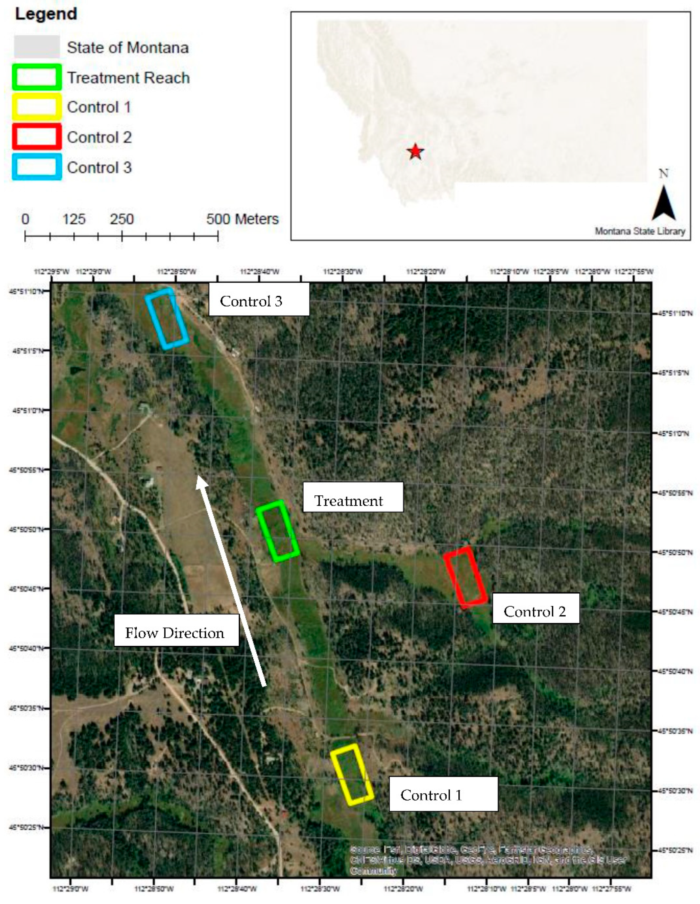
Funding

This work was partly supported by Montana Space Grant Consortium (G106-20-W5472, 2019).

Data Availability Statement

The data presented in this study are available on request from the corresponding author.

Acknowledgments

Montana Bureau of Mines and Geology and Montana Technological University made significant contributions in equipment and data collection. The authors would like to thank landowners for permission to access the study reaches. The authors would also like to thank Kumar Ganesan for his feedback on the manuscript and Amy Chadwick (Great West Engineering, Helena, Montana) who installed the BDAs.

Conflicts of Interest

The authors declare no conflict of interest.

Appendix A

Figure A1. ArcMap flow diagram for EVI values computation (for satellite data only). Blue ovals refer to corresponding reflectance band raster files, treatment, and control clips. The yellow rectangles refer to ArcMap tools. The green ovals refer to output of the products.
Remotesensing 14 06199 g0a1
Figure A2. GCPs and CPs locations for treatment reach and control reach.
Remotesensing 14 06199 g0a2

Appendix B

Comparison of sUAS Red Band Reflectance Values

The sUAS multispectral dual camera system captures two different wavelength ranges for the red band. The RedEdge-MX Blue camera captures from 0.642 to 0.658 µm and the RedEdge-MX camera captures from 0.661 to 0.675 µm. These red reflectance values were compared with Sentinel-2 red band reflectance to determine if combination of the two red multispectral bands was necessary. A percent change analysis was carried out for the control reach 1 on May 10, 2020, between the Sentinel-2 Red band and the sUAS red band from the RedEdge-MX to the Sentinel-2 red band and the average of the two dual camera system red bands (Table 8 and Figure 12). A paired t-test revealed that there is no significant difference (p = 0.817) in reflectance values when using Rededge-MX and combined RedEdge-MX and RedEdge Blue for the red bandwidth. As there is no significant difference, further analysis was conducted using only the RedEdge-MX red band.

References

  1. Barnett, T.P.; Pierce, D.W.; Hidalgo, H.G.; Bonfils, C.; Santer, B.D.; Das, T.; Bala, G.; Wood, A.W.; Nozawa, T.; Mirin, A.A.; et al. Human-Induced Changes in the Hydrology of the Western United States. Science 2008, 319, 1080–1083. [Google Scholar] [CrossRef] [PubMed] [Green Version]
  2. Elias, E.; James, D.; Heimel, S.; Steele, C.; Steltzer, H.; Dott, C. Implications of observed changes in high mountain snow water storage, snowmelt timing and melt window. J. Hydrol. Reg. Stud. 2021, 35, 100799. [Google Scholar] [CrossRef]
  3. Vanderhoof, M.K.; Burt, C. Applying High-Resolution Imagery to Evaluate Restoration-Induced Changes in Stream Condition, Missouri River Headwaters Basin, Montana. Remote Sens. 2018, 10, 913. [Google Scholar] [CrossRef] [Green Version]
  4. Pilliod, D.S.; Rohde, A.T.; Charnley, S.; Davee, R.R.; Dunham, J.B.; Gosnell, H.; Grant, G.E.; Hausner, M.B.; Huntington, J.L.; Nash, C. Survey of Beaver-related Restoration Practices in Rangeland Streams of the Western USA. Environ. Manag. 2017, 61, 58–68. [Google Scholar] [CrossRef] [PubMed]
  5. Fairfax, E.; Small, E.E. Using remote sensing to assess the impact of beaver damming on riparian evapotranspiration in an arid landscape. Ecohydrology 2018, 11, e1993. [Google Scholar] [CrossRef]
  6. Silverman, N.L.; Allred, B.W.; Donnelly, P.; Chapman, T.B.; Maestas, J.; Wheaton, J.; White, J.; Naugle, D.E. Low-tech riparian and wet meadow restoration increases vegetation productivity and resilience across semiarid rangelands. Restor. Ecol. 2018, 27, 269–278. [Google Scholar] [CrossRef] [Green Version]
  7. Lautz, L.; Kelleher, C.; Vidon, P.; Coffman, J.; Riginos, C.; Copeland, H. Restoring stream ecosystem function with beaver dam analogues: Let’s not make the same mistake twice. Hydrol. Process. 2018, 33, 174–177. [Google Scholar] [CrossRef] [Green Version]
  8. DaVee, R.; Gosnell, H.; Charnley, S. Using beaver dam analogues for fish and wildlife recovery on public and private rangelands in eastern Oregon. 2019. Available online: https://www.fs.usda.gov/research/treesearch/58234 (accessed on 22 July 2020).
  9. Wegener, P.; Covino, T.; Wohl, E. Beaver-Mediated Lateral Hydrologic Connectivity, Fluvial Carbon and Nutrient Flux, and Aquatic Ecosystem Metabolism. Water Resour. Res. 2017, 53, 4606–4623. [Google Scholar] [CrossRef]
  10. Scamardo, J.; Wohl, E. Sediment storage and shallow groundwater response to beaver dam analogues in the Colorado Front Range, USA. River Res. Appl. 2020, 36, 398–409. [Google Scholar] [CrossRef]
  11. Loheide, S.P.; Gorelick, S.M. Riparian hydroecology: A coupled model of the observed interactions between groundwater flow and meadow vegetation patterning. Water Resour. Res. 2007, 43, 7. [Google Scholar] [CrossRef]
  12. Tague, C.; Valentine, S.; Kotchen, M. Effect of geomorphic channel restoration on streamflow and groundwater in a snowmelt-dominated watershed. Water Resour. Res. 2008, 44. [Google Scholar] [CrossRef] [Green Version]
  13. Majerova, M.; Neilson, B.T.; Schmadel, N.M.; Wheaton, J.M.; Snow, C.J. Impacts of beaver dams on hydrologic and temperature regimes in a mountain stream. Hydrol. Earth Syst. Sci. 2015, 19, 3541–3556. [Google Scholar] [CrossRef] [Green Version]
  14. Pollock, M.M.; Beechie, T.J.; Wheaton, J.; Jordan, C.E.; Bouwes, N.; Weber, N.; Volk, C. Using Beaver Dams to Restore Incised Stream Ecosystems. Bioscience 2014, 64, 279–290. [Google Scholar] [CrossRef] [Green Version]
  15. Nash, C.S.; Selker, J.S.; Grant, G.E.; Lewis, S.L.; Noël, P. A physical framework for evaluating net effects of wet meadow restoration on late-summer streamflow. Ecohydrology 2018, 11, e1953. [Google Scholar] [CrossRef]
  16. Pflugmacher, D.; Cohen, W.B.; Kennedy, R.E. Using Landsat-derived disturbance history (1972–2010) to predict current forest structure. Remote Sens. Environ. 2012, 122, 146–165. [Google Scholar] [CrossRef]
  17. Eliu, P. A survey of remote-sensing big data. Front. Environ. Sci. 2015, 3, 45. [Google Scholar] [CrossRef] [Green Version]
  18. Ramsey, E.W., III; Laine, S.C. Comparison of Landsat thematic mapper and high-resolution photography to identify change in complex coastal wetlands. J. Coast. Res. 1997, 13, 281–292. [Google Scholar]
  19. Wang, Y.; Colby, J.D.; Mulcahy, K.A. An efficient method for mapping flood extent in a coastal floodplain using Landsat TM and DEM data. Int. J. Remote. Sens. 2002, 23, 3681–3696. [Google Scholar] [CrossRef]
  20. Jarchow, C.J.; Nagler, P.L.; Glenn, E.P. Greenup and evapotranspiration following the Minute 319 pulse flow to Mexico: An analysis using Landsat 8 Normalized Difference Vegetation Index (NDVI) data. Ecol. Eng. 2017, 106, 776–783. [Google Scholar] [CrossRef]
  21. Bhatnagar, S.; Gill, L.; Regan, S.; Naughton, O.; Johnston, P.; Waldren, S.; Ghosh, B. Mapping vegetation communities inside wetlands using Sentinel-2 imagery in Ireland. Int. J. Appl. earth Obs. Geoinf. ITC J. 2020, 88, 102083. [Google Scholar] [CrossRef]
  22. NIAS. The Evolution of Commercial Drone Technology—NIAS-Airspace. 2018. Available online: https://nias-uas.com/evolution-commercial-drone-technology/ (accessed on 22 July 2020).
  23. Melville, B.; Fisher, A.; Lucieer, A. Ultra-high spatial resolution fractional vegetation cover from unmanned aerial multispectral imagery. Int. J. Appl. earth Obs. Geoinf. ITC J. 2019, 78, 14–24. [Google Scholar] [CrossRef]
  24. Norman, E. Hydrologic Response of Headwater Streams Restored with Beaver Dam Analogue Structures. Ph.D. Thesis, Montana Technological University, 2020. Available online: https://digitalcommons.mtech.edu/grad_rsch/239/ (accessed on 1 October 2022).
  25. Schignel. Formula for Enhanced Vegetation Index (EVI) in Raster Calculator. 2017. Available online: https://community.esri.com/thread/69192 (accessed on 1 October 2022).
  26. Glenn, E.P.; Nagler, P.L.; Huete, A.R. Vegetation Index Methods for Estimating Evapotranspiration by Remote Sensing. Surv. Geophys. 2010, 31, 531–555. [Google Scholar] [CrossRef]
  27. Basin Creek SNOWTEL Data. Available online: https://wcc.sc.egov.usda.gov/nwcc/site?sitenum=315 (accessed on 1 December 2022).
  28. Copernicus Sentinel Data. 2020. Available online: https://scihub.copernicus.eu/dhus/#/home (accessed on 5 December 2022).
  29. Copernicus EO Support, Personal Communication. 2020. Available online: https://www.copernicus.eu/en (accessed on 1 October 2022).
  30. McKenzie, N.J.; Sparrow, A.D.; Guerschman, J.P. The Role of Remote Sensing in Agricultural Development and Poverty Alleviation—The STARS Landscaping Study; CSIRO Australia/ITC at the University of Twente: Canberra, Australia, 2016. [Google Scholar]
  31. ESA. 2020. Available online: https://step.esa.int/main/download/snap-download/ (accessed on 5 December 2022).
  32. ESA. 2000–2020. Spatial—Resolutions—Sentinel-2 MSI—User Guides—Sentinel Online. Available online: https://sentinel.esa.int/web/sentinel/user-guides/sentinel-2-msi/resolutions/spatial (accessed on 4 June 2020).
  33. MicaSense, Inc. Dual Camera Imaging System. 2020. Available online: https://micasense.com/dual-camera-system/?utm_term=micasense+dual (accessed on 4 June 2020).
  34. Pix4Dcapture. 2022. Available online: https://www.pix4d.com/product/pix4dcapture (accessed on 1 December 2022).
  35. Ullman, S. The Interpretation of Structure from Motion. Proc. R. Soc. London. Ser. B Biol. Sci. 1979, 203, 405–426. [Google Scholar]
  36. Pix4Dmapper. 2022. Available online: https://support.micasense.com/hc/en-us/articles/115000831714-How-to-Process-MicaSense-Sensor-Data-in-Pix4D (accessed on 1 December 2022).
  37. Jiang, Z.; Huete, A.R.; Kim, Y.; Didan, K. 2-band enhanced vegetation index without a blue band and its application to AVHRR data. Remote Sens. Modeling Ecosyst. Sustain. IV 2007, 6679, 667905. [Google Scholar] [CrossRef]
  38. Matsushita, B.; Yang, W.; Chen, J.; Onda, Y.; Qiu, G. Sensitivity of the Enhanced Vegetation Index (EVI) and Normalized Difference Vegetation Index (NDVI) to Topographic Effects: A Case Study in High-density Cypress Forest. Sensors 2007, 7, 2636–2651. [Google Scholar] [CrossRef] [PubMed] [Green Version]
  39. Huete, A.; Didan, K.; Miura, T.; Rodriguez, E.P.; Gao, X.; Ferreira, L.G. Overview of the radiometric and biophysical performance of the MODIS vegetation indices. Remote Sens. Environ. 2002, 83, 195–213. [Google Scholar] [CrossRef]
  40. Nagler, P.L.; Glenn, E.P.; Nguyen, U.; Scott, R.L.; Doody, T. Estimating Riparian and Agricultural Actual Evapotranspiration by Reference Evapotranspiration and MODIS Enhanced Vegetation Index. Remote Sens. 2013, 5, 3849–3871. [Google Scholar] [CrossRef] [Green Version]
  41. Nagler, P.L.; Barreto-Muñoz, A.; Borujeni, S.C.; Nouri, H.; Jarchow, C.J.; Didan, K. Riparian Area Changes in Greenness and Water Use on the Lower Colorado River in the USA from 2000 to 2020. Remote Sens. 2021, 13, 1332. [Google Scholar] [CrossRef]
  42. Abbasi, N.; Nouri, H.; Didan, K.; Barreto-Muñoz, A.; Borujeni, S.C.; Salemi, H.; Opp, C.; Siebert, S.; Nagler, P. Estimating Actual Evapotranspiration over Croplands Using Vegetation Index Methods and Dynamic Harvested Area. Remote Sens. 2021, 13, 5167. [Google Scholar] [CrossRef]
  43. Allen, R.G.; Walter, I.A.; Elliott, R.; Howell, T.A.; Itenfisu, D.; Jensen, M.E. The ASCE Standardized Reference Evapotranspiration Equation; American Society of Civil Engineers: New York, NY, USA, 2005; p. 216. [Google Scholar]
Figure 1. Study Reach Locations.
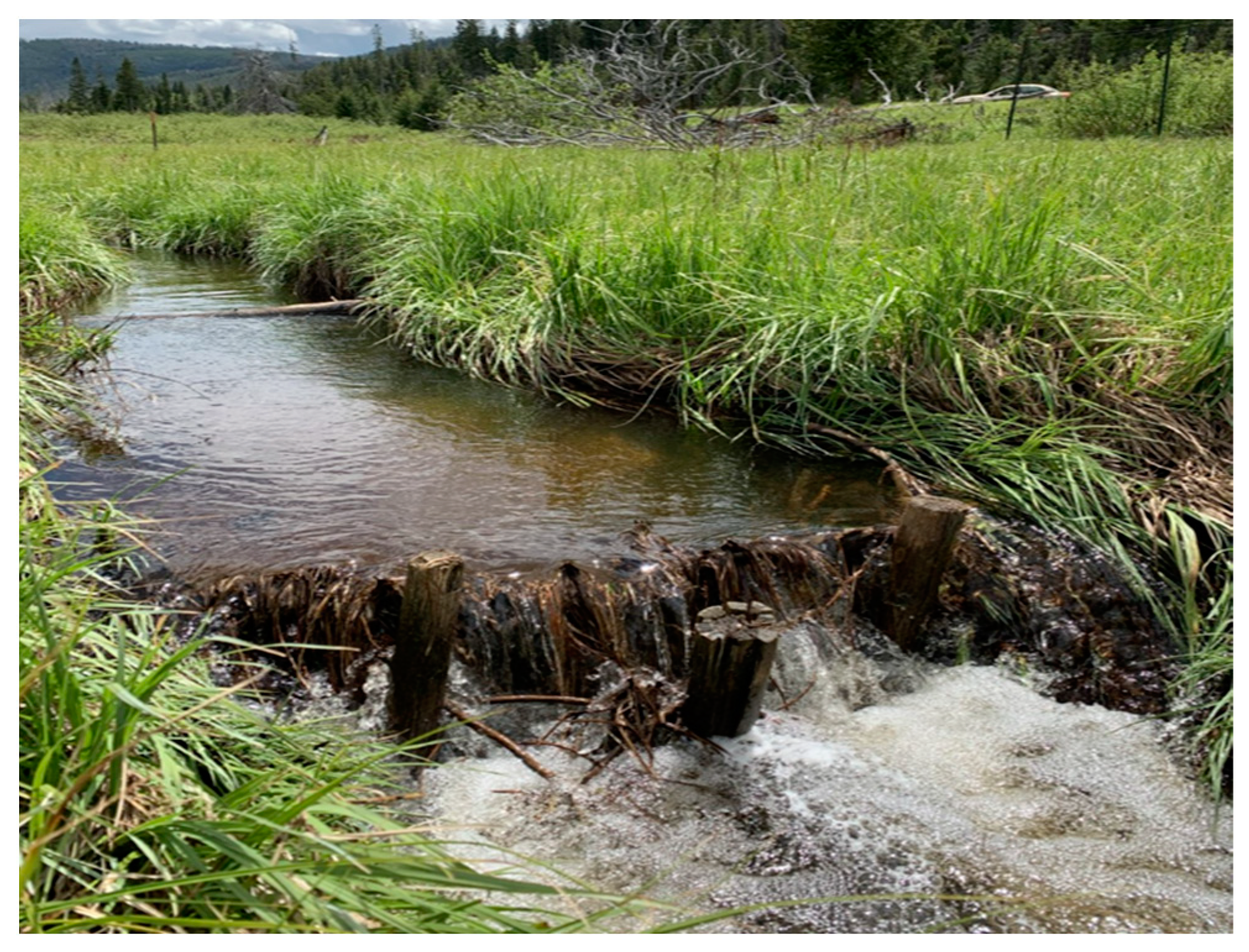
Remotesensing 14 06199 g001
Figure 2. Typical BDA restoration configuration. Photos taken post-treatment (19 June 2020).
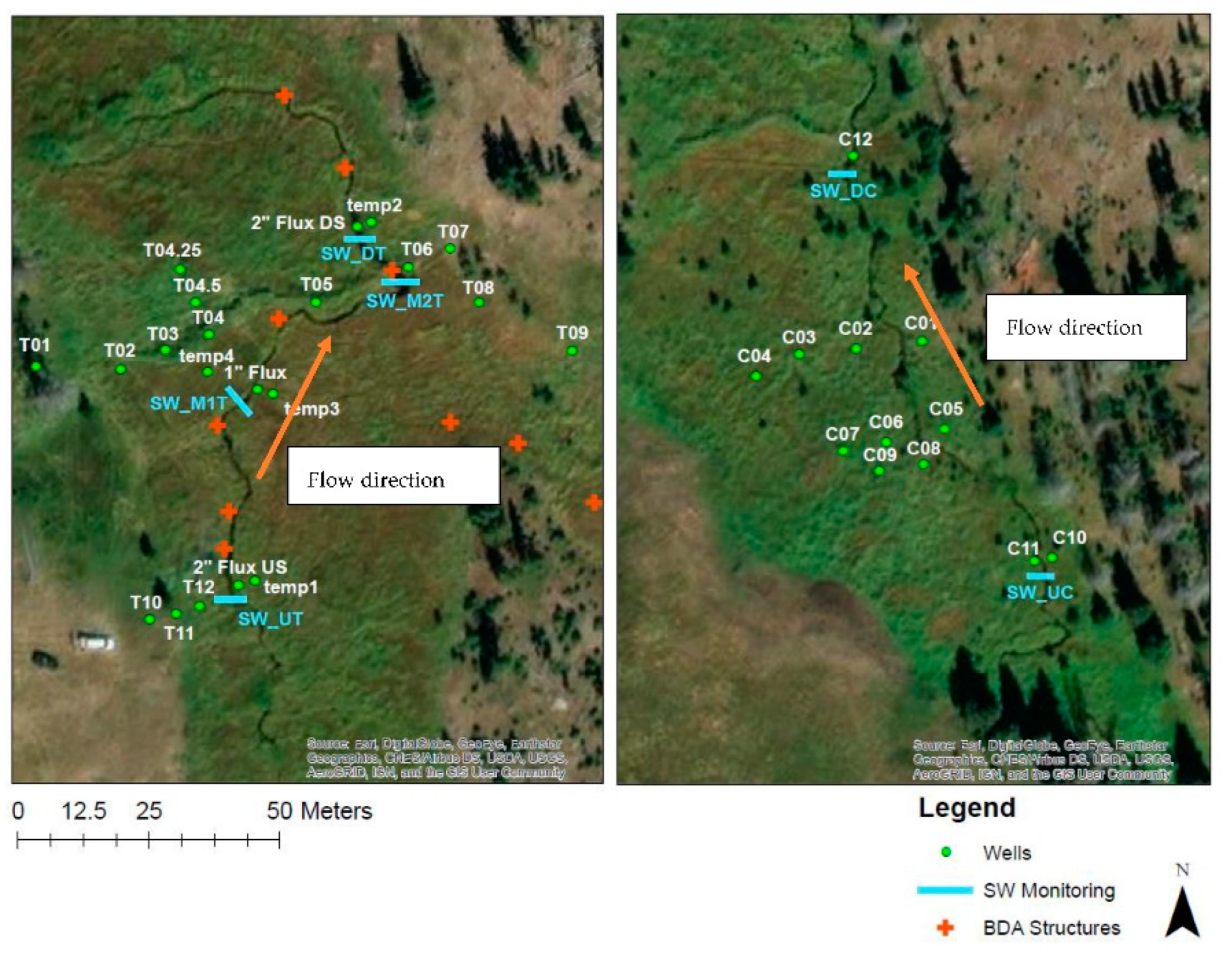
Remotesensing 14 06199 g002
Figure 3. Groundwater and surface water monitoring locations. (Left) Treatment reach. (Right) Control 1 reach.
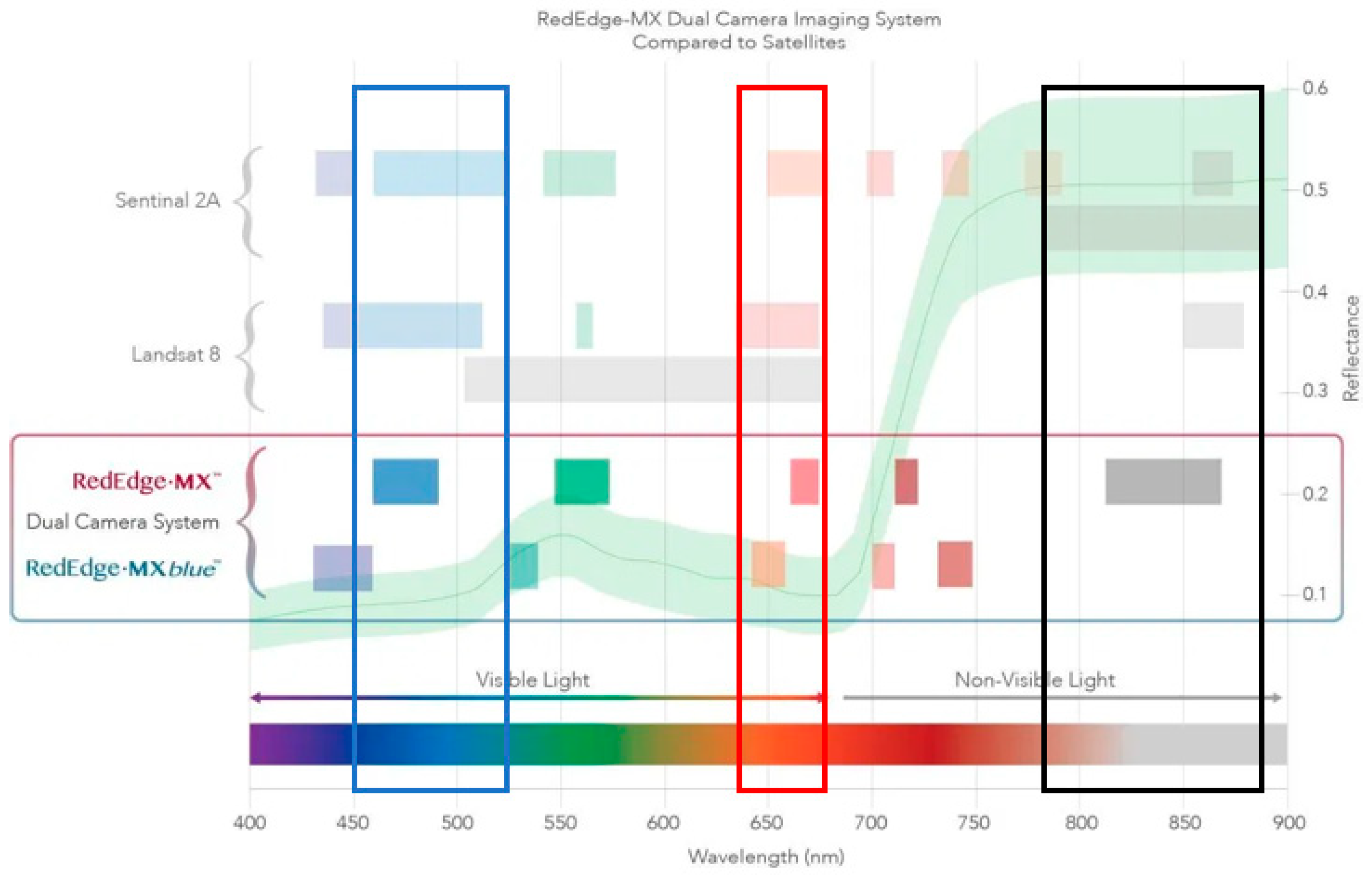
Remotesensing 14 06199 g003
Figure 4. Spectral reflectance band comparison of dual camera system with Landsat 8 and Sentinel-2 (used with permission from MicaSense, Inc., Seattle, WA, USA). Colored boxes represent blue, red, and NIR wavelengths for each imaging system.
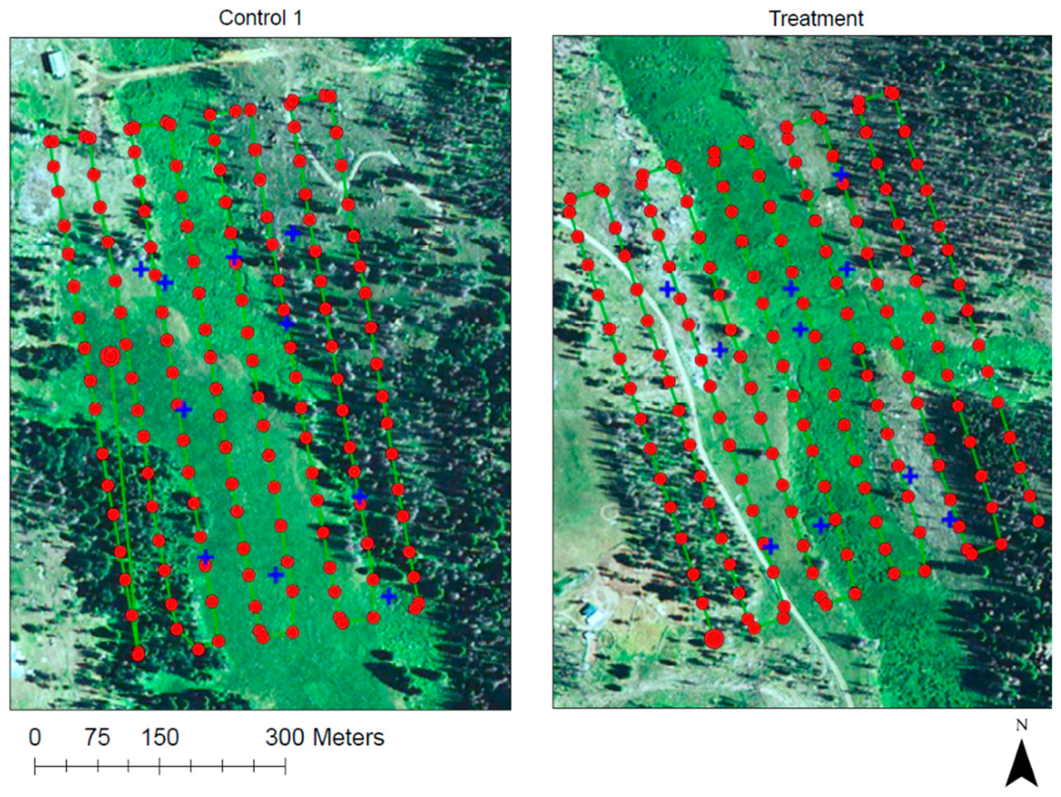
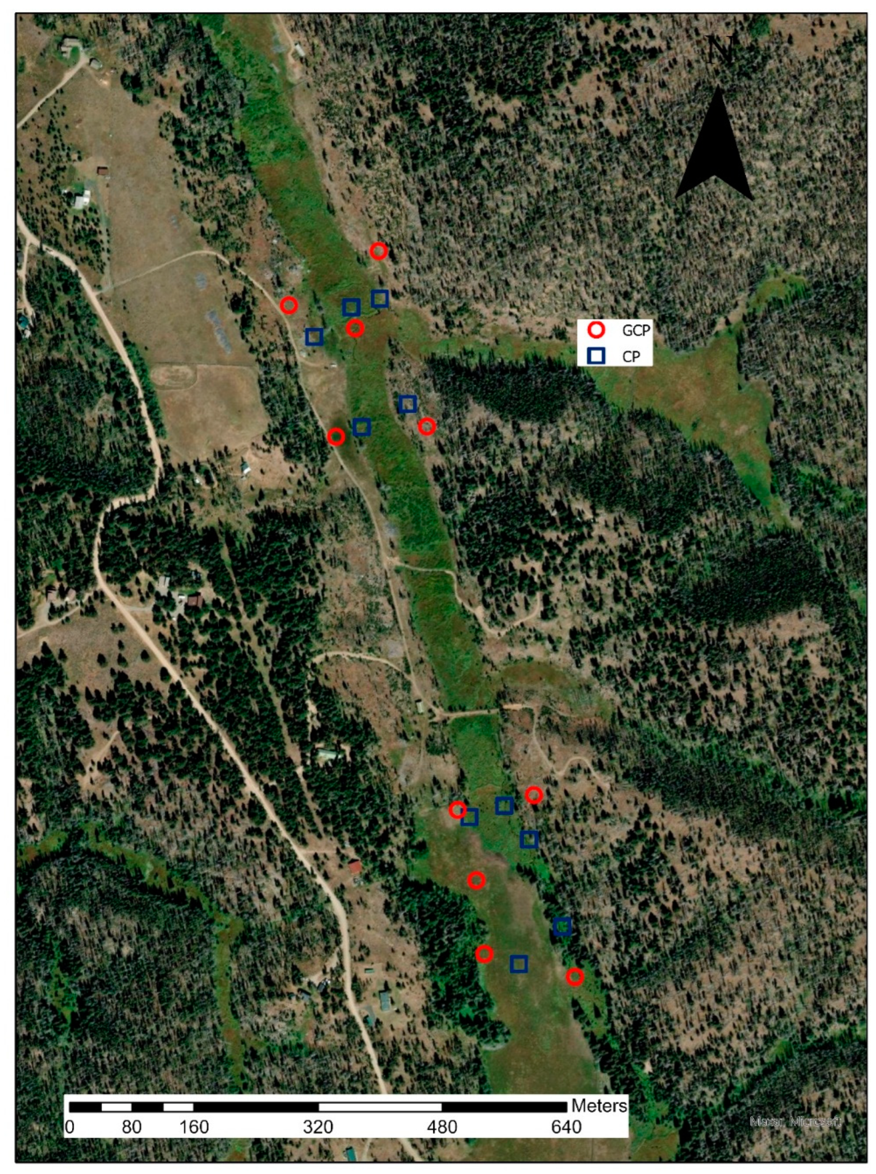
Remotesensing 14 06199 g004
Figure 5. sUAS flight paths. Red dots represent individual captures and blue crosshairs represent geolocated ground control points and check points. (Left): Control 1 reach. (Right): Treatment reach.
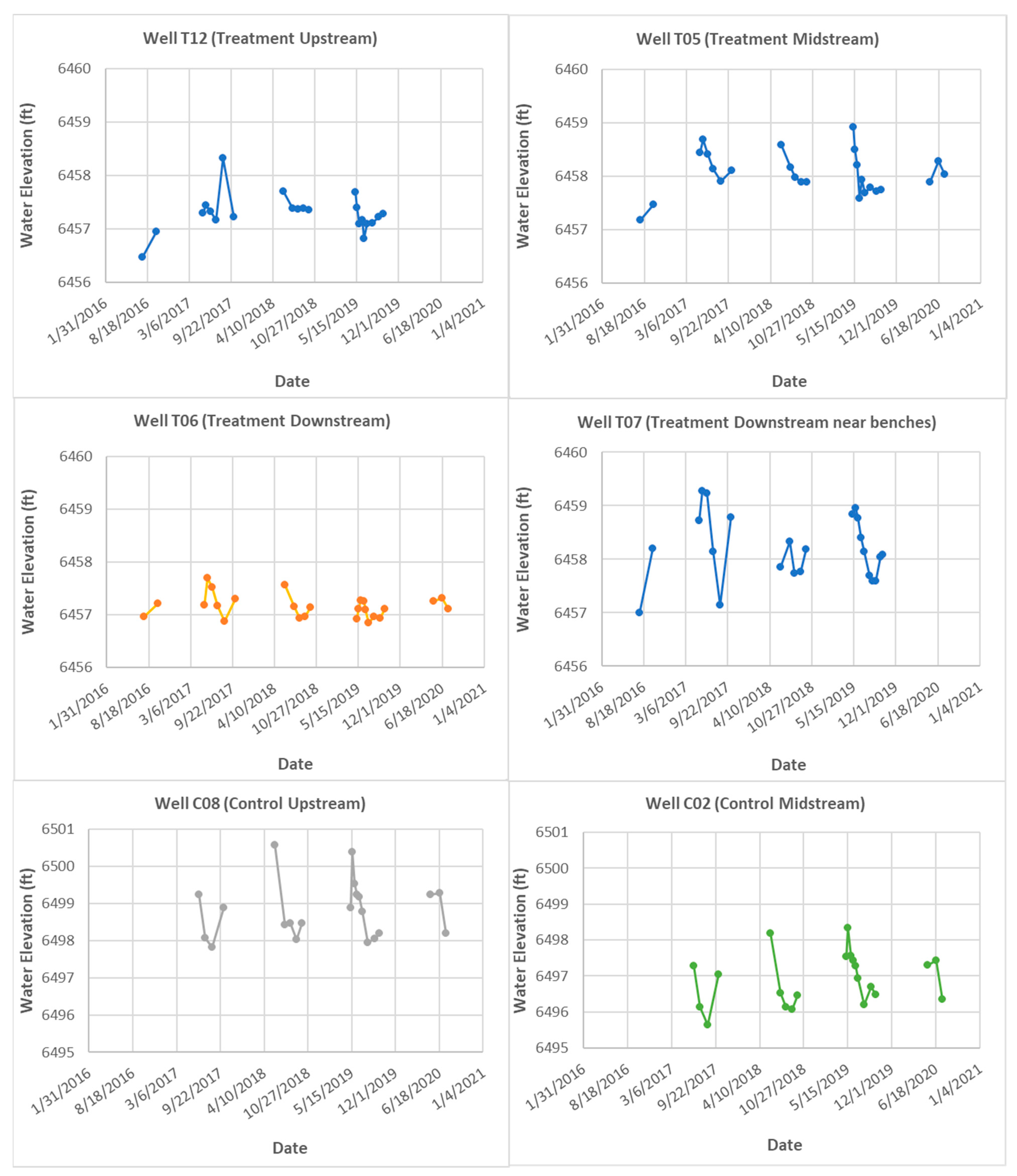
Remotesensing 14 06199 g005
Figure 6. Groundwater elevations for wells in the treatment and control reaches on Blacktail Creek (data up to year 2019 are from Norman [24]; 2020 data are collected as part of this study).
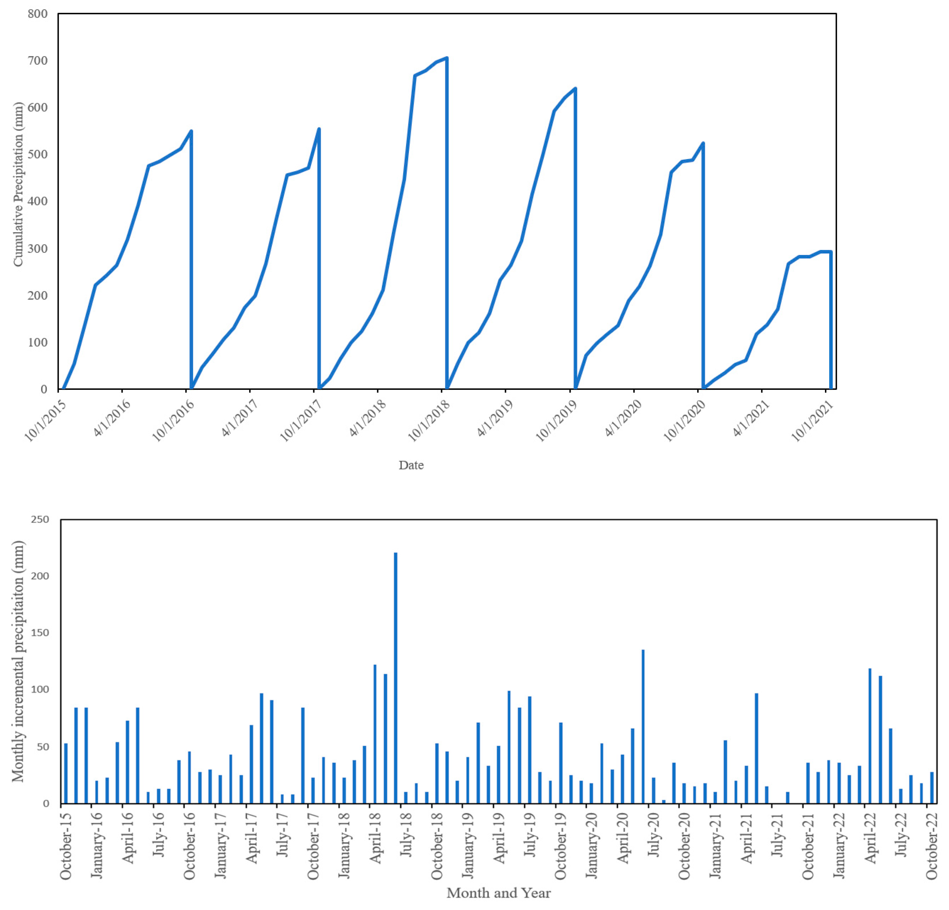
Remotesensing 14 06199 g006
Figure 7. Basin Creek SNOWTEL station precipitation data. Top–Water year cumulative precipitation data (cumulative for water year beginning 1 October and ending 30 September). Bottom–Monthly incremental precipitation values.
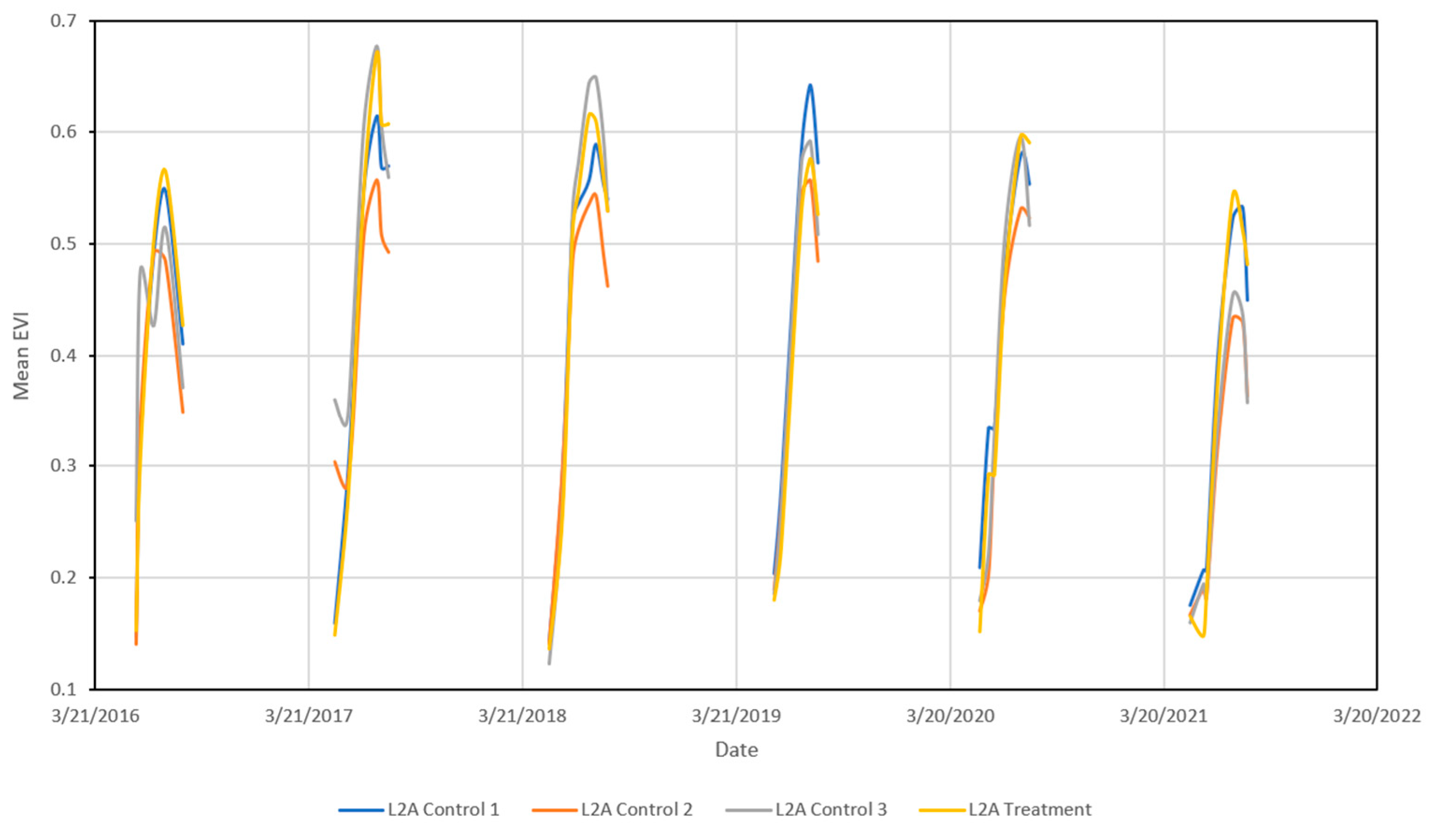
Remotesensing 14 06199 g007
Figure 8. Sentinel-2 (May to August, 2016–2021) mean EVI values (level-2A, dimensionless) for treatment and control reaches.
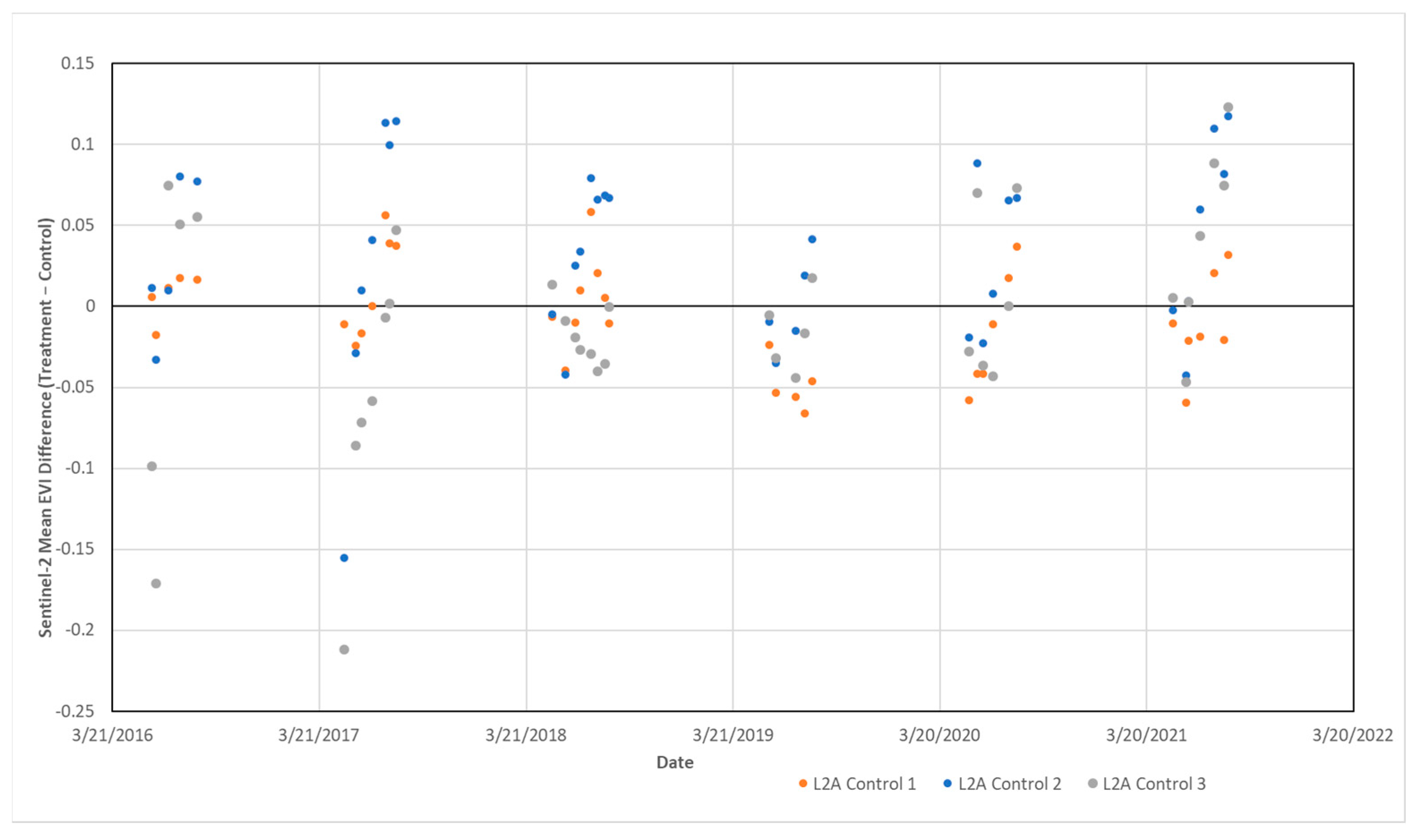
Remotesensing 14 06199 g008
Figure 9. Sentinel-2 mean EVI difference (Treatment–Control, dimensionless) values.
Remotesensing 14 06199 g009
Figure 10. Sentinel-2 mean EVI difference (Treatment–Control, dimensionless) values for the month of August (dry season, when changes in water availability would be most apparent).
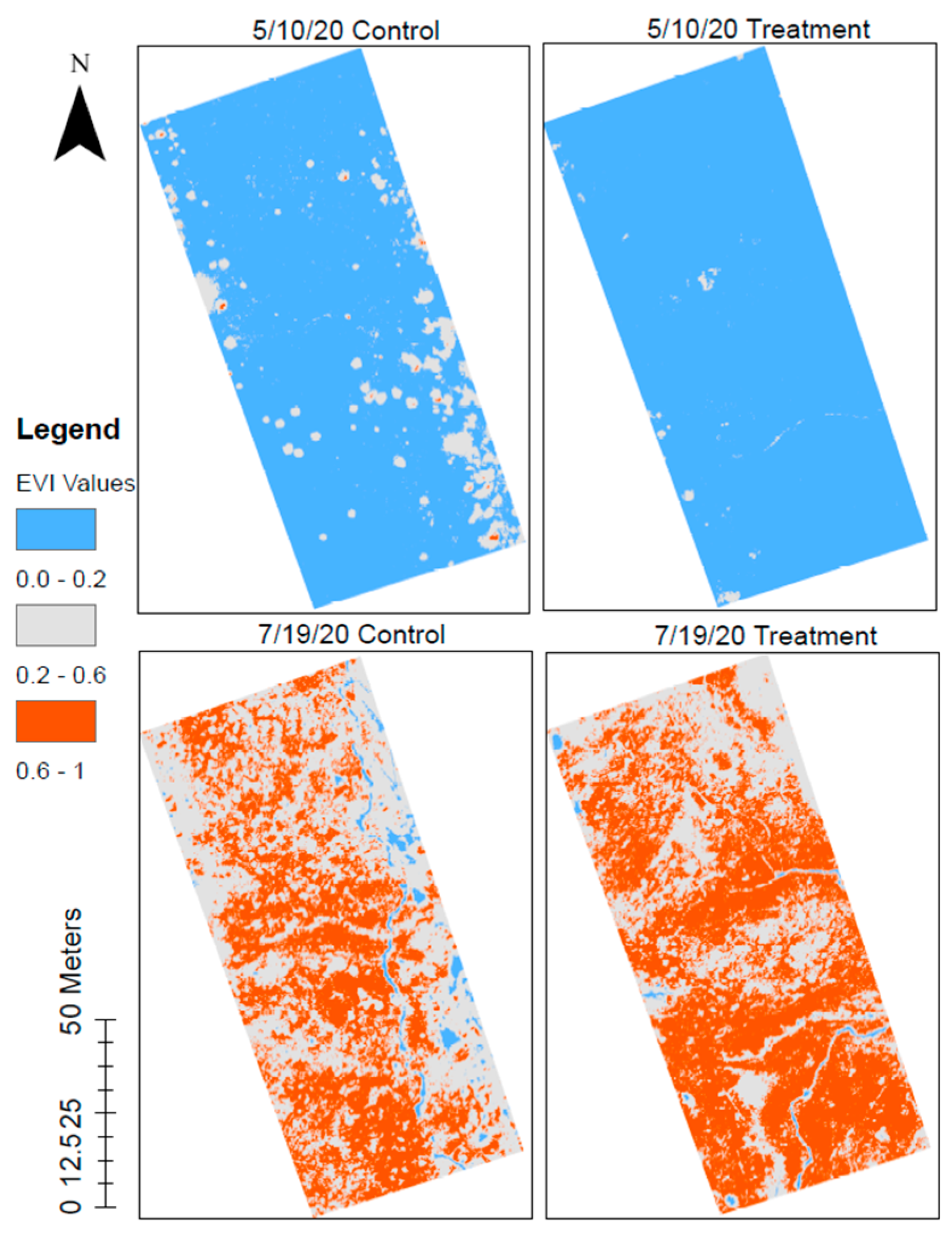
Remotesensing 14 06199 g010
Figure 11. Spatial and temporal variation of EVI values in the study reach and control 1 reach.
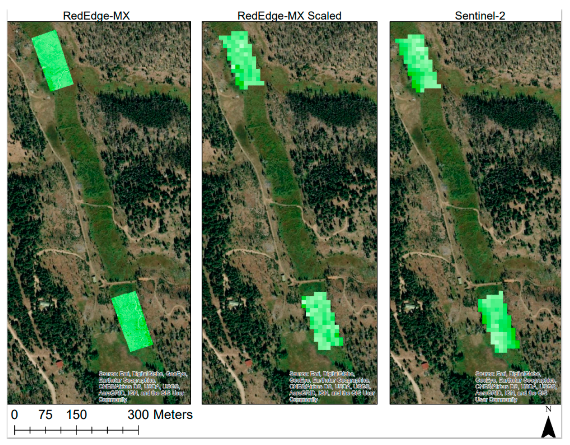
Remotesensing 14 06199 g011
Figure 12. EVI raster images from Sentinel-2, RedEdge-MX dual camera system and scaled RedEdge-MX for treatment reach on 25 May 2020.
Remotesensing 14 06199 g012
Table 1. Abbreviations and symbols.
Abbreviations and SymbolsMeaning
AMSLAbove Mean Sea Level
BDAsBeaver Dam Analogs
CPsCheck points
ETEvapotranspiration
ETaActual evapotranspiration
EToLocal reference crop evapotranspiration
EVIEnhanced Vegetation Index
EVImax99.5 percentile value of the EVI data
EVImin0.5 percentile value of the EVI data
EVI* Rescaled EVI values
GCPsGround control points
NIR Near Infrared
SfMStructure from Motion
sUASsmall Unmanned Aerial System
Table 2. Wavelengths for Sentinel-2 and sUAS [32,33] remote sensing. NA refers to the cells where the sensor is not designed to collect the corresponding bandwidth data.
Sentinel-2Dual Camera System 1
Band 1Coastal Aerosol (0.433–0.453)Blue (0.459–0.491 µm)
Band 2Blue (0.458–0.522)Green (0.547–0.574 µm)
Band 3Green (0.543–0.577)Red (0.661–0.675 µm)
Band 4Red (0.65–0.68)Red Edge (0.711–0.723 µm)
Band 5Vegetation Red Edge (0.698–0.712)NIR (0.814–0.871 µm)
Band 6Vegetation Red Edge (0.733–0.747)Coastal Blue (MX Blue) (0.430–0.458 µm)
Band 7Vegetation Red Edge (0.773–0.793)Green (MX Blue) (0.524–0.538 µm)
Band 8NIR (0.785–0.899)Red (MX Blue) (0.642–0.658 µm
Band 8aVegetation Red Edge (0.855–0.875)NA
Band 9Water vapor (0.935–0.955)Red Edge 1 (MX Blue) (0.700–0.710 µm
Band 10SWIR-Cirrus (1.36–1.39)Red Edge 2 (MX Blue) (0.731–0.749 µm)
Band 11SWIR (1.565–1.655)NA
Band 12SWIR (2.1–2.28)NA
1 DJI Matrice 600 Pro with a MicaSense RedEdge-MX and RedEdge-MX Blue multispectral cameras.
Table 3. Streamflow measurements for control 1 and treatment reaches (Figure 3).
Control10 May 202019 June 202019 July 202023 August 2020Treatment10 May 202019 June 202019 July 202023 August 2020
NameFlow (m3/s) Flow (m3/s) Flow (m3/s) Flow (m3/s) NameFlow (m3/s) Flow (m3/s) Flow (m3/s) Flow (m3/s)
SW_UC 0.0540.1130.0300.017SW_UT0.0450.1020.0320.018
SW_DC 0.0500.1050.0310.023SW_M1T0.0580.0980.0370.016
SW_M2T0.0600.1290.0440.016
SW_DT0.0620.1410.0450.015
Table 4. Statistics for sUAS multispectral flights: sample size (n) and root mean square error (x, y, and z) in geolocation of multispectral products for ground control points (GCP) and check points (CP).
DateStudy LocationGround Sampling Distance (cm)RMSE for GCPsRMSE for CPs
nX (cm)Y (cm)Z (cm)nX (cm)Y (cm)Z (cm)
10 May 2020Control852115536
Treatment851125319
19 July 2020Control9 521253414
Treatment8511154119
Table 5. Summary of images processed, area covered, median keypoints per image, calibrated images, and median matches per image for sUAS multispectral orthomosaic.
DateStudy LocationNumber of Images Area Covered (ha)Median Keypoints Per ImageCalibrated ImagesMedian Matches Per Calibrated Image
10 May 2020Control74012.510,000100%5651
Treatment82012.510,00098%5922
19 July 2020Control71512.610,000100%5062
Treatment82014.010,000100%5186
Table 6. Comparison of EVI values, calculated using ArcMap, between the RedEdge-MX, the RedEdge-MX pixel scaled to 10 m, and Sentinel-2 Level-2A data for 10 May 2020 and 19 July 2020.
RedEdge-MXRedEdge-MX ScaledSentinel-2
ControlRestoredControlRestoredControlRestored
10 May 2020Minimum−0.013−0.0140.0450.0250.1550.125
Maximum0.7150.5760.5300.2130.3030.171
Mean 0.1520.1210.1480.1190.2090.151
Std. Dev.0.0690.0250.0610.0260.0330.009
19 July 2020Minimum0.036−0.0260.2020.2020.4360.505
Maximum0.9010.9470.8230.8350.6670.667
Mean 0.5520.6100.5650.6050.5790.596
Std. Dev.0.1360.1140.1360.1000.0610.036
Table 7. EVImax, EVImin, and ETo, for sUAS flights on 10 May 2020 and 19 July 2020.
ControlTreatment
10 May 2020EVImax (unitless)0.6080.406
EVImin (unitless)0.0190.005
ETo (mm/d)4.44.4
19 July 2020EVImax (unitless)0.8210.859
EVImin (unitless)0.0910.124
ETo (mm/d)4.94.9
Table 8. Descriptive statistics for estimated evapotranspiration values for sUAS flights 10 May 2020 and 19 July 2020.
Evapotranspiration Values (mm/d)
ControlTreatment
10 May 2020Min00
Max5.755.75
Mean2.032.7
19 July 2020Min00
Max6.406.61
Mean5.135.32
Publisher’s Note: MDPI stays neutral with regard to jurisdictional claims in published maps and institutional affiliations.

