Abstract
The Amazon Macrotidal Mangrove Coast contains the most extensive and continuous mangrove belt globally, occupying an area of ~6500 km2 and accounting for 4.2% of global mangroves. The tallest and densest mangrove forests in the Amazon occur on the Bragança Peninsula. However, road construction that occurred in 1973 caused significant mangrove degradation in the area. A spatial-temporal analysis (1986–2019) based on optical, Synthetic Aperture Radar (SAR), drone images, and altimetric data obtained by photogrammetry and validated by a topographic survey were carried out to understand how the construction of a road led to the death of mangroves. The topographic data suggested that this road altered the hydrodynamical flow, damming tidal waters. This process killed at least 4.3 km2 of mangrove trees. Nevertheless, due to natural mangrove recolonization, the area exhibiting degraded mangrove health decreased to ~2.8 km2 in 2003 and ~0.73 km2 in 2019. Climatic extreme events such as “El Niño” and “La Niña” had ephemeral control over the mangrove degradation/regeneration. In contrast, the relative sea-level rise during the last several decades caused long-term mangrove recolonization, expanding mangrove areas from lower to higher tidal flats. Permanently flooded depressions in the study area, created by the altered hydrodynamical flow due to the road, are unlikely to be recolonized by mangroves unless connections are re-established between these depressions with drainage on the Caeté estuary through pipes or bridges to prevent water accumulation between the road and depressions. To minimize impacts on mangroves, this road should have initially been designed to cross mangrove areas on the highest tidal flats and to skirt the channel headwaters to avoid interruption of regular tidal flow.
1. Introduction
Mangroves are a key component of tropical coastal forests, covering 8% (137,700 km2) of the world’s coastal areas [1,2,3,4,5]. Mangrove forests serve as sources, sinks, and transformers of nutrients and organic matter and are one of the most productive ecosystems globally [6]. In addition, these forests perform essential socio-economic and environmental functions, such as coastal sequestration and storage of carbon, conservation of biological diversity, and coastal protection against the effects of storms and inundation by sea-level rise [7,8,9]. However, the equilibrium between mangrove substrates and tidal level is susceptible to sea-level rise [10,11,12]. Global mangrove losses were 1.04% per year from 1980 to 2000 [7] and 0.39% per year from 2000 to 2014, whereby Brazil had a net loss of mangrove coverage of 930 km2 [13]. According to Thomas et al. [14], the main cause of mangrove loss in the world between 1996 and 2010 is the anthropogenic conversion of mangrove forests to land meant for aquaculture/agriculture.
Multi-source remote sensing datasets (e.g., Satellite optical, SAR, or drone) can provide complementary information for mangrove assessment and drivers responsible for degradation and regeneration [15,16,17,18,19]. Landsat mid-resolution satellite datasets provide advantages for historical mangrove analysis due to the availability of their archives since the 1980s [20]. However, Landsat’s coarse spatial resolution is not at a fine enough scale to allow mangrove species monitoring [21]. Therefore, for mangrove species mapping, high-resolution datasets offer a cost-efficient method to obtain detailed information [18,22]. Alternatively, drone-derived data can provide additional canopy height and mangrove substrate topographic information [23,24,25,26], with the advantages of a brief time required to sample mangrove forest areas of low accessibility [27].
The northern Brazilian coast has the most extensive mangrove system globally, with an area of 7590 km2 containing 56% of Brazilian mangroves [28,29]. This region is located in the Amazon Macrotidal Mangrove Coast (AMCC) (Figure 1a), which is a global hotspot of intensive changes in mangrove coverage [14]. The Bragança-PA Peninsula is situated within the AMCC and is covered by an extensive mangrove area (Figure 1b) with tree heights up to 25 m [30]. Degraded mangrove areas are found close to the center of the Bragança Peninsula, on the highest tidal flats [31]. This degradation may be related to the construction of the Bragança-Ajuruteua highway (Highway PA-458) during the 1970s [31,32].
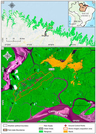
Figure 1.
Study area: (a) Location of the study area in South America; (b) Mangrove coverage in the Amazon Macrotidal Mangrove Coast; (c) Positions of Ground Control Points (GCPs) along the road and degraded mangrove, and drone imagery acquisition in the study area.
Anthropogenic construction in mangrove forests can alter the hydrologic dynamics of the forest and lead to degradation. Shipyards and other nautical structures related to the Santos port degraded 78.4% of mangrove forests in the Beritoga Channel (SP, Brazil) [33]. Sewage accumulation and hydrologic restriction in estuarine tidal channels by concrete gates or industrial buildings produced mangrove dieback in the Colombian Caribbean and the Indian Golden Chemical Corridor of Gujarat [34,35]. Urban development projects for road and bridge construction may cause deviation of supply tidal creeks, blocking channels that feed the mangrove substrate, such as in the Wouri River Estuary (Douala, Cameroon) [36].
Located in the Bragança Peninsula, Highway PA-458 was built along 26 km of dense mangrove forests [37]. Before road construction, the mangrove cover was homogeneous, even in the middle of the peninsula [31,32]. The impacts of the road are not restricted to ecosystem degradation but also socio-economic effects, such as uncontrolled population growth and an increase in demand for fishing and extractive products [38]. An initial study by Cohen and Lara [31] inferred mangrove degradation in the western road sector; however, more recent studies show mangrove forests under stress on both sides [37].
In recent decades, several studies reported the recolonization of degraded mangrove areas, mainly by Avicennia trees on topographically elevated tidal flats [30,31,32,39,40]. This process may be attributed to an increase in the period of tidal inundation related to sea-level rise and climate changes such as variations in rainfall or river discharge [30]. However, some questions about the impacts of PA-458 construction on mangroves remain unanswered: (1) Why did the mangrove degradation occur mainly on the northwest side of the road? (2) How does the highway interfere with the drainage system and affect the physical-chemical properties of the tidal flats? (3) Which factors should have been considered for road construction to minimize the impacts on mangroves? This study answered these questions through a spatial-temporal analysis (1986–2019) based on optical, Synthetic Aperture Radar (SAR), drone images, and altimetric data obtained by photogrammetry and validated by a topographic survey.
2. Materials and Methods
Through mid and high-resolution satellite data, land cover maps were generated to understand mangrove dynamics in the Bragança Peninsula. From the mid-resolution assessment, we defined an area of interest for drone surveying to produce digital elevation models (Figure 2).
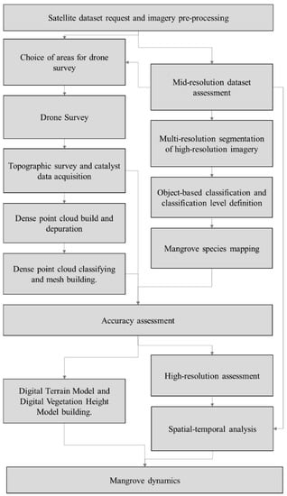
Figure 2.
Methodology flowchart.
2.1. Study Area
The Bragança Peninsula is located in the state of Pará, on the northeastern Brazilian Amazon (Figure 1a), where the intertidal zone is mainly dominated by mangrove and herbaceous flats that occupy ~3090 and ~90 km2, respectively [41]. It is under the influence of the Caeté estuary and Taperaçu channel. The main hydrodynamic feature of the Bragança Peninsula is the tide, with a mean tidal range of 4.5 m [42,43]. The climate is tropical-humid, with a rainy (January to July) and dry season (August to December). The Caeté estuary is subjected mainly to the influence of freshwater discharge; therefore, the porewater salinity in the peninsula will be higher toward the Taperaçu channel [43]. Ecohydrological models based on field datasets with topography, tidal inundation frequency, porewater salinity and vegetation distribution in the Bragança Peninsula were previously published [25,30,31,32]. The porewater salinity in the Bragança Peninsula also depends on estuarine salinity gradients [32] and topography, with the lowest (~30‰) and highest (30–100‰) porewater salinities occurring in the lowest (tidal inundation frequency ~240 days/yr, ~1 m above mean sea-level, amsl) and highest tidal flats (tidal inundation frequency ~240–40 days/yr, 1–4 m amsl), respectively (Figure 3). These porewater salinity gradients affect the mangrove structure [25,30,31,32]. The main mangrove species in the Bragança Peninsula are Rhizophora mangle, and Avicennia germinans, occupying the lowest and highest tidal flats, respectively. Laguncularia occurs in lesser abundance [44]. A database involving the topography and salinity relationship was used to support our interpretations of topographic gradient effects on the vegetation of the study area [25,31].
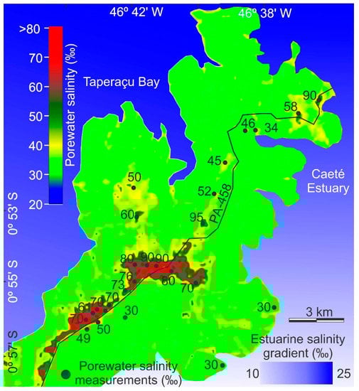
Figure 3.
Sediment porewater salinity in the Bragança Peninsula based on regressions between measured porewater salinities obtained in 2002 and 2017 [30,31], and estuarine salinity gradient (modified from Lara and Cohen [32]).
2.2. Satellite Dataset and Digital Image Processing
This study used optical imagery from Landsat 5 TM (August/1986, October/1993, September/2006, and July/2010), Landsat 7 ETM+ (August/1999), Landsat 8 OLI (December/2015), and Sentinel-2A (September/2019). The imagery was acquired during the dry season, August to December (except the image from 2010 with an acquisition date in the last days of July), to have minimal cloud coverage. SAR data from L-band JERS-1 (acquisition 1993) and ALOS PALSAR (acquisition 2006) complemented cloud-covered regions over the degraded areas. Optical imagery was geometrically corrected using ortho-rectification. Landsat-5 TM imagery was radiometrically corrected through the ATCOR algorithm of the PCI Geomatics software. SAR imagery was calibrated to obtain backscatter values in each pixel, speckle filtered with a 3 × 3 Lee filter to remove the salt-pepper-like texture, and Terrain-Corrected to avoid topographical distortions. According to the availability, we used high-resolution images from Google Earth Pro (~1 m spatial resolution) for 2003; and Pléiades-1 (spatial resolution of 2 m for multispectral and 0.5 m for panchromatic) for 2015, 2017, and 2019. Pléiades-1 data was fused by the Gram–Schmidt spectral sharpening method to produce 0.5 m pan-sharpened imagery.
2.3. Mid-Resolution Classification
To discriminate and quantify the degraded areas in the mid-resolution dataset, the optimal three-band RGB combination selected was: for Landsat 5 TM: 7, 4, 1; for Landsat 7 ETM+: 7, 4, 3; for Landsat 8 OLI: 6, 5, 3; and for Sentinel-2A: 4, 8, 2; chosen through the calculation of the Optimum Index Factor. Using these RGB compositions as a base, visual interpretation methods allowed for individualizing the degraded areas. Due to differences in the backscattering response from degraded areas (smooth specular backscattering) and the vegetation (rough volume backscattering) in SAR imagery, scenes with high cloud coverage (Landsat-5 1993 and 2006) could be mapped. It increased the accuracy of mangrove degradation estimates in cloudy images.
2.4. High-Resolution Image Classification
Mangroves were classified following a three-level hierarchy proposed by Wang et al. [45]. This hierarchy was adapted for each sensor following the decision tree defined in Table 1. For level 1, we described five classes (1) clouds, (2) construction land and other anthropogenically impacted lands, (3) degraded mangrove, (4) vegetation, and (5) water; level 2 separates mangrove from non-mangrove vegetation, and level 3 differentiates the mangrove species Avicennia and Rhizophora. Levels 1 and 2 were carried out through a Geographic Object-Based Image Analysis (GEOBIA) (Figure 4). The paucity of Laguncularia trees scattered among the Avicennia and Rhizophora trees did not allow for their individualization. The classification algorithm used for land cover prediction was the Nearest Neighbor, part of the eCognition object-oriented paradigm. It assigns each object to the class closest to it in the feature space. This method is based on segmentation, dividing the image into meaningful, spatially continuous, and spectrally homogeneous objects or pixel groups [46,47]. The segmentation process was conducted in the eCognition 9.0 software by its multiresolution segmentation algorithm, which several studies have tested for land use and mangrove classification, e.g., [29,45,46,47,48]. Parameters for segmentation (scale, shape, compactness, and band weights) and band names for each dataset are in Table 1. At level 1 for the Pleiades dataset, two normalized difference indices were calculated, one for water (NDWI, Equation (1)) and the other for vegetation (NDVI, Equation (2)).
where Green, Red, and NIR represent the atmospheric reflectance for each band channel.

Table 1.
Parameter settings for multi-resolution segmentation (segmentation scale, shape, compactness, and band weights) of high-resolution datasets.
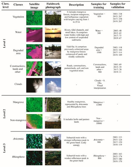
Figure 4.
Description of high-resolution classification in this study.
Every object with NDWI values greater than zero was classified as water, and objects with NDVI values greater than 0.5 were classified as vegetation. Cloud class was manually interpreted. A multiresolution classification was carried out using spectral and geometrical features of objects to individualize the level 1 classes. At level 2, only spectral parameters were considered to separate mangrove from non-mangrove vegetation. NDVI and NIR bands showed to be especially useful in differentiating mangroves from other vegetation units due to the low overlap of the samples collected to train the multiresolution classification model. At level 3, the mangrove species classifications were performed within the mangrove mask. For multiresolution classification, three kinds of object features were selected: spectral (mean value of four layers R/G/B/NIR, brightness, and NDVI), geometrical (shape index), and textural (contrast, entropy, and correlation). The Google Earth Pro dataset did not include spectral parameters such as mean values of NIR, NDVI, and NDWI or texture features (Table 1). Therefore, a higher visual examination and manual edition were carried out to produce more precise results for this dataset, especially at levels 2 and 3.
Two spatiotemporal landcover change analyses were performed, recognizing the classes conversion for the classifications between the 2003 and 2019 scenes. The first analysis is based on the mangrove mask from classification level 2 of 2003, compared against the classes from level 1 (except the vegetation class) of 2019, producing four landcover change classes: stable mangrove, mangrove gain, mangrove retreat, and remaining degraded area. The second landcover change analysis was based on the degraded area class from the 2003 scene, compared against the level 2 and 3 classes from 2019; five landcover change classes were defined: Avicennia colonization, Rhizophora colonization, incipient mangrove, and remaining degraded area.
2.5. High-Resolution Classification Accuracy
The thematic maps, obtained by visual interpretation of the high-resolution dataset, were validated through accuracy assessment. To avoid challenges and uncertainties that represent polygon sampling, such as the lack of polygons from higher-resolution reference data and difficulties in polygon borders creation in the field [49], we opted for point samples. This approach provides an area-based accuracy, assessing the classification by a confusion matrix. To define the point samples, we used the “Create Accuracy Assessment Points” tool from ArcGIS Pro to generate 475 randomly stratified points, where each class has points proportional to its relative area in the imagery (Figure 4) [50]. Overall accuracy, user’s and producer’s accuracy, Kappa overall index, and per class [51]; allocation disagreement (AD), and quantity disagreement (QD) [52] were calculated as a product of the confusion matrix.
2.6. Drone Imagery Acquisition and Processing
An ortho-mosaic was created from aerial photographs obtained from a Drone Phantom 4. This drone has an FC 330 digital 4 K/12MP (Table 2). The Inertial Measurement Unit (IMU) and compass were calibrated once a day before the missions. The camera is positioned on a motion-compensated gimbal. The camera and vision sensors were calibrated by the DJI Assistant 2 software, allowing the production of orthoimages with Ground Sampling Distance (GSD, Equation (3)) of 4.17 (100 m altitude), 3.34 (80 m), and 2.5 cm/pixel (60 m).
where SW is the sensor width of the camera (millimeters), H is the flight height (meters), Fr is the focal length of the camera (millimeters) and imH is the image width (pixels).
Table 2.
Camera and mission characteristics.
A total of 11,335 images were recorded in May 2019 at the Bragança Peninsula and covered an area of 571 ha. Agisoft PhotoScan software was used to process the drone images. This software performs photogrammetric processing over the images and generates highly accurate 3D spatial data and orthomosaics. Processing included the generation of a point cloud and digital models (Cohen et al., 2018 [30]).
2.7. 3D Point Cloud
A dense point cloud was created from the drone aerial imagery. Agisoft PhotoScan software allows for adjustment of the 3D Models using planimetric and altimetric data through GCPs based on an Antenna Trimble Catalyst (sub-metric correction) with a differential Global Navigation Satellite System (GNSS) and theodolite. The altimetric accuracy of the GCPs was on the order of 20 cm. Planialtimetric data acquired by GNSS was used as reference points for the topographic survey by an electronic theodolite (Figure 1c), and 61 GCPs were used to calibrate the point cloud. Vertical divergences (Zdif) between theodolite checkpoints and the 3D dense point clouds were obtained using Equation (4) [30]. Considering that GNSS data have an error of ±20 cm, a vertical margin of error of ±20 cm was acknowledged for the 3D models, adjusted for the GCPs.
where Z3D is the Z value of the 3D dense point cloud, and Zgrd is the Z value of the theodolite checkpoint.
2.8. Digital Models
An automatic GCP classification was carried out following the point cloud classification. The dense point cloud was separated into cells, and the points in each cell were classified as soil or vegetation using the Global Mapper Software. Triangulation of all points derived into a Digital Surface Model (DSM) and the filtering of soil points into a Digital Terrain Model (DTM), which identifies the terrain surface. Then, new points were added to the DTM, following these criteria: (1) they occurred within a reliable distance from the terrain model, and (2) the angle between the terrain model and a line connecting the new points was less than a certain angle. Using a default value of 15 deg is recommended for nearly flat terrain. This technique was used on degraded areas and tidal flats without mangroves and permitted the topography assessment of flats with mangrove coverage. The Combine/Compare Terrain Layers tool allowed us to obtain the vegetation height model. This command allows the creation of a new gridded elevation layer by combining and comparing the elevation values from two other loaded layers, for instance, the DSM from the DTM to obtain the digital vegetation height model (DVHM).
3. Results
3.1. Accuracy Assessment of High-Resolution Multitemporal Classification
Point sample accuracy assessment was carried out for classification levels 1 and 3 to evaluate the GEOBIA classification’s accuracy. Level 2 was not assessed because level 1 (vegetation class) and level 3 (mangrove species) accuracy information was sufficient to validate the estimations produced in this study.
3.1.1. Level 1 Classification
The overall accuracies are 0.93 for 2003 and 2015, 0.95 for 2017, and 0.92 for 2019. The producer’s accuracy for the vegetation class is above 0.90, and for the degraded-area class is above 0.97 (Figure 5a). Broadly, users’ accuracy for vegetation class is above 0.94 and 0.90 for the degraded areas (except in 2019) (Figure 5b). Therefore, both degraded area and vegetation classes represent reliable data. Furthermore, the overall Kappa indices were 0.82 (2003 and 2015), 0.85 (2017), and 0.79 (2019). The Kappa per class for vegetation is above 0.93, and for degraded areas class oscillates between 0.77 and 0.89 (Figure 5c). On average, QD (~0.04) is higher than AD (~0.03) (Figure 5d), except in three instances: (1) the water class in 2003, where AD represents the only source of error; (2) the mangrove class in 2003 where AD and QD have the same value (0.021); (3) the mangrove class in 2017 where AD and QD are equivalent (0.017) (Figure 5d).
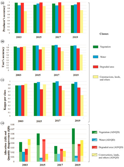
Figure 5.
Level 1 accuracy statistics: (a) Producer’s and; (b) user’s accuracy per class for 2003, 2015, 2017, and 2019 imagery; (c) Kappa per class index (Level 1 of classification); (d) allocation and quantity disagreements.
3.1.2. Mangrove Species (Level 3) Classification
In general, level 3 classification accuracies are above 0.80. For the years 2003, 2015, 2017, and 2019, Avicennia class producer’s accuracies are 0.77, 0.93, 0.93, and 0.82, respectively, while Rhizophora class accuracies are 0.94, 0.85, 0.91, and 0.95 (Figure 6a). However, user’s accuracies for years 2003, 2015, 2017, and 2019 in the Avicennia class are 0.90, 0.80, 0.87, and 0.91, and in the Rhizophora class are 0.83, 0.94, 0.95, and 0.87, respectively (Figure 6b). Kappa overall indices are above 0.70, and Kappa per class indices oscillate between 0.60 and 0.80 (Figure 6c). Although the Kappa values have been low for some years, these are consistent with similar studies that classify mangrove species, e.g., [45,53,54]. In general, AD presents higher values than QD (Figure 6d), excluding 2003, where QD (0.07) in Rhizophora and Avicennia classes was higher than AD (0.06).
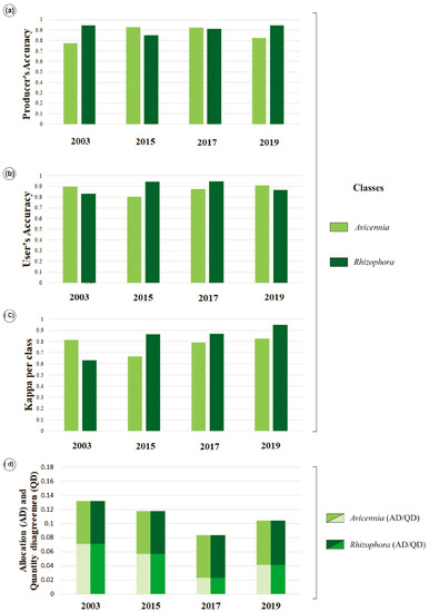
Figure 6.
Level 3 accuracy statistics: (a) Producer’s and; (b) user’s accuracy per class for 2003, 2015, 2017, and 2019 imagery; (c) Kappa index); (d) allocation and quantity disagreements.
3.2. Mid and High-Resolution Vegetation Mapping
The mid-resolution dataset mapping revealed that degraded mangrove area decreased (Figure 6) from 429 in 1986 to 181 ha in 2019 due to natural mangrove recolonization (Table 3). Degraded area dynamics are summarized in Figure 7 and Figure 8. The general trend is a reduction in total degraded area, with two incremental pulses between 1993 and 1999 (+37.92 ha) and 2010 and 2015 (+11.30 ha), wherein the degraded area increased. The high-resolution dataset also shows an increase in the degraded area between 2015 and 2017 (+47.46 ha).
Table 3.
Mangrove degraded areas from 1986 to 2019 using mid and high-resolution datasets.
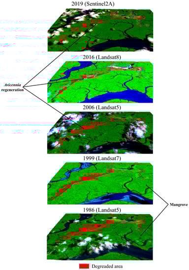
Figure 7.
Spatial-temporal changes of the degraded mangrove area using mid-resolution imagery from 1986 to 2019.
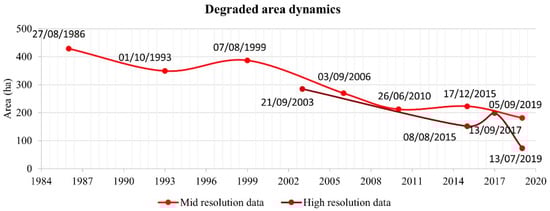
Figure 8.
Degraded mangrove areas using mid and high-resolution images between 1986 and 2019.
Differences in the mid and high-resolution degraded areas, for instance in 2015, may be attributed to the mid-resolution sensors of the Landsat that tend to unify the spectral response of various objects (mangrove shrubs, roads, the floodplain) in one pixel, while the high-resolution dataset allows identifying precisely, for instance, mangrove shrubs and seedlings.
The high-resolution dataset indicates stable mangrove forests covering ~4280 ha (46% of the study area) (Figure 9). Between 2003 and 2019, mangrove gain was ~1328 ha, spatially concentrated in the degraded area and on a tidal bar southeast of the study area. Mangrove retreat was ~637 ha, mainly characterized by the erosion of the Taperaçu channel and Caeté estuary. The remaining degraded mangrove area was ~72.9 ha in 2019 (Figure 9). The degraded area occupied 284 ha in 2003, and only 151 ha in 2015 (Figure 10). This trend was caused by the Avicennia recolonization along the borders and in the middle of the degraded area. However, the degradation increased to 199 ha in 2017, followed by a strong retraction in 2019 to 72.9 ha (Figure 10). In 2019, a mangrove succession started, with Rhizophora colonizing areas previously occupied by Avicennia.
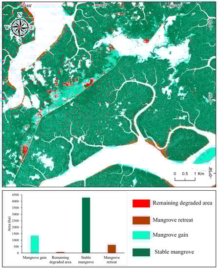
Figure 9.
Spatial distribution of landcover changes based on the high-resolution dataset between 2003 and 2019.
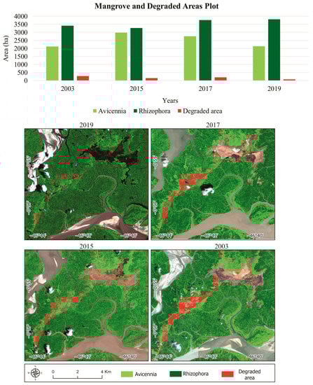
Figure 10.
Graphs showing changes in areas dominated by Avicennia, Rhizophora, and degraded mangroves associated with the spatial-temporal changes of the mangrove cover in the Bragança Peninsula using high-resolution images from 2013 to 2019.
Therefore, a significant contraction in the degraded area from 284.60 to 72.90 ha occurred between 2003 and 2019 due to the recolonization of Avicennia (72 ha), Rhizophora (55 ha), and incipient mangrove (85.70 ha) (Figure 11). In this time interval (16 years), 74.5% of the degraded area was regenerated mainly by Avicennia trees and incipient mangroves. The low tree stature and dispersion of incipient mangrove recolonization hampered a clear identification of the mangrove genus. However, considering the Avicennia trees are the pioneers in the recolonization of the degraded area, the incipient mangrove area is likely comprised mostly of the seedlings of Avicennia.
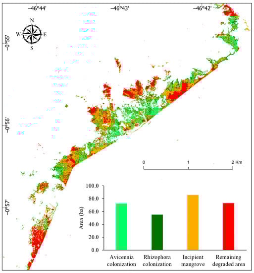
Figure 11.
Changes in the mangrove degraded area between 2003 and 2019 using high-resolution images.
3.3. Vegetation Height and Topographic Analysis
Three-dimensional models (DSM, DTM, and DVHM) and longitudinal sections revealed the topographic features of the degraded area in the Bragança Peninsula. Highway PA-458 marks a threshold between two different vegetation height regions. On the SE side of the road, the vegetation height oscillates between 10 and 25 m, while on the NW side, where there are mangroves, vegetation heights are <10 m (Figure 12a). The topographically higher flats occur on the SE side of the road (Figure 12b), which could be related to higher sedimentation input from the Caeté estuary, due to the damming of tidal channels near the road. Depressions close to the road are typically characterized by flooded zones on the NW side (Figure 12b), as a result of the interruption of the drainage network.
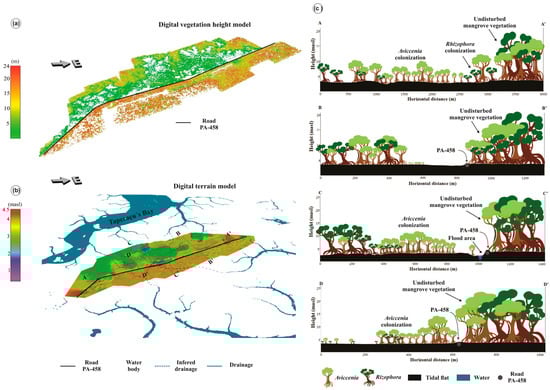
Figure 12.
Digital Models for (a) vegetation height and (b) terrain. (c) Planialtimetric sections (A-A’, B-B’, C-C’ and D-D’) of the degraded mangrove areas near the center of the Bragança Peninsula related to mean sea level with the vegetation units and vegetation height.
Despite the mangrove regeneration in the peninsula, the remnants of the degraded area are directly related to the topographically elevated regions (~3.5–3.8 m amsl) on the NW side of the road. Four sections, three transverse (B, C, and D) and one longitudinal (A) to the PA-458 road of the Bragança Peninsula revealed the mangrove regeneration dynamics. The A-A’ section highlights an Avicennia colonization with tree heights of ~6 m at the center side of the degraded area (Figure 12c). Rhizophora trees ~2 m tall are colonizing smaller areas, suggesting that Rhizophora colonization took place after the Avicennia’s trees colonization.
The B-B’ section shows remnants of the degraded area (Figure 12c), characterized by a frequently flooded depression. The C-C’ section (Figure 12c) suggests dammed waters close to the road, producing permanent lakes, and Avicennia regeneration preferentially occurring on periodically flooded flats. The D-D’ section presents the recolonization of tidal flats by Avicennia and some Rhizophora trees with a positive slope toward the road, which produces a typical tidal inundation frequency instead of depression with permanent flooding (Figure 12c).
4. Discussion
4.1. Mid-Resolution Dataset Analysis
The high contrast in the spectral response between degraded areas and mangrove forests allowed us to map the degraded areas in the mid-resolution dataset manually. However, the high temporal resolution of this data contrasts with indistinguishable objects smaller than the pixel size (900 m2). Therefore, the degraded area borders mapping will be restricted by the uncertainties caused by the pixels with mixed coverages (e.g., herbaceous plants, soil, and water). These areas will have a spectral response resulting from an average reflectance between the different types of coverage that the pixel contains [55].
The mid-resolution dataset’s spatial-temporal analysis (1986–2019) indicated a decreasing trend in the degraded area due to mangrove recolonization. Cohen and Lara [31] recorded this mangrove recolonization in the 1990s. Although our study indicates a pulse of increase in the degraded areas in the 1990s, the overall trend between 2000 and 2019 is a mangrove recolonization (Figure 7). Our analysis also indicated two increased pulses of the degraded area (Figure 8). These pulses seem to be related to extreme weather events, such as strong “El Niño” episodes in 1997–1998 and 2015 with below-average annual rainfall and an exceptionally low or non-existent percentage of clouds (Figure 13). It suggests that dry climatic conditions in the study area favor the degradation of the newly established mangrove due to an increased porewater salinity that harms the Avicennia metabolism, leading them to death, e.g., [56,57].
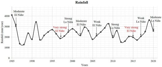
Figure 13.
Annual precipitation values in the Bragança peninsula (mm) with the “El Niño” and “La Niña” phenomena for the analyzed scenes [58,59].
4.2. High-Resolution Dataset Analysis
The accuracy of the high-resolution dataset was satisfactory, but some considerations must be accounted for, especially in the mangrove species classification (Level 3). The degraded area class presented user accuracy below 0.9 in 2015 and 2019, which could be explained by the high presence of clouds in these scenes. Clouds generate changes in the spectral response of the coverages and, therefore, have difficulties in differentiating coverages with classification algorithms. Since the high-resolution imagery was used as reference data, there are uncertainties regarding the reliability of the classification. To mitigate these issues, the GCPs used to validate the 3D models were also used to calculate the accuracy of the 2019 image classification. Another challenge presented by this classification was the lack of acquisition data for the high-resolution imagery (both Pleiades and Google Earth Pro data). To perform the mangrove species separation, we took advantage of the difference in the spectral response that the two species have between the wavelengths of 500 and 600 nm [60]. The wavelength interval in the Pleiades-1 sensor corresponds to the green band. That difference in the green band response was also seen in the 2003 Google Earth Pro image; this classification was much more challenging and presented the lowest accuracy values.
Additionally, the spatial-temporal analysis based on a high-resolution dataset between 2003 and 2019 revealed that the dominating process was the mangrove expansion, overcoming the mangrove retreat. These data indicated the development of Rhizophora on flats previously occupied by Avicennia, likely due to a general reduction in porewater salinity. Comparing the mid and high-resolution data results, both presented the same trend of reduced degraded areas from 2003 to 2019 (Figure 8). However, there is a difference in the quantification of the results (Table 3), which is related to the low capability of the mid-resolution sensors to detect isolated mangrove shrubs or trees, incipient mangrove, and low-density vegetation due to the spatial resolution of the selected images. On the other hand, high-resolution imagery has pixel sizes between 0.5 m and 2 m, which combined with field observations, allowed the identification of the incipient mangrove class (Figure 11). This class corresponds to low-height mangrove sprouts and shrubs.
Multiple source datasets offered the possibility of obtaining two perspectives on degradation/regeneration occurring in Bragança’s mangrove forests. The mid-resolution dataset (Landsat and SAR data) and the methodology for the degraded area estimation did not allow us to accurately-quantify those areas. This dataset permitted us to understand the degradation/regeneration tendency due to the historical availability. The high-resolution dataset, with the spectral, geometric, and texture features, helped to quantify mangrove dynamics. This reliable quantification is evident in the accuracy assessment results of the proposed classes. We did not combine different resolution datasets to avoid classification uncertainties. Hence, both were presented together for comparative purposes. Drone data was restricted to obtain vegetation height and tidal flat topography information.
4.3. Topographic Data Considerations
Regarding drone imagery acquisition, challenges such as the influence of viewing geometry, geometric corrections, shadows, and acquisition time, among others, can reduce the capability to generate detailed quantitative information [61]. The GCPs acquired during fieldwork mostly corrected these error factors. However, 3D cloud manual depuration took great effort to produce digital models more approximated to the actual terrain data in the Bragança Peninsula. Planialtimetric data obtained by photogrammetry combined with topographic data obtained by theodolite survey represented key information to validate the mangrove dynamics in the degraded area.
Morphological features such as depressions served as a tool to interpret small tidal creeks (Figure 12b), which are essential in understanding the hydrodynamics affected by the PA-458 road construction. The cross-sections show how degradation has been more extensive in the zones with tidal channels disconnected from the Caeté estuary (Figure 12b). It is evident in the cross-profile A-A’ (Figure 12c), where mangroves in the SW zone, with several channels cut by the road, showed extensive mangrove degradation. This is in contrast with the NE sector, which had no interruption in the drainage network and thus no significant signs of mangrove degradation, despite being the same distance from the road.
The topographic control over the mangrove development is evident in the B-B’ section (Figure 12c). Mangrove regeneration occurs on surfaces subject to a regular tidal flood regime. Alternately, depressions with tidal channels obstructed by the road tend to accumulate tidal water, leading to mangrove degradation. This degradation may occur in depressions permanently flooded due to porewater sulfides, a phytotoxin in wetlands that accumulates during permanent flooding conditions [62]. Low redox potential (Eh) and high sulfide concentrations are typical of sediments in permanent flooding depressions. Sulfate-reducing bacteria oxidize organic matter in substrates under the marine influence. Low Eh and sulfidic sediment are hostile to mangroves [63].
In addition, depressions tend to accumulate tidal water subject to evaporation mainly during the dry period, causing a significant increase in the porewater salinity. This process causes hypersalinization of tidal flats, hampering mangrove growth and regeneration [25,30]. Increased salinity is a major environmental stress inhibiting plant growth by increasing the levels of toxic ions such as Na+ and Cl− [64,65]. Mangroves have morphological and physiological adaptations to survive under saline conditions [64]. Changes in porewater salinity gradients in time and space control the mangrove distribution [66]. Ball [67] indicated that the salinity gradient controls the maximal mangrove growth. Mangrove species can grow in a wide range of porewater salinity, even in about three times seawater salinity (~90‰) [68]. However, a hypersalination of tidal flats may cause mangrove death or inhibit its growth and development [69,70,71].
Topographic depressions were formed only on the side of the PA-458 road under the influence of the Taperaçu channel, exactly where the degradation of the mangroves occurred (Figure 12). Therefore, the construction of highway PA-458 should have been designed to cross mangrove areas on the highest tidal flats and to skirt the channel headwaters to avoid disrupting regular tidal flow along these channels.
4.4. Effects of Road Construction on Mangrove Dynamics
The construction of the PA-458 road modified the hydrodynamics at the center of the Bragança Peninsula (Figure 11b and Figure 13). The effect of road building on ecosystems includes changes in hydrological factors such as water movement, infiltration patterns, and tidal pumping [72]. Changes in these features result from the interruption of tidal channels that control the porewater salinity and, subsequently, mangrove development [32]. The spatial-temporal analysis shows degradation mainly on the NW side of the road. This degradation is likely related to higher salinity values of the Taperaçu channel and limited sediment and freshwater input from fluvial sources compared to the Caeté estuary (Figure 7) [42]. The NW side of the road experienced increased porewater salinity after the interruption of the regular tidal flood regime with mixtures of the tidal waters of Caeté and Taperaçu in the central area of the peninsula (Figure 14), causing a porewater salinity contrast between the NW (degraded mangrove with >70‰) and SE of the studied area (Avicennia Forest with <50‰) (Figure 3). In addition, the road construction caused depressions and elevations on the NW and SE sides of this road, respectively (Figure 12), due to interruption in the sedimentary dispersion conducted by the tidal channels under the influence of the Caeté estuary. Such depressions with permanent flooding caused mangrove death and prevented mangrove recolonization. Avicennia, which presents high tolerance to high porewater salinity [73,74], recolonized mainly tidal flats that flooded periodically (Figure 12). That explains the mangrove degradation occurring only on the NW side of the road and how this road interfered with the drainage system and affected the sediment’s physical-chemical characteristics.
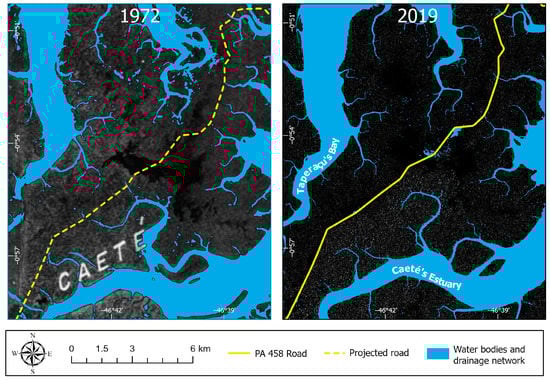
Figure 14.
Radar imagery showing the drainage network before (1972, X-band, Side-Looking Airborne Radar) and after (2019, Sentinel-1 C-band Synthetic Aperture Radar) the construction of Highway PA-458.
The effect of road construction on the environment has been described in other localities, affecting environmental properties such as pH, bulk density, moisture, conductivity, organic matter, etc., causing several changes in vegetation cover, soil properties, and light regimes [75]. The ecological effect of the road includes habitat fragmentation and affecting the flora and fauna populations [76]. In the Bragança Peninsula, this phenomenon, combined with other agents such as reduced precipitation rates, contributed to the rapid degradation of mangrove forests. The sediment input to the mangrove tidal flats has vital importance due to the supply of nutrients [77]. Thus, it represents another negative impact of this road on the studied mangroves, as it cut off the sediment flow from the Caeté estuary to the NW side of the study area (Figure 14). In addition, this road caused a topographical difference in the substrates under the influence of the Caeté (with higher fluvial sediment supply) and Taperaçu. The elevation of the substrate influenced by the Caeté is higher than the flats under the influence of the Taperaçu. The changes in tidal channels from high connectivity to low connectivity caused a reduction in the sediment transport speed [78], which resulted in a lesser amount of suspended sediment to feed the mangroves on the NW side of the road.
Similar studies reveal that the buffer of environmental changes related to road construction is ~1 km, e.g., [79,80]. In the Bragança Peninsula, this buffer reached up to 2 km, but mainly toward the Taperaçu side. The negative ecological impact of Highway PA-458 suggests the importance of accurate design studies for construction in pristine coastal environments. Studies on the relationship between mangrove dynamics, drainage system, topography, and tidal inundation frequency on muddy flats before road construction provide an excellent opportunity to avoid unnecessary adverse road effects on the vegetation cover in terrestrial and aquatic ecosystems, e.g., [75,76]. In this case, Highway PA-458 should have been built in the nearby topographically higher regions, thus avoiding cutting the tidal channels. Furthermore, additional engineering works such as pipes connecting the underground tidal channels should have been considered during the PA-458 construction.
4.5. Climatic Factors and Sea-Level Rise Affecting Mangrove Regeneration
Changes in localized precipitation modified the regeneration rates of the degraded area. Our data indicated that high rainfall increases mangrove regeneration (Figure 7 and Figure 12), due to a decreasing porewater salinity during wet periods. Extreme low and extreme high precipitation are related to the “El Niño” and “La Niña” phenomena. Very strong “El Niño” conditions caused an increase in the degraded area due to the dominance of drier and likely higher pore salinity conditions during 1998 and 2015, years in which the study area was under these conditions. Conversely, strong “La Niña” conditions contributed to the decrease in the degraded area in 2000 and 2010. Although climatic factors appear to be a major factor in altering the regeneration rates, it is not the primary factor controlling mangrove regeneration in this study region.
Historically, relative sea-level rise controlled mangrove dynamics at the Bragança Peninsula [25,30,31,81,82]. During episodes of relative sea-level rise, mangroves migrate to topographically more elevated areas. In contrast, during relative sea-level fall, mangroves migrate seaward, and herbaceous vegetation colonizes more elevated areas in the Bragança Peninsula [25]. Several authors indicated that relative sea-level rise has an active effect on the northern coast of Brazil, e.g., [29,30,41,82]. The global average sea-level rise trend during the last decades (Figure 15), combined with the soft topography of the tidal flat in the Bragança Peninsula, seems to stabilize the hydrological dynamics affected by the PA-458 road construction. Thus, sea-level rise may have triggered the mangrove regeneration by colonizing Avicennia and Rhizophora mangrove trees from the lower to higher flats (Figure 11 and Figure 12). However, permanently flooded depressions are unlikely to be recolonized by mangroves unless connections are re-established between these depressions with drainage on the Caeté estuary through pipes or bridges to prevent water accumulation between the road and these depressions.
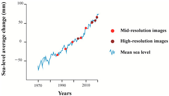
Figure 15.
Mean sea-level fluctuations between 1970 and 2020 with satellite imagery acquisition dates (points) from this study. Modified from Lindsey [83].
5. Conclusions
The construction of Highway PA-458 in 1973 degraded at least 430 ha of mangroves in the Bragança Peninsula. A radar image obtained in 1972 indicated that the road construction interrupted tidal channels previously connected with the Caeté estuary and caused topographic contrasts between both sides of this road, resulting in increased porewater salinity on the NW side. Depressions permanently or semi-permanently inundated also degraded part of the original mangrove forests, preventing mangrove regeneration in some locations of the Bragança Peninsula. However, mid and high-resolution data indicated mangrove recolonization on flats regularly flooded by the tide at rates of 7.51 ha/yr and 13.22 ha/yr between 1986 and 2019 and 2003 and 2019, respectively. Mangrove species mapping of the high-resolution dataset revealed that the recolonization process occurs among both of the two main mangrove species in the Bragança Peninsula (Rhizophora mangle and Avicennia germinans). Rhizophora trees recolonized areas along the lower flats of degraded mangroves, while Avicennia recolonized higher tidal flats of degraded mangroves closer to the highway. Ephemeral control over mangrove degradation/regeneration on the Bragança Peninsula was related to extreme climatic events such as “El Niño” and “La Niña.” In contrast, relative sea-level rise during the last decades may have caused a long-term mangrove recolonization from lower to higher tidal flats, as revealed by the spatial-temporal analysis along topographic profiles. Nevertheless, permanently flooded depressions are unlikely to be recolonized by mangroves unless connections are re-established between these depressions with active drainages on the Caeté estuary through pipes or bridges to prevent permanent or semi-permanent water accumulation between the road and these depressions. To minimize the impacts on mangroves, the Highway PA-458 construction should have been designed to cross mangrove areas on the highest tidal flats and skirt the channel headwaters to avoid interruption of regular tidal flow along these channels.
Author Contributions
Methodology, S.M.M.C., M.C.L.C., A.V.S. and J.S.G.-N.; Validation, S.M.M.C., M.C.L.C., D.P.C.R. and A.V.S.; Formal analysis, S.M.M.C. and M.C.L.C.; Investigation, S.M.M.C., M.C.L.C., D.P.C.R., A.V.S. and L.C.R.P.; Resources, M.C.L.C. and L.C.R.P.; Data curation, S.M.M.C.; Writing—original draft, S.M.M.C.; Writing—review & editing, S.M.M.C., M.C.L.C., D.P.C.R., A.V.S., J.S.G.-N., L.C.R.P. and N.C.; Visualization, M.C.L.C. and J.S.G.-N.; Project administration, M.C.L.C.; Funding acquisition, M.C.L.C. All authors have read and agreed to the published version of the manuscript.
Funding
This research was funded by National Council for Scientific and Technological Development, grant number 403239/2021-4; São Paulo Research Foundation, grant number 2020/13715-1.
Data Availability Statement
Data is available upon request.
Acknowledgments
We want to thank the Laboratory of Coastal Dynamic (LADIC-UFPA) and the Geotechnologies teaching and research laboratory (LEPGEO-UFPA) for their support. The imagery used in this research was sponsored by the “NoR Sponsorship program” from the European Space Agency.
Conflicts of Interest
The authors declare no conflict of interest.
References
- Woodroffe, C.D.; Grindrod, J. Mangrove Biogeography: The Role of Quaternary Environmental and Sea-Level Change. J. Biogeogr. 1991, 18, 479–492. [Google Scholar] [CrossRef]
- Woodroffe, C.D. Response of Tide-dominated Mangrove Shorelines in Northern Australia to Anticipated Sea-Level Rise. Earth Surf. Process. Landf. 1995, 20, 65–85. [Google Scholar] [CrossRef]
- Spalding, M.; Kainuma, M.; Collins, L. World Atlas of Mangroves; Earthscan: London, UK, 2010; ISBN 9781844076574. [Google Scholar]
- Giri, C.; Ochieng, E.; Tieszen, L.L.; Zhu, Z.; Singh, A.; Loveland, T.; Masek, J.; Duke, N. Status and Distribution of Mangrove Forests of the World Using Earth Observation Satellite Data. Glob. Ecol. Biogeogr. 2011, 20, 154–159. [Google Scholar] [CrossRef]
- Twilley, R.R.; Day, J.W. Mangrove Wetlands. In Estuarine Ecology, 2nd ed.; Day, J.W., Jr., Kemp, W.M., Yáñez-Arancibia, A., Crump, B.C., Eds.; John Wiley & Sons: Hoboken, NJ, USA, 2012; pp. 165–202. ISBN 9780471755678. [Google Scholar]
- Mitsch, W.J.; Gosselink, J.G. Wetlands, 4th ed.; John Wiley and Sons: Hoboken, NJ, USA, 2007; ISBN 978-0-471-69967-5. [Google Scholar]
- Food and Agriculture Organization (FAO). The World’s Mangroves 1980–2005. A Thematic Study Prepared in the Framework of the Global Forest Resources Assessment 2005; FAO: Rome, Italy, 2007; ISBN 978-92-5-105856-5.
- Mitsch, W.J.; Mander, Ü. Wetlands and Carbon Revisited. Ecol. Eng. 2018, 114, 1–6. [Google Scholar] [CrossRef]
- Soper, F.M.; MacKenzie, R.A.; Sharma, S.; Cole, T.G.; Litton, C.M.; Sparks, J.P. Non-Native Mangroves Support Carbon Storage, Sediment Carbon Burial, and Accretion of Coastal Ecosystems. Glob. Chang. Biol. 2019, 25, 4315–4326. [Google Scholar] [CrossRef]
- Doyle, T.W.; Girod, G.F.; Books, M.A. Modeling Mangrove Forest Migration along the Southwest Coast of Florida under Climate Change. In Integrated Assessment of the Climate Change Impacts on the Gulf Coast Region; Ning, Z., Turner, R.E., Doyle, T.W., Abdollahi, K., Thornton, A., Reyes, E., Justic, D., Swenson, E., Khairy, W., Liu, K., Eds.; GCRCC: Baton Rouge, LA, USA, 2003; pp. 211–222. [Google Scholar]
- Kirwan, M.L.; Murray, A.B. A Coupled Geomorphic and Ecological Model of Tidal Marsh Evolution. Proc. Natl. Acad. Sci. USA 2007, 104, 6118–6122. [Google Scholar] [CrossRef]
- Cohen, M.C.L.; Pessenda, L.C.R.; Behling, H.; de Fátima Rossetti, D.; França, M.C.; Guimarães, J.T.F.; Friaes, Y.; Smith, C.B. Holocene Palaeoenvironmental History of the Amazonian Mangrove Belt. Quat. Sci. Rev. 2012, 55, 50–58. [Google Scholar] [CrossRef]
- Hamilton, S.E.; Casey, D. Creation of a High Spatio-Temporal Resolution Global Database of Continuous Mangrove Forest Cover for the 21st Century (CGMFC-21). Glob. Ecol. Biogeogr. 2016, 25, 729–738. [Google Scholar] [CrossRef]
- Thomas, N.; Lucas, R.; Bunting, P.; Hardy, A.; Rosenqvist, A.; Simard, M. Distribution and Drivers of Global Mangrove Forest Change, 1996–2010. PLoS ONE 2017, 12, e0179302. [Google Scholar] [CrossRef]
- Beselly, S.M.; van der Wegen, M.; Grueters, U.; Reyns, J.; Dijkstra, J.; Roelvink, D. Eleven Years of Mangrove–Mudflat Dynamics on the Mud Volcano-Induced Prograding Delta in East Java, Indonesia: Integrating Uav and Satellite Imagery. Remote Sens. 2021, 13, 1084. [Google Scholar] [CrossRef]
- Hsu, A.J.; Kumagai, J.; Favoretto, F.; Dorian, J.; Martinez, B.G.; Aburto-Oropeza, O. Driven by Drones: Improving Mangrove Extent Maps Using High-Resolution Remote Sensing. Remote Sens. 2020, 12, 3986. [Google Scholar] [CrossRef]
- Lucas, R.; Van De Kerchove, R.; Otero, V.; Lagomasino, D.; Fatoyinbo, L.; Omar, H.; Satyanarayana, B.; Dahdouh-Guebas, F. Structural Characterisation of Mangrove Forests Achieved through Combining Multiple Sources of Remote Sensing Data. Remote Sens. Environ. 2020, 237, 111543. [Google Scholar] [CrossRef]
- Xia, J.; Yokoya, N.; Pham, T.D. Probabilistic Mangrove Species Mapping with Multiple-Source Remote-Sensing Datasets Using Label Distribution Learning in Xuan Thuy National Park, Vietnam. Remote Sens. 2020, 12, 3834. [Google Scholar] [CrossRef]
- Sakti, A.D.; Fauzi, A.I.; Wilwatikta, F.N.; Rajagukguk, Y.S.; Sudhana, S.A.; Yayusman, L.F.; Syahid, L.N.; Sritarapipat, T.; Principe, J.A.; Quynh Trang, N.T.; et al. Multi-Source Remote Sensing Data Product Analysis: Investigating Anthropogenic and Naturogenic Impacts on Mangroves in Southeast Asia. Remote Sens. 2020, 12, 2720. [Google Scholar] [CrossRef]
- Younes Cárdenas, N.; Joyce, K.E.; Maier, S.W. Monitoring Mangrove Forests: Are We Taking Full Advantage of Technology? Int. J. Appl. Earth Obs. Geoinf. 2017, 63, 1–14. [Google Scholar] [CrossRef]
- Wang, L.; Sousa, W.P.; Gong, P.; Biging, G.S. Comparison of IKONOS and QuickBird Images for Mapping Mangrove Species on the Caribbean Coast of Panama. Remote Sens. Environ. 2004, 91, 432–440. [Google Scholar] [CrossRef]
- Wan, L.; Zhang, H.; Lin, G.; Lin, H. A Small-Patched Convolutional Neural Network for Mangrove Mapping at Species Level Using High-Resolution Remote-Sensing Image. Ann. GIS 2019, 25, 45–55. [Google Scholar] [CrossRef]
- Cohen, M.C.L.; Figueiredo, B.L.; Oliveira, N.N.; Fontes, N.A.; França, M.C.; Pessenda, L.C.R.; de Souza, A.V.; Macario, K.; Giannini, P.C.F.; Bendassolli, J.A.; et al. Impacts of Holocene and Modern Sea-Level Changes on Estuarine Mangroves from Northeastern Brazil. Earth Surf. Process. Landforms. 2020, 45, 375–392. [Google Scholar] [CrossRef]
- Bozi, B.S.; Figueiredo, B.L.; Rodrigues, E.; Cohen, M.C.L.; Pessenda, L.C.R.; Alves, E.E.N.; de Souza, A.V.; Bendassolli, J.A.; Macario, K.; Azevedo, P.; et al. Impacts of Sea-Level Changes on Mangroves from Southeastern Brazil during the Holocene and Anthropocene Using a Multi-Proxy Approach. Geomorphology 2021, 390, 107860. [Google Scholar] [CrossRef]
- Cohen, M.C.L.; Camargo, P.M.P.; Pessenda, L.C.R.; Lorente, F.L.; De Souza, A.V.; Corrêa, J.A.M.; Bendassolli, J.; Dietz, M. Effects of the Middle Holocene High Sea-Level Stand and Climate on Amazonian Mangroves. J. Quat. Sci. 2021, 36, 1013–1027. [Google Scholar] [CrossRef]
- Cohen, M.C.L.; Rodrigues, E.; Rocha, D.O.S.; Freitas, J.; Fontes, N.A.; Pessenda, L.C.R.; de Souza, A.V.; Gomes, V.L.P.; França, M.C.; Bonotto, D.M.; et al. Southward Migration of the Austral Limit of Mangroves in South America. Catena 2020, 195, 104775. [Google Scholar] [CrossRef]
- Otero, V.; Van De Kerchove, R.; Satyanarayana, B.; Martínez-Espinosa, C.; Fisol, M.A.B.; Ibrahim, M.R.B.; Sulong, I.; Mohd-Lokman, H.; Lucas, R.; Dahdouh-Guebas, F. Managing Mangrove Forests from the Sky: Forest Inventory Using Field Data and Unmanned Aerial Vehicle (UAV) Imagery in the Matang Mangrove Forest Reserve, Peninsular Malaysia. For. Ecol. Manag. 2018, 411, 35–45. [Google Scholar] [CrossRef]
- Souza-Filho, P.W.M.; Paradella, W.R. Use of RS1 Fine Mode and Landsat-5 TM PCA for Geomorphological Mapping in a Microtidal Mangrove Coast in the Amazon Region. Can. J. Remote. Sens. 2005, 31, 214–224. [Google Scholar] [CrossRef]
- Nascimento, W.R.; Souza-Filho, P.W.M.; Proisy, C.; Lucas, R.M.; Rosenqvist, A. Mapping Changes in the Largest Continuous Amazonian Mangrove Belt Using Object-Based Classification of Multisensor Satellite Imagery. Estuar. Coast. Shelf Sci. 2013, 117, 83–93. [Google Scholar] [CrossRef]
- Cohen, M.C.L.; de Souza, A.V.; Rossetti, D.F.; Pessenda, L.C.R.; França, M.C. Decadal-Scale Dynamics of an Amazonian Mangrove Caused by Climate and Sea Level Changes: Inferences from Spatial–Temporal Analysis and Digital Elevation Models. Earth Surf. Process. Landfo 2018, 43, 2876–2888. [Google Scholar] [CrossRef]
- Cohen, M.C.L.; Lara, R.J. Temporal Changes of Mangrove Vegetation Boundaries in Amazonia: Application of GIS and Remote Sensing Techniques. Wetl. Ecol. Manag. 2003, 11, 223–231. [Google Scholar] [CrossRef]
- Lara, R.J.; Cohen, M.C.L. Sediment Porewater Salinity, Inundation Frequency and Mangrove Vegetation Height in Bragança, North Brazil: An Ecohydrology-Based Empirical Model. Wetl. Ecol. Manag. 2006, 14, 349–358. [Google Scholar] [CrossRef]
- Cunha-Lignon, M.; Menghini, R.P.; Santos, L.C.M.; Niemeyer-Dinóla, C.; Schaeffer-Novelli, Y. Estudos de Caso Nos Manguezais Do Estado de São Paulo (Brasil): Aplicação de Ferramentas Com Diferentes Escalas Espaço-Temporais. Rev. Gestão Costeira Integr. 2009, 9, 79–91. [Google Scholar] [CrossRef]
- Villate Daza, D.A.; Moreno, H.S.; Portz, L.; Manzolli, R.P.; Bolívar-Anillo, H.J.; Anfuso, G. Mangrove Forests Evolution and Threats in the Caribbean Sea of Colombia. Water 2020, 12, 1113. [Google Scholar] [CrossRef]
- Patel, B.K.; Vachrajani, K.D. Pollution Status in Mangrove Ecosystem of Mahi and Dadhar River Estuaries. In National Conference on Biodiversity: Status and Challenges in Conservation—‘FAVEO’; 2013; pp. 163–172. Available online: http://www.vpmthane.org/sci/faveo/r27.pdf (accessed on 27 September 2022).
- Din, N.; Ngo-Massou, V.M.; Essomè-Koum, G.L.; Ndema-Nsombo, E.; Kottè-Mapoko, E.; Nyamsi-Moussian, L. Impact of Urbanization on the Evolution of Mangrove Ecosystems in the Wouri River Estuary (Douala Cameroon). In Coastal Wetlands: Alteration and Remediation; Finkl, C.W., Makowski, C., Eds.; Springer International Publishing: Cham, Swizerland, 2017; Volume 21, pp. 81–131. ISBN 978-3-319-56179-0. [Google Scholar]
- Fernandes, M.E.B.; Fernandes, J.S.; Muriel-Cunha, J.; Sedovim, W.R.; Gomes, I.A.; Santana, D.S.; Sampaio, D.S.; Andrade, F.A.G.; Oliveira, F.P.; Brabo, L.B.; et al. Efeito Da Construção Da Rodovia PA-458 Sobre as Florestas de Mangue da Península Bragantina, Bragança, Pará, Brasil. UAKARI 2007, 3, 55–63. [Google Scholar] [CrossRef][Green Version]
- Oliveira, M.V.C.; Henrique, M.C. No Meio Do Caminho Havia Um Mangue: Impactos Socioambientais da Estrada Bragança-Ajuruteua, Pará. História, Ciências, Saúde-Manguinhos 2018, 25, 497–514. [Google Scholar] [CrossRef] [PubMed]
- Lara, R.; Szlafsztein, C.; Cohen, M.C.L.; Berger, U.; Glaser, M. Implications of Mangrove Dynamics for Private Land Use in Bragança, North Brazil: A Case Study. J. Coast. Conserv. 2002, 8, 97–102. [Google Scholar] [CrossRef]
- Souza Filho, P.W.M.; Paradella, W.R. Recognition of the Main Geobotanical Features along the Bragança Mangrove Coast (Brazilian Amazon Region) from Landsat TM and RADARSAT-1 Data. Wetl. Ecol. Manag. 2002, 10, 123–132. [Google Scholar] [CrossRef]
- Cohen, M.C.L.; Behling, H.; Lara, R.J.; Smith, C.B.; Matos, H.R.S.; Vedel, V. Impact of Sea-Level and Climatic Changes on the Amazon Coastal Wetlands during the Late Holocene. Veg. Hist. Archaeobot. 2009, 18, 425–439. [Google Scholar] [CrossRef]
- Asp, N.E.; Schettini, C.A.F.; Siegle, E.; da Silva, M.S.; de Brito, R.N.R. The Dynamics of a Frictionally-Dominated Amazonian Estuary. Braz. J. Oceanogr. 2012, 60, 391–403. [Google Scholar] [CrossRef]
- Asp, N.E.; Amorim de Freitas, P.T.; Gomes, V.J.C.; Gomes, J.D. Hydrodynamic Overview and Seasonal Variation of Estuaries at the Eastern Sector of the Amazonian Coast. J. Coast. Res. 2013, 165, 1092–1097. [Google Scholar] [CrossRef]
- Da Cruz, C.C.; Mendoza, U.N.; Queiroz, J.B.; Berrêdo, J.F.; Da Costa Neto, S.V.; Lara, R.J. Distribution of Mangrove Vegetation along Inundation, Phosphorus, and Salinity Gradients on the Bragança Peninsula in Northern Brazil. Plant Soil 2013, 370, 393–406. [Google Scholar] [CrossRef]
- Wang, D.; Wan, B.; Qiu, P.; Su, Y.; Guo, Q.; Wu, X. Artificial Mangrove Species Mapping Using Pléiades-1: An Evaluation of Pixel-Based and Object-Based Classifications with Selected Machine Learning Algorithms. Remote Sens. 2018, 10, 294. [Google Scholar] [CrossRef]
- Heumann, B.W. An Object-Based Classification of Mangroves Using a Hybrid Decision Tree-Support Vector Machine Approach. Remote Sens. 2011, 3, 2440–2460. [Google Scholar] [CrossRef]
- Heenkenda, M.K.; Joyce, K.E.; Maier, S.W.; Bartolo, R. Mangrove Species Identification: Comparing WorldView-2 with Aerial Photographs. Remote Sens. 2014, 6, 6064–6088. [Google Scholar] [CrossRef]
- Hu, Q.; Wu, W.; Xia, T.; Yu, Q.; Yang, P.; Li, Z.; Song, Q. Exploring the Use of Google Earth Imagery and Object-Based Methods in Land Use/Cover Mapping. Remote Sens. 2013, 5, 6026–6042. [Google Scholar] [CrossRef]
- Ye, S.; Pontius, R.G.; Rakshit, R. A Review of Accuracy Assessment for Object-Based Image Analysis: From per-Pixel to per-Polygon Approaches. ISPRS J. Photogramm. Remote Sens. 2018, 141, 137–147. [Google Scholar] [CrossRef]
- ESRI Create Accuracy Assessment Points (Image Analyst). Available online: https://pro.arcgis.com/en/pro-app/latest/tool-reference/image-analyst/create-accuracy-assessment-points.htm (accessed on 8 November 2021).
- Congalton, R.G.; Green, K. Assessing the Accuracy of Remotely Sensed Data: Principles and Practices, 3rd ed.; CRC Press: Boca Raton, FL, USA, 2019; ISBN 9780429052729. [Google Scholar]
- Pontius, R.G.; Millones, M. Death to Kappa: Birth of Quantity Disagreement and Allocation Disagreement for Accuracy Assessment. Int. J. Remote Sens. 2011, 32, 4407–4429. [Google Scholar] [CrossRef]
- Kongwongjan, J.; Suwanprasit, C.; Thongchumnum, P. Comparison of Vegetation Indices for Mangrove Mapping Using THEOS Data. Proc. Asia-Pac. Adv. Netw. 2012, 33, 56–64. [Google Scholar] [CrossRef]
- Zulfa, A.W.; Norizah, K.; Hamdan, O.; Faridah-Hanum, I.; Rhyma, P.P.; Fitrianto, A. Spectral Signature Analysis to Determine Mangrove Species Delineation Structured by Anthropogenic Effects. Ecol. Indic. 2021, 130, 108148. [Google Scholar] [CrossRef]
- Pop, A.; Zoran, M.; Braescu, C.L.; Necsoiu, M.; Serban, F.; Petrica, A. Spectral Reflectance Signification in Satellite Imagery. In Photon Transport in Highly Scattering Tissue, Proceedings of the International Symposium on Biomedical Optics Europe ‘94, Lille, France, 6–10 September 1994; SPIE: Bellingham, WA, USA, 1995; Volume 2326, pp. 436–447. [Google Scholar] [CrossRef]
- Mafi-Gholami, D.; Mahmoudi, B.; Zenner, E.K. An Analysis of the Relationship between Drought Events and Mangrove Changes Along the Northern Coasts of the Persian Gulf and Oman Sea. Estuar. Coast. Shelf Sci. 2017, 199, 141–151. [Google Scholar] [CrossRef]
- Carugati, L.; Gatto, B.; Rastelli, E.; Lo Martire, M.; Coral, C.; Greco, S.; Danovaro, R. Impact of Mangrove Forests Degradation on Biodiversity and Ecosystem Functioning. Sci. Rep. 2018, 8, 13298. [Google Scholar] [CrossRef] [PubMed]
- Instituto Nacional de Meteorologia INMET. Available online: https://portal.inmet.gov.br/ (accessed on 20 June 2021).
- Golden Gate Weather Services GGWS. Available online: http://ggweather.com/enso/oni.htm (accessed on 15 June 2021).
- Rebelo-Mochel, F.; Ponzoni, F.J. Spectral Characterization of Mangrove Leaves in the Brazilian Amazonian Coast: Turiaçu Bay, Maranhão State. An. Acad. Bras. Cienc. 2007, 79, 683–692. [Google Scholar] [CrossRef] [PubMed]
- Kelcey, J.; Lucieer, A. Sensor Correction of a 6-Band Multispectral Imaging Sensor for UAV Remote Sensing. Remote Sens. 2012, 4, 1462–1493. [Google Scholar] [CrossRef]
- Lamers, L.P.M.; Govers, L.L.; Janssen, I.C.J.M.; Geurts, J.J.M.; Van der Welle, M.E.W.; Van Katwijk, M.M.; Van der Heid, T.; Roelofs, J.G.M.; Smolders, A.J.P. Sulfide as a Soil Phytotoxin-a Review. Front. Plant Sci. 2013, 4, 268. [Google Scholar] [CrossRef]
- Holguin, G.; Vazquez, P.; Bashan, Y. The Role of Sediment Microorganisms in the Productivity, Conservation, and Rehabilitation of Mangrove Ecosystems: An Overview. Biol. Fertil. Soils 2001, 33, 265–278. [Google Scholar] [CrossRef]
- Flowers, T.J.; Colmer, T.D. Salinity Tolerance in Halophytes. New Phytol. 2008, 179, 945–963. [Google Scholar] [CrossRef] [PubMed]
- Munns, R.; Tester, M. Mechanisms of salinity tolerance. Annu. Rev. Plant Biol. 2008, 59, 651–681. [Google Scholar] [CrossRef] [PubMed]
- Nguyen, H.T.; Stanton, D.E.; Schmitz, N.; Farquhar, G.D.; Ball, M.C. Growth Responses of the Mangrove Avicennia Marina to Salinity: Development and Function of Shoot Hydraulic Systems Require Saline Conditions. Ann. Bot. 2015, 115, 397–407. [Google Scholar] [CrossRef]
- Ball, M.C. Salinity Tolerance in the Mangroves Aegiceras Corniculatum and Avicennia Marina. I. Water Use in Relation to Growth, Carbon Partitioning, and Salt Balance. Aust. J. Plant Physiol. 1988, 15, 447–464. [Google Scholar] [CrossRef]
- Zhao, X.; Rivera-Monroy, V.H.; Wang, H.; Xue, Z.G.; Tsai, C.F.; Willson, C.S.; Castañeda-Moya, E.; Twilley, R.R. Modeling Soil Porewater Salinity in Mangrove Forests (Everglades, Florida, USA) Impacted by Hydrological Restoration and a Warming Climate. Ecol. Modell. 2020, 436, 109292. [Google Scholar] [CrossRef]
- Krauss, K.W.; Lovelock, C.E.; McKee, K.L.; López-Hoffman, L.; Ewe, S.M.L.; Sousa, W.P. Environmental Drivers in Mangrove Establishment and Early Development: A Review. Aquat. Bot. 2008, 89, 105–127. [Google Scholar] [CrossRef]
- Parida, A.K.; Jha, B. Salt Tolerance Mechanisms in Mangroves: A Review. Trees-Struct. Funct. 2010, 24, 199–217. [Google Scholar] [CrossRef]
- Albuquerque, A.G.B.M.; Ferreira, T.O.; Cabral, R.L.; Nóbrega, G.N.; Romero, R.E.; Meireles, A.J.D.A.; Otero, X.L. Hypersaline Tidal Flats (Apicum Ecosystems): The Weak Link in the Tropical Wetlands Chain. Environ. Rev. 2014, 22, 99–109. [Google Scholar] [CrossRef]
- Coffin, A.W.; Ouren, D.S.; Bettez, N.D.; Borda-de-Água, L.; Daniels, A.E.; Grilo, C.; Jaeger, J.A.G.; Navarro, L.M.; Preisler, H.K.; Rauschert, E.S.J. The Ecology of Rural Roads: Effects, Management and Research. Issues Ecol. 2021, 1–35. [Google Scholar]
- Sherman, R.E.; Fahey, T.J.; Martinez, P. Spatial Patterns of Biomass and Aboveground Net Primary Productivity in a Mangrove Ecosystem in the Dominican Republic. Ecosystems 2003, 6, 384–398. [Google Scholar] [CrossRef]
- Madrid, E.N.; Armitage, A.R.; Lopez-Portillo, J. Avicennia Germinans (Black Mangrove) Vessel Architecture Is Linked to Chilling and Salinity Tolerance in the Gulf of Mexico. Front. Plant Sci. 2014, 5, 503. [Google Scholar] [CrossRef]
- Deljouei, A.; Sadeghi, S.M.M.; Abdi, E.; Bernhardt-Römermann, M.; Pascoe, E.L.; Marcantonio, M. The Impact of Road Disturbance on Vegetation and Soil Properties in a Beech Stand, Hyrcanian Forest. Eur. J. For. Res. 2018, 137, 759–770. [Google Scholar] [CrossRef]
- Trombulak, S.C.; Frissell, C.A. Review of Ecological Effects of Roads on Terrestrial and Aquatic Communities. Conserv. Biol. 2000, 14, 18–30. [Google Scholar] [CrossRef]
- Anthony, E.; Goichot, M. Sediment Flow in the Context of Mangrove Restoration and Conservation; World Wide Fund for Nature: Gland, Switzerland, 2020; ISBN 288085-0968. Available online: http://www.mangrovealliance.org/wp-content/uploads/2020/01/WWF-MCR-Sediment-Flow-in-the-Context-of-Mangrove-Restoration-and-Conservation-v6.5-WEB.pdf (accessed on 27 September 2022).
- McLachlan, R.L.; Ogston, A.S.; Asp, N.E.; Fricke, A.T.; Nittrouer, C.A.; Gomes, V.J.C. Impacts of Tidal-Channel Connectivity on Transport Asymmetry and Sediment Exchange with Mangrove Forests. Estuar. Coast. Shelf Sci. 2020, 233, 106524. [Google Scholar] [CrossRef]
- Liu, S.L.; Liu, Q.; Wang, C.; Yang, J.J.; Deng, L. Effects of road construction on regional vegetation types. J. Appl. Ecol. 2013, 24, 1192–1198. [Google Scholar]
- Feng, S.; Liu, S.; Jing, L.; Zhu, Y.; Yan, W.; Jiang, B.; Liu, M.; Lu, W.; Ning, Y.; Wang, Z.; et al. Quantification of the Environmental Impacts of Highway Construction Using Remote Sensing Approach. Remote Sens. 2021, 13, 1340. [Google Scholar] [CrossRef]
- Cohen, M.C.L.; Souza Filho, P.W.M.; Lara, R.J.; Behling, H.; Angulo, R.J. A Model of Holocene Mangrove Development and Relative Sea-Level Changes on the Bragança Peninsula (Northern Brazil). Wetl. Ecol. Manag. 2005, 13, 433–443. [Google Scholar] [CrossRef]
- Souza-Filho, P.W.M.; Lessa, G.C.; Cohen, M.C.L.; Costa, F.R.; Lara, R.J. The Subsiding Macrotidal Barrier Estuarine System of the Eastern Amazon Coast, Northern Brazil. In Geology of Brazilian Coastal Barriers; Dillenburg, S.F., Hesp, P.A., Eds.; Springer: New York, NY, USA, 2009. [Google Scholar] [CrossRef]
- Lindsey, R. Climate Change: Global Sea Level. Available online: https://www.climate.gov/news-features/understanding-climate/climate-change-global-sea-level (accessed on 1 November 2021).
Publisher’s Note: MDPI stays neutral with regard to jurisdictional claims in published maps and institutional affiliations. |
© 2022 by the authors. Licensee MDPI, Basel, Switzerland. This article is an open access article distributed under the terms and conditions of the Creative Commons Attribution (CC BY) license (https://creativecommons.org/licenses/by/4.0/).