Dynamic Evolution Modeling of a Lake-Terminating Glacier in the Western Himalayas Using a Two-Dimensional Higher-Order Flowline Model

Abstract

To better understand the future evolution of Jiemayangzong Glacier (JMYZG), the headstream of the Yarlung Zangbo River, we simulated its future ice thickness evolution using a two-dimensional higher-order numerical flowline model. Due to the sparsity of in situ observational data, we used a combination of field observations and inversion models of velocity and ice thickness to initialize the model parameters. We validated the parametrizations of the calving scheme by comparing the modeled and observed glacier terminus retreats. To estimate the response of JMYZG to climate change, the ice flow model was forced with different climate scenarios. We found that the JMYZG will retreat under different climate scenarios. By 2100, the volume loss of JMYZG will be approximately 34%, 67% and 81% under SSP1-2.6, SSP3-7.0 and SSP5-8.5, respectively.

1. Introduction

As one of the important components of the cryosphere, mountain glaciers are very sensitive to climate and are often used as indicators to reflect climate change [1,2,3]. It can be known from the Intergovernmental Panel on Climate Change (IPCC) Sixth Annual Report [4] (AR6) that, by 2100, under different climatic scenarios, glaciers will lose mass continuously in general [5]. The retreat of mountain glaciers will have an important impact on global mean sea level (GMSL) changes and water resources [6] and will affect socio-economic development [7,8]. The High Mountains of Asia (HMAs) have the largest glacier reservoir outside of the polar regions [9]. It is thus critical to understand the future changes of glaciers in the HMAs.

Over the past two decades, both the number and area of proglacial lakes have largely increased in the HMAs, particularly in the Himalayan regions [10,11,12,13]. About 10% of the Himalayan glacier population is in direct contact with the proglacial lakes. The formation of proglacial lakes promotes the mass loss of their host glaciers through calving and subaqueous melting. In contrast to land-terminating glaciers, the lake-terminating glaciers have more negative mass loss [14,15], accounting for 32% of the mass loss in the Himalayas. Large-scale and localized studies of Himalayan glacier flow speeds show that the along-flowline surface velocities of lake-terminating glaciers are more than double those of land-terminating glaciers [16,17,18,19]. The force balance change at the glacier terminus likely causes the speed-up of lake-terminating glaciers [16,19,20]. A few studies analyzed the flow regime of lake-terminating glaciers through diagnostic modeling [16,19]. However, no prognostic simulations have been performed of lake-terminating glaciers in the Himalayan regions due mainly to the scarcity of in situ measurements. Meanwhile, the current large-scale glacier evolution models neglect the lake-terminating glacier dynamics, which likely underestimate the future glacier mass loss in the HMAs, particularly in the Himalayas [21,22,23]. Additionally, to save computational resources, large-scale glacier models [22,24] lack a reliable ice dynamics component, which undoubtedly adds uncertainty to the glacier evolution results. Yarlung Zangbo River is an important international river [25], as it provides abundant fresh water resources downstream and is of global importance [26]. As the headstream of Yarlung Zangbo River, Jiemayangzong Glacier (JMYZG) directly affects the change of the local socioeconomic and ecological roles in western Tibet and also the downstream regions [27].

In this study, we used a two-dimensional (2D) higher-order flowline model Polythermal Land Ice Model (PoLIM) [28] combined with remote sensing datasets to simulate the dynamic evolution of JMYZG, a lake-terminating glacier in the western Himalaya. The glacier thickness and surface velocities were relatively well surveyed through ground-penetrating radar (GPR) and the global positioning system (GPS). The main aim of this study is to investigate the dynamic features of JMYZG and predict its future evolution under different climate scenarios. This may have implications for remote-sensing investigations of lake-terminating glaciers and large-scale glacier evolution model developments. The paper is structured as follows. We first briefly introduce JMYZG in Section 2. Next, we introduce the data and methods used in our simulations in Section 3. Then, we present our model results in Section 4 and discuss the historical and future evolution of JMYZG, as well as the sensitivity of the surface mass balance in Section 5. Finally, we draw our conclusions in Section 6.

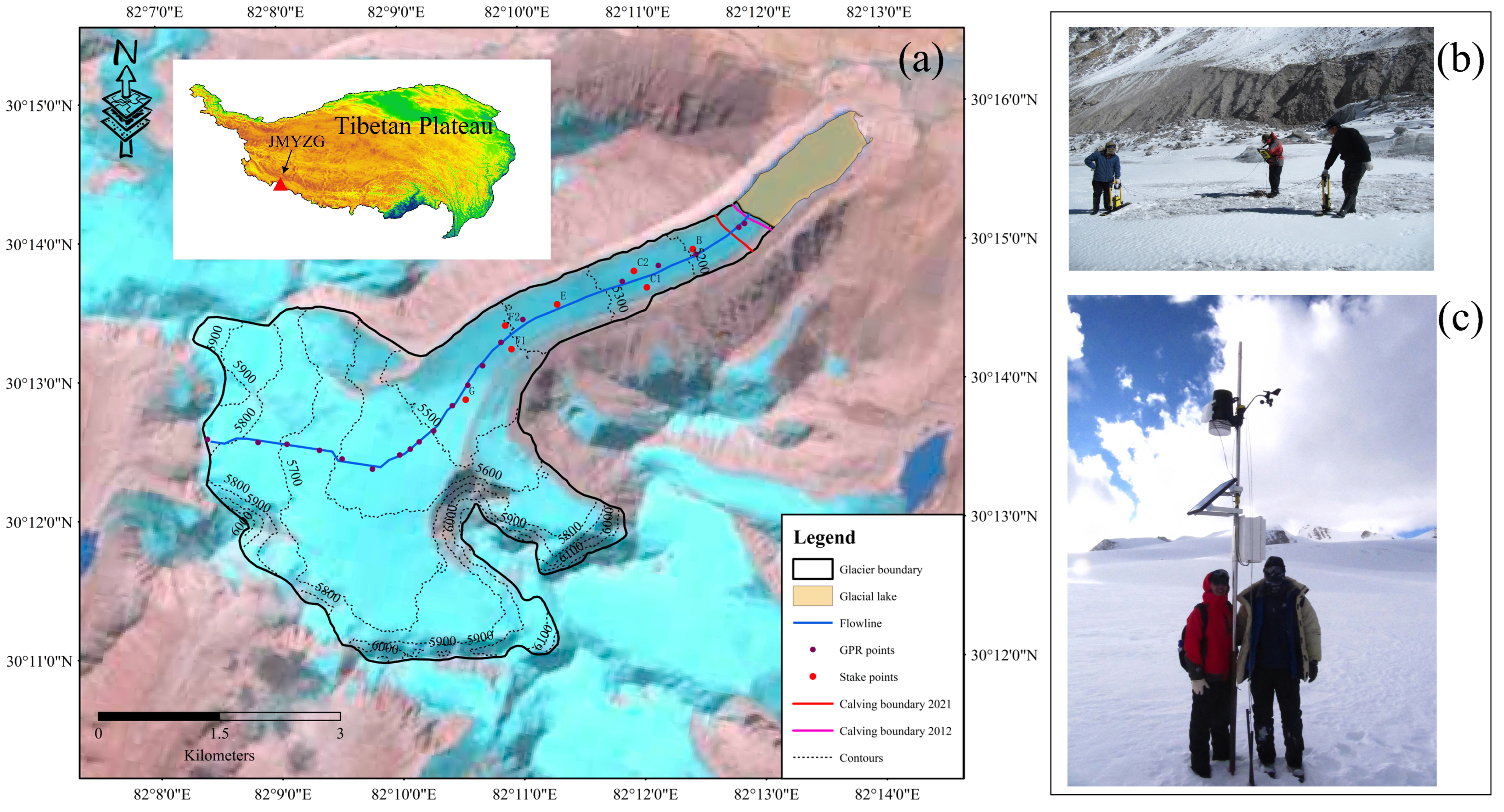
2. Study Area

JMYZG (Figure 1) is located in Zhongba County, Tibet, west of the Himalayas and southwest of the Tibetan Plateau (30°14′N, 82°12′E). It is the source of the Yarlung Zangbo River [26,29]. JMYZG has a total length of approximately 8 km, an area of approximately 20 km², and an altitude span of approximately 5100∼5900 m a.s.l. The glacier’s area decreased over the period from 1974 to 2010 with an increasing termini retreat rate [30]. Additionally, there still exists temperate ice in the upper area in JMYZG, although the glacier is at a high elevation [31].

3. Data and Methods

3.1. Data

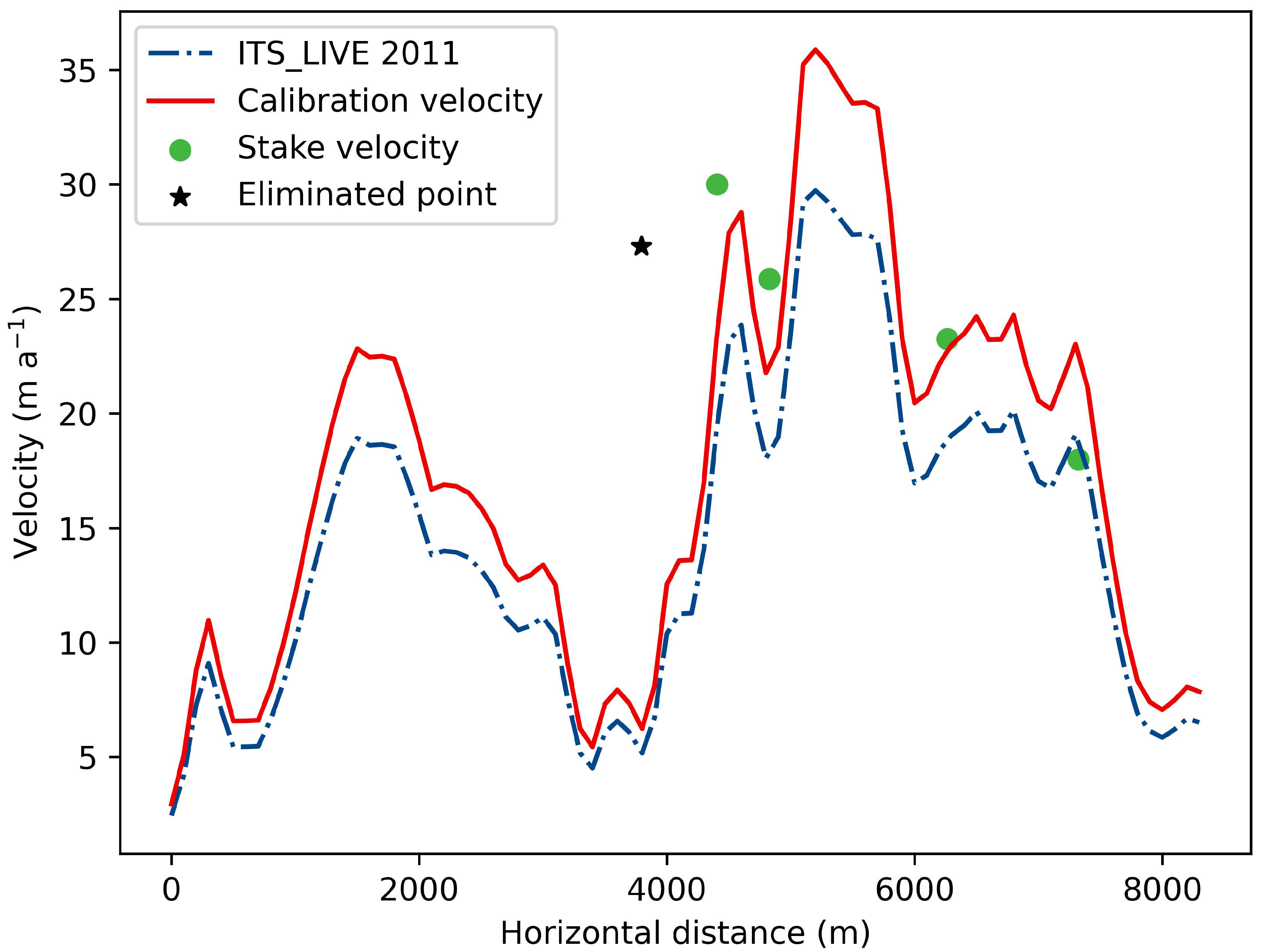
3.1.1. Surface Velocity

The surface velocity mainly includes in situ and publicly available glacier surface velocity datasets. The in situ data were acquired in the summer of 2011, and a total of 7 stakes were used for ice surface velocity observations (Figure 1). Due to the different acquisition times, measurement techniques, and so on, there exist certain errors between in situ and observational data. Furthermore, due to the small number of stakes, to achieve full coverage of the glacier surface, we additionally used them to calibrate the Inter-mission Time Series of Land Ice Velocity and Elevation (ITS_LIVE) data for JMYZG. ITS_LIVE is part of NASA’s Making Earth System Data Records for Use in Research Environments (MEaSUREs) 2017 project and includes yearly glacier surface velocity data from 1985 to 2018 with a spatial resolution of 240 m and a multi-year average resolution of 120 m [32]. Note that, since our in situ data were acquired during the field investigation in 2011, we also calibrated the ITS_LIVE data in 2011 to invert the basal friction coefficient [33]. Additionally, the surface elevation along the flowline was acquired by GPS.

The Robin inversion model needs to use the observational surface velocity as the boundary condition. Therefore, to invert the whole basal friction coefficient, we need the surface velocity covering the entire glacier. However, mountain glaciers are usually located in high-altitude areas, so it is difficult to obtain observational data due to the challenging logistics. During the field investigation in 2011, only a small amount of the surface observational velocity data were obtained by stakes in summer. Therefore, we calibrated the ITS_LIVE data by the stakes’ observational results. Similar to Zhang et al. [34], we multiplied the summer velocities by a correction factor of 0.75 to estimate the mean annual velocities. The detailed calibration method can be divided into the following three steps:

• Extracting the surface velocity of ITS_LIVE at the stakes;
• Calculating the ratio between the velocity at the stakes and the corresponding ITS_LIVE results in 2011. We used the Pauta criterion (3$\sigma$ principle, where $\sigma$ is the standard deviation) [35] to eliminate the stakes’ velocity containing large errors. Then, we took the mean of the remaining ratios as the correction factor;
• Finally, we applied the correction factor to ITS_LIVE to obtain the surface velocities covering the entire glacier.

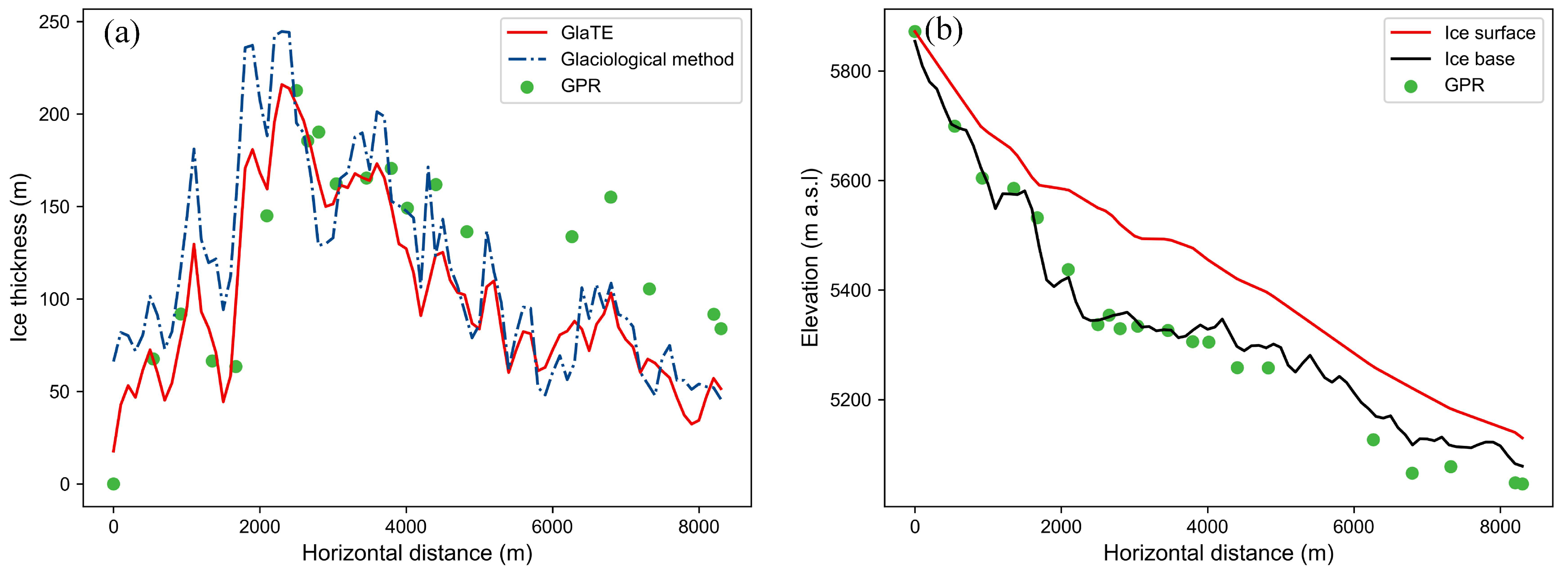
3.1.2. Ice Thickness

Similarly, the ice thickness data combine both the observation and model inversion data. The observational thickness data were obtained by a 5 M-frequency GPR during field investigations in 2011. However, the GPR points were only distributed along the flowline (Figure 1) and were relatively sparse. In addition, the temperate ice layer existing in mountain glaciers at high elevations [31,34,36] can also cause uncertainties in the GPR results. Therefore, we used the Glacier Thickness Estimation algorithm (GlaTE) inversion model [37] to acquire a more spatially continuous glacier geometry, and the in situ measured GPR data are an important constraint for the GlaTE.

Additionally, this model combines observational data (e.g., GPR measurements) with other glaciological ice thickness model constraints (e.g., Clarke et al., 2013 [38]). All constraints were formulated so that they can be integrated into a single system of equations, which can be solved with an appropriate solver; more details about the GlaTE are in Langhammer et al. [37].

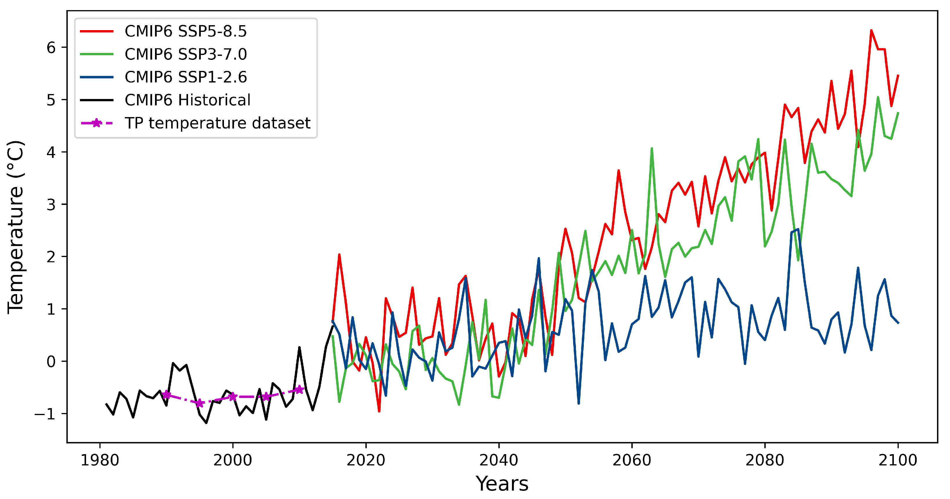
3.1.3. Surface Air Temperature

To approximate the future evolution of JMYZG under different climate scenarios, we used the surface temperature output from the Coupled Model Intercomparison Project Phase 6 (CMIP6) [39] in three different shared socioeconomic pathway (SSP) scenarios [40]. To have a more complete investigation of how JMYZG will respond to future climate changes, we chose two extreme climate scenarios (SSP1-2.6 and SSP5-8.5) as the upper and lower bound and a medium climate scenario (SSP3-7.0) to parameterize the surface mass balance (SMB) of JMYZG. Then, we used the SMB to drive our ice flow model to investigate its climate sensitivity. To make the CMIP6 air temperature more in line with the observed air temperature in the study area, we used the mean Tibetan Plateau surface air temperature dataset [41] for JMYZG to calibrate the CMIP6 air temperature outputs. This dataset records the spatial distribution of changes in the annual mean temperature in the Tibetan Plateau every five years from 1990 to 2015, with a spatial resolution of 1 km. Additionally, the global climate model (GCM) used in this study is GFDL-ESM4 [42], and we used a bilinear interpolation method to resample the CMIP6 temperature data in JMYZG.

Considering that JMYZG has no observational SMB data, we used the SMB gradient [43,44,45] to parameterize the SMB. This parameterization scheme requires less data and can obtain the SMB of the entire glacier using only air temperature as an input. This method is widely used in the study of glacier evolution in the HMAs [46,47,48]. Similar to Zhao et al. [46], we used a relatively simple parameterization scheme for the SMB as

$$SMB={\beta }_1(h_s-h_{ELA}),$$

(1)

where ${\beta }_1$ (m a${}^{-1}$ m${}^{-1}$) is the SMB gradient, which is a time-independent constant. The SMB gradient was set as a constant 0.0038 from Naimona’nyi Glacier (30°27′N, 81°20′E) near JMYZG [46,47]. The distance between Naimona’nyi Glacier and JMYZG is approximately 83 km, and both glaciers are located on the northern slope of the Himalayas and have similar climatic conditions. Moreover, $h_s$ is the surface elevation, and $h_{ELA}$ is the equilibrium-line altitude (ELA). In addition, the variation of the ELA with the change in air temperature can be expressed as [49]

$$\Delta h_{ELA}=\frac{\Delta T_S}{{\gamma }_T}.$$

(2)

where ${\gamma }_T$ represents the temperature lapse rate, which is set to a constant of −0.0072 °C m${}^{-1}$ [50], $\Delta T_S$ is the change of surface air temperature relative to the initial time (2011) in JMYZG, and $\Delta h_{ELA}$ represents the change in ELA.

The surface temperature of JMYZG and the change relative to the initial time can be obtained by interpolating the output of the CMIP6 temperature. By specifying the initial ELA, the parameterization of the SMB can be achieved. In addition, the initial ELA was obtained by Landsat-5 TM images at the end of the ablation season in 2011 and the Shuttle Radar Topography Mission (SRTM) digital elevation model (DEM) in 1 arc (approximately 30 m), which was approximately 5465 m. Due to the uncertainty of the CMIP6 air temperature output, we used the surface air temperature data obtained from the Tibetan Plateau air temperature dataset [41] from 1990 to 2010 to calibrate the historical temperature of CMIP6 and applied the calibration to the future results of CMIP6. Additionally, there is a pro-glacial lake connecting to the terminus of JMYZG; we then estimated the calving rate through the retreat distance (Figure 1) and parameterized it as part of the SMB to better simulate the retreat of the terminus.

3.2. Methods

3.2.1. Ice Flow Model

We used a 2D Blatter–Pattyn model of glacier flow along the flowline named the Polythermal Land Ice Model (PoLIM) [28]. This model assumes hydrostatic approximation for vertical normal stress and neglects the terms including the horizontal derivatives of vertical velocity in the viscous rheology of ice and the momentum equation [51,52]. We took x as the along-flowline horizontal coordinate, y as the transverse coordinate, and z as the vertical coordinate. The momentum balance equation is described by [53]

$$\frac{\partial }{\partial x}\left(2{\tau }_{xx}+{\tau }_{yy}\right)+\frac{\partial {\tau }_{xy}}{\partial y}+\frac{\partial {\tau }_{xz}}{\partial z}={\rho }_{i}g\frac{\partial s}{\partial x},$$

(3)

where ${\tau }_{ij}(i,j=x,y,z)$ represents the deviatoric stress tensor component, ${\rho }_i$ is the ice density, s is the ice surface, and g is the gravitational acceleration. The ice rheology can be described by the constitutive equation [54]

$${\tau }_{ij}=2\eta {\dot{ϵ}}_{ij},$$

(4)

where ${\dot{ϵ}}_{ij}$ is the strain rate tensor and ${\dot{ϵ}}_{ij}=\partial u_i/\partial x_j$. $\eta$ is the viscosity of ice and can be calculated as [54]

$$\eta =\frac{1}{2}{A}^{-1/n}{\dot{ϵ}}_e^{(1-n)/n},$$

(5)

where n is the creep exponent, A is the flow rate factor, and ${\dot{ϵ}}_e$ is the effective strain rate. Ground penetrating radar measurements suggested that most of the JMYZG ice is temperate [31]. We therefore assumed the entire glacier as an isothermal body in this simulation, and we set $A={10}^{-16}$ Pa${}^{-3}$ a${}^{-1}$, which corresponds roughly to the value at −2 °C.

The lateral drag and the lateral velocity gradient are parameterized by the half-width W following [55]

$${\tau }_{xy}=-\frac{\eta u}{W},\frac{\partial v}{\partial y}=\frac{u}{W}\frac{\partial W}{\partial x},$$

(6)

where u and v represent the horizontal velocities. The glacier width along the flowline is calculated by intersecting the normals at each node with the glacier outline. The along-flowline momentum equation can be reformulated in terms of horizontal velocity u as

$$\begin{array}{c}\frac{u}{W}\left\{2\frac{\partial \eta }{\partial x}\frac{\partial W}{\partial x}+2\eta \left[\frac{{\partial }^{2}W}{\partial x^2}-\frac{1}{W}{\left(\frac{\partial W}{\partial x}\right)}^2\right]-\frac{\eta }{W}\right\}+\frac{\partial u}{\partial x}\left(4\frac{\partial \eta }{\partial x}+\frac{2\eta }{W}\frac{\partial W}{\partial x}\right)+\\ \frac{\partial \eta }{\partial z}\frac{\partial u}{\partial z}+4\eta \frac{{\partial }^{2}u}{\partial x^2}+\eta \frac{{\partial }^{2}u}{\partial z^2}={\rho }_{i}g\frac{\partial s}{\partial x}.\end{array}$$

(7)

To make the partial differential Equation (7) a solvable problem, surface and basal boundary conditions should be set [52]. The ice surface was assumed to be stress-free:

$$\left(4\frac{\partial u}{\partial x}+\frac{2u}{W}\frac{\partial W}{\partial x}\right)\frac{\partial s}{\partial x}-\frac{\partial u}{\partial z}=0.$$

(8)

In addition, for the basal boundary condition, we used a linear friction law:

$${\tau }_b={\beta }^2{u}_b,$$

(9)

where ${\tau }_b$ is the basal drag, ${\beta }^2$ is the basal friction coefficient, and $u_b$ is the basal sliding velocity. To perform prognostic simulations under different climate scenarios, the thickness evolution of the glacier is governed by [28]:

$$\frac{\partial H}{\partial t}=-\frac{1}{W}\frac{\partial \left(\overline{u}HW\right)}{\partial x}+m_s,$$

(10)

where H is the ice thickness and t is the time step of the ice flow model, which was set to 1 year. Note that $m_s$ is the surface mass balance (SMB). Here, we used parameterized SMB results under different climate scenarios of CMIP6 to force the ice flow model for climate sensitivity experiments.

3.2.2. Robin Inversion

The basal sliding parameter ${\beta }^2$ in Equation (9) cannot be observed directly. Therefore, we obtained ${\beta }^2$ by the Robin inversion model [33]. As mentioned in Section 3.2.1, the surface boundary condition is generally set to stress-free boundary conditions. Furthermore, the surface velocity observed by satellites can be used as the Dirichlet boundary condition. Then, different velocities can be obtained by applying different surface boundary conditions in the ice flow model, i.e., $v^N$ and $v^D$. Therefore, a cost function $J\left(\beta \right)$ can then be constructed as [33]

$$J\left(\beta \right)={\int }_{{\Gamma }_b}2\beta {\left|{\mathbf{v}}^N-{\mathbf{v}}^D\right|}_F^2,$$

(11)

where ${\Gamma }_b$ represents the ice base and F represents the F-norm. We used an iterative method to obtain the minimum of J, and the convergence condition can be simply expressed as

$$\left|J^{n+1}-J^n\right|\le \epsilon ,$$

(12)

where $J^n$ represents the value of the cost function in the nth iteration and $\epsilon$ is the termination criterion, which was set to ${10}^{-2}$ in this experiment. When this criterion is satisfied, we consider the function $J\left(\beta \right)$ to have converged. Finally, we can obtain the inversion results of the basal friction coefficient ${\beta }^2$. More details are discussed in Arthern et al. [33].

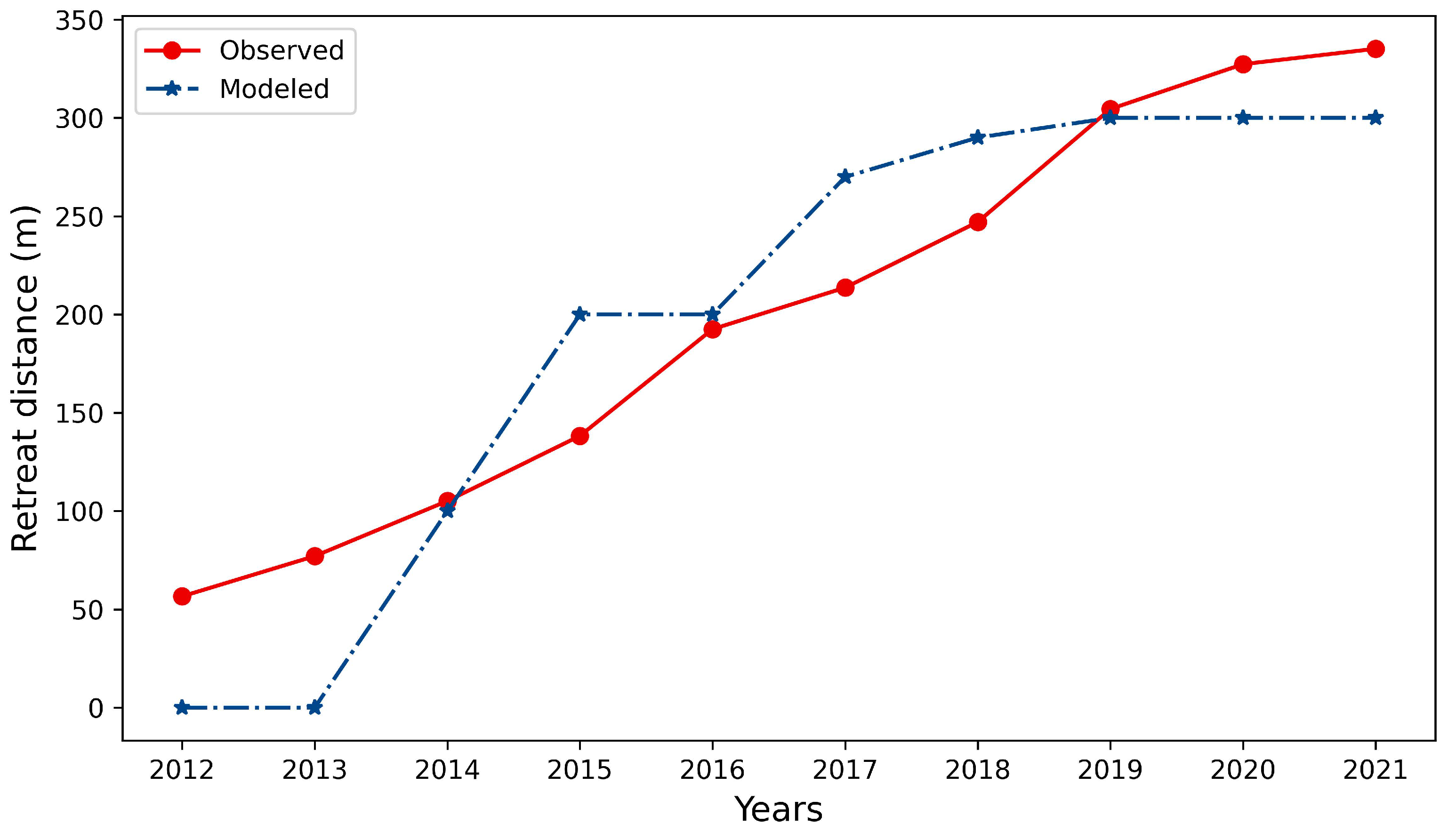
3.3. Validation of the Retreat of Glacier Termini

To accurately simulate the future evolution of JMYZG, it is necessary to use the ice flow model to reconstruct the historical evolution state of the glacier. Considering that there is a glacial lake at the termini of JMYZG causing continuous mass loss, we used Landsat satellite images to estimate the mean annual calving rate from 2011 to 2021 and took it as a part of the ablation at the termini of the glacier. Similar to Skvarca et al. [56], we parameterized the SMB using the water depth of the glacial lake, and the calving rate was calculated as

$$u_c=u_t+\frac{\Delta L}{\Delta t},$$

(13)

where $u_c$ is the calving rate and $u_t$ is the surface velocity at the termini, which is approximately 5 m a${}^{-1}$. $\Delta$L is the retreat distance, and $\Delta t$ is the observation time. Additionally, $\Delta L$/$\Delta t$ represents the mean annual retreat rate over the 10-year period (2011–2021), which is approximately 33 m a${}^{-1}$. Therefore, $u_c$≈ 38 m a${}^{-1}$. We assumed that the calving rate is proportional to the depth of the ice lake [56] as

$$u_c=c\times H_W,$$

(14)

where $H_W$ represents the lake depth at the terminus of the glacier, which is approximately 49 m, and we can calculate the c proportionality coefficient, which is approximately 0.77 m a${}^{-1}$ m${}^{-1}$ in this study. The depth of the terminal glacial lake was obtained from the lake height, which was approximately obtained from the 30 m SRTM DEM and the bedrock elevation of the termini obtained from the GPR data. Next, we can convert the calving rate to the equivalent termini’s surface mass balance $SM{B}_c$. It can be calculated as

$$u_c\times {\overline{H}}_t=\Delta L_1\times SM{B}_c,$$

(15)

which can be written as

$$SM{B}_c=u_c\frac{{\overline{H}}_t}{\Delta L_1},$$

(16)

where ${\overline{H}}_t$ represents the mean ice thickness at the termini and $\Delta L_1$ is the retreat distance from 2011 to 2012, which are approximately 40 and 56 m, respectively. Then, according to Equations (14) and (16), the parameterization of the SMB at the termini can be conducted through different depths of the glacial lake. Note that, in future simulations, once the elevation of ice base is higher than the lake surface, the termini’s calving will not be considered.

4. Results

4.1. Glacier Geometry

The inversion result of the thickness of JMYZG is shown in Figure 2. It can be seen that the difference of the ice thickness among the GPR data, the glaciological method that calculates the ice thickness by basal shear stress, as well as the surface slope acquired from DEM [38] and the GlaTE [37] result in the middle and upstream being in good agreement, while the downstream is a little different. This is because there were more GPR points in the upstream region, but sparse in the downstream region, resulting in fewer points constrained by the GlaTE. In addition, it could be an error caused by temperate ice. Overall, the three methods showed a similar spatial variation trend (Figure 2a). In addition, the surface elevation of JMYZG was obtained by the interpolation of the GPR points. Through the surface elevation and glacier thickness, we can obtain a relatively continuous spacial geometry of JMYZG. We found that JMYZG showed a trend of being thinner at the ends and thicker in the middle. The maximum ice thickness was found at a horizontal distance of approximately 2.3 km from the glacier head, which is approximately 215 m (Figure 2b).

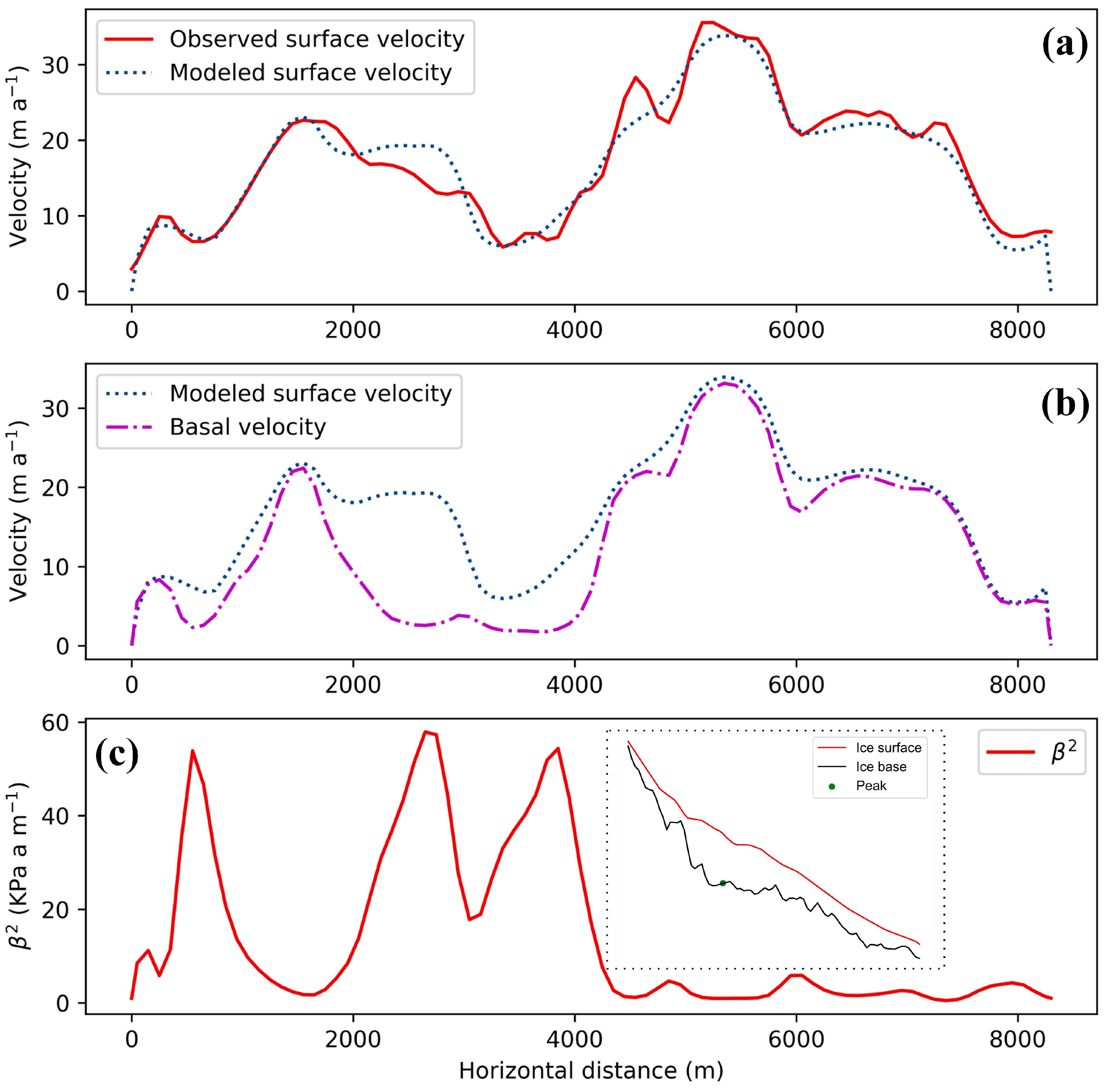
4.2. Basal Friction Coefficient

Once we obtain the glacier geometry, the basal friction coefficient can then be inverted by the ice flow model. As shown in Figure 3, in general, the measured velocities by the stakes were slightly larger than ITS_LIVE in 2011 (initial state in ice flow model). We used four stakes (the green solid points in Figure 3) to calibrate the ITS_LIVE data (the blue dash-dotted line in Figure 3). One of the stakes had a large gap with the ITS_LIVE data, and it was eliminated in our calibration procedure (the black star point in Figure 3). Then, we obtained the initial surface velocities in our simulation (the red solid line in Figure 3), which was applied in the Robin inversion. The maximum velocity was approximately 35 m a${}^{-1}$, and it showed a trend of being large in the middle and small at the terminals, which is similar to the distribution of the ice thickness (Figure 2).

The friction coefficient obtained by the Robin inversion is shown in Figure 4. We can see that the modeled surface velocities are in good agreement with the observed velocity (ITS_LIVE data after calibration; Figure 4a). In addition, the sliding velocities show a similar trend with the surface velocities; that is, the velocities are larger in the middle and relatively smaller at the terminus. The maximum sliding velocity was approximately 33 m a${}^{-1}$, where the horizontal distance was approximately 5.4 km (Figure 4b). Moreover, the basal friction coefficients are inversely proportional to the sliding velocities. The larger the friction coefficient is, the greater the resistance that will be produced, causing smaller sliding velocities (Figure 4c). The maximum of ${\beta }^2$ is approximately 57.9 KPa a m${}^{-1}$, located at the horizontal distance of approximately 2.7 km, where the corresponding sliding velocity is only 2.5 m a${}^{-1}$.

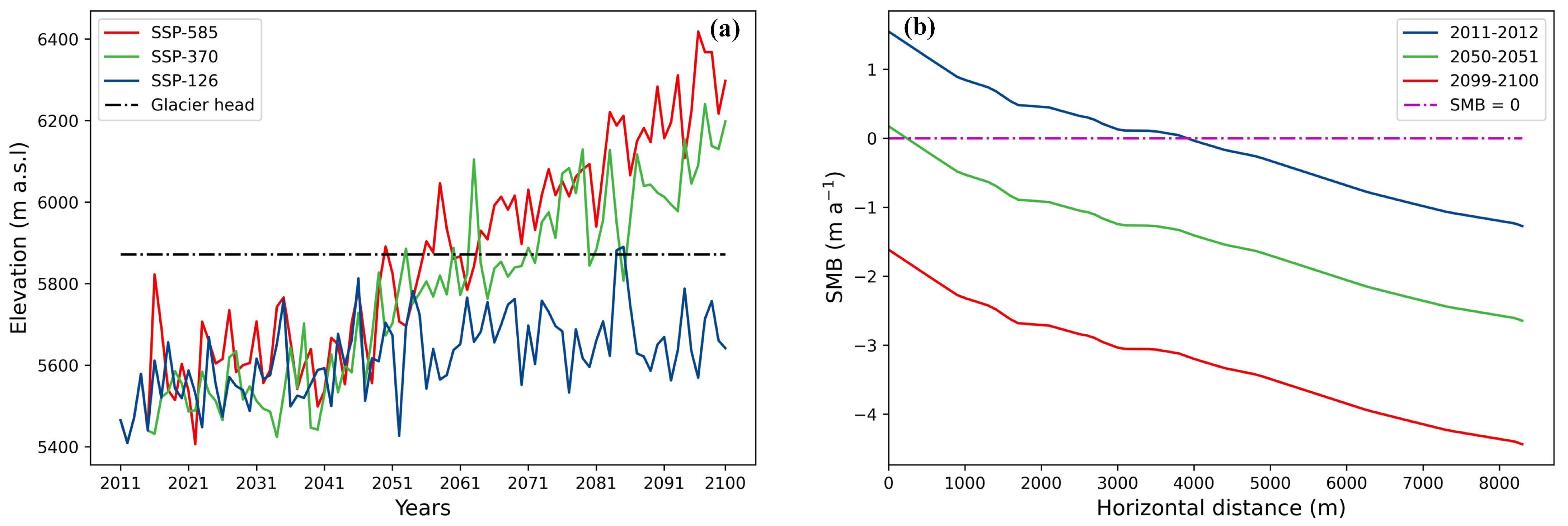
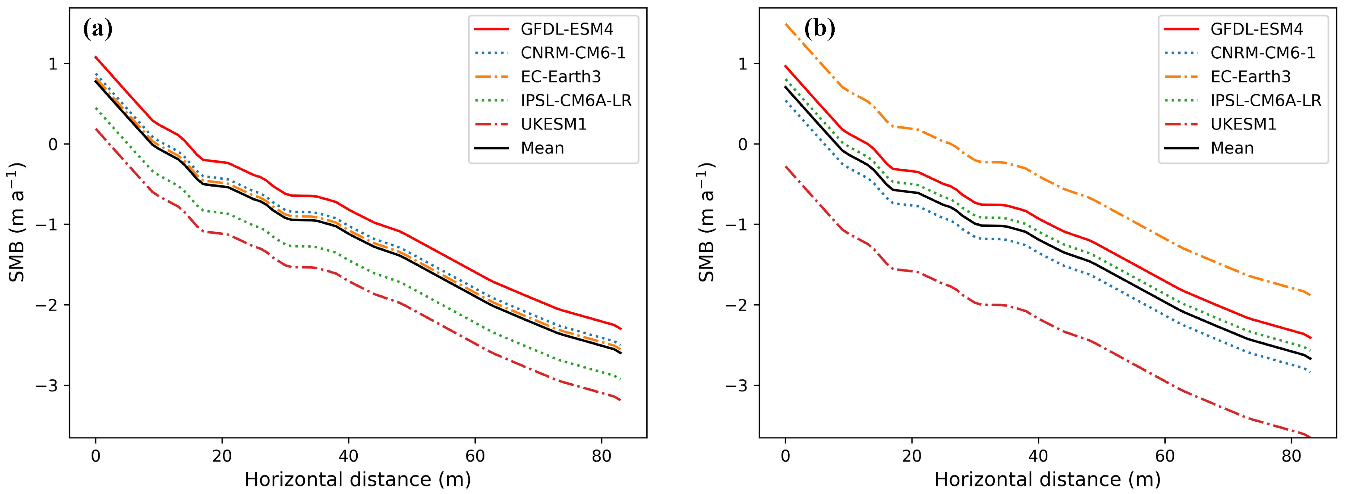
4.3. Surface Mass Balance

We used the surface air temperature and the change in the ELA to parameterize the SMB for JMYZG. As mentioned in Section 3.1.3, the surface air temperature after calibration is shown in Figure 5. We can see that after calibration, the CMIP6 temperature outputs are in good agreement with the temperature obtained by the interpolation of the Tibetan Plateau dataset [41]. Under the SSP1-2.6 scenario, the change of surface temperature in JMYZG is relatively stable, with an annual mean temperature of approximately 0.7 °C in 2100. However, under the scenario of SSP5-8.5, the mean annual temperature increases rapidly, rising to approximately 5.4 °C in 2100. Therefore, in SSP5-8.5, JMYZG is expected to retreat and lose mass quickly. Additionally, before 2050, the temporal sensitivity of temperature changes is relatively lower; there is not much difference in the temperature output under the different CMIP6 climate scenarios; however, the difference gradually increases after approximately 2050.

Figure 6 shows the time series change in the ELA under different climate scenarios, as well as the parameterization results of the SMB under SSP5-8.5. We can see that, under the high emission scenario (SSP5-8.5), the ELA increases rapidly; by approximately 2050, the ELA is higher than the glacier head, indicating that the entire glacier is completely in the ablation area along the flowline used in the ice flow model. Note that the SMB shown in Figure 6 does not take the termini’s calving by the glacial lake into account. When there is a terminal glacial lake, the SMB equivalent to calving needs to be added to the terminal surface mass balance. More details are described in Section 3.3.

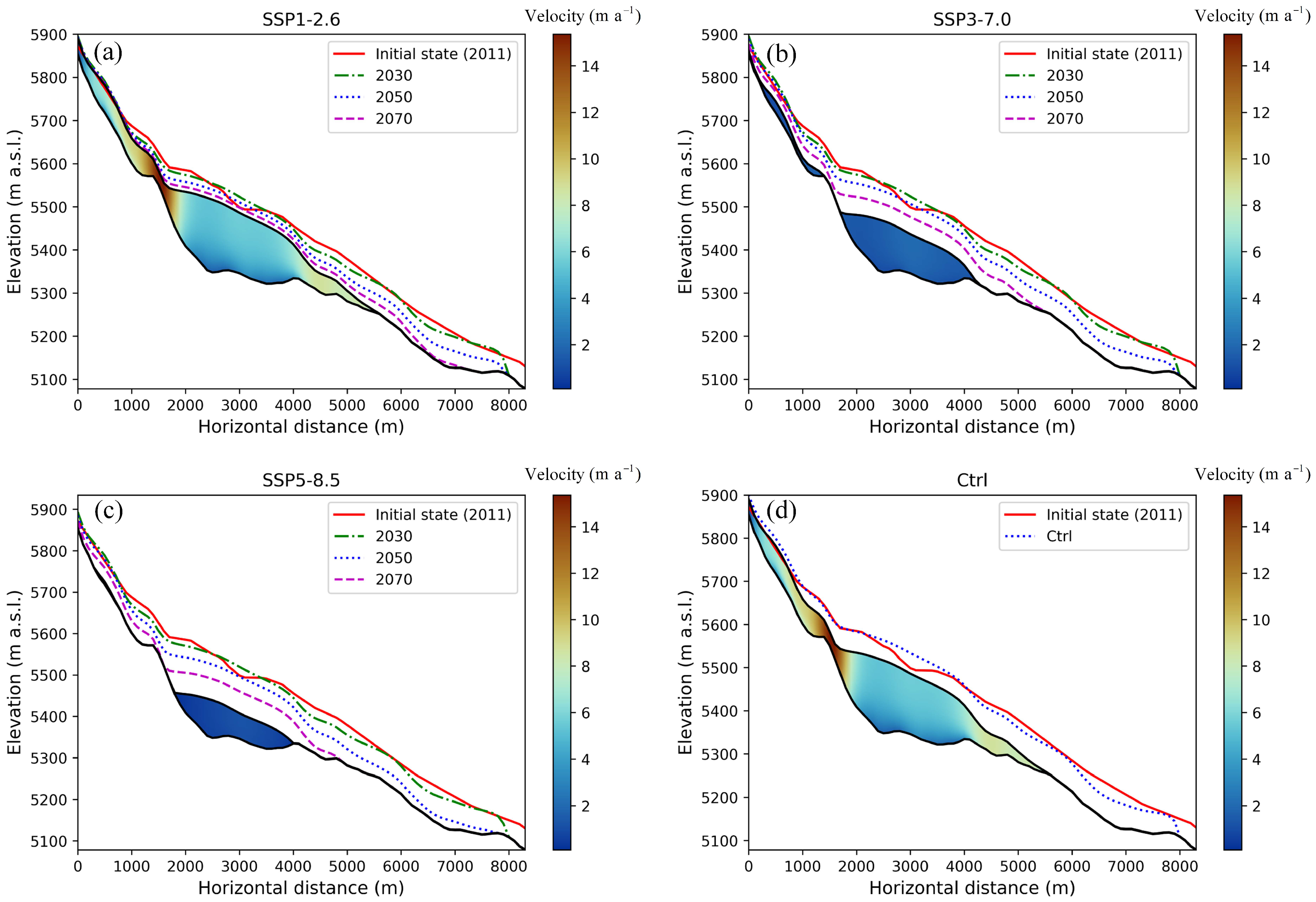
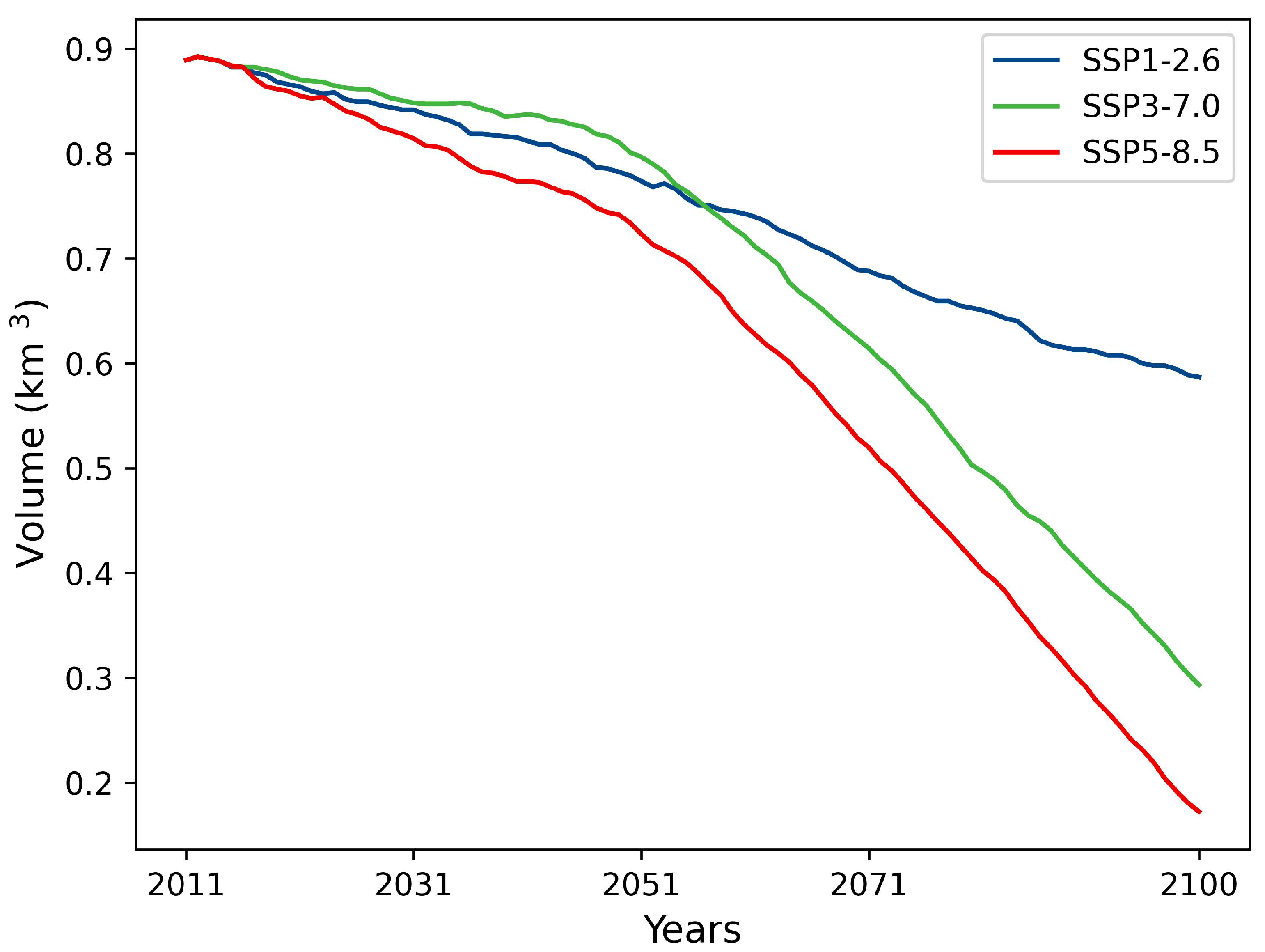
4.4. Future Evolution

To predict the future evolution, it is necessary to use the ice flow model to reconstruct the historical evolution state of the glacier. As mentioned in Section 4.3, due to the low time sensitivity of the CMIP6 air temperature output before 2050, there are smaller differences in the changes of the ELA under different climate scenarios. Therefore, we used the SMB under SSP1-2.6 to verify the simulation result in JMYZG by comparing the model outputs with the retreat distance observed from satellite images. Such a validation method has also been successfully applied to the simulation of outlet glaciers (e.g., Lea et al., 2014; Guo et al., 2019; Barnett et al., 2022 [57,58,59]), which gives us more confidence in projecting the future evolution of this glacier. From Figure 7, we can see that the modeled retreat distance is in good agreement with the observed distance. The glacier termini gradually retreated by approximately 300 m from 2011 to 2021. This proved the reliability of our simulation results by PoLIM, and the future dynamic simulation of JMYZG can continue to be carried out in this state.

In the future evolution simulations, we used the SMB under different CMIP6 climate scenarios to drive the ice flow model to investigate the climate sensitivity for JMYZG. The simulation results are shown in Figure 8. It can be seen that the glacier surface elevations under different scenarios from 2030 to 2050 are basically the same (the green dash-dotted line and blue dotted lines in Figure 8a–c, respectively). However, the difference in the surface elevation of JMYZG increases in different scenarios over time, i.e., from 2050 to 2070 (blue dotted and magenta dashed lines in Figure 8a–c, respectively), there is a more significant difference in the simulations under different climate scenarios. Finally, the difference reaches a maximum in 2100. Furthermore, we conducted a “control” experiment to keep the SMB fixed. It can be seen that, in the control experiment, compared with the initial state, the glacier thickness will increase in the midstream and decrease in the termini in 2100, and the ice thickness of the control experiment is larger than that of SSP1-2.6 in 2100 (Figure 8d). In addition, we assumed the glacier as a U-shaped valley to estimate its time series of volume under different climate scenarios (Figure 9). In our simulations, the glacier volume first increased slightly and then decreased, and the mass loss will intensify after approximately 2050. From Figure 6 the ELA gradually increases over time, and the extent of the ablation area increases. Therefore, the change of glacier volume is in good agreement with the changes in the ELA. Additionally, under SSP5-8.5, the entire JMYZG will lose as much as approximately 81% mass by 2100, while under SSP1-2.6, the mass loss speed is relatively small, i.e., approximately 34%.

5. Discussion

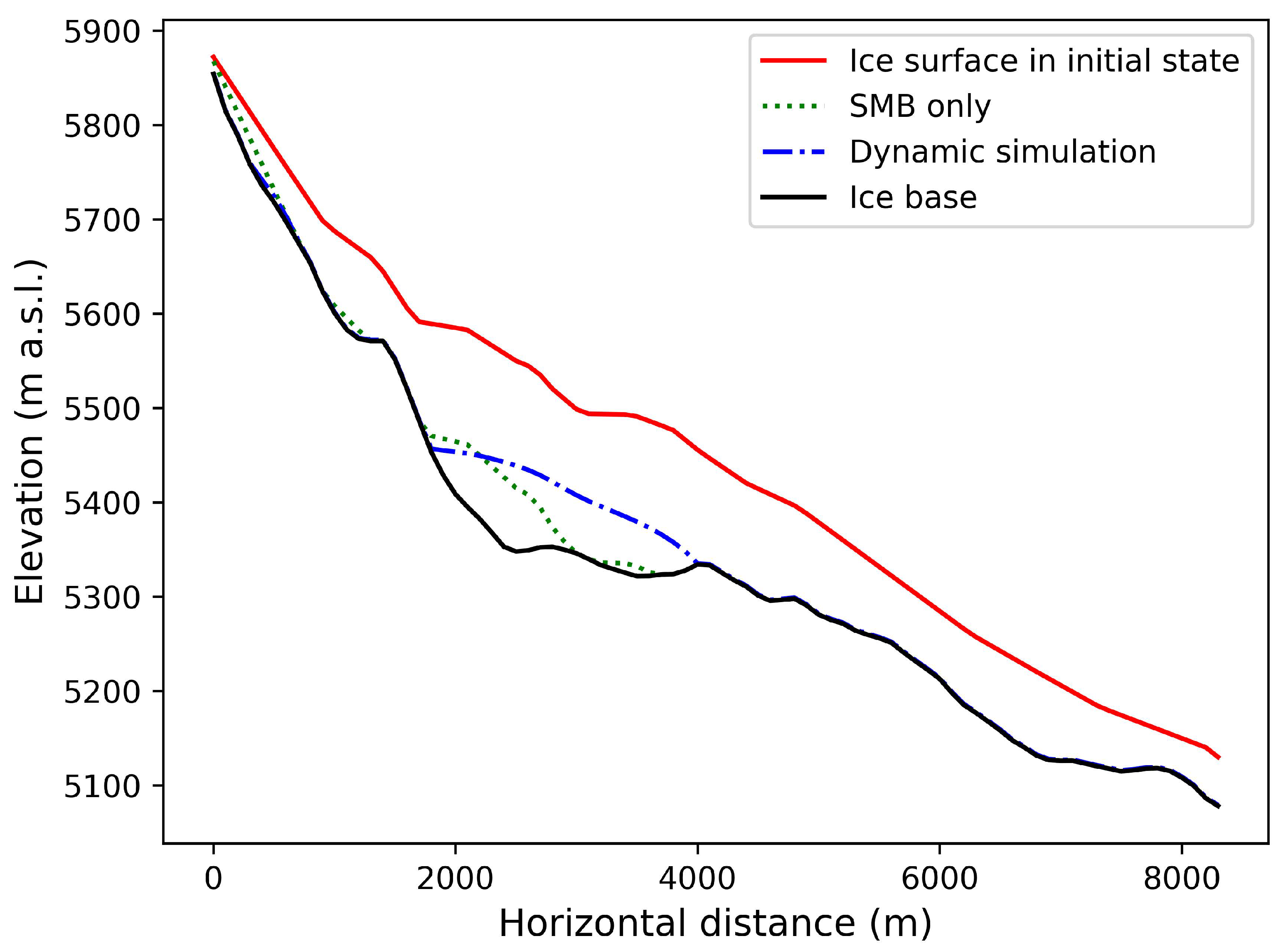
5.1. Dynamic Feature

In order to estimate the influence of the “ice dynamics”, we compared the simulation results with (simulated by the numerical ice flow model PoLIM) and without dynamic features (simulated just by the SMB). We further investigated the evolution of the glacier surface under the above two conditions under SSP5-8.5 as Figure 10. We can see that the dynamic features have an obvious influence on the evolution of the glacier, that is, when the glacier flow is taken into account, ice from the upper reaches of the glacier flows downwards under the force of gravity and acts as a supply for the lower reaches, so the elevation of the ice surface is higher than it would be if only the SMB is taken into account. This suggests that using only the SMB to investigate the evolution of glaciers may overestimate the mass loss of glaciers. Of course, this “overestimation” may not be universal and is only a special case of the current simulation of JMYZG. Nevertheless, this is enough to show that it is valuable to consider the dynamic features of glaciers in simulations.

5.2. Model Uncertainty

Finally, in this study, due to the sparsity of observational data, we used the relatively simple SMB gradient method to parameterize the SMB, which requires the temperature output of the CMIP6 model as the input. The global climate model used in this study is GFDL-ESM4. It is a coupled chemistry–carbon–climate Earth system model developed by the physical Fluid Dynamics Laboratory and provides model outputs to the sixth phase of the Coupled Model Intercomparison Project (CMIP6) [42]. To estimate the model uncertainties raised by climate forcings, we compared the parameterized SMB results in 2060 and 2100 for GFDL-ESM4, CNRM-CM6-1 [60], EC-Earth3 [61], IPSL-CM6A-LR [62], and UKESM1 [63], under the SSP1-2.6 scenario, as in Figure 11. It can be seen that there are still great uncertainties in the simulation results among different models. For example, in 2060, we see the largest SMB difference (0.9 m a${}^{-1}$) between GFDL-ESM4 and UKESM1 (Figure 11a). However, in 2100, the largest SMB difference (1.3 m a${}^{-1}$) can be found between EC-Earth3 and UKESM1 (Figure 11b). Therefore, the uncertainties of the SMB is one of the uncertainty sources in our model results. In addition, the 2D models have inherent errors, which cannot reflect the realistic evolution of glacier like the three-dimensional (3D) ice flow models. Note that the flowline in this study is not the main flowline from the perspective of glaciology; it is just the flowline used in our modeling. Thus, the modeled volume change may mismatch with the realistic evolution of the glacier.

6. Conclusions

Mountain glaciers are usually located in high altitude where there are sparse observational data. In this study, we used a higher-order ice flow model to simulate the evolution of Jiemayangzong Glacier (JMYZG), the headstream of the Yarlung Zangbo River, which is an important water source in many domestic and agricultural practices [64,65]. We took the inversion of the ice thickness and friction coefficient as the initial parameters and used the latest CMIP6 air temperature outputs to parameterize the glacier surface mass balance as the climate forcing to investigate the response of JMYZG to the future climate changes. The reliability of the simulation was validated by comparing the retreat distance of the termini in the historical period with satellite observations. We found that, under the SSP5-8.5 climate scenario and with a drastic ablation rate, JMYZG experienced a volume loss of approximately 81% from 2011∼2100, while the volume loss was relatively slower under SSP1-2.6, i.e., approximately 34% by 2100. In addition, through our numerical simulation results, we found that, regardless of the climate scenario, JMYZG will retreat consistently, and the retreat rate will increase after approximately 2050. This study is beneficial for furthering the understanding of the physical processes of mountain glaciers in the Himalayas and can also provide a theoretical basis for local disaster prevention and water resource management. Note that, due to the sparse in situ observational data, we used a relatively simple parameterization method of the SMB, and a limited number of stakes were used to calibrate the surface velocity of the entire glacier. All these factors led to an increase in model uncertainty. How to overcome the influence of these uncertainties and improve the accuracy of numerical models of mountain glaciers still need further efforts.

References

- Oerlemans, J.; Anderson, B.; Hubbard, A.; Huybrechts, P.; Johannesson, T.; Knap, W.; Schmeits, M.; Stroeven, A.; Van de Wal, R.; Wallinga, J.; et al. Modelling the response of glaciers to climate warming. Clim. Dyn. 1998, 14, 267–274. [Google Scholar] [CrossRef]
- Haeberli, W.; Hoelzle, M.; Paul, F.; Zemp, M. Integrated monitoring of mountain glaciers as key indicators of global climate change: The European Alps. Ann. Glaciol. 2007, 46, 150–160. [Google Scholar] [CrossRef]
- Post, A.; O’Neel, S.; Motyka, R.J.; Streveler, G. A complex relationship between calving glaciers and climate. Eos Trans. Am. Geophys. Union 2011, 92, 305–306. [Google Scholar] [CrossRef]
- IPCC. IPCC Climate Change 2021: The Physical Science Basis; Masson-Delmotte, V., Zhai, P., Pirani, A., Connors, S.L., Péan, C., Berger, S., Gaud, N., Chen, Y., Goldfarb, L., Gomis, M.I., et al., Eds.; Cambridge University Press: Cambridge, UK, 2021; in press. [Google Scholar]
- Fox-Kemper, B.; Hewitt, H.; Xiao, C.; Aðalgeirsdóttir, G.; Drijfhout, S.; Edwards, T.; Golledge, N.; Hemer, M.; Kopp, R.; Krinner, G.; et al. Ocean, Cryosphere and Sea Level Change Supplementary Material. In Climate Change 2021: The Physical Science Basis; Contribution of Working Group I to the Sixth Assessment Report of the Intergovernmental Panel on Climate Change; Cambridge University Press: Cambridge, UK, 2021; in press. [Google Scholar]
- Milner, A.M.; Khamis, K.; Battin, T.J.; Brittain, J.E.; Barrand, N.E.; Füreder, L.; Cauvy-Fraunié, S.; Gíslason, G.M.; Jacobsen, D.; Hannah, D.M.; et al. Glacier shrinkage driving global changes in downstream systems. Proc. Natl. Acad. Sci. USA 2017, 114, 9770–9778. [Google Scholar] [CrossRef]
- Purdie, H. Glacier retreat and tourism: Insights from New Zealand. Mt. Res. Dev. 2013, 33, 463–472. [Google Scholar] [CrossRef]
- Stewart, E.J.; Wilson, J.; Espiner, S.; Purdie, H.; Lemieux, C.; Dawson, J. Implications of climate change for glacier tourism. Tour. Geogr. 2016, 18, 377–398. [Google Scholar] [CrossRef]
- Bhattacharya, A.; Bolch, T.; Mukherjee, K.; King, O.; Menounos, B.; Kapitsa, V.; Neckel, N.; Yang, W.; Yao, T. High Mountain Asian glacier response to climate revealed by multi-temporal satellite observations since the 1960s. Nat. Commun. 2021, 12, 4133. [Google Scholar] [CrossRef]
- Zhang, M.; Chen, F.; Zhao, H.; Wang, J.; Wang, N. Recent Changes of Glacial Lakes in the High Mountain Asia and Its Potential Controlling Factors Analysis. Remote Sens. 2021, 13, 3757. [Google Scholar] [CrossRef]
- Shugar, D.H.; Burr, A.; Haritashya, U.K.; Kargel, J.S.; Watson, C.S.; Kennedy, M.C.; Bevington, A.R.; Betts, R.A.; Harrison, S.; Strattman, K. Rapid worldwide growth of glacial lakes since 1990. Nat. Clim. Chang. 2020, 10, 939–945. [Google Scholar] [CrossRef]
- Zhang, G.; Yao, T.; Xie, H.; Wang, W.; Yang, W. An inventory of glacial lakes in the Third Pole region and their changes in response to global warming. Glob. Planet. Chang. 2015, 131, 148–157. [Google Scholar] [CrossRef]
- Nie, Y.; Sheng, Y.; Liu, Q.; Liu, L.; Liu, S.; Zhang, Y.; Song, C. A regional-scale assessment of Himalayan glacial lake changes using satellite observations from 1990 to 2015. Remote Sens. Environ. 2017, 189, 1–13. [Google Scholar] [CrossRef]
- King, O.; Bhattacharya, A.; Bhambri, R.; Bolch, T. Glacial lakes exacerbate Himalayan glacier mass loss. Sci. Rep. 2019, 9, 18145. [Google Scholar] [CrossRef] [PubMed]
- Brun, F.; Wagnon, P.; Berthier, E.; Jomelli, V.; Maharjan, S.B.; Shrestha, F.; Kraaijenbrink, P.D.A. Heterogeneous Influence of Glacier Morphology on the Mass Balance Variability in High Mountain Asia. J. Geophys. Res. Earth Surf. 2019, 124, 1331–1345. [Google Scholar] [CrossRef]
- Pronk, J.B.; Bolch, T.; King, O.; Wouters, B.; Benn, D.I. Contrasting surface velocities between lake- and land-terminating glaciers in the Himalayan region. Cryosphere 2021, 15, 5577–5599. [Google Scholar] [CrossRef]
- Wei, J.; Liu, S.; Wang, X.; Zhang, Y.; Jiang, Z.; Wu, K.; Zhang, Z.; Zhang, T. Longbasaba Glacier recession and contribution to its proglacial lake volume between 1988 and 2018. J. Glaciol. 2021, 67, 473–484. [Google Scholar] [CrossRef]
- Liu, Q.; Mayer, C.; Wang, X.; Nie, Y.; Wu, K.; Wei, J.; Liu, S. Interannual flow dynamics driven by frontal retreat of a lake-terminating glacier in the Chinese Central Himalaya. Earth Planet. Sci. Lett. 2020, 546, 116450. [Google Scholar] [CrossRef]
- Tsutaki, S.; Fujita, K.; Nuimura, T.; Sakai, A.; Sugiyama, S.; Komori, J.; Tshering, P. Contrasting thinning patterns between lake- and land-terminating glaciers in the Bhutanese Himalaya. Cryosphere 2019, 13, 2733–2750. [Google Scholar] [CrossRef]
- Sato, Y.; Fujita, K.; Inoue, H.; Sakai, A.; Karma. Land- to lake-terminating transition triggers dynamic thinning of a Bhutanese glacier. Cryosphere 2022, 16, 2643–2654. [Google Scholar] [CrossRef]
- Carrivick, J.L.; Tweed, F.; Sutherland, J.L.; Mallalieu, J. Toward Numerical Modeling of Interactions Between Ice-Marginal Proglacial Lakes and Glaciers. Front. Earth Sci. 2020, 8, 577068. [Google Scholar] [CrossRef]
- Rounce, D.R.; Hock, R.; Shean, D.E. Glacier Mass Change in High Mountain Asia Through 2100 Using the Open-Source Python Glacier Evolution Model (PyGEM). Front. Earth Sci. 2020, 7, 331. [Google Scholar] [CrossRef]
- Kraaijenbrink, P.D.A.; Bierkens, M.F.P.; Lutz, A.F.; Immerzeel, W.W. Impact of a global temperature rise of 1.5 degrees Celsius on Asia’s glaciers. Nature 2017, 549, 257–260. [Google Scholar] [CrossRef] [PubMed]
- Maussion, F.; Butenko, A.; Champollion, N.; Dusch, M.; Eis, J.; Fourteau, K.; Gregor, P.; Jarosch, A.H.; Landmann, J.; Oesterle, F.; et al. The open global glacier model (OGGM) v1.1. Geosci. Model Dev. 2019, 12, 909–931. [Google Scholar] [CrossRef]
- Chen, C.; Zhang, L.; Xiao, T.; He, J. Barrier lake bursting and flood routing in the Yarlung Tsangpo Grand Canyon in October 2018. J. Hydrol. 2020, 583, 124603. [Google Scholar] [CrossRef]
- Sun, W.; Wang, Y.; Fu, Y.H.; Xue, B.; Wang, G.; Yu, J.; Zuo, D.; Xu, Z. Spatial heterogeneity of changes in vegetation growth and their driving forces based on satellite observations of the Yarlung Zangbo River Basin in the Tibetan Plateau. J. Hydrol. 2019, 574, 324–332. [Google Scholar] [CrossRef]
- Liu, S.; Wang, P.; Wang, C.; Wang, X.; Chen, J. Anthropogenic disturbances on antibiotic resistome along the Yarlung Tsangpo River on the Tibetan Plateau: Ecological dissemination mechanisms of antibiotic resistance genes to bacterial pathogens. Water Res. 2021, 202, 117447. [Google Scholar] [CrossRef]
- Wang, Y.; Zhang, T.; Xiao, C.; Ren, J.; Wang, Y. A two-dimensional, higher-order, enthalpy-based thermomechanical ice flow model for mountain glaciers and its benchmark experiments. Comput. Geosci. 2020, 141, 104526. [Google Scholar] [CrossRef]
- Ren, W.; Yao, T.; Xie, S. Water stable isotopes in the Yarlungzangbo headwater region and its vicinity of the southwestern Tibetan Plateau. Tellus B Chem. Phys. Meteorol. 2016, 68, 30397. [Google Scholar] [CrossRef]
- Liu, X.C.; Xiao, C.D. Preliminary Study of the Jiemayangzong Glacier and Lake Variations in the Source Regions of the Yarlung Zangbo River in 1974–2010. J. Glaciol. Geocryol. 2011, 33, 488–496. (In Chinese) [Google Scholar]
- Zhang, T.; Ding, M.; Xiao, C.; Zhang, D.; Du, Z. Temperate ice layer found in the upper area of Jima Yangzong Glacier, the headstream of Yarlung Zangbo River. Sci. Bull. 2016, 61, 619–621. [Google Scholar] [CrossRef]
- Gardner, A.; Fahnestock, M.; Scambos, T. MEaSUREs ITS_LIVE Landsat Image-Pair Glacier and Ice Sheet Surface Velocities: Version 1; NASA National Snow and Ice Data Center Distributed Active Archive Center: Boulder, CO, USA, 2021. [CrossRef]
- Arthern, R.J.; Gudmundsson, G.H. Initialization of ice-sheet forecasts viewed as an inverse Robin problem. J. Glaciol. 2010, 56, 527–533. [Google Scholar] [CrossRef]
- Zhang, T.; Xiao, C.; Colgan, W.; Qin, X.; Du, W.; Sun, W.; Liu, Y.; Ding, M. Observed and modelled ice temperature and velocity along the main flowline of East Rongbuk Glacier, Qomolangma (Mount Everest), Himalaya. J. Glaciol. 2013, 59, 438–448. [Google Scholar] [CrossRef]
- Zhao, X.; Jiang, N.; Liu, J.; Yu, D.; Chang, J. Short-term average wind speed and turbulent standard deviation forecasts based on one-dimensional convolutional neural network and the integrate method for probabilistic framework. Energy Convers. Manag. 2020, 203, 112239. [Google Scholar] [CrossRef]
- Wang, Y.; Zhang, T.; Ren, J.; Qin, X.; Liu, Y.; Sun, W.; Chen, J.; Ding, M.; Du, W.; Qin, D. An investigation of the thermomechanical features of Laohugou Glacier No. 12 on Qilian Shan, western China, using a two-dimensional first-order flow-band ice flow model. Cryosphere 2018, 12, 851–866. [Google Scholar] [CrossRef]
- Langhammer, L.; Grab, M.; Bauder, A.; Maurer, H. Glacier thickness estimations of alpine glaciers using data and modeling constraints. Cryosphere 2019, 13, 2189–2202. [Google Scholar] [CrossRef]
- Clarke, G.K.; Anslow, F.S.; Jarosch, A.H.; Radić, V.; Menounos, B.; Bolch, T.; Berthier, E. Ice volume and subglacial topography for western Canadian glaciers from mass balance fields, thinning rates, and a bed stress model. J. Clim. 2013, 26, 4282–4303. [Google Scholar] [CrossRef]
- Meehl, G.A.; Senior, C.A.; Eyring, V.; Flato, G.; Lamarque, J.F.; Stouffer, R.J.; Taylor, K.E.; Schlund, M. Context for interpreting equilibrium climate sensitivity and transient climate response from the CMIP6 Earth system models. Sci. Adv. 2020, 6, eaba1981. [Google Scholar] [CrossRef] [PubMed]
- IPCC. 2021: Summary for Policymakers. In Climate Change 2021: The Physical Science Basis; Masson-Delmotte, V., Zhai, P., Pirani, A., Connors, S.L., Péan, C., Berger, S., Caud, N., Chen, Y., Goldfarb, L., Gomis, M.I., et al., Eds.; Contribution of Working Group I to the Sixth Assessment Report of the Intergovernmental Panel on Climate Change; Cambridge University Press: Cambridge, UK, 2021; in press. [Google Scholar]
- Du, Y.; Yi, J. Data of Climatic Factors of Annual Average Temperature in the Xizang (1990–2015); National Tibetan Plateau Data Center: Beijing, China, 2019. [Google Scholar]
- Dunne, J.P.; Horowitz, L.W.; Adcroft, A.J.; Ginoux, P.; Held, I.M.; John, J.G.; Krasting, J.P.; Malyshev, S.; Naik, V.; Paulot, F.; et al. The GFDL Earth System Model Version 4.1 (GFDL-ESM 4.1): Overall Coupled Model Description and Simulation Characteristics. J. Adv. Model. Earth Syst. 2020, 12, e2019MS002015. [Google Scholar] [CrossRef]
- Rasmussen, L. Altitude variation of glacier mass balance in Scandinavia. Geophys. Res. Lett. 2004, 31, L13401. [Google Scholar] [CrossRef]
- Rasmussen, L.; Andreassen, L. Seasonal mass-balance gradients in Norway. J. Glaciol. 2005, 51, 601–606. [Google Scholar] [CrossRef]
- Helsen, M.; Van De Wal, R.; Van Den Broeke, M.; Van De Berg, W.; Oerlemans, J. Coupling of climate models and ice sheet models by surface mass balance gradients: Application to the Greenland Ice Sheet. Cryosphere 2012, 6, 255–272. [Google Scholar] [CrossRef]
- Zhao, L.; Ding, R.; Moore, J.C. Glacier volume and area change by 2050 in high mountain Asia. Glob. Planet. Chang. 2014, 122, 197–207. [Google Scholar] [CrossRef]
- Zhao, L.; Yang, Y.; Cheng, W.; Ji, D.; Moore, J.C. Glacier evolution in high-mountain Asia under stratospheric sulfate aerosol injection geoengineering. Atmos. Chem. Phys. 2017, 17, 6547–6564. [Google Scholar] [CrossRef]
- Bisset, R.R.; Dehecq, A.; Goldberg, D.N.; Huss, M.; Bingham, R.G.; Gourmelen, N. Reversed surface-mass-balance gradients on Himalayan debris-covered glaciers inferred from remote sensing. Remote Sens. 2020, 12, 1563. [Google Scholar] [CrossRef]
- Colgan, W.; Rajaram, H.; Anderson, R.S.; Steffen, K.; Zwally, H.J.; Phillips, T.; Abdalati, W. The annual glaciohydrology cycle in the ablation zone of the Greenland ice sheet: Part 2. Observed and modeled ice flow. J. Glaciol. 2012, 58, 51–64. [Google Scholar] [CrossRef]
- Yang, X.; Zhang, T.; Qin, D.; Kang, S.; Qin, X. Characteristics and changes in air temperature and glacier’s response on the north slope of Mt. Qomolangma (Mt. Everest). Arct. Antarct. Alp. Res. 2011, 43, 147–160. [Google Scholar] [CrossRef]
- Blatter, H. Velocity and stress fields in grounded glaciers: A simple algorithm for including deviatoric stress gradients. J. Glaciol. 1995, 41, 333–344. [Google Scholar] [CrossRef][Green Version]
- Greve, R.; Blatter, H. Dynamics of Ice Sheets and Glaciers; Springer Science & Business Media: Berlin/Heidelberg, Germany, 2009. [Google Scholar]
- Pimentel, S.; Flowers, G.; Schoof, C. A hydrologically coupled higher-order flow-band model of ice dynamics with a Coulomb friction sliding law. J. Geophys. Res. Earth Surf. 2010, 115, F04023. [Google Scholar] [CrossRef]
- Cuffey, K.M.; Paterson, W.S.B. The Physics of Glaciers; Academic Press: Cambridge, MA, USA, 2010. [Google Scholar]
- Pimentel, S.; Flowers, G.E. A numerical study of hydrologically driven glacier dynamics and subglacial flooding. Proc. R. Soc. A Math. Phys. Eng. Sci. 2011, 467, 537–558. [Google Scholar] [CrossRef]
- Skvarca, P.; De Angelis, H.; Naruse, R.; Warren, C.; Aniya, M. Calving rates in fresh water: New data from southern Patagonia. Ann. Glaciol. 2002, 34, 379–384. [Google Scholar] [CrossRef]
- Lea, J.M.; Mair, D.W.; Nick, F.M.; Rea, B.R.; Weidick, A.; Kjær, K.H.; Morlighem, M.; Van As, D.; Schofield, J.E. Terminus-driven retreat of a major southwest Greenland tidewater glacier during the early 19th century: Insights from glacier reconstructions and numerical modelling. J. Glaciol. 2014, 60, 333–344. [Google Scholar] [CrossRef]
- Guo, X.; Zhao, L.; Gladstone, R.M.; Sun, S.; Moore, J.C. Simulated retreat of Jakobshavn Isbræ during the 21st century. Cryosphere 2019, 13, 3139–3153. [Google Scholar] [CrossRef]
- Barnett, J.; Holmes, F.A.; Kirchner, N. Modelled dynamic retreat of Kangerlussuaq Glacier, East Greenland, strongly influenced by the consecutive absence of an ice mélange in Kangerlussuaq Fjord. J. Glaciol. 2022, 1–12. [Google Scholar] [CrossRef]
- Voldoire, A.; Saint-Martin, D.; Sénési, S.; Decharme, B.; Alias, A.; Chevallier, M.; Colin, J.; Guérémy, J.F.; Michou, M.; Moine, M.P.; et al. Evaluation of CMIP6 DECK Experiments With CNRM-CM6-1. J. Adv. Model. Earth Syst. 2019, 11, 2177–2213. [Google Scholar] [CrossRef]
- Döscher, R.; Acosta, M.; Alessandri, A.; Anthoni, P.; Arsouze, T.; Bergman, T.; Bernardello, R.; Boussetta, S.; Caron, L.P.; Carver, G.; et al. The EC-Earth3 Earth system model for the Coupled Model Intercomparison Project 6. Geosci. Model Dev. 2022, 15, 2973–3020. [Google Scholar] [CrossRef]
- Boucher, O.; Servonnat, J.; Albright, A.L.; Aumont, O.; Balkanski, Y.; Bastrikov, V.; Bekki, S.; Bonnet, R.; Bony, S.; Bopp, L.; et al. Presentation and Evaluation of the IPSL-CM6A-LR Climate Model. J. Adv. Model. Earth Syst. 2020, 12, e2019MS002010. [Google Scholar] [CrossRef]
- Sellar, A.A.; Jones, C.G.; Mulcahy, J.P.; Tang, Y.; Yool, A.; Wiltshire, A.; O’Connor, F.M.; Stringer, M.; Hill, R.; Palmieri, J.; et al. UKESM1: Description and Evaluation of the U.K. Earth System Model. J. Adv. Model. Earth Syst. 2019, 11, 4513–4558. [Google Scholar] [CrossRef]
- Sang, Y.F.; Singh, V.P.; Gong, T.; Xu, K.; Sun, F.; Liu, C.; Liu, W.; Chen, R. Precipitation variability and response to changing climatic condition in the Yarlung Tsangpo River basin, China. J. Geophys. Res. Atmos. 2016, 121, 8820–8831. [Google Scholar] [CrossRef]
- Xu, R.; Hu, H.; Tian, F.; Li, C.; Khan, M.Y.A. Projected climate change impacts on future streamflow of the Yarlung Tsangpo-Brahmaputra River. Glob. Planet. Chang. 2019, 175, 144–159. [Google Scholar] [CrossRef]
Publisher’s Note: MDPI stays neutral with regard to jurisdictional claims in published maps and institutional affiliations. |
© 2022 by the authors. Licensee MDPI, Basel, Switzerland. This article is an open access article distributed under the terms and conditions of the Creative Commons Attribution (CC BY) license (https://creativecommons.org/licenses/by/4.0/).
Share and Cite
Yan, Z.; Zhang, T.; Wang, Y.; Leng, W.; Ding, M.; Zhang, D.; Xiao, C. Dynamic Evolution Modeling of a Lake-Terminating Glacier in the Western Himalayas Using a Two-Dimensional Higher-Order Flowline Model. Remote Sens. 2022, 14, 6189. https://doi.org/10.3390/rs14246189
Yan Z, Zhang T, Wang Y, Leng W, Ding M, Zhang D, Xiao C. Dynamic Evolution Modeling of a Lake-Terminating Glacier in the Western Himalayas Using a Two-Dimensional Higher-Order Flowline Model. Remote Sensing. 2022; 14(24):6189. https://doi.org/10.3390/rs14246189
Chicago/Turabian StyleYan, Zhan, Tong Zhang, Yuzhe Wang, Wei Leng, Minghu Ding, Dongqi Zhang, and Cunde Xiao. 2022. "Dynamic Evolution Modeling of a Lake-Terminating Glacier in the Western Himalayas Using a Two-Dimensional Higher-Order Flowline Model" Remote Sensing 14, no. 24: 6189. https://doi.org/10.3390/rs14246189
APA StyleYan, Z., Zhang, T., Wang, Y., Leng, W., Ding, M., Zhang, D., & Xiao, C. (2022). Dynamic Evolution Modeling of a Lake-Terminating Glacier in the Western Himalayas Using a Two-Dimensional Higher-Order Flowline Model. Remote Sensing, 14(24), 6189. https://doi.org/10.3390/rs14246189