
Long-Term Spatiotemporal Variability of Whitings in Lake Geneva from Multispectral Remote Sensing and Machine Learning

 , , ,
, , ,  ,
,
Abstract
1. Introduction
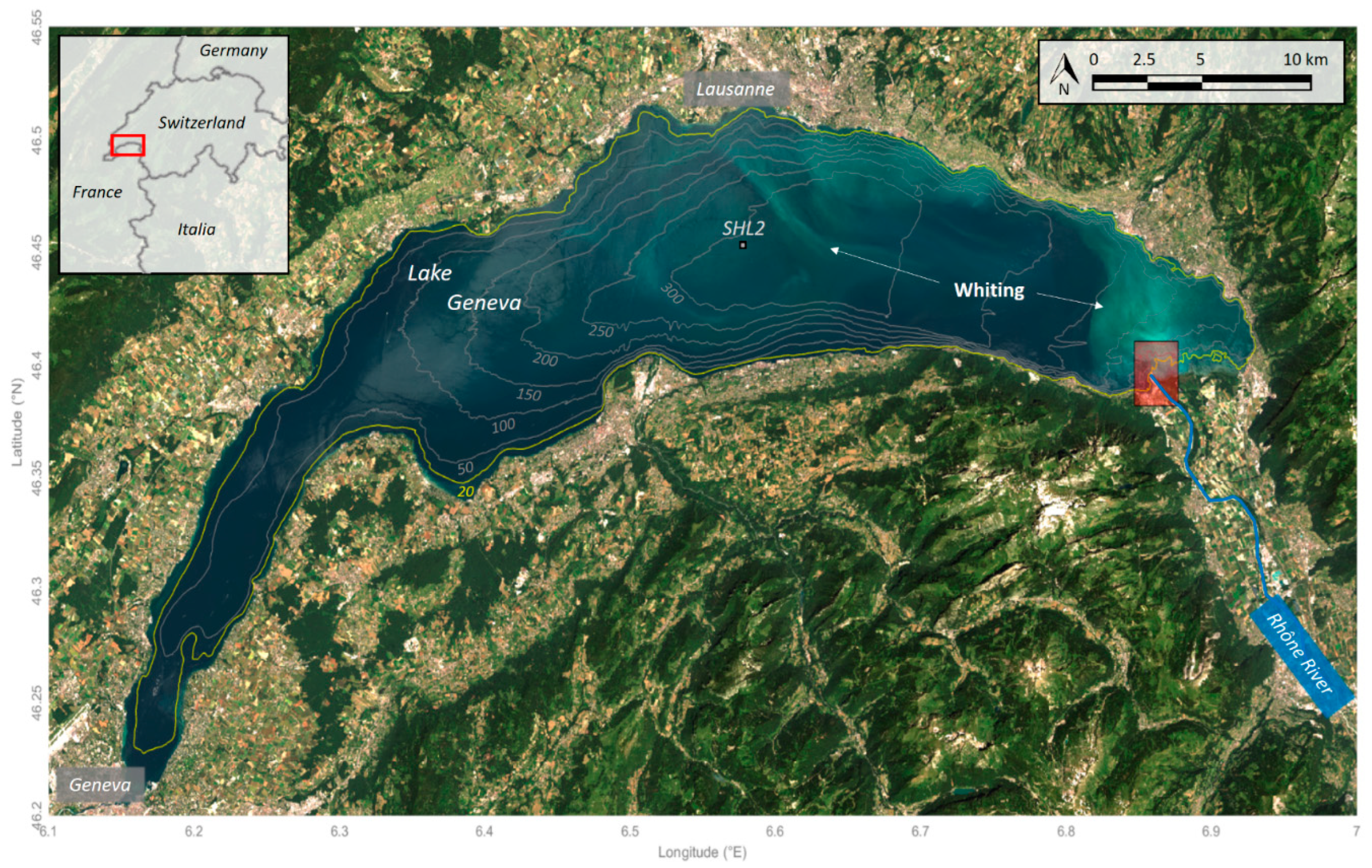
2. Study Site
3. Workflow and Data
3.1. Workflow
3.2. Satellite Data
3.3. Meteorological, Monitoring, and Climate Data
4. Methods
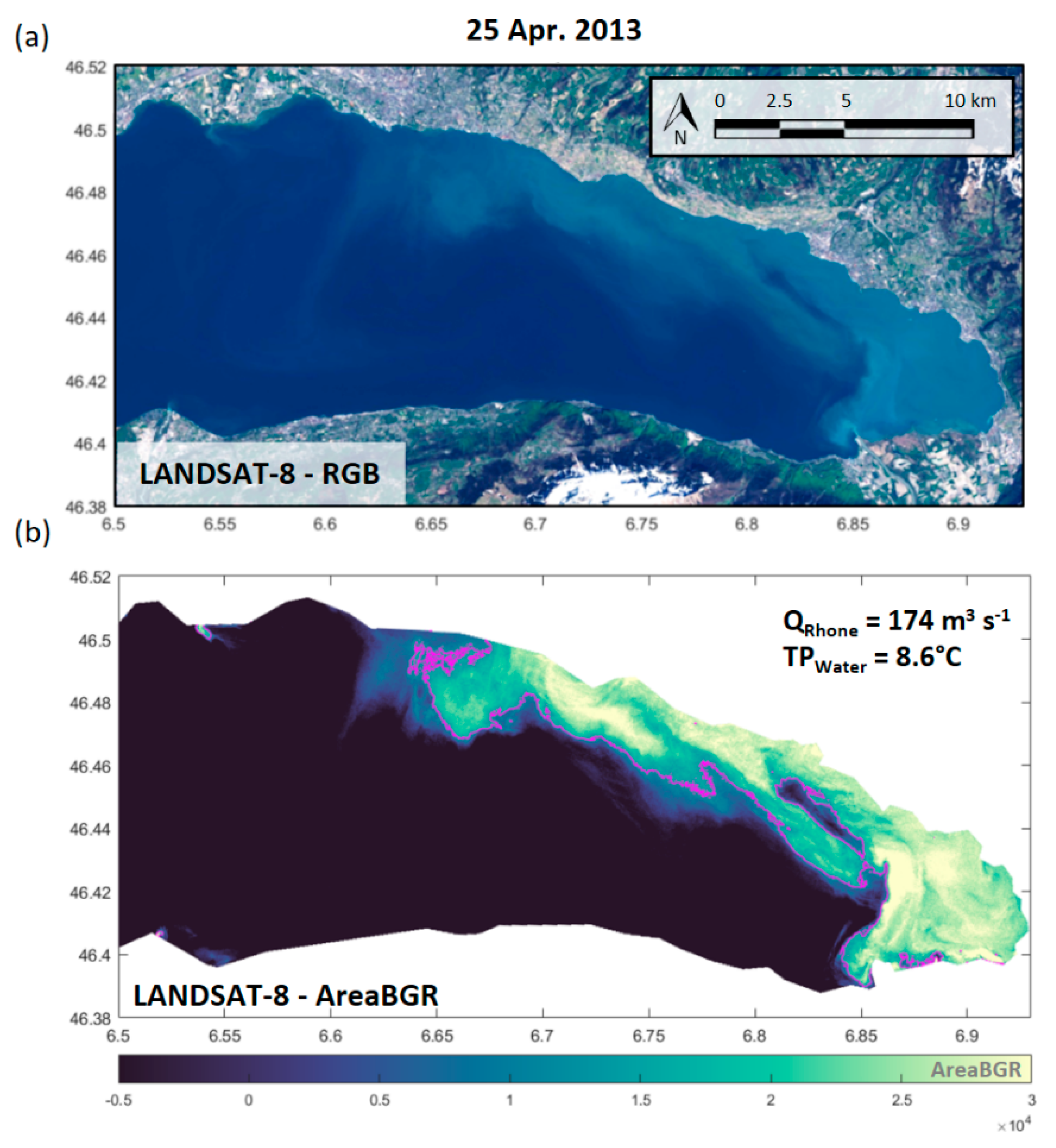
4.1. Whiting Detection Using Remote Sensing
4.2. Reconstruction of Past Whitings
5. Results
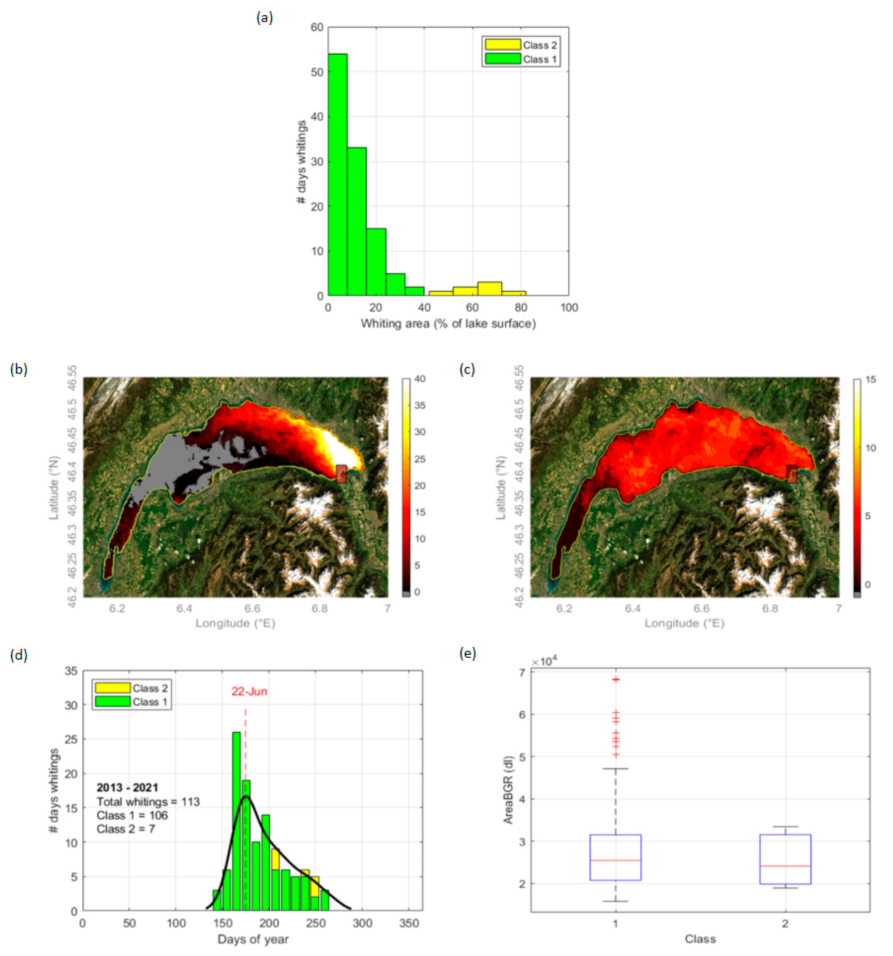
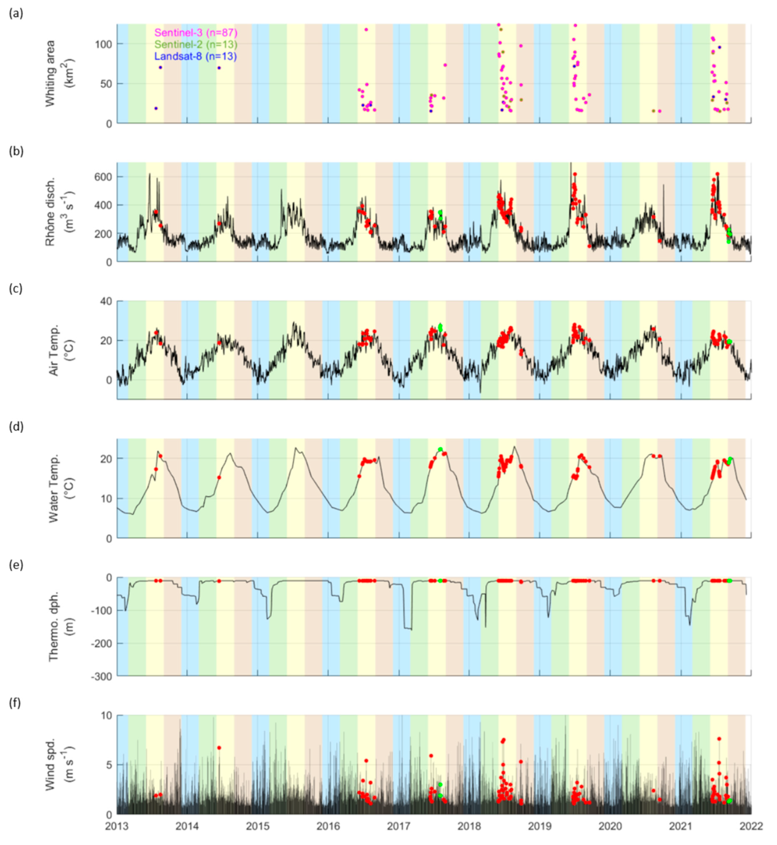
5.1. Spatial and Temporal Occurrences of Whitings in Lake Geneva from 2013 to 2021
5.1.1. Spatial Occurrences of Observed Whitings in Lake Geneva
5.1.2. Temporal Occurrences of Observed Whitings in Lake Geneva
5.2. Machine Learning and Statistical Approach
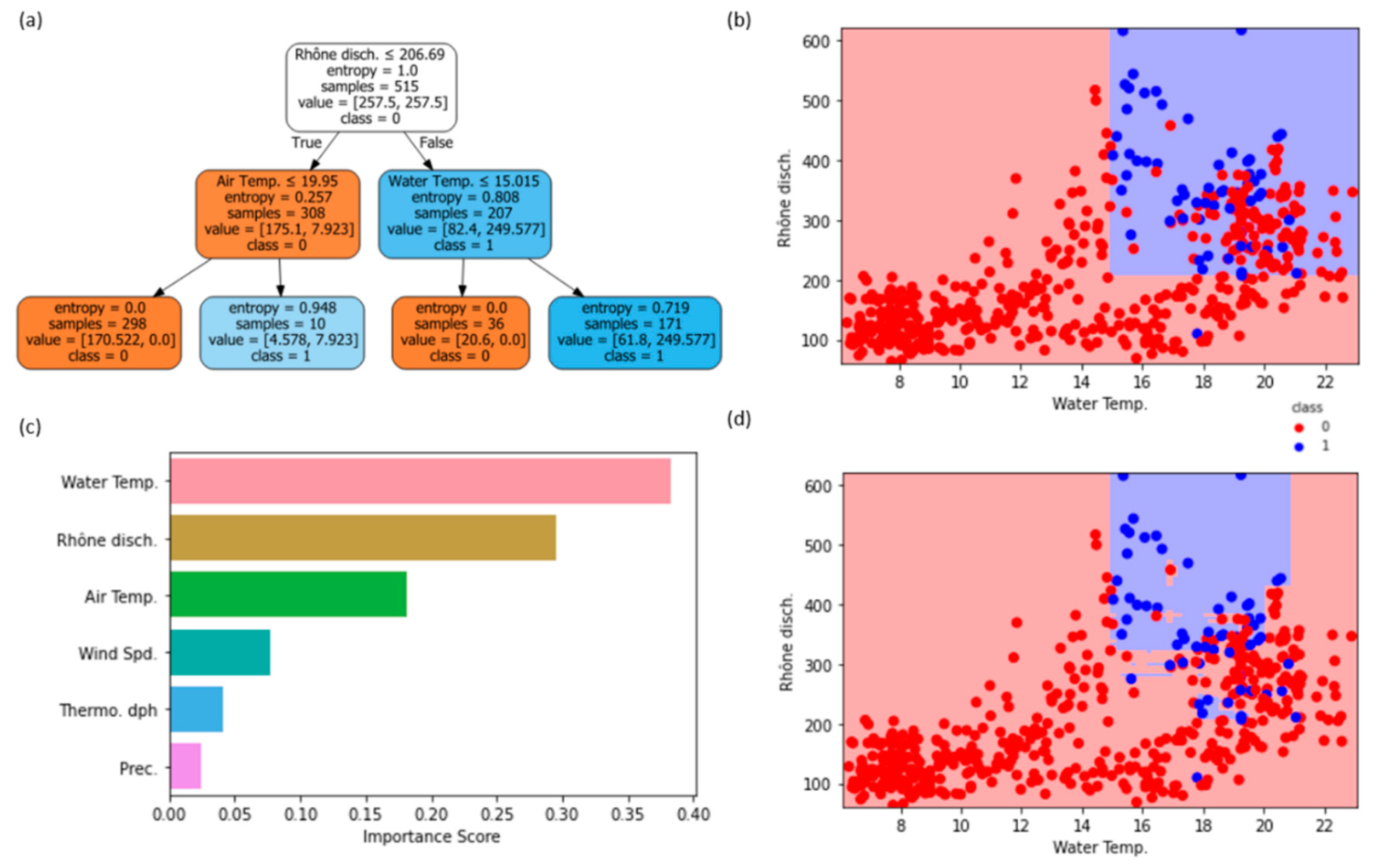
5.2.1. Drivers of Whitings Using Machine Learning
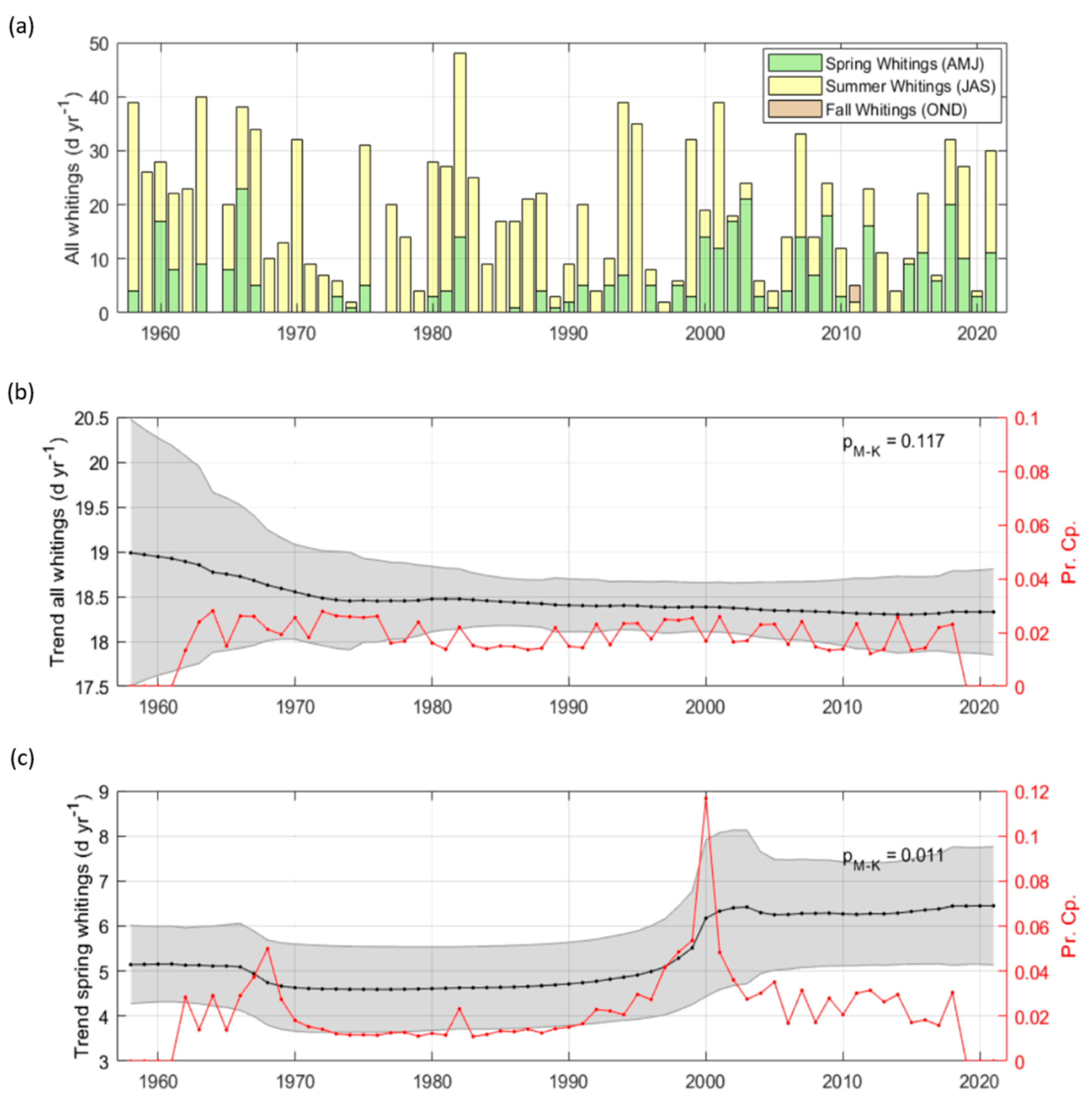
5.2.2. Reconstruction of Past Unseen Whitings
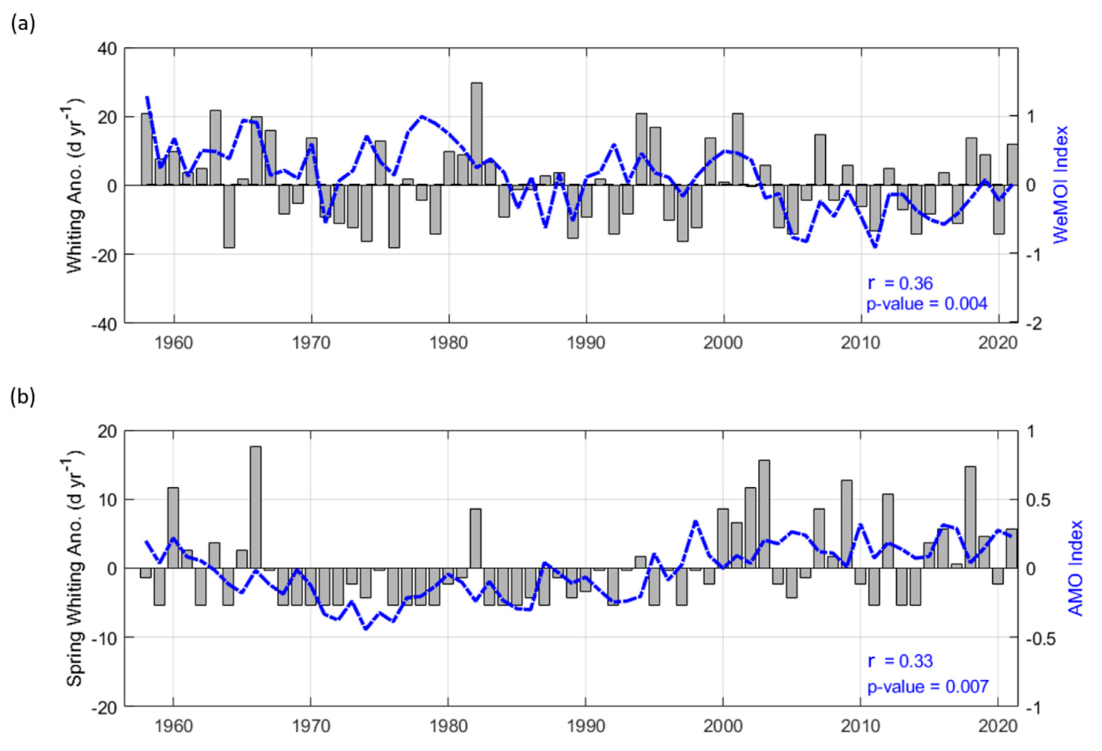
5.2.3. Factors Controlling Occurrences of Whitings from 1958 to 2021
6. Discussion
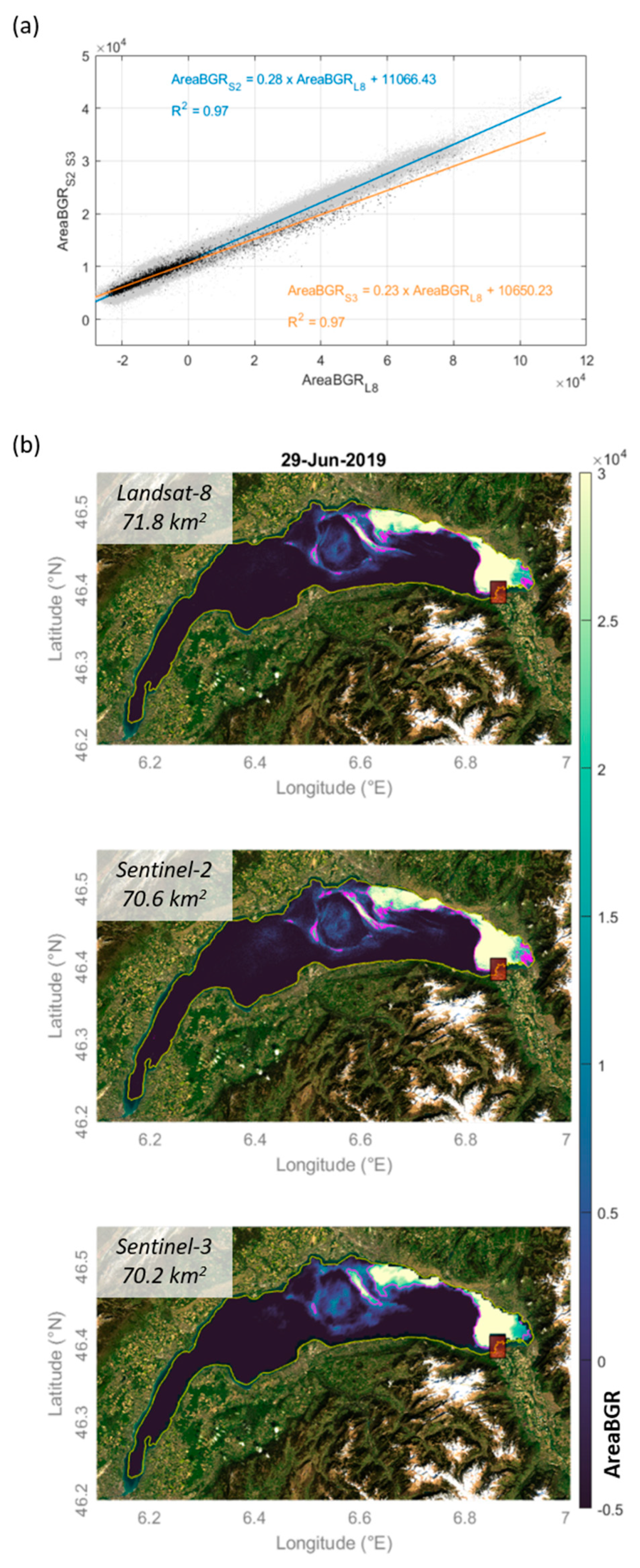
6.1. Remote Sensing of Whitings in Lake Geneva
6.2. Spatial and Temporal Occurrences of Whitings in Lake Geneva
6.3. The Long-Term Evolution of Whitings in Lake Geneva
7. Conclusions
Supplementary Materials
Author Contributions
Funding
Data Availability Statement
Acknowledgments
Conflicts of Interest
References
- Ridgwell, A.; Zeebe, R.E. The role of the global carbonate cycle in the regulation and evolution of the Earth system. Earth Planet. Sci. Lett. 2005, 234, 299–315. [Google Scholar] [CrossRef]
- Khan, H.; Marcé, R.; Laas, A.; Obrador Sala, B. The relevance of pelagic calcification in the global carbon budget of lakes and reservoirs. Limnetica 2022, 41. [Google Scholar] [CrossRef]
- Müller, B.; Meyer, J.S.; Gächter, R. Alkalinity regulation in calcium carbonate-buffered lakes. Limnol. Oceanogr. 2016, 61, 341–352. [Google Scholar] [CrossRef]
- Sondi, I.; Juracic, M. Whiting events and the formation of aragonite in Mediterranean Karstic Marine Lakes: New evidence on its biologically induced inorganic origin. Sedimentology 2010, 57, 85–95. [Google Scholar] [CrossRef]
- Larson, E.B.; Mylroie, J.E. A review of whiting formation in the Bahamas and new models. Carbonates Evaporites 2014, 29, 337–347. [Google Scholar] [CrossRef]
- Shanableh, A.; Al-Ruzouq, R.; Gibril MB, A.; Flesia, C.; Al-Mansoori, S. Spatiotemporal mapping and monitoring of whiting in the semi-enclosed gulf using moderate resolution imaging spectroradiometer (MODIS) time series images and a generic ensemble tree-based model. Remote Sens. 2019, 11, 1193. [Google Scholar] [CrossRef]
- Shanableh, A.; Al-Ruzouq, R.; Gibril MB, A.; Khalil, M.A.; AL-Mansoori, S.; Yilmaz, A.G.; Flesia, C. Potential Factors That Trigger the Suspension of Calcium Carbonate Sediments and Whiting in a Semi-enclosed Gulf. Remote Sens. 2021, 13, 4795. [Google Scholar] [CrossRef]
- Strong, A.E.; Eadie, B.J. Satellite observations of calcium carbonate precipitations in the Great Lakes 1. Limnol. Oceanogr. 1978, 23, 877–887. [Google Scholar] [CrossRef]
- Effler, S.W. The importance of whiting as a component of raw water turbidity. J. -Am. Water Work. Assoc. 1987, 79, 80–82. [Google Scholar] [CrossRef]
- Thompson, J.B.; Schultze-Lam, S.; Beveridge, T.J.; Des Marais, D.J. Whiting events: Biogenic origin due to the photosynthetic activity of cyanobacterial picoplankton. Limnol. Oceanogr. 1997, 42, 133–141. [Google Scholar] [PubMed]
- Nouchi, V.; Kutser, T.; Wüest, A.; Müller, B.; Odermatt, D.; Baracchini, T.; Bouffard, D. Resolving biogeochemical processes in lakes using remote sensing. Aquat. Sci. 2019, 81, 27. [Google Scholar] [CrossRef]
- Peng, F.; Effler, S.W. Characterizations of calcite particles and evaluations of their light scattering effects in lacustrine systems. Limnol. Oceanogr. 2017, 62, 645–664. [Google Scholar] [CrossRef]
- Hodell, D.A.; Schelske, C.L.; Fahnenstiel, G.L.; Robbins, L.L. Biologically induced calcite and its isotopic composition in Lake Ontario. Limnol. Oceanogr. 1998, 43, 187–199. [Google Scholar] [CrossRef]
- Stabel, H.H. Calcite precipitation in Lake Constance: Chemical equilibrium, sedimentation, and nucleation by algae 1. Limnol. Oceanogr. 1986, 31, 1081–1094. [Google Scholar] [CrossRef]
- Peng, F.; Effler, S.W. Characterizations of the light-scattering attributes of mineral particles in Lake Ontario and the effects of whiting. J. Great Lakes Res. 2011, 37, 672–682. [Google Scholar] [CrossRef]
- Effler, S.W.; Peng, F. Light-scattering components and Secchi depth implications in Onondaga Lake, New York, USA. Fundam. Appl. Limnol. 2012, 179, 251–265. [Google Scholar] [CrossRef]
- Escoffier, N.; Perolo, P.; Lambert, T.; Rüegg, J.; Odermatt, D.; Adatte, T.; Perga, M.E. Whiting events in a large peri-alpine lake: Evidence of a catchment-scale process. J. Geophys. Res. Biogeosci. 2022, 127, e2022JG006823. [Google Scholar] [CrossRef]
- Dierssen, H.M.; Zimmerman, R.C.; Burdige, D.J. Optics and remote sensing of Bahamian carbonate sediment whitings and potential relationship to wind-driven Langmuir circulation. Biogeosciences 2009, 6, 487–500. [Google Scholar] [CrossRef]
- Long, J.S.; Hu, C.; Robbins, L.L.; Byrne, R.H.; Paul, J.H.; Wolny, J.L. Optical and biochemical properties of a southwest Florida whiting event. Estuar. Coast. Shelf Sci. 2017, 196, 258–268. [Google Scholar] [CrossRef]
- Heine, I.; Brauer, A.; Heim, B.; Itzerott, S.; Kasprzak, P.; Kienel, U.; Kleinschmit, B. Monitoring of calcite precipitation in hardwater lakes with multi-spectral remote sensing archives. Water 2017, 9, 15. [Google Scholar] [CrossRef]
- Binding, C.E.; Greenberg, T.A.; Watson, S.B.; Rastin, S.; Gould, J. Long term water clarity changes in North America’s Great Lakes from multi-sensor satellite observations. Limnol. Oceanogr. 2015, 60, 1976–1995. [Google Scholar] [CrossRef]
- Long, J.S.; Hu, C.; Wang, M. Long-term spatiotemporal variability of southwest Florida whiting events from MODIS observations. Int. J. Remote Sens. 2018, 39, 906–923. [Google Scholar] [CrossRef]
- Schwefel, R.; Gaudard, A.; Wüest, A.; Bouffard, D. Effects of climate change on deepwater oxygen and winter mixing in a deep lake (Lake Geneva): Comparing observational findings and modeling. Water Resour. Res. 2016, 52, 8811–8826. [Google Scholar] [CrossRef]
- Molinero, J.C.; Anneville, O.; Souissi, S.; Lainé, L.; Gerdeaux, D. Decadal changes in water temperature and ecological time series in Lake Geneva, Europe—Relationship to subtropical Atlantic climate variability. Clim. Res. 2007, 34, 15–23. [Google Scholar] [CrossRef]
- Ottersen, G.; Planque, B.; Belgrano, A.; Post, E.; Reid, P.C.; Stenseth, N.C. Ecological effects of the North Atlantic oscillation. Oecologia 2001, 128, 1–14. [Google Scholar] [CrossRef] [PubMed]
- Loizeau, J.L.; Dominik, J. Evolution of the Upper Rhone River discharge and suspended sediment load during the last 80 years and some implications for Lake Geneva. Aquat. Sci. 2000, 62, 54–67. [Google Scholar] [CrossRef]
- Perga, M.E.; Maberly, S.C.; Jenny, J.P.; Alric, B.; Pignol, C.; Naffrechoux, E. A century of human-driven changes in the carbon dioxide concentration of lakes. Glob. Biogeochem. Cycles 2016, 30, 93–104. [Google Scholar] [CrossRef]
- Lambert, T.; Perga, M.E. Non-conservative patterns of dissolved organic matter degradation when and where lake water mixes. Aquat. Sci. 2019, 81, 64. [Google Scholar] [CrossRef]
- Giovanoli, F. Horizontal transport and sedimentation by interflows and turbidity currents in Lake Geneva. In Large Lakes; Springer: Berlin/Heidelberg, Germany, 1990; pp. 175–195. [Google Scholar]
- Kumar, L.; Mutanga, O. Google Earth Engine applications since inception: Usage, trends, and potential. Remote Sens. 2018, 10, 1509. [Google Scholar] [CrossRef]
- Mutanga, O.; Kumar, L. Google earth engine applications. Remote Sens. 2019, 11, 591. [Google Scholar] [CrossRef]
- Wulder, M.A.; Loveland, T.R.; Roy, D.P.; Crawford, C.J.; Masek, J.G.; Woodcock, C.E.; Zhu, Z. Current status of Landsat program, science, and applications. Remote Sens. Environ. 2019, 225, 127–147. [Google Scholar] [CrossRef]
- Muller-Wilm, U.; Louis, J.; Richter, R.; Gascon, F.; Niezette, M. Sentinel-2 level 2A prototype processor: Architecture, algorithms and first results. In Proceedings of the ESA Living Planet Symposium, Edinburgh, UK, 9–13 September 2013; pp. 9–13. [Google Scholar]
- Steinmetz, F.; Ramon, D. Sentinel-2 MSI and Sentinel-3 OLCI consistent ocean colour products using POLYMER. In Remote Sensing of the Open and Coastal Ocean and Inland Waters; SPIE: Honolulu, HI, USA, 2018; Volume 10778, pp. 46–55. [Google Scholar]
- Copernicus. Copernicus Global Land Operations “Cryosphere and Water” “CGLOPS-2”—Algorithm Theoretical Basis Document Lake Waters 300m and 1km Products Versions 1.3.0-1.4.0 Issue I1.12. 2020. Available online: https://land.copernicus.eu/global/sites/cgls.vito.be/files/products/CGLOPS2_PUM_LWQ300_1km_v1.3.1_I1.10.pdf (accessed on 23 October 2022).
- ESA. D2.2: Algorithm Theoretical Basis Document. 2020. Available online: https://climate.esa.int/media/documents/CCI-LAKES-0024-ATBD-v2.3.pdf (accessed on 23 October 2022).
- Rimet, F.; Anneville, O.; Barbet, D.; Chardon, C.; Crepin, L.; Domaizon, I.; Monet, G. The Observatory on LAkes (OLA) database: Sixty years of environmental data accessible to the public. J. Limnol. 2020, 79, 164–178. [Google Scholar] [CrossRef]
- FOEN. Commander des Données Hydrologiques Historiques et Validées. 2022. Available online: https://www.bafu.admin.ch/bafu/fr/home/themes/eaux/etat/donnees/obtenir-des-donnees-mesurees-sur-le-theme-de-l-eau/commander-des-donnees-hydrologiques-historiques-et-validees.html (accessed on 23 October 2022).
- Izquierdo Miguel, R.; Alarcón Jordán, M.; Avila Castells, A. WeMO effects on the amount and the chemistry of winter precipitation in the north-eastern Iberian Peninsula. Tethys J. Mediterr. Meteorol. Climatol. 2014, 10, 45–51. [Google Scholar] [CrossRef]
- Martin-Vide, J.; Lopez-Bustins, J.A. The western Mediterranean oscillation and rainfall in the Iberian Peninsula. Int. J. Climatol. A J. R. Meteorol. Soc. 2006, 26, 1455–1475. [Google Scholar] [CrossRef]
- McPhaden, M.J.; Zebiak, S.E.; Glantz, M.H. ENSO as an integrating concept in earth science. science 2006, 314, 1740–1745. [Google Scholar] [CrossRef] [PubMed]
- Lloyd-Hughes, B.; Saunders, M.A. Seasonal prediction of European spring precipitation from El Niño–Southern Oscillation and local sea-surface temperatures. Int. J. Climatol. A J. R. Meteorol. Soc. 2002, 22, 1–14. [Google Scholar] [CrossRef]
- Hastie, T.; Tibshirani, R.; Friedman, J.H.; Friedman, J.H. The Elements of Statistical Learning: Data Mining, Inference, and Prediction; Springer: New York, NY, USA, 2009; Volume 2, pp. 1–758. [Google Scholar]
- Géron, A. Hands-On Machine Learning with Scikit-Learn, Keras, and TensorFlow: Concepts, Tools, and Techniques to Build Intelligent Systems; O’Reilly Media, Inc.: Newton, MA, USA, 2019. [Google Scholar]
- Mann, H.B. Nonparametric tests against trend. Econom. J. Econom. Soc. 1945, 13, 245–259. [Google Scholar] [CrossRef]
- Kendall, M.G. Rank Correlation Methods; Griffin: Oxford, UK, 1948. [Google Scholar]
- Zhao, K.; Wulder, M.A.; Hu, T.; Bright, R.; Wu, Q.; Qin, H.; Brown, M. Detecting change-point, trend, and seasonality in satellite time series data to track abrupt changes and nonlinear dynamics: A Bayesian ensemble algorithm. Remote Sens. Environ. 2019, 232, 111181. [Google Scholar] [CrossRef]
- Verpoorter, C.; Kutser, T.; Seekell, D.A.; Tranvik, L.J. A global inventory of lakes based on high-resolution satellite imagery. Geophys. Res. Lett. 2014, 41, 6396–6402. [Google Scholar] [CrossRef]
- Spyrakos, E.; Hunter, P.; Simis, S.; Neil, C.; Riddick, C.; Wang, S.; Tyler, A. Moving towards global satellite based products for monitoring of inland and coastal waters. Regional examples from Europe and South America. In Proceedings of the 2020 IEEE Latin American GRSS & ISPRS Remote Sensing Conference (LAGIRS), Santiago, Chile, 22–26 March 2020; pp. 363–368. [Google Scholar]
- Seegers, B.N.; Werdell, P.J.; Vandermeulen, R.A.; Salls, W.; Stumpf, R.P.; Schaeffer, B.A.; Loftin, K.A. Satellites for long-term monitoring of inland US lakes: The MERIS time series and application for chlorophyll-a. Remote Sens. Environ. 2021, 266, 112685. [Google Scholar] [CrossRef] [PubMed]
- Cotte, G.; Vennemann, T.W. Mixing of Rhône River water in Lake Geneva: Seasonal tracing using stable isotope composition of water. J. Great Lakes Res. 2020, 46, 839–849. [Google Scholar] [CrossRef]
- CIPEL Report. Available online: https://www.cipel.org/wp-content/uploads/catalogue/rs-camp-2017-03phytoplancton-v1.pdf (accessed on 23 October 2022).
- UMR CARRTEL INRAE USMB. Bienvenue à l’UMR CARRTEL. Bloom d’une Microalgue, sur le Léman: Uroglena sp. Non Toxique, qui Colore l’eau en Marron. inra.com. 2021. Available online: https://www6.lyon-grenoble.inrae.fr/carrtel_fre/Centre-Alpin-de-Recherche-sur-les-Reseaux-Trophiques-des-Ecosystemes-Limniques/Actualites-CARRTEL-INRAE-USMB/Bloom-d-une-microalgue-sur-le-Leman-Uroglena-sp.-non-toxique-qui-colore-l-eau-en-marron (accessed on 23 October 2022).
- Dittrich, M.; Obst, M. Are picoplankton responsible for calcite precipitation in lakes? AMBIO A J. Hum. Environ. 2004, 33, 559–564. [Google Scholar] [CrossRef] [PubMed]
- Knight, J.R.; Folland, C.K.; Scaife, A.A. Climate impacts of the Atlantic multidecadal oscillation. Geophys. Res. Lett. 2006, 33, L17706. [Google Scholar] [CrossRef]
- Zobrist, J.; Schoenenberger, U.; Figura, S.; Hug, S.J. Long-term trends in Swiss rivers sampled continuously over 39 years reflect changes in geochemical processes and pollution. Environ. Sci. Pollut. Res. 2018, 25, 16788–16809. [Google Scholar] [CrossRef] [PubMed]
- Lane, S.N.; Bakker, M.; Costa, A.; Girardclos, S.; Loizeau, J.L.; Molnar, P.; Schlunegger, F. Making stratigraphy in the Anthropocene: Climate change impacts and economic conditions controlling the supply of sediment to Lake Geneva. Sci. Rep. 2019, 9, 8904. [Google Scholar] [CrossRef]
- Freudiger, D.; Vis, M.; Seibert, J. Quantifying the Contributions to Discharge of Snow and Glacier Melt; Hydro-CH2018 Project; Commissioned by the Federal Office for the Environment (FOEN): Bern, Switzerland, 2020; 49p. [Google Scholar]


| Sensor | OLI | MSI | OLCI |
|---|---|---|---|
| Spatial resolution (m) | 30 | 10−60 ** | 300 |
| Swath width (km) | 180 | 290 | 1270 |
| Temporal resolution * (days) | 16 | 5 | 1 |
| Available period | 2013−2021 | 2017−2021 | 2016−2021 |
| λblue | 480 | 490 | 490 |
| λgreen | 560 | 560 | 560 |
| λref | 655 | 665 | 665 |
| Cloud−free images used | 140 | 101 | 766 |
| Parameter (Unit) | Class 1 (Mean +/− Std.) | Class 2 (Mean +/− Std.) |
|---|---|---|
| Rhone discharge (m3 s−1) | 363.1 +/− 102.9 | 251.1 +/− 81.4 |
| Air temperature (°C) | 21.5 +/− 3.0 | 22.3 +/− 3.8 |
| Surface water temperature (°C) | 17.9 +/− 1.8 | 20.6 +/− 1.7 |
| Wind speed (m s−1) | 2.4 +/− 1.4 | 1.7 +/− 0.6 |
| Thermocline depth (m) | 11.1 +/− 0.6 | 11.0 +/− 0.0 |
| Number of obs. days | 106 | 7 |
Publisher’s Note: MDPI stays neutral with regard to jurisdictional claims in published maps and institutional affiliations. |
© 2022 by the authors. Licensee MDPI, Basel, Switzerland. This article is an open access article distributed under the terms and conditions of the Creative Commons Attribution (CC BY) license (https://creativecommons.org/licenses/by/4.0/).
Share and Cite
Many, G.; Escoffier, N.; Ferrari, M.; Jacquet, P.; Odermatt, D.; Mariethoz, G.; Perolo, P.; Perga, M.-E. Long-Term Spatiotemporal Variability of Whitings in Lake Geneva from Multispectral Remote Sensing and Machine Learning. Remote Sens. 2022, 14, 6175. https://doi.org/10.3390/rs14236175
Many G, Escoffier N, Ferrari M, Jacquet P, Odermatt D, Mariethoz G, Perolo P, Perga M-E. Long-Term Spatiotemporal Variability of Whitings in Lake Geneva from Multispectral Remote Sensing and Machine Learning. Remote Sensing. 2022; 14(23):6175. https://doi.org/10.3390/rs14236175
Chicago/Turabian StyleMany, Gaël, Nicolas Escoffier, Michele Ferrari, Philippe Jacquet, Daniel Odermatt, Gregoire Mariethoz, Pascal Perolo, and Marie-Elodie Perga. 2022. "Long-Term Spatiotemporal Variability of Whitings in Lake Geneva from Multispectral Remote Sensing and Machine Learning" Remote Sensing 14, no. 23: 6175. https://doi.org/10.3390/rs14236175
APA StyleMany, G., Escoffier, N., Ferrari, M., Jacquet, P., Odermatt, D., Mariethoz, G., Perolo, P., & Perga, M.-E. (2022). Long-Term Spatiotemporal Variability of Whitings in Lake Geneva from Multispectral Remote Sensing and Machine Learning. Remote Sensing, 14(23), 6175. https://doi.org/10.3390/rs14236175