Abstract
Morphometric studies of scoria cones have a long history in research. Their geometry and shape are believed to be related to evolution by erosion after their formation, and hence the morphometric parameters are supposed to be related with age. We analysed 501 scoria cones of four volcanic fields: San Francisco Volcanic Field (Arizona, USA), Chaîne des Puys (France), Sierra Chichinautzin (Mexico), and Kula Volcanic Field (Turkey). All morphometric parameters (cone height, cone width, crater width, slope angles, ellipticity) were derived using DTMs. As new parameters, we calculated Polar Coordinate Transformed maps, Spatial Elliptical Fourier Descriptors to study the asymmetries. The age groups of the four volcanic fields were created and their slope distributions were analysed. The age groups of individual volcanic fields show a statistically significant decreasing tendency of slope angles tested by Mann–Whitney tests. By mixing the age groups of the volcanic fields and sorting them by age interval, we can also observe a general, statistically significant decrease. The interquartile ranges of the distributions also tend to decrease with time. These observations support the hypothesis that whereas the geometry of individual scoria cones differs initially (just after formation), general trends may exist for their morphological evolution with time in the various volcanic fields.
1. Introduction
Scoria cones are arguably the simplest and most common volcanic landforms. Even if they are created by various eruptive styles (low-explosivity Hawaiian or Strombolian eruptions or, rarely, by violent Strombolian or phreatomagmatic activity), their shape tends to follow a regular geometry (see later). Hence, their shape can be parameterized mathematically relatively easily, which has allowed researchers to conduct detailed geomorphometry analysis [1,2]. However, the precision of early work in the second half of the 20th century (a brief summary is given below) was greatly limited due to the low resolution of contour maps and required tedious manual outlining and/or measurements on printed maps. The increasing availability of digital elevation data and the advent of new imaging technology allow researchers to perform these geomorphometric tasks using GIS (Geographic Information Systems). New processing tools have emerged; various surface analysis modules and plug-ins are becoming increasingly common in GIS software. These have recently made mapping and analysing different landforms and developing new methods one of the most dynamically evolving fields of geomorphometry. The combination of elevation models and appropriate software allows the (semi)automated processing of areas that would be otherwise difficult to process with classical surveying; large areas can be processed cost-effectively, quickly, and objectively.
One advantage of this standardisation is the ability of comparing measurements made in different volcanic areas. The present study yields this example. Once the parameters have been calculated, we can compare the parameter distributions of the volcanic areas. This study has been performed on a test basis to verify if geometry can be seen to vary with age over different volcanic fields with this new approach.
In the previous studies (a concise review is given in the next section), the focus was on the parameterization of the individual cones in order to relate them to their age. This effort was sometimes successful, but the wide variety of cone geometries often blurs this relationship. Some years ago, we also followed this principle [3,4]; however, our findings show distributional overlaps. Therefore, we changed our approach to study the distributions of the parameters of the cones instead [5]; this gives a more robust result in many cases. The important research question in this case is: is it possible to form non-overlapping age groups of cones so that even if their parameter (e.g., slope) distributions are overlapping, the statistical test applied to their distributions finds a significant difference? Our answer is yes, if the slope values are determined using a high-resolution digital terrain model. In the current study we took another step ahead. We compared the distributions of four different volcanic areas (where high-resolution DTMs and age data were available) to test whether such a comparison makes sense or not.
In theory, all scoria cone fields can be used for comparison. The volcanic areas (San Francisco Volcanic Field, Arizona, USA; Chaîne des Puys, France; Sierra Chichinautzin, Mexico; and Kula Volcanic Field, Turkey) were selected for this purpose because (1) there was high-resolution DTM available, so that the morphometric calculation could be performed with high accuracy, and (2) we had access to good quality age data. Concerning the age data, there was another advantage (except for Chaîne des Puys). The age grouping had already been performed by previous authors (see geological background and references in the next section); this circumstance may increase the robustness of the grouping. Being at least successful in that, after this step, further research will be needed to establish robust comparison techniques and to reveal possible correlations that we consider as indications only in the present study.
The structure of our paper is as follows. In order to provide a proper overview of research in this field, in Section 2 the theoretical background is established including (1) a concise review of the previous morphometric approaches, and (2) a brief geological setting description of the four areas. In Section 3 the input data (DTMs) are specified, and the calculation methods of the classic and new morphometric parameters are described. Section 4 summarizes the results, including the visualizations of the parameter distributions, tabular results of the Mann–Whitney statistical tests, and examples of polar coordinate transformed images. In the discussion (Section 5) we consider the merged data set in statistical sense, highlighting the trends found in the data. Finally, in Section 6 we draw three important conclusions based on our findings.
2. Theoretical Background
2.1. Geomorphometry of Scoria Cones—Previous Research
The classic studies of monogenetic cones adopted a simple geometrical model of fresh scoria cones [6] and, for simplicity, did not consider any deformation, e.g., elongated, rifted, collapsed, or craterless cones. Although various types of cone asymmetry are common in many volcanic fields, in order to avoid undue complexity as a first stage, research focused chiefly on describing fairly regular cones. Consequently, only a few descriptive parameters were introduced in the first decades of morphometric studies. These techniques are briefly reviewed below.
2.1.1. Based on Classical (Field) Surveys
One of the earliest studies is Colton’s classic account of the morphology of the San Francisco Volcanic Field scoria cones in Arizona [7]. He classified the cones and basalt flows into five degradation stages based on successive erosion, as did Kear for the larger (complex) New Zealand volcanoes [8]. The Paricutín cone (Michoacán–Guanajuato Volcanic Field, Mexico), which erupted in 1943–1952, has also been the subject of numerous studies; those on the erosional processes and their rates were reported by Segerstrom [9,10,11]. Bloomfield studied the morphology, morphometry, chemistry, and radiometry of cones and lava flows in the Chichinautzin Volcanic Field in central Mexico [12]. Scott and Trask did the same for the Lunar Crater volcanic field in Nevada. They derived relative morphological ages for 15 cones using maximum cone slope and cone width/height ratios [13]. Settle investigated parameters including mean volume (V), cone height (Hco, see below), and diameter (Wco) for six volcanic fields (Mauna Kea, Hawaii, Mount Etna, Italy, Kilimanjaro, Tanzania, San Francisco Volcanic Field, Arizona, Paricutín, Mexico, Nunivak Island, Alaska) [14].
Porter was the first to establish the quantitative relationships of the morphology of cones. In his research, he investigated more than 300 cones on the upper slopes of Mauna Kea for degradation and asymmetry. He identified important volcanic parameter relationships that have been extensively used in comparative analyses. The following parameters of the scoria cones were investigated (and notation introduced, which is now de facto standard): crater width (Wcr), crater depth (Dcr), cone height (Hco), base width (Wco), and slope angle (α) (Figure 1).
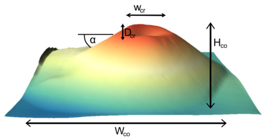
Figure 1.
Classic morphometric parameters of a scoria cone: crater width (Wcr), crater depth (Dcr), cone height (Hco), base width (Wco), and slope angle (α).
Wood followed this logic and made a morphometric analysis with the above parameters (and their further consideration) [2]. His work can be divided into two parts: first he analysed and compared the cones of the well-studied San Francisco Volcanic Field according to the age groups classified by Colton, and Moore et al. [7,15], and found clear evolutionary trends of shape parameters with age. Then, he investigated if the same trends were observed in five other scoria cones. He pointed out that large-scale topographic maps are not sufficiently precise to measure certain parameters (e.g., crater diameter).
2.1.2. DTM-Based Research
The first significant publication on scoria cone morphometry using the digital terrain model (DTM) for calculations was published in 1998 [16]. The authors not only drew various conclusions based on their field experience and from available geological/morphological maps, but also used a numerical approach to help study the changing morphology of the volcanic forms. In addition to the already examined San Francisco Volcanic Field, that study also focused on the scoria cones of the Springerville Volcanic Area, also in Arizona. The morphology and morphometry were determined from topographic maps, field surveys, field photographs, and aerial photographs. The maximum slope angle values were calculated from field surveys, aerial photographs, and the distance between contour lines. To supplement these data, DTMs from the United States Geological Survey were used.
The relationships published in the studies presented so far are mainly ideal for regular, circular, or elliptical cones. For irregular cones, a more advanced geometric description was needed, and the diameter definition for irregular cones was of great importance. In contrast to previous studies that concentrated on scoria cones deposited on a (sub)horizontal plane, Favalli et al. studied examples that were emplaced on the steep slopes of Etna, using a higher resolution (2 m) DTM [17]. For a tilted base ground, the calculation of the original cone parameters had to be changed; the values had to be projected into a 2D plane.
This logic was followed by Fornaciai et al. [18]. In their work, freely available DEMs were used, and 21 volcanic areas with different locations, climates, and numbers of volcanic units were investigated. They pointed out that an important consideration in the selection of scoria cone areas is the resolution of the DEM available for the area. They did not recommend the 90 m SRTM (Shuttle Radar Topography Mission), while they did recommend the 30 m ASTER (Advanced Spaceborne Thermal Emission and Reflection Radiometer) and better resolution data (e.g., Lidar). Fornaciai et al. also studied the minor but possibly systematic variability of scoria cone morphology constrained by the tectonic setting, and also the shape modification due to long-term erosion. Extinct scoria cones display a progressive change in terms of morphometry (e.g., Hco/Wco), which is related to the variations of eruptive style, lithology, and climate [8,9,17,18,19].
Summing up the results related to resolution, the 10 m resolution DTM was also preferred (if available) but it also had an error of over 10% for small cones. In total, morphometric parameters (V, slope, Hco, Wco, and Wcr) and geometric ratios (Hco/Wco and Wcr/Wco) were calculated for 542 cones. Vörös et al. [19] also examined the differences resulting from the resolution, highlighting the importance of a properly selected resolution in the case of slope angle calculations.
2.2. Study Areas and Age Groups
2.2.1. Chaîne des Puys (CdP)
The Chaîne des Puys is a 25 km long, complex, closely spaced lineament of 80 volcanoes in the Massif Central of France. The oldest cones are up to about 95,000 years old, the age of the youngest only about 9000 years. The volcanoes generally are located less than 1 km apart, and because of this close proximity have tended to erupt their material onto the margin of their neighbours. The top layer, thus, in older volcanoes actually can overlap with one or more of the other younger cones. The composition of the erupted magmas ranges from basalt to trachyte. The more evolved ones mostly form domes and spines, while the basalt to trachyandesite compositions form scoria cones. The cones and domes have very diverse morphology, ranging from simple cones with craters, through breached or open cones, to multiple vent cones, and ones deformed by magma intruding beneath. Their aprons are also highly diverse.
The Chaîne des Puys lineament is set in a much wider volcanic field, active for at least 20 million years, with thousands of scoria cones, and some associated larger centres (the Mont Dore and Sancy stratovolcanoes). The older scoria cones are extensively degraded due to high erosion rates related to regional uplift in the Quaternary.
For this volcanic area, age groups have not been created before. Due to the statistical test presented in Section 2.2.2, the cones between 8 and 64 thousand years were divided into three groups in such a way that each one had (almost) the same number of cones. Thus, there are 9-8-9 cones in each established age group (Figure 2).
2.2.2. San Francisco Volcanic Field (SFVF)
The San Francisco Volcanic Field is located near the city of Flagstaff, Arizona (USA) in the southern Colorado Plateau. The whole area covers roughly 4700 km2, with about 600 scoria cones, lava domes, lava flows, and extensive scoria and ash deposits [20]. Several similar volcanic areas have formed on the North American continent since the Neogene, but the largest, most productive eruptions are associated with the southern part of the plateau. These large—mostly basaltic—volcanic areas bisect Arizona along a southeast–northwest axis. In addition to the San Francisco Volcanic Field, Mormon or Springerville volcanic areas have comparable character [21]. They have formed in a similar way, from the late Miocene onwards; this part of the North American plate suffered delamination (the lower lithosphere detached and sank), and the crust thinned and became uplifted as the aesthenosphere rose and melted to produce the magmas [22]. The dominant lithology is alkali basalt. In addition to basalt, andesite is also found; andesite is the dominant rock of the San Francisco stratovolcano, the central landform of the area [23]. Some volcanoes of this field have higher SiO2 content, higher-viscosity dacites or even rhyolitic composition [24]. The volcanic history here dates back only 5–6 million years. Within this interval, the age of the structures ranges widely. Some are just a few thousand years old (Sunset Crater), others 1 million years old (San Francisco Mountain: 0.4–1 million years) to several millions of years old (Bill Williams Mountain: 5–6 million years) [25].
The older Pliocene scoria cones are found in the western and south-western parts of the San Francisco Field, while in the eastern part, a younger trend is observed [25]. The easternmost cones are of the Late Pleistocene–Holocene age. This rejuvenating trend may be evidence that the area was formed over a hotspot [20]. Based on Colton [7], Moore and Wolfe [15], and USGS 1: 50,000 maps, five age groups were created (see in Figure 2b).
2.2.3. Sierra Chichinautzin (SC)
The Sierra Chichinautzin is located south of Mexico City, in the central-eastern part of the Trans-Mexican Volcanic Belt, a ca. 1000 km-long active continental arc related to a subduction zone. The volcanic field covers an area of ca. 2500 km2 with >300 edifices, most of which are scoria cones with lavas, with a few medium-sized shields and thick lava flows and domes (e.g., [12,26,27,28,29,30,31]). The dominant rock composition is calc-alkaline andesite, with some trachybasalts and dacites [32,33].
The age of the volcanoes ranges from Holocene, with the Xitle volcano being the youngest dated volcano at ca. 1670 yr BP [34] to 1.2 Ma for a deeply eroded cone at the foot of the Nevado de Toluca volcano [35]. Vásquez [36] classified the scoria cones into three age groups (Figure 2), based on available age data [27,28,30,31,34,35,37] and the stage of degradation of the cones (depth and spatial frequency of gullies on external slopes, filling of the crater). Note that Lidar-based topographical data are available only for the central and eastern parts of the field, hence the only parts investigated in this study.
2.2.4. Kula Volcanic Field (KVF)
The Kula volcanic field is located in western Turkey, in western Anatolia, one of the most rapidly extending regions on Earth at a rate of ~20 mm/year [38,39]. This volcanic province is one of Turkey’s youngest volcanic fields, remains active throughout the Quaternary, and is located on a horst system at an elevation range of 500 to 1054 m (a.s.l.).
The volcanic evolution of the Kula has been divided into three explosive and effusive eruption phases: Stage-IV Basalts (β2 (ca. 2–1 Ma)), Stage-III Basalts (β3 (ca. 300–50 ka)), and the youngest one, Stage-II Basalt (β4 (<25 ka)) [40,41,42,43,44,45,46]. The field covers an area of ~350 km2 with >80 edifices, most of which are scoria cones with lavas and maars and spatter cones of different areal extent. The volume of Kula basaltic lavas was estimated to be approximately 2.3 km3 [47]. The total dense rock equivalent (DRE) volume of volcanic products, including lava flows and pyroclastics (scoria cones, maars, and tephra), is calculated to be ~5.9 km3 [48]. Based on their chemical compositions, the volcanic products have an alkaline character and are classified as basanite and phonotephrite [49]. Clinopyroxene, olivine, hornblende (for β2 and β3 stage), plagioclase, and feldspathoids dominate the mineral assemblage in basaltic lavas [49].

Figure 2.
(a) Location and (b) age scales and groups of the examined four volcanic areas.
3. Materials and Methods
3.1. Use of DTMs
Based on previous studies [17,18], the selection of a DTM with appropriate resolution is a key issue. Today global databases are available in a moderately high resolution (e.g., ~10–30 m), and the local/regional sources can even exceed this. Although our basic goal was to use DTMs with the best possible resolution, we also aimed to create a processing algorithm that could be used for as many different databases as possible. That is why we worked with DTMs of various resolutions, but the lowest resolution was below 15 m.
3.1.1. Chaîne des Puys
Among the four areas, on average, the Chaîne des Puys area has the best resolution LIDAR terrain model courtesy of CRAIG (Centre Regional de Informational Geographique [50]. The central part of the chain is accessible in 0.5 m resolution while the whole Clermont Auvergne Metropolitan area is covered with a 5 m LIDAR set [51]. The dataset can be downloaded from CRAIG.
3.1.2. San Francisco Volcanic Field
Various DTMs are available in the United States of America. Most of them can be downloaded free of charge from the USGS (United States Geological Survey) website [52]. The DTMS are primarily derived from topographic maps, but they are increasingly taken over/supplemented with Lidar measurements these days. The 1 m DEMs of the 3D Elevation Program (3DEP) is one of the Lidar-based projects [53]. Unfortunately, it is not yet available for the entire area investigated, so in some cases, the 10 m (1/3 arc-second) terrain model was used [54].
3.1.3. Sierra Chichinautzin
Lidar-based DTM with horizontal resolution of 5 m and vertical resolution of 1 m, available from the website of the Instituto Nacional de Estadística y Geografía (INEGI-[55]).
3.1.4. Kula Volcanic Field
TanDEM-X (TerraSAR-X add-on for Digital Elevation Measurements) is an Earth observation radar mission based on utilizing the two Xband radar satellites TerraSAR-X and TanDEM-X flying in a helix-like formation. The TanDEM-X DEM has a planar resolution of 12 m, with a relative vertical accuracy of 2 m, and absolute vertical accuracy of 10 m for a 90% confidence interval. In this study, the available data for Kula were resampled to 12.5 m for noise reduction.
In general, the resolutions of the used DTMs vary between 12.5 and 0.5 m (Figure 3). Depending on the data acquisition technique, some of the data show artifacts, most probably due to interpolation side effects. This is especially observable if derivatives (slope, sun shading) of the DTMs are calculated.
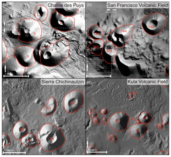
Figure 3.
Examples of the DTMs of the four areas; examined cones are outlined in red. The borders of DTMs with different resolutions available in each area are marked with a white-hatched line (a) Chaîne des Puys, (b) San Francisco Volcanic Field, (c) Sierra Chichinautzin and (d) Kula Volcanic Field).
3.2. Classical Approach in Scoria Cone Morphometry
3.2.1. Parameter Calculations
Settle described the classical morphometric parameters as follows. Cone height (Hco) is the difference between the maximum value of the crater rim, or the summit elevation and the average basal elevation. Cone width/basal diameter (Wco) is defined as the mean of the maximum and the minimum diameters. Crater width/diameter (Wcr) is the mean of the maximum and minimum diameters. Crater depth (Dcr) is the difference between the maximum rim or summit elevation and the lowest elevation in the crater [14]. Slope angles (which can be described as one of the most useful parameters [13]) were measured in the field or were calculated from the topographic maps’ contour lines [1,2]. Hasenaka and Carmichael [56] determined the calculations of the average slope values (Save) using the following formulas:
and
Save = tan−1[2Hco/(Wco − Wcr)],
Save = tan−1[2Hco/Wco]
Equation (1) should be used in the cases of cratered volcanoes.
3.2.2. Mann–Whitney Statistical Test
The Mann–Whitney test is the non-parametric equivalent of the two-sample t-test and applies to populations with unknown distributions and ordinal variables. It is used to test the null hypothesis that the two samples come from the same population. In this case, the significance level is set at 0.05.
Hooper and Sheridan performed this statistical analysis on both (San Francisco and Springerville) volcanic areas they studied for Hco/Wco ratios, maximum and average slope angle values. Since, except for the Early Pleistocene–Late Pliocene and Pliocene age group pairs (for maximum slope angle values), the test showed differences in the distributions for each pair, these authors found that the differences of age groups can be considered statistically significant [16].
3.3. New Symmetry Approaches in Scoria Cone Morphometry
Even if some studies considered the base level of scoria cones to not be horizontal [17], most of the previous research treated scoria cones as regular cones ignoring the possible asymmetry for various reasons. We suggest that it is equally important to make these symmetry tests, and to test the shape of the scoria cones together with the classical methods.
3.3.1. Detecting the Base Contour and the Centre Coordinates
Even in classical morphometric tests, the “step zero” is to determine the outline of the cones. This is one of the most critical steps in the processing, as many calculated or derived parameters depend on it.
For terrestrial volcanoes (thus scoria cones), an evident change in slope angle usually indicates the bottom of the volcanic cone. In most cases, this sudden angle change can be determined with the help of a shaded relief DTM map and a slope angle map. Therefore, with visual evaluation (of course depending on the resolution of the terrain model) it is possible to detect the base contours of the cones, even if the original base of the cone is not horizontal. It is somewhat easier to outline the crater rim (if any).
For a visual evaluation, it is common to set a centroid for each cone. For more elaborated studies usually (symmetry) centre coordinates are defined. The relative direction of an axis of symmetry (crossing the centre point) can also be determined manually or automatically, for example based on a specific observation, within a specified angular accuracy [57]. Another approach is presented in this article.
3.3.2. Polar Coordinate-Transformed Maps
The polar coordinate system transformation was introduced into volcanic morphometry by Székely and Karátson [58] and was used later [59]. This method, which has long been known and used in mathematics, can be used to investigate the symmetry of roughly circular symmetric shapes.
Given a roughly circular shape (in this case, a cone), the centre and the shape’s outline need to be defined using some tools providing a georeferenced output (see above). These features are all in the Cartesian (metric) coordinate system. For the points resulting from the transformation, the same coordinates can be described by the distance (r (m)) from the given (predefined) centre (x0, y0) and an azimuth angle (horizontal angular deviation from 0°) φ[°].
The conversion can be given by the following two equations:
and
where r (radial distance) and φ (azimuth) are the new coordinates in the (new) polar coordinate system, X and Y are the original Cartesian coordinates of the point to be transformed. Equation (4) results φ in radians; if it is needed to be in degrees, the values have to be converted (5):
r = ((X − x0)2 + (Y − y0)2)0.5
φ = arctan((X − x0)/(Y − y0))
φdeg = φ × 180°/π
3.3.3. Spatial Elliptical Fourier Descriptors
Although the shapes of the scoria cones are generally considered regular, various types of asymmetries can be observed. Among others, the baseline or crater rim of a scoria cone (which can be defined as derived planar curves) is often more similar to an ellipse, not a regular circle. From a morphometric point of view, these contours can be approximated mathematically with regular shapes. This can be done in several ways; in this study, we applied the Spatial Elliptical Fourier Descriptors [60] that generalize the modelling of a polygon. This method was introduced in volcanic geomorphometry by Zarazúa-Carbajal and De la Cruz-Reyna [61]. The application of Spatial Elliptical Fourier Descriptors allows the experimenter to choose the level of detail (LOD) of the modelling: a mutilated Fourier approximation can be used to approximate the vertices of the shape (x(t), y(t)) so that
where
and
and the recapitulation for n goes up to a chosen N (hereafter referred to as harmonic, 0 < n ≤ N) that will define the LOD. A0, C0 and An, Bn, Cn, Dn values will be determined. If N = 1 the shape obtained will be an ellipse, and A0 and C0 will be the calculated centre. Based on the Nyquist–Shannon (sampling) theorem, a theoretical limit for N is determined by the sampling density of the shape vertices. In this study, the Python implementation of Spatial Elliptical Fourier Descriptors was applied [62].
(x(t), y(t)) = (A0 + Σ Xi, C0 + Σ Yi)
Xi = An cos ωnt + Bn sin ωnt
Yi = Cn cos ωnt + Dn sin ωnt,
In Table 1 a summary of the data of the studied volcanic areas can be seen.

Table 1.
Summary of the data of the studied volcanic areas.
4. Results
4.1. Results Based on the Classic Parameters
Altogether, 501 scoria cones were examined in the four volcanic areas: 283 from the San Francisco Field, 126 from Chichinautzin, 64 from Kula, and 28 from Chaîne des Puys. Similar to the classic studies, basal diameter and cone height (Figure 4a) and from these, Hco/Wco ratio (Figure 4b) were calculated. Mann–Whitney tests were performed to detect significant differences between the groups of Hco/Wco ratios. Only one of the six pairs had p > 0.05—in the case of pair Chichinautzin and Chaîne des Puys p = 0.07346 (Figure 4b). For simplicity, in this comparison, the age groups were ignored.
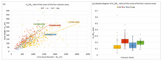
Figure 4.
(a) Hco/Wco ratio, (b) boxplot diagram of Hco/Wco ratios of the four volcanic areas (yellow: San Francisco, red: Chichinautzin, blue: Kula, green: CdP).
In previous research, the differences between the calculation methods of Hasenaka and Carmichael [56] and DTM-derived average slope values were shown [63,64]. In most cases, classical calculations gave values that differed (even significantly) from reality, so in this work, slope angle values calculated from the DTMs were used.
In Figure 5, the average slope values can be seen in boxplot diagrams, grouped by volcanic areas and age groups. In all cases, as the ages increase from left to right, a general trend (inverse relationship) of cone age–average slope exists.
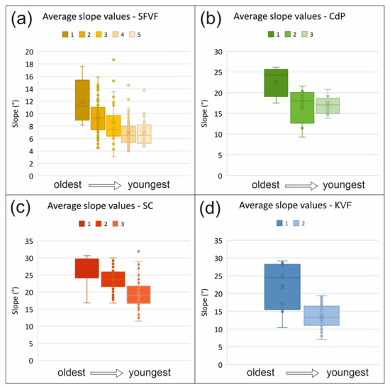
Figure 5.
Boxplot diagrams of average slope values grouped by age groups (in increasing order) and areas (a) Chaîne des Puys, (b) San Francisco Volcanic Field, (c) Sierra Chichinautzin and (d) Kula Volcanic Field).
We also performed the Mann–Whitney test for the groups shown in Figure 5. The p values calculated for each group can be seen in Table 2.
Table 2.
Calculated p values of average slope for each group pairs (grouped by areas). Significant differences are in red.
Table 2 shows that the distributions of slope angles are significantly different for all but three pairs of groups in each volcanic field pair. These three groups (San Francisco and Chaîne des Puys) are the oldest pairs in both cases.
4.2. Results of the New Approaches
4.2.1. Polar Coordinate-Transformed Maps
In Figure 6, we can see four selected scoria cones (one from each area) represented by polar coordinate transformation on the left side, while displayed in 3D on the right side. Certain features are highlighted with red ellipses/arrows, while the edge of the cone (base contour) is indicated with a dashed line. If the coordinates of the centre have been chosen correctly, in the case of relatively circularly symmetric cones the crater rim (here in white) will appear as a linear feature parallel to the x (directional) axis.
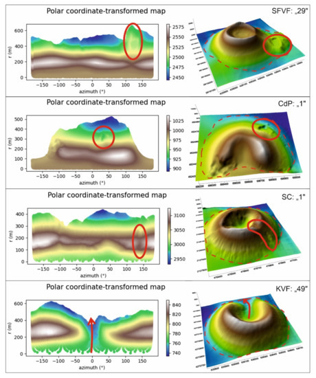
Figure 6.
Polar coordinate-transformed maps of four selected cones from each area. The outline of the cones can be seen with a red dashed line; local features are highlighted with a circle/arrow.
4.2.2. Spatial Elliptical Fourier Descriptors
Spatial Elliptical Fourier Descriptors calculated two harmonics: the first harmonic, which gives the fitted ellipse, from which ellipticity minor and major axes can be calculated, and the last (maximum) harmonic, which is determined by the Nyquist frequency. In Figure 7, the above-represented four selected cones can be seen with not only the first harmonic (blue line) and the last (n) harmonic (yellow line), but with the original contour line (red line above the yellow) and the second harmonic (green).
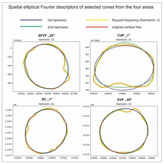
Figure 7.
Spatial Elliptical Fourier Descriptors of four selected cones from each area. Blue represents first, green second harmonic, red is the original contour line, and yellow is the harmonic that corresponds to the Nyquist frequency of the shape (N). Note that there is no practical difference between the actual contour line and the last (maximum) harmonic; in other words, this latter curve is a very good approximation of the contour.
In connection with this, the centre coordinates of the ellipse fitted to the given outline (in this case, the base contour and the crater contour) were also calculated. To increase the level of detail, the last harmonic was also calculated. In Figure 8, the distances of the two differently calculated base centre coordinates can be seen. It shows the distances of the original (visual evaluation) and the base contour’s fitted ellipse’s centre coordinates. In the cases of San Francisco and Chaîne des Puys, differences of several hundred meters can occur, while in the case of the other two, this difference remains mostly below one hundred metres.
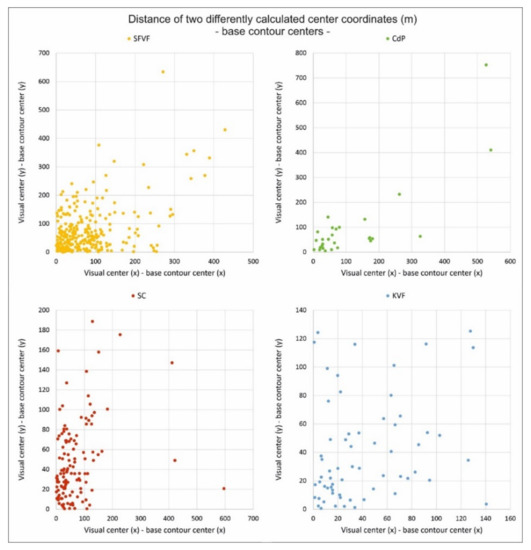
Figure 8.
Distance of two differently calculated base contour centre coordinates.
In Figure 9, the results of the same calculation applied on the crater rims are visualized; the distances of the original (visual interpretation) and Spatial Elliptical Fourier Descriptor-calculated centres of the crater rims are plotted. The difference between the craters is already within a smaller interval: here, too, San Francisco has the largest one, but it is below 400 m.
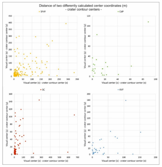
Figure 9.
Distance of two differently calculated crater centre coordinates.
We plotted the ellipticity of the two contours on a boxplot diagram (Figure 10a,b). Ellipticity can be calculated from the minor and major axes. For both the base and the crater, we cannot see significant differences in the distributions. However, it is remarkable that there are numerous outliers in all the volcanic fields indicating rather elliptic shapes. This observation also emphasizes that similar analyses of asymmetry would be necessary in the future. In Figure 10c, the directions (from north = 0°) of the ellipses fitted to the outlines can be seen. In the cases of Chaîne des Puys and Kula, some kind of difference can be seen. In the case of the former, a higher frequency of eastward elongation seems to be typical, while in Kula this occurs rather in the NE direction (we think this is partly a predominant wind-related feature [65], with possibly a tectonic imprint [66]). For Chichinautzin, the elongations are typically towards a NNW-SSE direction. Nevertheless, there was no statistical test performed to check whether this indication was statistically significant.
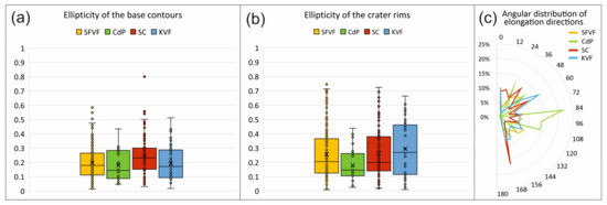
Figure 10.
Ellipticity of (a) base contours and (b) crater rims; (c) orientation of symmetry axes of the base contour.
5. Discussion
In the classic studies [1,2,6,7,13,14], Hco/Wco ratios were considered one of the most important descriptors of the geometry of the cones. Following Porter [6], who determined the average as 0.18 for 30 cones, these studies reported various, but similar average values. In an earlier study [18], a dependence on DTM resolution was also detected. In this study, we can also state that the four volcanic fields behave differently if we consider the regression line for all the cones (Figure 4a); the average values of Hco/Wco range from 0.10 to 0.23.
A better, more robust approach is to analyse the slope angles directly. Having the basic assumption that a relationship exists between ages and slope angles, it is straightforward to study the age groups separately [16]. As we have seen in Section 3.1., in harmony with similar results published earlier [16], the age groups show statistically significant differences in terms of slope angles. It is an expected result that slope angles decrease with cone age (e.g., [67]), but in this study, we focused instead on their distributions, and whether any behaviour pattern between age groups could be identified. This seems to be a useful approach; while there may be some overlap in distributions, typically even the slope angle distributions of the adjacent time groups are significantly different.
This general observation prompted us to combine the groups of the studied volcanic fields under study and examine how this produced an overall picture.
For Figure 11, the slope distributions of the age groups of the four examined areas have been arranged from the youngest (left) to the oldest (right) arranged by age in increasing order. The decreasing trend shown in Figure 5 can be observed here as well, but with an exception; the Chichinautzin groups do not fit into this pattern. In themselves, they show a similar trend, but their heteroscedastic character (large and varying scatter) is obvious.
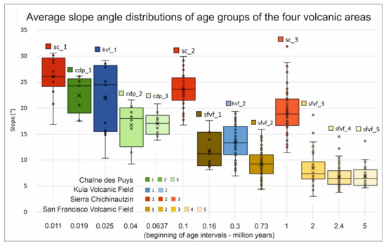
Figure 11.
Boxplot diagram of the average slope values of all the four areas and all age groups: Chichinautzin (SC) is marked with reddish shades, Chaîne des Puys (CdP) with greenish, Kula (KVF) with bluish, and San Francisco (SFVF) with brownish-yellowish. Age groups are arranged in increasing order (starting with the oldest).
Table 3 was prepared similarly to the previous one, now with the comparison of the p values of all groups. In this case, not only the local significant differences can be shown, but also the comparison of the areas.
Table 3.
Calculated p values of average slope for each group pair. Significant differences are in red.
Table 3 demonstrates that the ordering has more intrinsic value. The relative ordering of two selected slope distributions is verified by the Mann–Whitney test of selected pairs in many cases based on solely the distribution of average slopes. This result is remarkable because the studied volcanic fields have quite different characteristics in many senses (geological, lithological, climatic, etc.). In this study, we intentionally neglected these other characteristics, in order to focus on the slope distributions.
Although the distributions in Figure 11 show roughly the same trend in age and slope distribution for all four areas, the time intervals for Sierra Chichinautzin are strikingly different from the other three areas. This peculiar trend of SC can only be detected in the comparison with the other distributions. Since the studied volcanic fields differ in many respects, we would expect them to follow a general trend (Figure 5), but each would have its own specific distribution. In contrast, it is indeed the unexpected result of the present study that the integrated behaviour of the three areas shows similarities. On the other hand, the peculiar behaviour of SC suggests that since there are only four areas in the present study, there may be volcanic fields that tend to reinforce this SC trend. This also implies that it would be advisable to include more volcanic fields in future studies.
Since the ordering of the distributions by increasing age intervals is not robust enough (after all, it essentially depends only on the age of the oldest cone), a slightly more robust approach was tried. We also put the slope distributions in ascending order of age by the midpoint of the time intervals (see intervals in Figure 2), as shown in Figure 12. Note that there is only one swap compared to the previous ordering: CdP_1 swaps with KVF_1; i.e., the trend essentially remains similar.
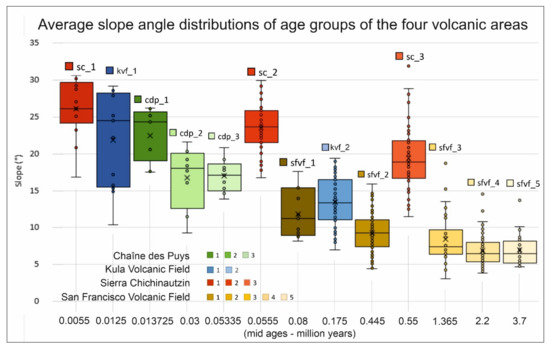
Figure 12.
Boxplot diagram of the average slope values of all the four areas and all age groups: Chichinautzin (SC) is marked with reddish shades, Chaîne des Puys (CdP) with greenish, Kula (KVF) with bluish, and San Francisco (SFVF) with brownish-yellowish. Age groups are arranged in ascending order (starting with the oldest age) by the midpoint of the time intervals (see intervals in Figure 2).
A possible explanation for this behaviour could be that in the four volcanic fields the asymmetries of the cones have an influence on the slopes and this relationship could affect the distribution. This effect is, however, unlikely to be present because the tests for asymmetries (Figure 8, Figure 9 and Figure 10) do not show too big differences, especially in terms of ellipticity (Figure 10a,b).
Another observation can be made based on Figure 11. As age increases, the slope distributions become progressively narrower, in line with the trend. In general the individual cones of the various volcanic fields testify that slope angles decrease with age [16,67]. What we tried here was to compare together all the age groups of these completely different volcanic fields. If this trend can be verified, the increasing age (in terms of distributions) may imply that the slope angles tend to become more and more similar, regardless of the variations of the initial shapes of the scoria cones (constrained by eruptive activity). A possible way to quantify this is to look at the interquartile range (IQR) of the distributions (Figure 13).
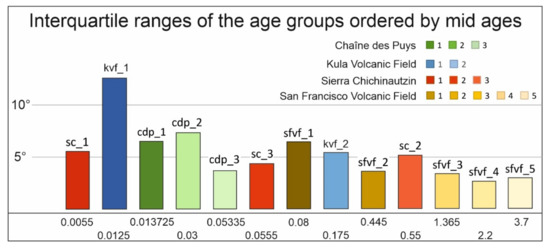
Figure 13.
The interquartile ranges of the distributions of the age groups: reddish shades are Chichinautzin, greenish are Chaîne des Puys, bluish are Kula, and (brownish) yellowish are San Francisco age groups.
The interquartile ranges were sorted by the age order mentioned above, by the midpoint of the time intervals. First, we omitted Chichinautzin age groups because of their particular, heteroscedastic behaviour apparent in Figure 12, and in this way, we obtained the set of interquartile ranges of 10 age groups. This set of samples is a low number in a statistical sense, so one can apply only tests that are robust enough, e.g., the above-used Mann–Whitney test, which is suitable for this purpose. (Here we used vassarstats.net webpage [68].)
The ordered set of 10 interquartile ranges was split in the middle to form Group A and Group B (5 values each) and the test was performed on these two groups with the initial hypothesis H0 that these two groups were coming from different distributions. As the Mann–Whitney test is nonparametric, we do not have to know anything about the original distribution(s). Based on the test result of UA = 1 (with critical interval for UA from 4 to 21) and the resulting p = 0.0107, one can conclude that Group A and Group B come from different distributions. In other words, the older group has significantly different (lower) slope distribution interquartile ranges than the younger groups.
This motivating result led us to re-include the Chichinautzin age groups (Figure 13) and retest the larger sample. Then, altogether we investigated 13 interquartile ranges that has been split into 7 and 6, also ordered by the mid-ages of the groups. Although we observed the heteroscedastic behaviour of the Chichinautzin groups, the interquartile ranges of this volcanic field seemed to fit to the trend. In addition, the split was verified by the Mann–Whitney test, proving the high probability of the difference (and therefore its significance).
The results of these two Mann–Whitney tests (Table 4) suggest that the ordering is probably correct and, consequently, the trend of the interquartile ranges that seem to be related to the mid-age of the groups might be a valid trend. Unfortunately, we cannot make a stronger statement than this due to the small sample size. By including further scoria cones of other volcanic fields, new studies could prove or disprove our hypothesis.
Table 4.
Calculated p and u values (and the sample sizes) of interquartile ranges (Groups A and B). Significant differences are in red.
In the previous observation that slope angle distributions will be narrower with age, regardless of which one of the four volcanic fields is considered, it is worth considering the idea that the horizontal shape of the cones may converge to a more symmetric one with increasing age. Based on the results of our study, however, this conclusion cannot be drawn yet. As we have seen in the various asymmetry calculations, there are numerous outliers and, most probably, the distributions of the ellipticities and centroid positions are special, non-Gaussian distributions, and they are most probably skewed. Further experiments are needed to detect how the original elongations (due to Hawaiian fountain fire activity/fissure formation [67]) are modified with time.
6. Conclusions
Based on the observations and calculations of this study, we can conclude as follows:
- Whereas the individual behaviour of the slope patterns of scoria cones may vary and old and young cones may show similar morphometric values, the distributions of the average slope angles of the cone age groups follow a trend. According to the statistical tests, the distribution of the slope angles of the older groups is significantly different from the younger ones, with slope angles tending to decrease towards the older groups.
- Applying our innovative idea, to merge the age groups of all four volcanic areas into a combined dataset and treating the age groups independently from the specific area, the distributions ordered by the increasing mid-period age show a similar trend with decreasing median values, except for Sierra Chichinautzin. The latter area shows heteroscedastic but also trend-like behaviour.
- From the study of the interquartile ranges (IQR) of the average slope distributions, we can conclude that not only the median values of the slope distributions decrease with increasing mid-period age, but they also become more uniform with age, with the interquartile range of slopes decreasing in a trend-like manner.
We speculate that there may be volcanic fields that tend to reinforce this type of trend rather than that of the other three volcanic fields. This also suggests that it is reasonable to consider further volcanic fields in the future in order to determine whether more than one such trend exists and, if so, what is common and what is different in the behaviour of these distributions. Our results show that a robust relationship between the distributions of the shape properties of scoria cones and their age groups can be successfully established with this method.
Author Contributions
Conceptualization, B.S.; methodology, F.V. and B.S.; software, F.V. and B.S.; validation, all; formal analysis, F.V. and B.S.; investigation, F.V. and B.S.; resources, all; data curation, F.V. and B.S.; writing—original draft preparation, F.V.; writing—review and editing, all; visualization, F.V.; funding acquisition, B.S. All authors have read and agreed to the published version of the manuscript.
Funding
This research received no external funding.
Data Availability Statement
Data will be made available on request.
Acknowledgments
F.V. was supported by project no. TKP2021-NVA-29, which has been implemented with the support provided by the Ministry of Innovation and Technology of Hungary from the National Research, Development, and Innovation Fund, financed under the TKP2021-NVA funding scheme. This work is partly carried out as a contribution to the UNESCO International Geosciences Programme project 692 ‘Geoheritage for Resilience’ (www.geopoderes.com, accessed on 28 November 2022). Gustavo Vivó Vázquez is thanked for his initial work on the Lidar dataset of the Sierra Chichinautzin. M.N.-G. received funding from the project: UNAM DGAPA PAPIIT IN103421.
Conflicts of Interest
The authors declare no conflict of interest. The funders had no role in the design of the study; in the collection, analyses, or interpretation of data; in the writing of the manuscript; or in the decision to publish the results.
References
- Wood, C.A. Morphometric evolution of cinder cones. J. Volcanol. Geotherm. Res. 1980, 7, 387–413. [Google Scholar] [CrossRef]
- Wood, C.A. Morphometric analysis of cinder cone degradation. J. Volcanol. Geotherm. Res. 1980, 8, 137–160. [Google Scholar] [CrossRef]
- Székely, B.; Király, E.; Karátson, D.; Bata, T. A parameterisation attempt of scoria cones of the San Francisco Volcanic Field (Arizona, USA) by conical fitting. In Proceedings of the Proceedings of Geomorphometry, Zurich, Switzerland, 31 August–2 September 2009; Purves, R., Gruber, S., Hengl, T., Straumann, R., Eds.; Department of Geography, University of Zurich: Zurich, Switzerland, 2009; pp. 178–182. [Google Scholar]
- Vörös, F.; Koma, Z.; Székely, B. The application of polar coordinate transformation on the cinder cones of the San Francisco Volcanic Field. In Proceedings of the Student V4 Geoscience Conference and Scientific Meeting GISÁČEK: Conference Proceedings, Ostrava, Czech Republic, 22 March 2017; Tesla, J., Ed.; Institute of Geoinformatics, Technical University of Ostrava: Ostrava, Czech Republic, 2017; pp. 102–110. [Google Scholar]
- Székely, B.; Vörös, F. Studying the distributions of DTM derivatives of cinder cones: A statistical approach in volcanic morphometry. EGU Gen. Assem. 2020, 2020, 10465. [Google Scholar] [CrossRef]
- Porter, S.C. Distribution, morphology, and size frequency of cinder cones on Mauna Kea volcano, Hawaii. Bull. Geol. Soc. Am. 1972, 83, 3607–3612. [Google Scholar] [CrossRef]
- Colton, S.H. The basaltic cinder cones and lava flows of the San Francisco Mountain volcanic field. Museum North. Arizona Bull. 1967, 10, 1–49. [Google Scholar]
- Kear, D. Erosional stages of volcanic cones as indicators of age. N. Z. J. Sci. Tech. 1957, 38, 671–682. [Google Scholar]
- Segerstrom, K. Erosion Studies at Paricutin, State of Michoacán, Mexico. U. S. Geol. Surv. Bull. 1950, 965, 1–163. [Google Scholar] [CrossRef]
- Segerstrom, K. Erosion and related phenomena at Parıcutin in 1957. U. S. Geol. Surv. Bull. 1960, 1104, 1–18. [Google Scholar]
- Segerstrom, K. Parıcutin, 1965-Aftermath of eruption. U. S. Geol. Surv. Prof. Pap. 1966, 550, 93–101. [Google Scholar]
- Bloomfield, K. A late-Quaternary monogenetic volcano field in central Mexico. Geol. Rundsch. 1975, 64, 476–497. [Google Scholar] [CrossRef]
- Scott, D.H.; Trask, N.J. Geology of the Lunar Crater Volcanic Field, Nye County, Nevada. U. S. Geol. Surv. Prof. Pap. 1971, 599, 22. [Google Scholar]
- Settle, M. The structure and emplacement of cinder cone fields. Am. J. Sci. 1979, 279, 1089–1107. [Google Scholar] [CrossRef]
- Moore, R.B.; Wolfe, E. Geologic Map of the Eastern San Francisco Volcanic Field, Arizona, Scale 1:50 000; U. S. Geological Survey: Reston, VA, USA, 1976. [Google Scholar]
- Hooper, D.M.; Sheridan, M.F. Computer-simulation models of scoria cone degradation. J. Volcanol. Geotherm. Res. 1998, 83, 241–267. [Google Scholar] [CrossRef]
- Favalli, M.; Karátson, D.; Mazzarini, F.; Pareschi, M.T.; Boschi, E. Morphometry of scoria cones located on a volcano flank: A case study from Mt. Etna (Italy), based on high-resolution LiDAR data. J. Volcanol. Geotherm. Res. 2009, 186, 320–330. [Google Scholar] [CrossRef]
- Fornaciai, A.; Favalli, M.; Karátson, D.; Tarquini, S.; Boschi, E. Morphometry of scoria cones, and their relation to geodynamic setting: A DEM-based analysis. J. Volcanol. Geotherm. Res. 2012, 217–218, 56–72. [Google Scholar] [CrossRef]
- Vörös, F.; van Wyk de Vries, B.; Székely, B. Geomorphometric descriptive parameters of scoria cones from different DTMs: A resolution invariance study. In Proceedings of the 7th International Conference on Cartography and GIS, Sozopol, Bulgaria, 18–23 June 2018; Bandrova, T., Konečný, M., Eds.; pp. 603–612. [Google Scholar]
- Priest, S.; Duffield, W.; Malis-Clark, K.; Hendley, J., II; Stauffer, P. The San Francisco Volcanic Field, Arizona; U. S. Geological Survey Fact Sheet 017-01; USGS: Reston, VA, USA, 2001. [Google Scholar] [CrossRef]
- Bata, T. Morfometriai Paraméterek Meghatározása Vulkáni Kúpokon a San Francisco Vulkáni Terület (USA, Arizona) Példáján. Master’s Thesis, Eötvös Loránd Tudományegyetem, Budapest, Hungary, 2007. [Google Scholar]
- Wood, C.A.; Baldridge, S. Volcano tectonics of the Western United States. In Volcanoes of North America; Wood, C.A., Kienle, J., Eds.; Cambridge Univ Press: Cambridge, UK, 1990; pp. 147–154. [Google Scholar]
- Karátson, D.; Telbisz, T.; Singer, B.S. Late-stage volcano geomorphic evolution of the Pleistocene San Francisco Mountain, Arizona (USA), based on high-resolution DEM analysis and 40Ar/39Ar chronology. Bull. Volcanol. 2010, 72, 833–846. [Google Scholar] [CrossRef]
- Wolfe, E.W.; Ulrich, G.E.; Holm, R.F.; Moore, R.B.; Newhall, C.G. Geologic map of the central part of the San Francisco Volcanic Field, north-central Arizona. Misc. F. Stud. Map 1987. [Google Scholar] [CrossRef]
- Tanaka, K.L.; Shoemaker, E.M.; Ulrich, G.E.; Wolfe, E.W. Migration of Volcanism in the San-Francisco Volcanic Field, Arizona. Geol. Soc. Am. Bull. 1986, 97, 129–141. [Google Scholar] [CrossRef]
- Del Pozzo, A.L.M. Monogenetic vulcanism in sierra Chichinautzin, Mexico. Bull. Volcanol. 1982, 45, 9–24. [Google Scholar] [CrossRef]
- Siebe, C.; Rodríguez-Lara, V.; Schaaf, P.; Abrams, M. Radiocarbon ages of Holocene Pelado, Guespalapa and Chichinautzin scoria cones, south of Mexico city: Implications for archaeology and future hazards. Bull. Volcanol. 2004, 66, 203–225. [Google Scholar] [CrossRef]
- Agustín-Flores, J.; Siebe, C.; Guilbaud, M.N. Geology and geochemistry of Pelagatos, Cerro del Agua, and Dos Cerros monogenetic volcanoes in the Sierra Chichinautzin Volcanic Field, south of México City. J. Volcanol. Geotherm. Res. 2011, 201, 143–162. [Google Scholar] [CrossRef]
- Lorenzo-Merino, A.; Guilbaud, M.N.; Roberge, J. The violent Strombolian eruption of 10 ka Pelado shield volcano, Sierra Chichinautzin, Central Mexico. Bull. Volcanol. 2018, 80, 27. [Google Scholar] [CrossRef]
- Guilbaud, M.N.; Arana-Salinas, L.; Siebe, C.; Barba-Pingarrón, L.A.; Ortiz, A. Volcanic stratigraphy of a high-altitude Mammuthus columbi (Tlacotenco, Sierra Chichinautzin), Central México. Bull. Volcanol. 2015, 77, 17. [Google Scholar] [CrossRef]
- Siebe, C.; Arana-Salinas, L.; Abrams, M. Geology and radiocarbon ages of Tláloc, Tlacotenco, Cuauhtzin, Hijo del Cuauhtzin, Teuhtli, and Ocusacayo monogenetic volcanoes in the central part of the Sierra Chichinautzin, México. J. Volcanol. Geotherm. Res. 2005, 141, 225–243. [Google Scholar] [CrossRef]
- Wallace, P.J.; Carmichael, I.S.E. Quaternary volcanism near the Valley of Mexico: Implications for subduction zone magmatism and the effects of crustal thickness variations on primitive magma compositions. Contrib. Mineral. Petrol. 1999, 135, 291–314. [Google Scholar] [CrossRef]
- Schaaf, P.; Stimac, J.; Siebe, C.; Macías, J.L. Geochemical evidence for mantle origin and crustal processes in volcanic rocks from Popocatépetl and surrounding monogenetic volcanoes, central Mexico. J. Petrol. 2005, 46, 1243–1282. [Google Scholar] [CrossRef]
- Siebe, C. Age and archaeological implications of Xitle volcano, southwestern Basin of Mexico-City. J. Volcanol. Geotherm. Res. 2000, 104, 45–64. [Google Scholar] [CrossRef]
- Arce, J.L.; Layer, P.W.; Lassiter, J.C.; Benowitz, J.A.; Macías, J.L.; Ramírez-Espinosa, J. 40Ar/39Ar dating, geochemistry, and isotopic analyses of the quaternary Chichinautzin volcanic field, south of Mexico City: Implications for timing, eruption rate, and distribution of volcanism. Bull. Volcanol. 2013, 75, 774. [Google Scholar] [CrossRef]
- Vivó Vázquez, G. Variabilidad Geomorfológica de los Conos de Escoria de la Porción Centro-Oriental de la Sierra Chichinautzin a Partir de Modelos Digitales de Elevación; Universidad Nacional Autónoma de México: Mexico City, Mexico, 2017. [Google Scholar]
- Arce, J.L.; Muñoz-Salinas, E.; Castillo, M.; Salinas, I. The ~2000 yr BP Jumento volcano, one of the youngest edifices of the Chichinautzin Volcanic Field, Central Mexico. J. Volcanol. Geotherm. Res. 2015, 308, 30–38. [Google Scholar] [CrossRef]
- Jolivet, L.; Faccenna, C.; Huet, B.; Labrousse, L.; Le Pourhiet, L.; Lacombe, O.; Lecomte, E.; Burov, E.; Denèle, Y.; Brun, J.P.; et al. Aegean tectonics: Strain localisation, slab tearing and trench retreat. Tectonophysics 2013, 597–598, 1–33. [Google Scholar] [CrossRef]
- Özpolat, E.; Yıldırım, C.; Görüm, T.; Gosse, J.C.; Şahiner, E.; Sarıkaya, M.A.; Owen, L.A. Three-dimensional control of alluvial fans by rock uplift in an extensional regime: Aydın Range, Aegean extensional province. Sci. Rep. 2022, 12, 15306. [Google Scholar] [CrossRef]
- Hamilton, W.J.; Strickland, H.E. On the Geology of Western Part of Asia Minor. Trans. Geol. Soc. London 1841, I, 81. [Google Scholar] [CrossRef]
- Washington, H.S. The Volcanoes of the Kula Basin in Lydia; University of Leipzig: Leipzig, Germany, 1893. [Google Scholar]
- Erinç, S. Kula ve Adala arasinda gene, volkan reliyefi. Istanbul Üniversitesi Cograf. Enstitüsü Derg. 1970, 9, 7–32. [Google Scholar]
- Bunbury, J.M.; Hall, L.; Anderson, G.J.; Stannard, A. The determination of fault movement history from the interaction of local drainage with volcanic episodes. Geol. Mag. 2001, 138, 185–192. [Google Scholar] [CrossRef]
- Westaway, R.; Guillou, H.; Yurtmen, S.; Beck, A.; Bridgland, D.; Demir, T.; Scaillet, S.; Rowbotham, G. Late Cenozoic uplift of western Turkey: Improved dating of the Kula Quaternary volcanic field and numerical modelling of the Gediz River terrace staircase. Glob. Planet. Chang. 2006, 51, 131–171. [Google Scholar] [CrossRef]
- Westaway, R.; Pringle, M.; Yurtmen, S.; Demir, T.; Bridgland, D.; Rowbotham, G.; Maddy, D. Pliocene and Quaternary regional uplift in western Turkey: The Gediz River terrace staircase and the volcanism at Kula. Tectonophysics 2004, 391, 121–169. [Google Scholar] [CrossRef]
- Ulusoy, İ.; Sarıkaya, M.A.; Schmitt, A.K.; Şen, E.; Danišík, M.; Gümüş, E. Volcanic eruption eye-witnessed and recorded by prehistoric humans. Quat. Sci. Rev. 2019, 212, 187–198. [Google Scholar] [CrossRef]
- Richardson-Bunbury, J.M. The Kula Volcanic Field, western Turkey: The development of a Holocene alkali basalt province and the adjacent normal-faulting graben. Geol. Mag. 1996, 133, 275–283. [Google Scholar] [CrossRef]
- Şen, E.; Erturaç, M.K.; Gümüş, E. Quaternary Monogenetic Volcanoes Scattered on a Horst: The Bountiful Landscape of Kula. World Geomorphol. Landscapes 2019, 577–588. [Google Scholar] [CrossRef]
- Şen, E.; Aydar, E.; Bayhan, H.; Gourgaud, A. Volcanological characteristics of alkaline basalt and pyroclastic deposits, Kula volcanoes, western Anatolia. Yerbilimleri 2014, 35, 219–252. [Google Scholar]
- Accueil|Craig. Available online: https://www.craig.fr/ (accessed on 29 April 2021).
- 2011_Site_Puy_De_Dome_Lidarverne-Fichiers-Drive Opendata du CRAIG. Available online: https://drive.opendata.craig.fr/s/opendata?path=%2Flidar%2Fautres_zones%2F2011_site_puy_de_dome_lidarverne (accessed on 27 April 2021).
- TNM Download v2. Available online: https://apps.nationalmap.gov/downloader/#/ (accessed on 20 August 2022).
- 1 Meter Digital Elevation Models (DEMs)-USGS National Map 3DEP Downloadable Data Collection|USGS Science Data Catalog. Available online: https://data.usgs.gov/datacatalog/data/USGS:77ae0551-c61e-4979-aedd-d797abdcde0e (accessed on 20 August 2022).
- 1/3rd Arc-Second Digital Elevation Models (DEMs)-USGS National Map 3DEP Downloadable Data Collection|USGS Science Data Catalog. Available online: https://data.usgs.gov/datacatalog/data/USGS:3a81321b-c153-416f-98b7-cc8e5f0e17c3 (accessed on 20 August 2022).
- Instituto Nacional de Estadística y Geografía (INEGI). Available online: https://www.inegi.org.mx/ (accessed on 29 September 2022).
- Hasenaka, T.; Carmichael, I.S.E. The cinder cones of Michoacán-Guanajuato, central Mexico: Their age, volume and distribution, and magma discharge rate. J. Volcanol. Geotherm. Res. 1985, 25, 105–124. [Google Scholar] [CrossRef]
- Karátson, D.; Németh, K.; Székely, B.; Ruszkiczay-Rüdiger, Z.; Pécskay, Z. Incision of a river curvature due to exhumed Miocene volcanic landforms: Danube Bend, Hungary. Int. J. Earth Sci. 2006, 95, 929–944. [Google Scholar] [CrossRef]
- Székely, B.; Karátson, D. DEM-based morphometry as a tool for reconstructing primary volcanic landforms: Examples from the Börzsöny Mountains, Hungary. Geomorphology 2004, 63, 25–37. [Google Scholar] [CrossRef]
- Székely, B.; Hampton, S.J. DEM-aided volcanic reconstruction and collapse recognition of degraded Miocene volcanic edifices: A case history of Lyttelton Volcano, New Zealand. Geophys. Res. Abstr. 2007, 9, 10295. [Google Scholar]
- Kuhl, F.P.; Giardina, C.R. Elliptic Fourier features of a closed contour. Comput. Graph. Image Process. 1982, 18, 236–258. [Google Scholar] [CrossRef]
- Zarazúa-Carbajal, M.C.; De la Cruz-Reyna, S. Morpho-chronology of monogenetic scoria cones from their level contour curves. Applications to the Chichinautzin monogenetic field, Central Mexico. J. Volcanol. Geotherm. Res. 2020, 407, 107093. [Google Scholar] [CrossRef]
- Grieve, S.W.D. Spatial-efd: A spatial-aware implementation of elliptical Fourier analysis. J. Open Source Softw. 2017, 2, 189. [Google Scholar] [CrossRef]
- Vörös, F.; de van Vries, B.W.; Karátson, D.; Székely, B. DTM-based morphometric analysis of scoria cones of the Chaîne des Puys (France)—the classic and a new approach. Remote Sens. 2021, 13, 1983. [Google Scholar] [CrossRef]
- Vörös, F.; Székely, B. High-resolution DTM-based estimation of geomorphometric parameters of selected putative martian scoria cones. Icarus 2022, 377, 114923. [Google Scholar] [CrossRef]
- Bemis, K.; Walker, J.; Borgia, A.; Turrin, B.; Neri, M.; Swisher, C. The growth and erosion of cinder cones in Guatemala and El Salvador: Models and statistics. J. Volcanol. Geotherm. Res. 2011, 201, 39–52. [Google Scholar] [CrossRef]
- Tibaldi, A. Morphology of pyroclastic cones and tectonics. J. Geophys. Res. Solid Earth 1995, 100, 24521–24535. [Google Scholar] [CrossRef]
- Becerra-Ramírez, R.; Dóniz-Páez, J.; González, E. Morphometric Analysis of Scoria Cones to Define the “Volcano-Type” of the Campo de Calatrava Volcanic Region (Central Spain). Land 2022, 11, 917. [Google Scholar] [CrossRef]
- Lowry, R. VassarStats: Website for Statistical Computation. Available online: http://vassarstats.net/ (accessed on 28 November 2022).
Publisher’s Note: MDPI stays neutral with regard to jurisdictional claims in published maps and institutional affiliations. |
© 2022 by the authors. Licensee MDPI, Basel, Switzerland. This article is an open access article distributed under the terms and conditions of the Creative Commons Attribution (CC BY) license (https://creativecommons.org/licenses/by/4.0/).