Article

Reconstruction of High-Resolution Sea Surface Salinity over 2003–2020 in the South China Sea Using the Machine Learning Algorithm LightGBM Model

1
State Key Laboratory of Marine Environmental Science and College of Ocean and Earth Sciences, Xiamen University, Xiamen 361102, China
2
Fujian Provincial Key Laboratory for Coastal Ecology and Environmental Studies, Xiamen University, Xiamen 361102, China
*
Author to whom correspondence should be addressed.
Remote Sens. 2022, 14(23), 6147; https://doi.org/10.3390/rs14236147
Submission received: 19 October 2022 / Revised: 16 November 2022 / Accepted: 1 December 2022 / Published: 4 December 2022

Abstract

:
Salinity, as one of the essential physical properties of seawater, is a common tracer differentiating water masses in the ocean, which often require relatively high-resolution datasets. Limited by the coverage of direct observations, however, high-resolution spatial and temporal salinity data are not always available, which hinders the fine application of salinity data in discerning ocean processes and improved modeling of ocean physics and biogeochemistry. To supplement the salinity database, we reconstructed sea surface salinity (SSS) with reasonably high spatial resolution (0.05° × 0.05°) over 2003–2020 in the South China Sea (SCS) with a machine learning algorithm based on a combination of MODIS-Aqua remote sensing data and a large cruise observation-based dataset. The reconstructed SSS has a mean absolute error (MAE) of 0.2 when compared with our underway observations with a corresponding root mean square error (RMSE) of 0.3. The MAE between station-based observations and our reconstruction was 0.5, and the RMSE was 0.7. These validations strongly suggest that our reconstruction is highly adequate, representing at most a quarter of the identified discrepancies compared to the remote sensing SSS or two other prevalent model-derived datasets. Based on our reconstruction, the SSS in the SCS is relatively low in coastal waters, but high in the ocean basin, with a seasonal pattern with a minimum in the summer and a maximum in the winter. This spatio-temporal distribution is well consistent with the observations and is affected by the Pearl River plume, sea surface circulation, and precipitation. Using our reconstructed SSS, we were able to successfully characterize the spreading of the Pearl River and Mekong River plumes and the intrusion of the Kuroshio Current from the Pacific Ocean into the SCS.

1. Introduction

Salinity, one of the basic physical properties of seawater, can be used to trace different water masses and infer chemical behaviors in the ocean, particularly in marginal seas [1,2]. Previous studies have found that the variability in salinity markedly influences regional circulation and climate [3,4]. Sea surface salinity (SSS) has been recognized as one of the essential climate variables by the Global Climate Observing System (GCOS) [5]. Traditional station-based or underway observations of SSS are usually ship time-consuming and thus costly and achieve only limited spatial and temporal coverage [6]. Satellite sensors have the advantages of real-time and high spatial coverage and have been applied more and more widely in the inversion of SSS over large spatial scales [7,8].
Two inversion methods, direct and indirect, are used in estimating SSS with remote sensing data [9,10]. The direct method mainly uses a salinity-sensitive band of satellites (e.g., near infrared and microwave L/S bands) to set up an inversion model between SSS and the spectral data using differential spectroscopy technology such as the sea surface radiation and multivariate statistical regression models [11,12,13,14,15]. In coastal areas, however, the SSS estimated using the direct method may be seriously biased by sea surface roughness and the land radio frequency [11,12,13,14,15]. As for the indirect method, in the early 21st century, a linear inversion model was initially set up based on the relationship between SSS and an ocean color remote sensing product, such as sea surface temperature (SST) or chlorophyll a [5,7,16]. However, in its early stages, this linear inversion method often considered only a single influencing factor and could not avoid the poor robustness induced by linear regressions [17,18,19]. With the development of machine learning, nonlinear regression models have been adopted. For example, Geiger et al. [17] developed a neural network model to estimate SSS in the Mid-Atlantic using normalized water-leaving radiance, SST, and MODIS-Aqua location information. Chen and Hu [20] constructed a multi-layer perceptual neural network (MPNN) inversion model to determine SSS based on remote sensing reflectance and SST from MODIS and SeaWiFS. Mu et al. [21] added SST as an independent machine learning variable in the SSS reconstruction, which effectively improved the SSS in the South China Sea (SCS) based on the SMOS (Soil Moisture and Ocean Salinity) satellite. These studies have shown that the absorption coefficient of colored detrital matter (aCDM), remote sensing reflectance, and SST are important parameters in the reconstruction of salinity, especially in coastal regions [22]. The SCS is the largest marginal sea of the North Pacific Ocean [4,23,24]. Due to complex atmospheric forces (e.g., seasonal monsoons with strong wind speeds), meso-scale processes (e.g., upwelling), and the spreading of river plumes, as well as the intrusion of the Kuroshio current, the circulation pattern in the SCS is quite complex [24,25,26,27]. To better understand the ocean dynamics and further reveal the influence of dynamic oceanic processes on biogeochemical cycles, it is necessary to obtain the SSS spatio-temporal structure [2,28]. At present, the remote sensing-derived salinity data in the SCS are based on the AQUARIUS/SAC-D mission, the Soil Moisture Active Passive (SMAP) mission and SMOS mission. The AQUARIUS/SAC-D mission consists of three passive microwave radiometers to detect the surface emission that was used to obtain salinity [29]. The SMAP mission includes an L-band radiometer and a high-resolution L-band radar [30]. The SMOS mission consists of the platform and payload, MIRAS (Microwave Imaging Radiometer using Aperture Synthesis), which is mounted on a standard spacecraft platform called Proteus [31]. These three missions all use the “skin” measurements, which means that all of them can only collect information about the sea surface [29,30,31]. To make these satellite-derived SSS data quantitatively consistent at appropriate temporal and spatial scales, the University of Hawaii at Manoa, in collaboration with Remote Sensing Systems, used an optimal interpolation method to produce a multi-satellite fusion salinity dataset (OISSS) with the three missions mentioned above [32,33]. However, this dataset was only available starting from 2011 [32,33]. Besides these remote sensing datasets, the Institute of Atmospheric Physics Ocean Salinity dataset (IAPOS) provides a model-based salinity dataset, which improved global ocean salinity estimates from 2000 to 2019, based on bias-corrected expendable bathythermograph (XBT) measurements from the World Ocean Database [34]. In addition, in the framework of the Copernicus Marine Environment Monitoring Service (CMEMS), an SSS dataset was produced using a multidimensional covariance model (MUL) within the MyOcean project [5,17]. Compared with the observational SSS data in the SCS, the three datasets, OISSS, IAPOS, and MUL, have root mean square errors (RMSE) of about 2 [17,32,33,34], which, together with their limited spatial resolution (the highest resolution is 0.25° × 0.25°), precludes differentiating some coastal plume waters and meso-scale processes. Furthermore, the accuracy of these three salinity datasets in the SCS remains to be verified.
To better serve oceanographic and subsequent climatic modeling purposes, in this study we reconstructed SSS in the SCS with a high spatial resolution, 0.05° × 0.05°, based on a machine learning algorithm, Light Gradient Boosting Machine (LightGBM), using 2003–2020 observational salinity data and satellite data. The spatial coverage of our reconstruction was 5–25°N, 109–122°E. We then compared the accuracy of our reconstructed dataset with that of the other three datasets (OISSS, IAPOS, and MUL). In the SCS, river plumes are mainly from the Pearl and the Mekong Rivers. The Mekong River Estuary is located at ~8°N, 106°E, i.e., outside our reconstruction domain. Thus, although the Mekong River is considered in showing the spatial distribution of our reconstructed SSS field, our main river plume focus in this study is the influence of the Pearl River plume.

2. Data

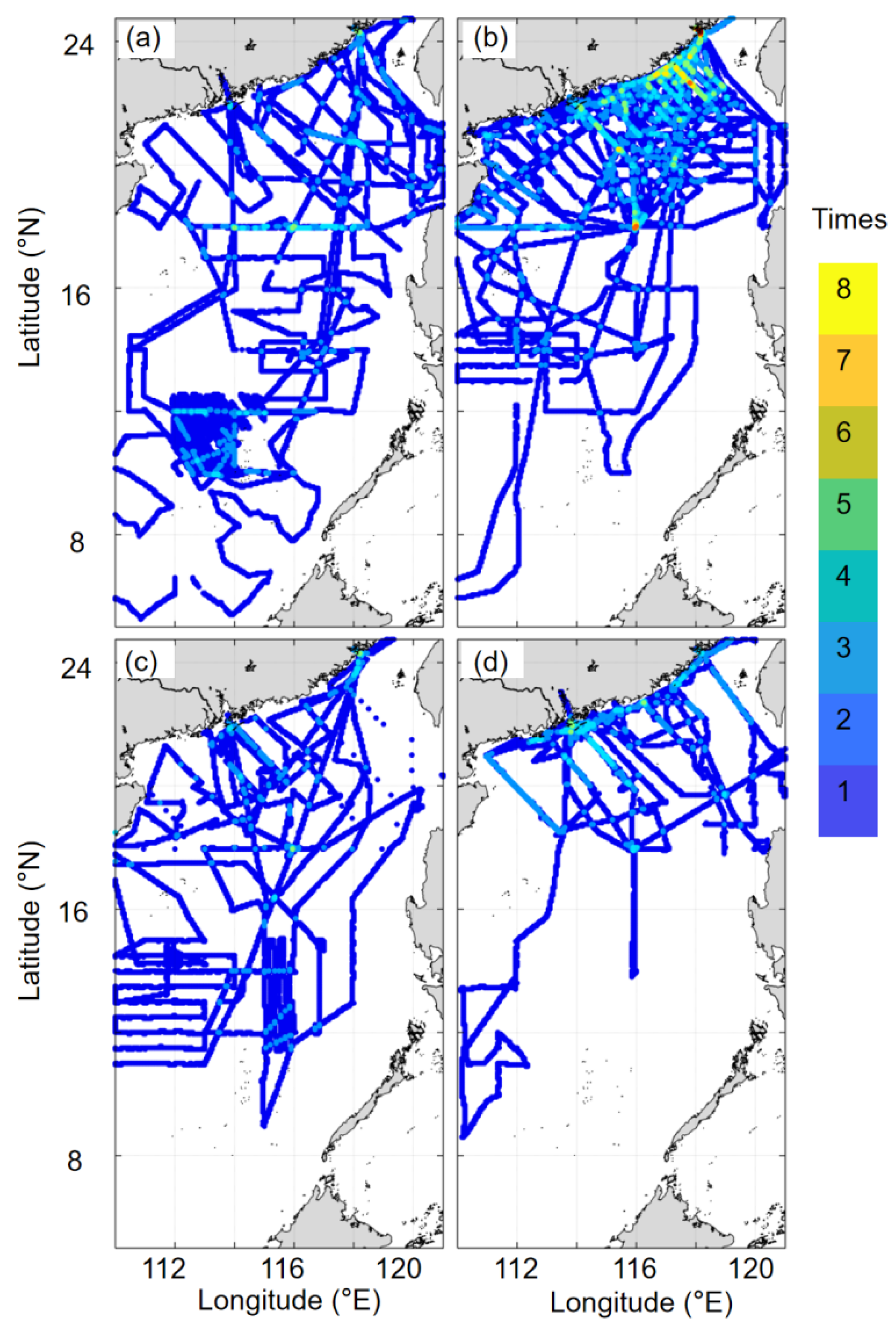
2.1. Observational Salinity Data

The underway SSS data collected from 40 cruises in the SCS from 2003 to 2020 onboard the R/Vs Dongfanghong 2, Yanping 2, Shiyan 3, Jiageng (TKK), Haijian 83, Haidiao 6, Haike 68, and Kexue 3 were compiled in this study (Table 1). Although the data before February 2018, except those collected in July 2005, June 2006, July 2015, and June 2017, are from Li et al. [6], this is the first time that their spatial distribution is shown. The data collected in July 2005, June 2006, July 2015, June 2017, and after February 2018 are reported here for the first time. The underway data were seasonally averaged, taking the mean from March through May as the spring data, June through August as the summer data, September through November as the fall data, and December through February (the following year) as the winter data. Spring data are available for the years 2004–2005, 2008–2009, 2011–2012, 2014, and 2020. Summer data correspond to 2004–2009, 2012, 2015–2017, and 2019–2020, fall data correspond to 2003–2004, 2006–2008, 2010, and 2020, while the winter data are for 2003, 2005–2006, 2008–2009, and 2017. The seasonal averaged SSS data were gridded into 0.05° × 0.05° grids. The spatial coverage and observation frequency of the underway SSS for each season differed over the years (Figure 1). The spring data had the largest space coverage, ~5–24.5°N, the summer data had the greatest survey frequency, while the winter data reflected the least frequent surveys and the least spatial coverage. The seasonal average survey coverage was less than 25% of our SCS domain, especially in the basin where the coverage was less than 10% in winter. Additionally, in the basin the survey frequency was only once or twice in each season, while it was up to eight times in coastal areas in the summer.
To verify the reliability of the reconstructed data, we divided the observational underway dataset into two subsets. One includes the data collected until February 2018, which were used in machine learning (named OB_A), and the other represents the data collected after February 2018, which were used as an independent dataset for validation (named OB_B). We also used station-based observational SSS data and SOCAT (Surface Ocean CO2 Atlas) underway SSS data as additional validation datasets. The station-based observational data were collected using a conductivity, temperature, and depth (CTD) recorder during the same cruises shown in Table 1, and the mean salinity of the upper 5 m was taken as the SSS. The SOCAT underway SSS data available over 2001–2021 in the SCS were downloaded from the SOCAT website (https://www.socat.info, accessed on 30 August 2021).

2.2. Remote Sensing Data

We used monthly L3 remote sensing reflectance data with a spatial resolution of 4 km (at 412, 443, 469, 488, 531, 547, and 555 nm), aCDM data at 443 nm and SST data obtained from the MODIS/Aqua sensor (http://oceancolor.gsfc.nasa.gov, accessed on 30 August 2021) and covered nearly every month from January 2003 to November 2020 to develop an SSS reconstruction model based on the LightGBM algorithm.

2.3. Comparison of Datasets
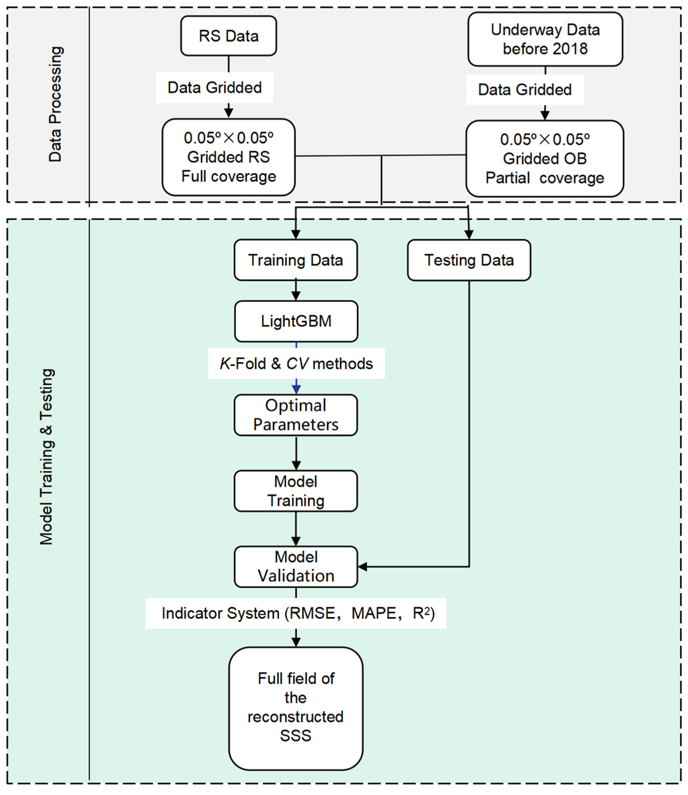
To assess the performance of our reconstruction, we calculated the biases of three global gridded SSS databases, OISSS, IAPOS, and MUL, relative to the SCS observational data and compared them with the bias of our reconstructed data. The OISSS dataset is produced by the International Pacific Research Center, University of Hawaii at Manoa, in collaboration with Remote Sensing Systems (RSS, Santa Rosa, CA, USA), with a horizontal resolution of 0.25° and is available at https://podaac.jpl.nasa.gov/ (available from 25 August 2011 to the present day, accessed on 30 August 2021). The IAPOS dataset combined ensemble optimal interpolation for the World Ocean Database data with CMIP5 model results [34]. This database has a spatial resolution of 1° × 1° and monthly resolution from 1940 to 2018 (available at https://climatedataguide.ucar.edu/, accessed on 30 August 2021). The MUL dataset, originally developed within the MyOcean project (http://www.myocean.eu.org, accessed on 30 August 2021) with satellite SST data to constrain surface salinity patterns, has been produced at a spatial resolution of 0.25° × 0.25° from 1993 to the present day in the framework of the CMEMS (available at https://resources.marine.copernicus.eu/, accessed on 30 August 2021).

3. Methods

The SSS reconstruction procedure used is shown in Figure 2. Briefly, it consists of two steps: (I) data processing, and (II) model training and testing. For data processing, we first gridded the underway observational SSS data OB_A and remote sensing data into 0.05° × 0.05° grids for any given month using a spatial average method. Then, these gridded underway SSS data and remote sensing data were grouped into seasonal datasets to set up four seasonal SSS reconstruction models. Finally, to achieve a better reconstruction of the SSS in the coastal area where more observations were available, we divided the entire SCS into two regions with the 200 m isobath as the dividing line. The data in each subregion were randomly divided into a training (85%) and a testing subset (15%), which were then combined to comprise the final training and testing sets for the entire SCS. For model training and testing, preliminary experiments were performed to calculate the optimal model parameters using K-fold and cross validation methods with the training set. Then, these optimal parameters of the LightGBM algorithm were applied to model training. Finally, the independent testing set was used to assess the performance of the SSS reconstruction models, and accuracy indicators of the reconstructed SSS were calculated. The differences between our reconstructed data and observational data were calculated using concurrent data on a monthly scale. Detailed methods are described below.

3.1. The LightGBM Algorithm

The LightGBM algorithm is a histogram-based decision tree (DT) algorithm, in which DT has a flowchart-like tree structure. In addition, this algorithm is widely used in ocean science, e.g., [35]. Each of its internal nodes represents a test on an attribute, its branch shows the outcome of the test, and the class label can be found in each leaf node [36]. It can effectively handle high-dimensional data. The histogram-based LightGBM is efficient in terms of both memory consumption and training speed and can be used in regression, classification, and other machine learning fields with speed and high-performance [36]. The code and details of LightGBM are available at https://github.com/microsoft/LightGBM (accessed on 30 August 2021).

3.2. Parameter Optimization

In the machine learning training process, K-fold and cross validation, also known as loop validation, were applied to calculate the optimal model parameters. Briefly, the original training data were subdivided into K groups (K-fold), and one group was taken as a training dataset and the remaining groups were used as validation datasets [37]. The cross-validation errors of these K models were subsequently calculated, and the optimal parameters were determined with the minimum error. The code of K-fold and cross-validation can be downloaded at https://github.com/suryanktiwari/Linear-Regression-and-K-fold-Cross-Validation (accessed on 30 August 2021).

3.3. Evaluation Metrics

Common error metrics to evaluate the accuracy of reconstructed data include the root mean square error (RMSE), mean absolute percentage error (MAPE), and coefficient of determination (R2). RMSE stands for the standard deviation of the residuals (prediction error) between the fitted line and data points calculated as:
RMSE = 1 n i = 1 n ( y i y r i ) 2
where y stands for the observational data, yr represents the reconstructed data, and n is the number of data points. MAPE is a statistical measure that uses a percentage to assess the bias between the data produced with a machine learning algorithm and the observational data. The lower the value of MAPE, the better the fit of the model. MAPE is calculated as:
MAPE = 1 n i = 1 n | y i y r i | | y i | × 100 %

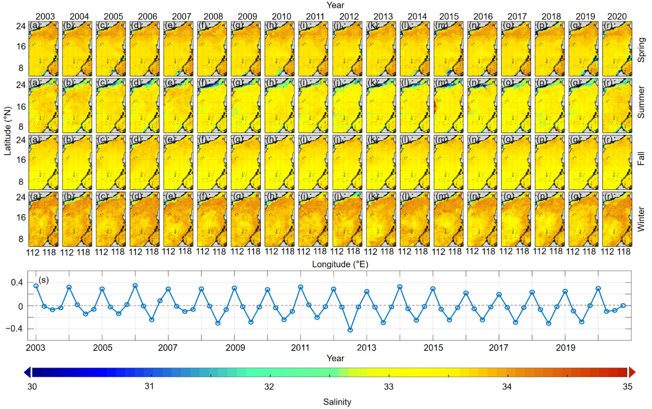
4. Results of the Reconstruction

The four seasonal training sets of reconstructed SSS data fit the observational data well (Figure 3), with an average RMSE of 0.26 and an average MAPE of 0.60%. The average R2 of the training sets is 0.92. For the testing sets, although there are some outliers, most of the reconstructed SSS is consistent with the observational data, with an average RMSE of 0.43 and an average MAPE of 0.84%. The R2 of the testing sets is the largest for the summer data, and the smallest for the fall data, with an average of 0.81. For both training and testing sets, the spring data have the lowest RMSE, while the summer data have the highest (Table 2). The greatest spatial variance in the SSS and relatively complex regional processes, such as river plumes and upwelling, resulted in the greatest error in the summer. The percent of accuracy, which is 100%-MAPE, of the four seasonal models is almost 99% for the testing set and greater than 99% for the training set. These evaluation metrics of the training and testing sets indicate that our reconstructed SSS fields have high accuracy.
Our reconstructed SSS in the SCS shows strong full-region consistency with the underway observational data (Figure 4 and Figure 5). The SSS in the SCS basin is consistent with previous studies [38,39], namely ca. 33 in summer, while in the coastal areas, the SSS shows relatively high spatial variability. Based on the observations (Figure 4), the spatial variation in the entire SCS in spring is relatively small (ranging from 0.14 to 0.77), except in the coastal area off the Pearl River Estuary (PRE), where the maximum spatial variance of the SSS is 1.72. The low salinity in the southern SCS basin in our reconstructed SSS field is mainly controlled by the river plume of Borneo Island [40,41]. In the summer, the reconstructed SSS successfully shows the spreading of the Pearl River plume on the northern shelf of the SCS and that of the Mekong River plume in the mid-basin (~112°E, 10°N as illustrated by Chen et al. [42], as well as relatively high SSS along the coast north of the PRE and the west coast of Vietnam where upwelling usually occurs in the summer [43,44,45]. The annual change in the intensity of the Pearl River plume in the summer is clearly evidenced in the reconstructed SSS field. For example, the spreading of the Pearl River plume was limited with an SSS ≤ 32 only in the estuarine area in 2011 and 2012, but in 2013, 2014, and 2016 the region of SSS ≤ 32 extended eastward on the northern shelf, indicating a stronger Pearl River plume. This result is quite consistent with the observational data of Pearl River water discharge (see http://xxfb.mwr.cn/, accessed on 30 August 2021). The highest salinity in the summers of 2015 and 2016 was due to strong Vietnam upwelling [45]. The SSS distributions in the fall and winter are comparable to that in the spring, with small basin-wide spatial variation, although in general the average SSS in the fall is lower than that in the spring. In the winter, there is a banded low SSS area on the northern SCS shelf, which is contributed to by the China Coastal Current driven by the prevailing northwest monsoon [44,46]. In general, the average SSS in the SCS attains a minimum in the summer and a maximum in the winter as illustrated by both observational and reconstructed data in Figure 5s. The seasonal SS variation in the SCS seems to be closely related to precipitation [41,47] since the latter is greatest in the summer and lowest in the winter (https://psl.noaa.gov/data/gridded/data.cmap.html, accessed on 30 August 2021) in the SCS and relevant watersheds, resulting in the greatest river discharge and direct precipitation into the SCS in the summer and the lowest in the winter. In addition, the mixed layer is relatively deep in winter (https://psl.noaa.gov/data/gridded/tables/multi.html, accessed on 30 August 2021) in the SCS, so that subsurface water masses with relatively high salinity mix upward into surface water, causing a further increase in the SSS. Thus, the spatial and temporal consistency of our reconstructed SSS throughout the SCS (Figure 5) with underway observations (Figure 4) confirms that the reconstruction is robust.
Climatological monthly and seasonal average SSS values were calculated based on the reconstructed monthly SSS over 2003–2020 (Figure 6). The spatial distribution of the climatological SSS is essentially consistent with that of the underway observations (Figure 4), especially in the areas influenced by the China Coastal Current in the winter and the Pearl River plume in the summer. The spatio-temporal distribution of the climatological fields is also consistent with the sea surface circulation (Figure 6). In the northern SCS, the reconstructed SSS fields are mainly influenced by the westward flow from the Luzon Strait and the Pearl River plume which begins to increase in September and peaks in February. As the winter monsoon begins to transition to the summer monsoon in the SCS, the westward flow from the Luzon Strait weakens, and the coast of the northern SCS is affected by an eastward flow that carries the Pearl River plume and lowers the SSS in this region. Thus, the influence of the Pearl River plume is greatest in July. Moreover, in summer, the Mekong River plume intensifies, and a northbound flow from the western SCS carries the Mekong River plume and bifurcates around 12°N, with one branch moving northward and the other flowing eastward [48]. The spatio-temporal changes of the low salinity area (SSS ≤ 33) in the western SCS are consistent with the extent of the eastward flow (Figure 6e–h), which represents the intensity of the Mekong River plume [48]. This consistency indicates that our reconstructed SSS in the western SCS relatively accurately represents the dynamic impact of the Mekong River plume in the SCS.

5. Discussion

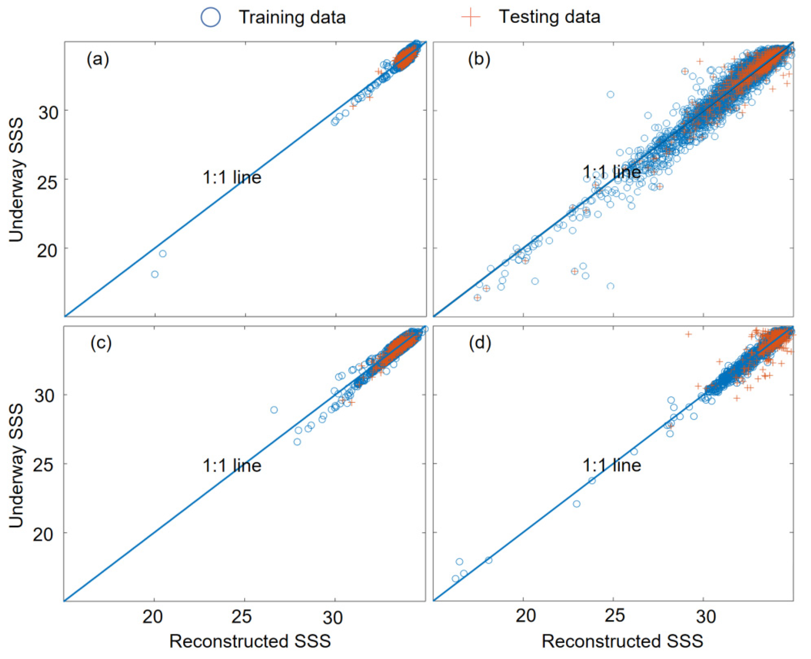
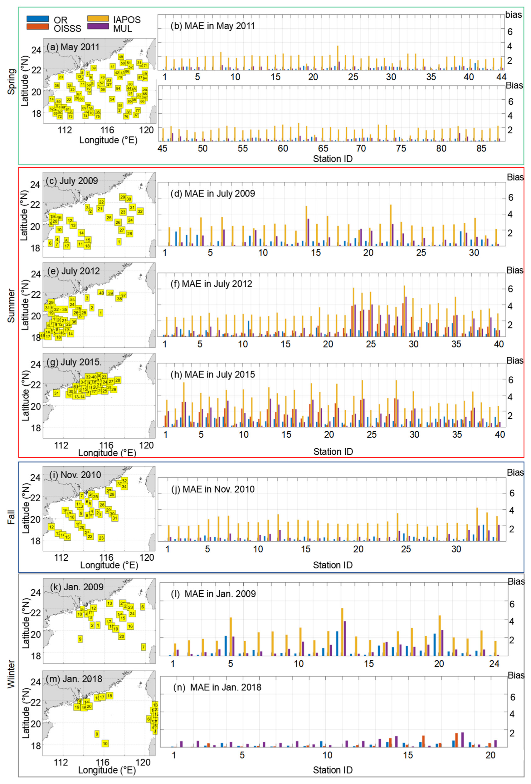
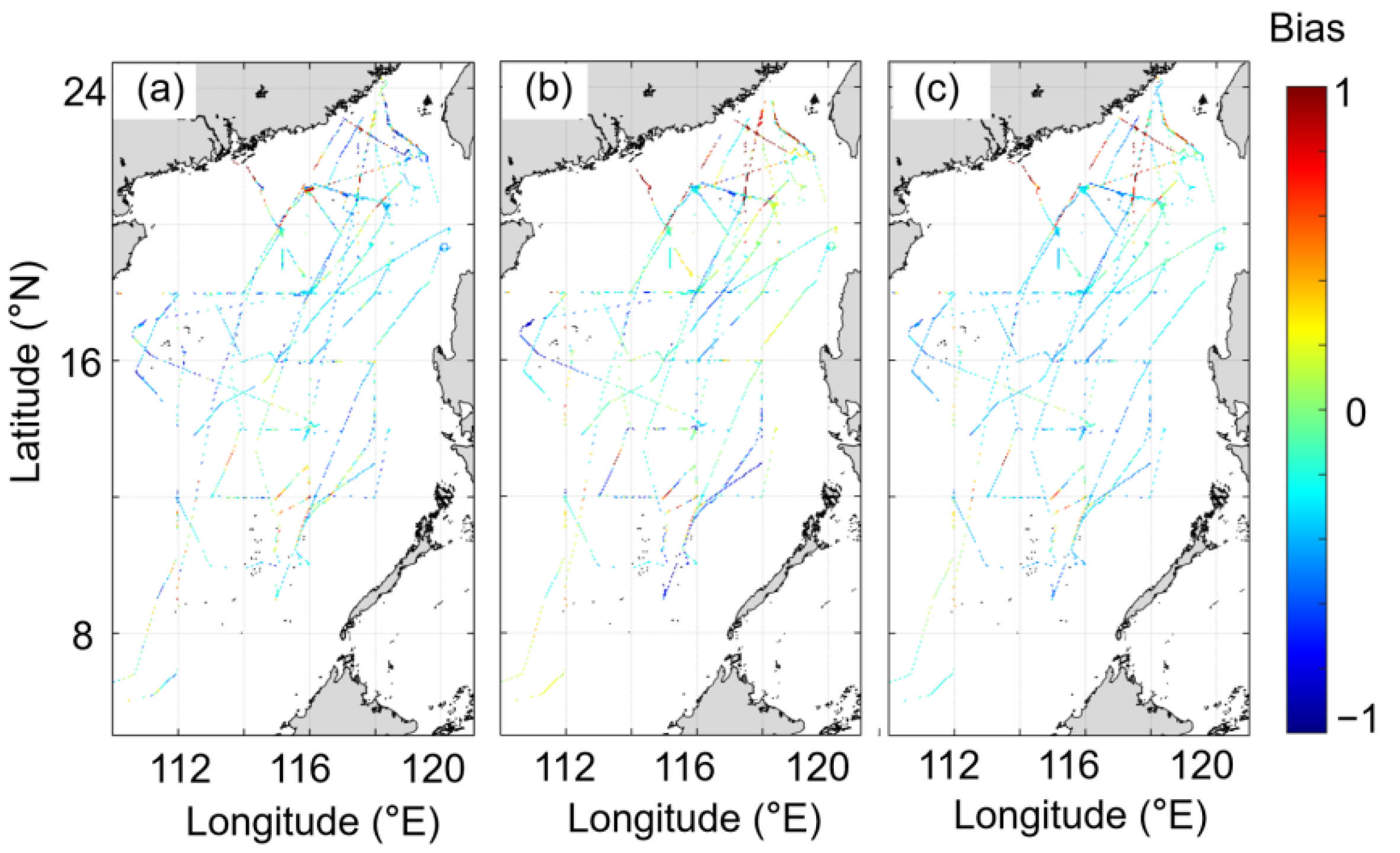
5.1. Validation and Uncertainty

Three types of observational data, the station-based data collected using CTD, SOCAT data, and the underway OB_B data, were used to validate our reconstruction results. In addition, we calculated the MAE and RMSE between the three previously mentioned model-derived datasets (OISSS, IAPOS, and MUL) and the three above mentioned types of observational datasets, as well as OB_A for comparison with our reconstructed data (Table 3). The mean absolute error (MAE) is the absolute average difference between the observations and the reconstructed data and was calculated as follows:
MAE = 1 n i n |   y i y c o m i |
where y c o m stands for the datasets used for comparison (our reconstructions, OISSS, IAPOS, and MUL).

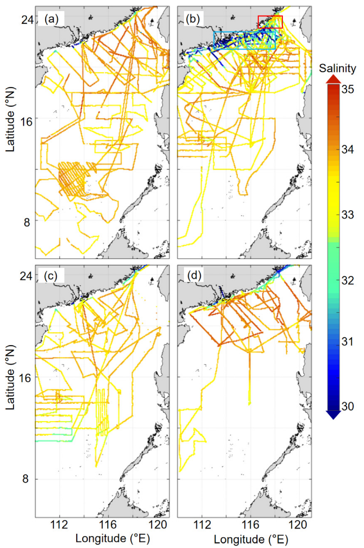
5.1.1. Comparison with the Underway Observational Data OB_A

In the spring, the difference between our reconstructed data and the underway OB_A data almost always falls within ±0.3 (Figure 7a,b) with an MAE of 0.20. The MAE between the OISSS and the underway OB_A data is 0.21, which was calculated for 2012 and 2014 when the OISSS data were available. In contrast, the MAE between our reconstructed data and the OB_A data for the same period is 0.16. The IAPOS data obviously provide overestimates in coastal waters (Figure 7d) with an MAE of 0.24, whereas the MUL data clearly provide underestimates in the SCS basin (Figure 7e) with an MAE of 0.34.
In the summer, the difference between our reconstructed data and the OB_A data almost always falls within ±0.4 (Figure 7f,g), and a relatively large differential appears in coastal areas within the 100 m isobath. Excluding this area, the MAE between our reconstructed data and the underway data is 0.12. Due to the complex conditions of coastal seawater color influenced by river plumes, upwelling, and other meso-scale processes, especially in the summer, the remote sensing data may have a relatively large bias, which can propagate to our reconstructed fields. The MAE between the OISSS and the OB_A data, which was calculated for 2012, 2015, 2016, and 2017, is 0.72. In contrast, the MAE between our reconstructed data and the OB_A data during the same period is 0.37, which is still much lower than that for the OISSS data. The IAPOS and MUL data clearly provide overestimates in coastal waters but yield underestimates in the SCS basin (Figure 7i,j). The MAE is 0.91 for the IAPOS data and 0.94 for the MUL data.
In the fall, the difference between our reconstructed data and the OB_A data generally falls within ±0.15 (Figure 7k,l), and the MAE is 0.20. The IAPOS data clearly overestimated the SSS in the SCS, especially in coastal areas, characterized by an MAE of 0.46. The MUL data overestimated the SSS off the PRE but underestimated the SSS elsewhere with an MAE of 0.38.
In the winter, the difference between our reconstructed data and the OB_A data generally falls within ±0.15 (Figure 7p,q) with an MAE of 0.15. The MAE between the OISSS and the OB_A data in 2018 is 0.21. In contrast, the MAE between our reconstructed data and the OB_A data for the same year is 0.14, which is much less than that for the OISSS. The IAPOS data obviously overestimated all of the SSS in the entire SCS, especially in coastal areas, with an MAE of 0.44. The MUL data provide overestimates of the SSS off the PRE and the west of the Luzon Strait (Figure 7t) but underestimates elsewhere, with an MAE of 0.43.

5.1.2. Comparison with the Station-Based Observational Data

When validated with the station-based data (Table 3 & Figure 8), which were independent of model training and testing, the MAE for our reconstructed data is 0.20 in the spring of 2011, the IAPOS data have the largest MAE of 1.85 among these databases, and the MAE of MUL data is 0.41. In the summer of 2009, the MAE of IAPOS data shows the largest bias among these databases (Table 3), and the MAE of our reconstructed data is 0.62. In the summer of 2012, the bias of our reconstructed data is relatively large at stations near the east coast of Hainan Island (MAE: 0.84, RMSE: 0.97, Figure 8) where the SSS is often affected by summer upwelling [49,50]. Therefore, our reconstructed data have some limitations in their ability to simulate the SSS in this region. However, compared with the three other model-derived databases, reconstructed data still show the highest overall performance (MAE: 0.59, RMSE: 0.78). In the summer of 2015, the bias of these databases decreases with the distance from the PRE. In the fall of 2012, the IAPOS data show the largest bias in both MAE and RMSE among these databases, with both being around 2.5. The MAE of our reconstructed data is 0.34 with a relatively large bias in the coastal area. In the winter of 2009, the IAPOS data show the largest bias among these databases, i.e., ~3 for both MAE and RMSE, while that of the reconstructed data in the winters of 2009 and 2018 is relatively small for both MAE and RMSE, indicating that our reconstructed data are relatively accurate in winter. Because of the limitation of the spatial coverage of station-based observational data, the southern basin of SCS needs further testing.

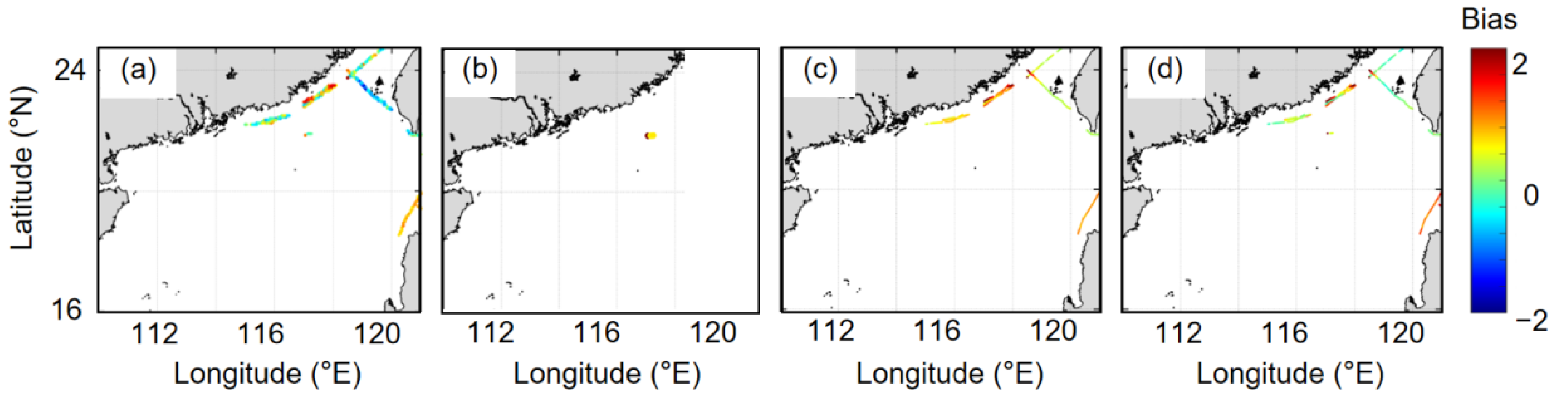
5.1.3. Comparison with the Underway Data from SOCAT and OB_B

In addition to the station-based data, we selected two other underway datasets for independent validation. One is the SOCAT underway dataset. Although the SOCAT data available in the study domain were in the coastal area, our reconstructions still show relatively high accuracy with an MAE of 0.30 and RMSE of 0.35 (Figure 9, Table 3). The three other model-derived databases overestimated the SSS with a larger MAE and RMSE (MAE: 0.82 and RMSE: 0.96 for OISSS, 0.76 and 0.77 for IAPOS, and 0.86 and 1.34 for MUL) than our reconstructed data. The second underway dataset is OB_B, corresponding to the observational data collected after 2018. The RMSEs of the other model-derived databases (OISSS and MUL) are similar (~1.25), while our reconstructed data show relatively high accuracy with an RMSE of 0.64 (Figure 10, Table 3).
These results indicate that SSS was successfully reconstructed in the SCS, and that the reconstructed data were more accurate than the other SSS data products currently available both in the basin and coastal areas. Greater biases, however, were present between our reconstructed data and the station-based observational data than those between the former and the underway data in coastal regions, which is due to the fact that the station-based SSS data were not measured SSS values, but rather the depth-average salinity of the surface 5 m. Besides that, the coastal area is too dynamic. The station-based data and the underway data are not completely matched (sampled at different times), as the reconstructions are based on the underway data, so they are more comparable to the underway data. Thus, additional biases may result from the station-based SSS data in the coastal regions, especially in upwelling-influenced areas, while this may not be the case in the SCS basin.

5.1.4. Advantages and Disadvantages of Our Method Compared with Existing Methods

OISSS is able to retrieve the salinity in near real time, however the salinity data are only available starting from 2011. IAPOS is a data product consistent with some physical processes and biogeochemical cycles, but its inversion capability in the SCS is relatively poor. MUL has slightly lower accuracy than the OISSS data but is available starting from 1998. A general disadvantage of the three global products is their relatively low spatial resolution (0.25° × 0.25°) and relatively high bias in the SCS (Table 3). Our method yields high accuracy and reasonable spatial patterns. The disadvantage of our method is that no physical/biogeochemical mechanisms are considered, an intrinsic drawback of the machine learning algorithm.

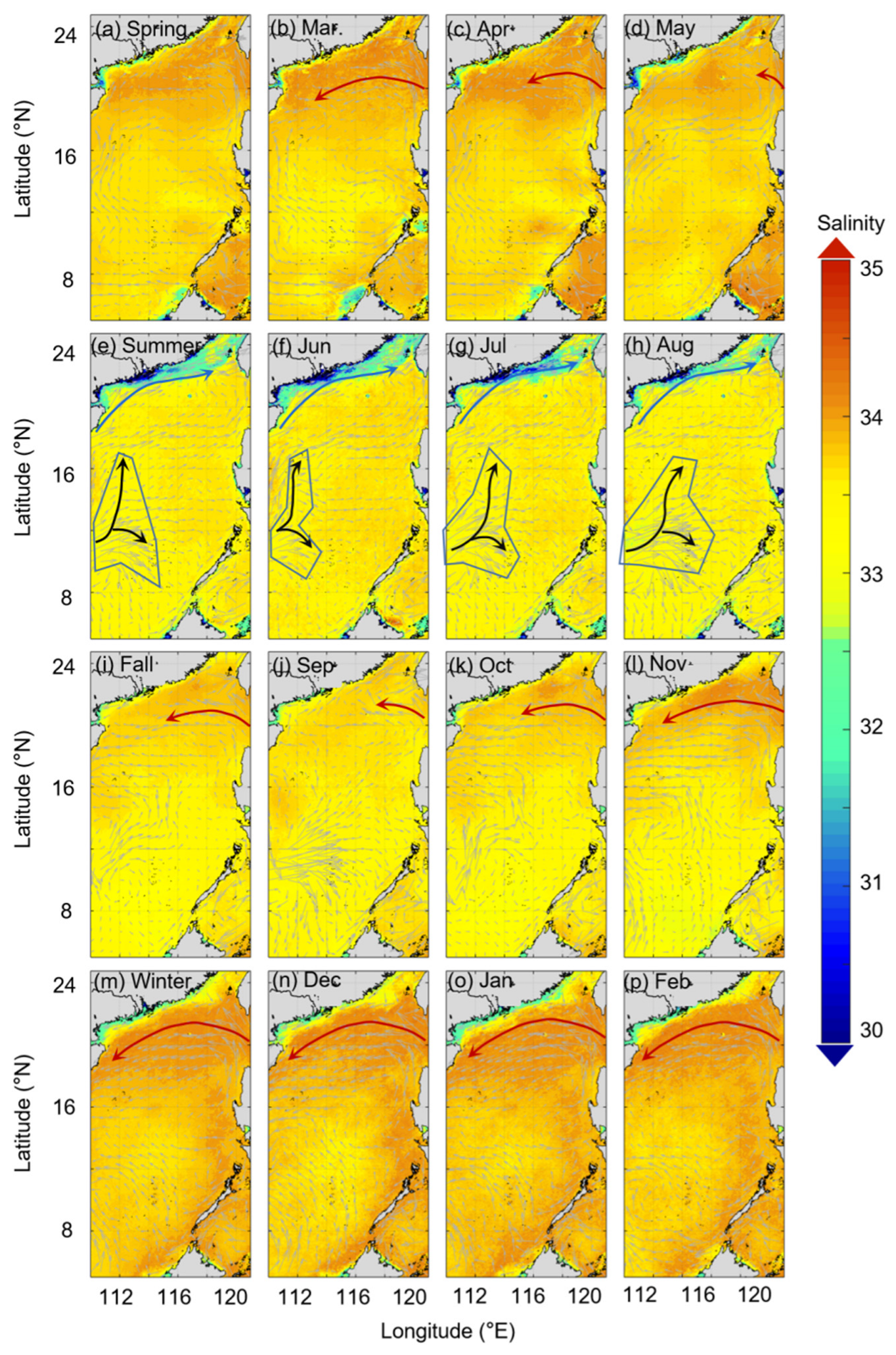
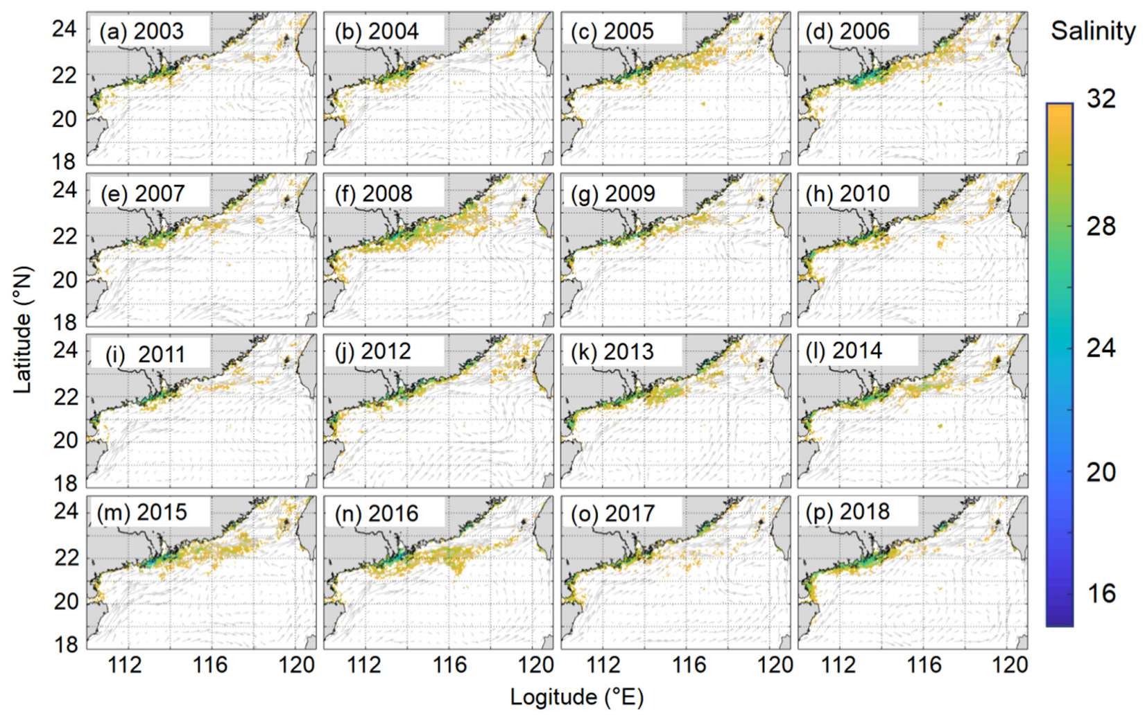
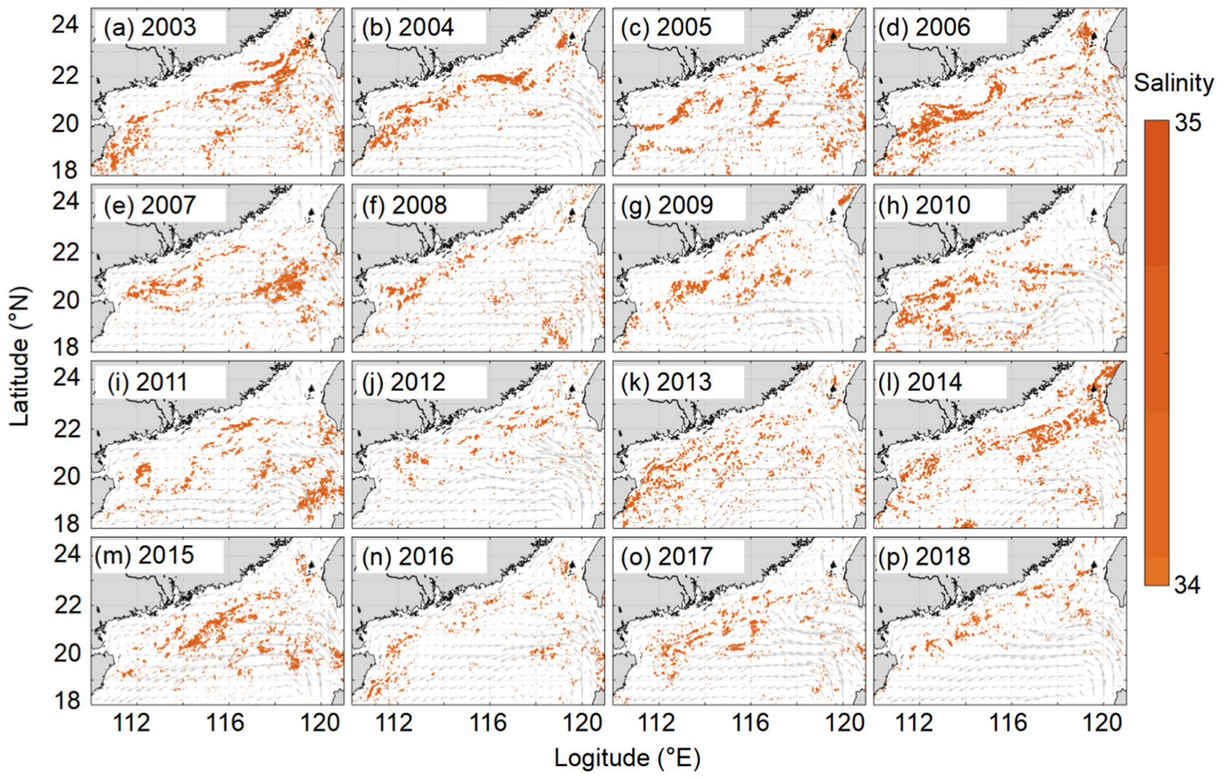
5.2. Application of the Reconstructed SSS Field in the SCS

The spatial variation of the SSS in the northern SCS is mainly controlled by two processes: the spread of the Pearl River plume and intrusion of the Kuroshio Current [44]. Due to limited temporal and spatial coverage of observational SSS data, it is difficult to resolve continuous temporal changes in the intensity of these two processes in the SCS. Here, we took advantage of the high-resolution reconstructed SSS field and defined two indices to assess the strength of the two processes in the SCS. Since the river discharge data of the Pearl River are available from 2005–2018 (http://xxfb.mwr.cn/, accessed on 30 August 2021), the discussion in this section is focused on the period before 2019.

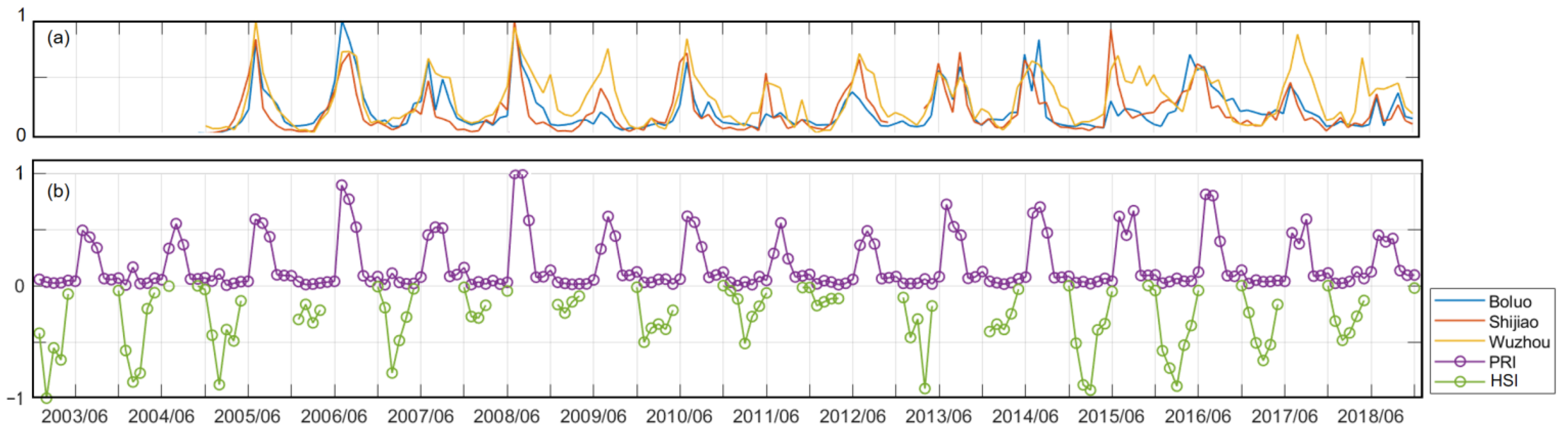
5.2.1. The Pearl River Plume Index

The reconstructed SSS field generated in this study demonstrates that the summer spatial distribution of the Pearl River plume over 2003–2018 on the northern shelf and slope of the SCS exhibits the minimum SSS off the estuary and a pattern of increasing SSS with increasing distance offshore (Figure 11). In addition, the plume water spreads mainly eastward in summer, which is consistent with the known sea surface circulation.
A Pearl River plume index (PRI) was thus set up using the reconstructed SSS to indicate the intensity of the Pearl River plume in the SCS. To avoid the potential noise of other water masses with relatively low SSS, e.g., the China Coastal Current in the winter in the PRI, we used the Pearson correlation coefficient [51] between the Pearl River discharge and SSS with a significance level of 5% to determine the area influenced by the Pearl River plume as follows:
Pearson   Correlation   Coefficient   =   Σ [ ( y r i y r ¯ ) × ( P r i P r ¯ ) ]   /   ( σ y r × σ P r )
where Pr is the Pearl River discharge, σ y r is the standard deviation of y r , and σ P r is the standard deviation of P r . We calculated this coefficient grid-by-grid and determined the Pearl River plume-influenced area. We then calculated the PRI, as:
PRI   = ( 35 S S S _ P R ¯ ) × N s 32
where S S S _ P R ¯ represents the average salinity in the Pearl River plume-influenced area and Ns32 indicates the number of grids with salinity ≤32 in this area.
The PRI reflects not only the area influenced by the river plume, but also the plume intensity. We calculated the monthly change in the river discharge of the three tributaries of the Pearl River (Station Wuzhou (111.27°E, 23.48°N), Station Shijiao (113.52°E, 23.86°N), and Station Boluo (114.28°E, 23.17°N) representing the West River, North River and East River for the north tributary of the Pearl River, respectively. The maximum monthly PRI over a year represents the yearly strongest plume in the northern SCS, which co-occurs with the yearly greatest river discharges of the three main Pearl River tributaries (Figure 12). This co-occurrence indicates that the PRI provides a good index of the plume intensity, which is directly related to the river discharge. It further verifies the accuracy of our reconstructed SSS data. Furthermore, combining the PRI with the relative river discharges of the three tributaries, allows us to readily determine which tributary is the main controller of the Pearl River plume in a given month.

5.2.2. The Sea Surface High Salinity Index

The Kuroshio Current, characterized by high salinity, usually shows the greatest intrusion in the SCS in winter [44,52,53], leading to a relatively high surface salinity (SSS ≥ 34.25) in the northern SCS. The intrusion of the Kuroshio water is thus a notable forcing factor in the northern SCS. In this study, to better illustrate the impact of Kuroshio intrusion water on the SSS, as well as the association between the high SSS water mass and sea surface circulation, we described the spatial distribution of relatively high SSS (≥34.25) in the winter based on our reconstructed SSS data in the northern SCS. The latter could successfully characterize the SSS changes caused by the Kuroshio intrusion (Figure 13).
Wu et al. [54] used the sea surface height anomaly (SSHA, 15–20°N, 114–120°E) to define the timing of the Kuroshio intrusion. When the SSHA is anomalously high (SSHA > 0), the Kuroshio intrusion will hardly occur. As with the PRI, we thus defined an index to characterize the effect of the Kuroshio intrusion and water mass with high salinity on the SSS in the northern SCS, namely the sea surface high salinity index (HSI):
HIS = SSHA × NS34.25
where Ns≥34.25 is the number of grids with SSS ≥ 34.25 in the northern SCS (18–25°N, 109–122°E). The strength of the Kuroshio intrusion is related to its flow velocity, and the SSHA indicates the speed and direction of sea surface circulation in the SCS (Wu et al. [54]). Thus, this formula considers both the strength of the Kuroshio intrusion and the changes in SSS. The more negative the HSI, the stronger the effect of the Kuroshio intrusion on the SSS.
The SSHA was designated as NAN when the Kuroshio intrusion did not occur. Thus, the HSI was calculated only in months when the Kuroshio intrusion occurred. Our results indicate that this index clearly shows the Kuroshio intrusion starting in the fall, shows it intensifying in early winter, and weakening in late winter. When no Kuroshio intrusion occurs, the northern SCS is often affected by the Pearl River plume. The two indices, PRI and HSI, demonstrate that the northern SCS is mainly under the alternating forcing of the Kuroshio intrusion and the Pearl River plume, a finding which is consistent with the results of previous studies (Yang et al. [44]). Therefore, these two indices provide an effective, quantitative tool to evaluate the intensity of the two processes in the northern SCS in any given month, and thus serve to further increase the usefulness of our reconstructed SSS data.

6. Conclusions

Based on the LightGBM machine learning method, we reconstructed the SSS fields by calculating the statistical relationship between the underway observational SSS data and remote sensing data. The reconstructed data successfully displayed the SSS spatio-temporal patterns in the SCS with a high spatial resolution (0.05° × 0.05°) over the last two decades (2003–2020).
We used multiple observational datasets, underway observations, station-based observations, and SOCAT data, in the validation of our reconstructed fields and current open-source, model-derived SSS datasets (OISSS, IAPOS, and MUL) in the SCS. The results of these independent validation datasets show that our reconstruction data are at least 50% (from Table 3) more accurate than the three other model-derived databases (OISSS, IAPOS, and MUL) in the SCS. The average bias of the OISSS, IAPOS, or MUL is small at a global scale, but for the SCS, especially in the coastal area, the bias increases considerably. The MAE/RMSE of our reconstructed data in the SCS is relatively small (0.42/0.58), whereas the maximum bias of our reconstructed data occurs off the PRE on the northern shelf of the SCS in the summer, and the accuracy of our reconstruction increases with the distance offshore. These validations verify the robustness of our reconstruction.
In general, our reconstructed SSS is consistent with the spatial and temporal patterns of the observations and successfully reflects the spread of the Pearl River plume and Kuroshio intrusion in the northern SCS. Based on our reconstructed SSS, two new indices, the RPI and the HSI, were developed that successfully quantified the relative intensity of the two most notable forcings in the northern SCS, the Pearl River plume and the Kuroshio intrusion.

Author Contributions

M.D. conceptualized and directed the field program of in situ observations. X.G. and J.H. participated in the in situ data collection. G.W., M.D. and Z.W. developed the reconstruction method, analyzed the data, and wrote the original manuscript. Z.W. wrote the code and plotted the figures. All the authors contributed to the editing and revisions of the manuscript. All authors have read and agreed to the published version of the manuscript.

Funding

This work is supported by the National Natural Science Foundation of China (Grant No. 42141001, 42188102, 418908004, 4218810291958203 and 41730533) and by the National Basic Research Program of China (Grant No. 2015CB954004 and 2009CB421208).

Data Availability Statement

The reconstructed SSS data for this paper are openly and freely available at Science Data Bank under the link: https://doi.org/10.57760/sciencedb.02053.

Conflicts of Interest

The authors declare no conflict to interest.

References

  1. Holliday, N.; Hughes, S.; Shammon, T.; Sherwin, T. Scientific review-ocean salinity. In Marine Climate Change Impacts Annual Report Card 2008; MCCIP: Lowestoft, UK, 2008. [Google Scholar]
  2. Schmitt, R.W. Salinity and the global water cycle. Oceanography 2008, 21, 12–19. [Google Scholar] [CrossRef]
  3. Du, Y.; Zhang, Y.; Shi, J. Relationship between sea surface salinity and ocean circulation and climate change. Sci. China Earth Sci. 2019, 62, 771–782. [Google Scholar] [CrossRef]
  4. Wang, G.; Xie, S.P.; Qu, T.; Huang, R.X. Deep South China Sea circulation. Geophys. Res. Lett. 2011, 38, L05601. [Google Scholar] [CrossRef] [Green Version]
  5. Droghei, R.; Nardelli, B.B.; Santoleri, R. Combining in situ and satellite observations to retrieve salinity and density at the ocean surface. J. Atmos. Ocean. Technol. 2016, 33, 1211–1223. [Google Scholar] [CrossRef]
  6. Li, Q.; Guo, X.; Zhai, W.; Xu, Y.; Dai, M. Partial pressure of CO2 and air-sea CO2 fluxes in the South China Sea: Synthesis of an 18-year dataset. Prog. Oceanogr. 2020, 182, 1022–1043. [Google Scholar] [CrossRef]
  7. Umbert, M.; Hoareau, N.; Turiel, A.; Ballabrera-Poy, J. New blending algorithm to synergize ocean variables: The case of SMOS sea surface salinity maps. Remote Sens. Environ. 2014, 146, 172–187. [Google Scholar] [CrossRef]
  8. Zhao, J.; Marouane, T.; Hosni, G. Remotely sensed sea surface salinity in the hyper-saline Arabian Gulf: Application to landsat 8 OLI data. Estuarine. Coast. Shelf Sci. 2017, 187, 168–177. [Google Scholar] [CrossRef] [Green Version]
  9. Qian, Y.; Zhao, Y.; Wu, Q.-l.; Yang, Y. Review of salinity measurement technology based on optical fiber sensor. Sens. Actuators B: Chem. 2018, 260, 86–105. [Google Scholar] [CrossRef]
  10. Vinogradova, N.; Lee, T.; Boutin, J.; Drushka, K.; Fournier, S.; Sabia, R.; Stammer, D.; Bayler, E.; Reul, N.; Gordon, A. Satellite salinity observing system: Recent discoveries and the way forward. Front. Mar. Sci. 2019, 6, 243. [Google Scholar] [CrossRef] [Green Version]
  11. Klein, L.; Swift, C. An improved model for the dielectric constantof Sea water at microwave frequencies. IEEE Transactions. Antennas Propag. AP 1997, 25, 104–111. [Google Scholar] [CrossRef]
  12. Le Vine, D.M.; Abraham, S.; Wentz, F.; Lagerloef, G.S. Impact of the Sun on remote sensing of sea surface salinity from space. In Proceedings of the 2005 IEEE International Geoscience and Remote Sensing Symposium, Seoul, Korea, 29 July 2005. [Google Scholar]
  13. Le Vine, D.M.; Lagerloef, G.S.; Colomb, F.R.; Yueh, S.H.; Pellerano, F.A. Aquarius: An instrument to monitor sea surface salinity from space. IEEE Trans. Geosci. Remote Sens. 2007, 45, 2040–2050. [Google Scholar] [CrossRef]
  14. Reul, N.; Tenerelli, J.; Chapron, B.; Waldteufel, P. Modeling sun glitter at L-band for sea surface salinity remote sensing with SMOS. IEEE Trans. Geosci. Remote Sens. 2007, 45, 2073–2087. [Google Scholar] [CrossRef]
  15. Reul, N.; Tenerelli, J.E.; Floury, N.; Chapron, B. Earth-viewing L-band radiometer sensing of sea surface scattered celestial sky radiation—Part II: Application to SMOS. IEEE Trans. Geosci. Remote Sens. 2008, 46, 675–688. [Google Scholar] [CrossRef]
  16. Qing, S.; Zhang, J.; Cui, T.; Bao, Y. Retrieval of sea surface salinity with MERIS and MODIS data in the Bohai Sea. Remote Sens. Environ. 2013, 136, 117–125. [Google Scholar] [CrossRef]
  17. Geiger, E.; Grossi, M.; Trembanis, A.; Kohut, J.; Oliver. Satellite-derived coastal ocean and estuarine salinity in the Mid-Atlantic. Cont. Shelf Res. 2013, 63, 235–243. [Google Scholar] [CrossRef] [Green Version]
  18. Moussa, H.; Benallal, M.A.; Goyet, C.; Lefèvre, N.; Jai, M.E.; Guglielmi, V.; Touratier, F. A comparison of Multiple Non-linear regression and neural network techniques for sea surface salinity estimation in the tropical Atlantic Ocean based on satellite data. ESAIM: Proc. Surv. 2015, 49, 65–77. [Google Scholar] [CrossRef] [Green Version]
  19. Martínez, J.; Gabarró, C.; Turiel, A.; González-Gambau, V.; Umbert, M.; Hoareau, N.; González-Haro, C.; Olmedo, E.; Arias, M.; Catany, R.; et al. Improved BEC SMOS Arctic Sea Surface Salinity product v3.1. Earth Syst. Sci. Data 2022, 14, 307–323. [Google Scholar] [CrossRef]
  20. Chen, S.; Hu, C. Estimating sea surface salinity in the northern Gulf of Mexico from satellite ocean color measurements. Remote Sens. Environ. 2017, 201, 115–132. [Google Scholar] [CrossRef]
  21. Mu, Z.; Zhang, W.; Wang, P.; Wang, H.; Yang, X. Assimilation of SMOS sea surface salinity in the regional ocean model for South China Sea. Remote Sens. 2019, 11, 919. [Google Scholar] [CrossRef] [Green Version]
  22. Bai, Y.; Pan, D.; Cai, W.J.; He, X.; Wang, D.; Tao, B.; Zhu, Q. Remote sensing of salinity from satellite-derived CDOM in the Changjiang River dominated East China Sea. J. Geophys. Res. Ocean. 2013, 118, 227–243. [Google Scholar] [CrossRef]
  23. Du, C.; Gan, J.; Hui, C.R.; Lu, Z.; Zhao, X.; Roberts, E.; Dai, M. Dynamics of dissolved inorganic carbon in the South China Sea: A modeling study. Prog. Oceanogr. 2020, 186, 102367. [Google Scholar] [CrossRef]
  24. Lu, Z.; Gan, J.; Dai, M.; Zhao, X.; Hui, C.R. Nutrient transport and dynamics in the South China Sea: A modeling study. Prog. Oceanogr. 2020, 183, 102308. [Google Scholar] [CrossRef]
  25. Han, A.; Gan, J.; Dai, M.; Lu, Z.; Liang, L.; Zhao, X. Intensification of downslope nutrient transport and associated biological responses over the northeastern South China Sea during wind-driven downwelling: A modeling study. Front. Mar. Sci. 2021, 8, 2296–7745. [Google Scholar] [CrossRef]
  26. Lu, Y.; Wen, Z.; Shi, D.; Lin, W.; Bonnet, S.; Dai, M.; Kao, S.J. Biogeography of N2 fixation influenced by the western boundary current intrusion in the South China Sea. J. Geophys. Res. Ocean. 2019, 124, 6983–6996. [Google Scholar] [CrossRef] [Green Version]
  27. Meng, F.; Dai, M.; Cao, Z.; Wu, K.; Zhao, X.; Li, X.; Chen, J.; Gan, J. Seasonal dynamics of dissolved organic carbon under complex circulation schemes on a large continental shelf: The Northern South China Sea. J. Geophys. Res. Ocean. 2017, 122, 9415–9428. [Google Scholar] [CrossRef] [Green Version]
  28. Barreiro, M.; Fedorov, A.; Pacanowski, R.; Philander, S.G. Abrupt climate changes: How freshening of the northern Atlantic affects the thermohaline and wind-driven oceanic circulations. Annu. Rev. Earth Planet. Sci. 2008, 36, 35–58. [Google Scholar] [CrossRef] [Green Version]
  29. Sen, A.; Caruso, D.; Lagerloef, G.; Torrusio, S.; Durham, D.; Falcon, C. Aquarius/SAC-D mission, Sensors, Systems, and Next-Generation Satellites XII. Int. Soc. Opt. Eng. 2008, 5. [Google Scholar] [CrossRef]
  30. Entekhabi, D.; Njoku, E.G.; O’Neill, P.E.; Kellogg, K.H.; Crow, W.T.; Edelstein, W.N.; Entin, J.K.; Goodman, S.D.; Jackson, T.J.; Johnson, J. The soil moisture active passive (SMAP) mission. Proc. IEEE 2010, 98, 704–716. [Google Scholar] [CrossRef]
  31. Crapolicchio, R.; Ferrazzoli, P.; Meloni, M.; Pinori, S.; Rahmoune, R. Soil Moisture and Ocean Salinity (SMOS) mission: System overview and contribution to vicarious calibration monitoring. Riv. Ital. Telerilevamento 2010, 42, 37–50. [Google Scholar] [CrossRef]
  32. Melnichenko, O.; Hacker, P.; Maximenko, N.; Lagerloef, G.; Potemra, J. Spatial optimal interpolation of Aquarius sea surface salinity: Algorithms and implementation in the North Atlantic. J. Atmos. Ocean. Technol. 2014, 31, 1583–1600. [Google Scholar] [CrossRef]
  33. Melnichenko, O.; Hacker, P.; Maximenko, N.; Lagerloef, G.; Potemra, J. Optimum interpolation analysis of Aquarius sea surface salinity. J. Geophys. Res. Ocean 2016, 121, 602–616. [Google Scholar] [CrossRef] [Green Version]
  34. Cheng, L.; Trenberth, K.E.; Gruber, N.; Abraham, J.P.; Fasullo, J.T.; Li, G.; Mann, M.E.; Zhao, X.; Zhu, J. Improved estimates of changes in upper ocean salinity and the hydrological cycle. J. Clim. 2020, 33, 10357–10381. [Google Scholar] [CrossRef]
  35. Gan, M.; Pan, S.; Chen, Y.; Cheng, C.; Pan, H.; Zhu, X. Application of the Machine Learning LightGBM Model to the Prediction of the Water Levels of the Lower Columbia River. J. Mar. Sci. Eng 2021, 9, 496. [Google Scholar] [CrossRef]
  36. Ke, G.; Meng, Q.; Finley, T.; Wang, T.; Chen, W.; Ma, W.; Ye, Q.; Liu, T.-Y. Lightgbm: A highly efficient gradient boosting decision tree. Adv. Neural Inf. Process. Syst. 2017, 30, 3146–3154. [Google Scholar]
  37. Refaeilzadeh, P.; Tang, L.; Liu, H. Cross-validation. In Encyclopedia of Database Systems; Springer: Berlin/Heidelberg, Germany, 2009; Volume 5, pp. 532–538. [Google Scholar]
  38. Qi, J.; Liu, C.; Chi, J.; Li, D.; Gao, L.; Yin, B. An Ensemble-Based Machine Learning Model for Estimation of Subsurface Thermal Structure in the South China Sea. Remote Sens. 2022, 14, 3207. [Google Scholar] [CrossRef]
  39. Zeng, L.; Wang, D.; Chen, J.; Wang, W.; Chen, R. SCSPOD14, A South China Sea physical oceanographic dataset derived from in situ measurements during 1919–2014. Sci. Data 2016, 3, 160029. [Google Scholar] [CrossRef] [Green Version]
  40. Tarya, A.; Hoitink, A.; Van der Vegt, M.; van Katwijk, M.; Hoeksema, B.; Bouma, T.; Lamers, L.; Christianen, M. Exposure of coastal ecosystems to river plume spreading across a near-equatorial continental shelf. Cont. Shelf Res. 2018, 153, 1–15. [Google Scholar] [CrossRef]
  41. Tian, J.; Wang, P.; Cheng, X. Development of the East Asian monsoon and Northern Hemisphere glaciation: Oxygen isotope records from the South China Sea. Quat. Sci. Rev. 2004, 23, 2007–2016. [Google Scholar] [CrossRef]
  42. Chen, W.; Liu, Q.; Huh, C.A.; Dai, M.; Miao, Y.C. Signature of the Mekong River plume in the western South China Sea revealed by radium isotopes. J. Geophys. Res. Ocean 2010, 115, 1023–1025. [Google Scholar] [CrossRef] [Green Version]
  43. Gan, J.; Wang, J.; Liang, L.; Li, L.; Guo, X. A modeling study of the formation, maintenance, and relaxation of upwelling circulation on the Northeastern South China Sea shelf. Deep Sea Res. Part II Top. Stud. Oceanogr. 2015, 117, 41–52. [Google Scholar] [CrossRef]
  44. Yang, W.; Guo, X.; Cao, Z.; Wang, L.; Guo, L.; Huang, T.; Li, Y.; Xu, Y.; Gan, J.; Dai, M. Seasonal dynamics of the carbonate system under complex circulation schemes on a large continental shelf: The northern South China Sea. Prog. Oceanogr. 2021, 197, 1026–1045. [Google Scholar] [CrossRef]
  45. Wu, H.; Deng, B.; Yuan, R.; Hu, J.; Gu, J.; Shen, F.; Zhu, J.; Zhang, J. Detiding measurement on transport of the Changjiang-derived buoyant coastal current. J. Phys. Oceanogr. 2013, 43, 2388–2399. [Google Scholar] [CrossRef]
  46. Kuo, N.; Zheng, Q.; Ho, C. Response of Vietnam coastal upwelling to the 1997–1998 ENSO event observed by multi-sensor data. Remote Sens. Environ. 2004, 89, 106–115. [Google Scholar] [CrossRef]
  47. Steinke, S.; Chiu, H.-Y.; Yu, P.-S.; Shen, C.-C.; Erlenkeuser, H.; Löwemark, L.; Chen, M.-T. On the influence of sea level and monsoon climate on the southern South China Sea freshwater budget over the last 22,000 years. Quat. Sci. Rev. 2006, 25, 1475–1488. [Google Scholar] [CrossRef]
  48. Zeng, X.; Bracco, A.; Tagklis, F. Dynamical impact of the Mekong River plume in the South China Sea. J. Geophys. Res. Ocean. 2022, 127, 1029–1044. [Google Scholar] [CrossRef]
  49. Lin, P.; Cheng, P.; Gan, J.; Hu, J. Dynamics of wind-driven upwelling off the northeastern coast of Hainan Island. J. Geophys. Res. Ocean 2016, 121, 1160–1173. [Google Scholar] [CrossRef]
  50. Lin, P.; Hu, J.; Zheng, Q.; Sun, Z.; Zhu, J. Observation of summertime upwelling off the eastern and northeastern coasts of Hainan Island. China. Ocean Dynam 2016, 66, 387–399. [Google Scholar] [CrossRef]
  51. Benesty, J.; Chen, J.; Huang, Y.; Cohen, I. Pearson correlation coefficient. In Noise Reduction in Speech Processing; Springer: Berlin/Heidelberg, Germany, 2009; pp. 1–4. [Google Scholar]
  52. Du, C.; Liu, Z.; Dai, M.; Kao, S.-J.; Cao, Z.; Zhang, Y.; Huang, T.; Wang, L.; Li, Y. Impact of the Kuroshio intrusion on the nutrient inventory in the upper northern South China Sea: Insights from an isopycnal mixing model. Biogeosciences 2013, 10, 6419–6432. [Google Scholar] [CrossRef] [Green Version]
  53. Park, J.H.; Farmer, D. Effects of Kuroshio intrusions on nonlinear internal waves in the South China Sea during winter. J. Geophys. Res. Ocean 2013, 118, 7081–7094. [Google Scholar] [CrossRef]
  54. Wu, C. Interannual modulation of the pacific decadal oscillation (PDO) on the low-latitude western north pacific. Prog. Oceanogr. 2013, 110, 49–58. [Google Scholar] [CrossRef]
Figure 1. Frequency of sea surface salinity (SSS) in the South China Sea during four seasons from October 2003 to September 2020 ((a). Spring; (b). Summer; (c). Fall; (d). Winter).
Remotesensing 14 06147 g001
Figure 2. Procedure for the reconstruction of sea surface salinity (SSS) using machine learning; RS represent remote sensing data and OB observational data; CV indicates cross validation, RMSE represents the root mean square error, MAPE represents the mean absolute percentage error, and R2 represents the coefficient of determination.
Remotesensing 14 06147 g002
Figure 3. Relationship between the reconstructed sea surface salinity (SSS) and the underway observations OB_A for training and testing data ((a). Spring; (b). Summer; (c). Fall; (d). Winter).
Remotesensing 14 06147 g003
Figure 4. Distribution of temporally averaged underway sea surface salinity (SSS) in the South China Sea during four seasons. The green box in panel b indicates the area influenced by the Pearl River plume, and the red box indicates the area influenced by coastal upwelling. The data sources are listed in Table 1 ((a). Spring; (b). Summer; (c). Fall; (d). Winter).
Remotesensing 14 06147 g004
Figure 5. Reconstructed seasonal sea surface salinity (SSS) fields in the South China Sea during 2003–2020 (ar) and seasonal anomalies of SSS during 2003–2020 (s).
Remotesensing 14 06147 g005
Figure 6. Seasonal and monthly reconstructed sea surface salinity (SSS) fields averaged over 2003–2020 in the South China Sea. Light grey arrows indicate sea surface circulation; red arrows represent the surface direction and extent of the westward flow from the Luzon Strait; black arrows represent the surface direction and extent of the eastward flow from the western and mid-SCS; and blue arrows represent the surface direction and extent of the coastal current in the northern SCS. The blue box is the low salinity area (SSS ≤ 33) influenced by the Mekong River plume. The surface circulation data are from https://resources.marine.copernicus.eu/ (accessed on 30 August 2021).
Remotesensing 14 06147 g006
Figure 7. Difference between the model-derived sea surface salinity (SSS) data and concurrent observational underway OB_A data in four seasons. The black dashed line represents the 100 m isobath. The first column (a,f,k,p) shows the results of the reconstructed data for the training dataset, the second column (b,g,l,q) shows the results of the reconstructed data for the testing dataset, the third column (c,h,m,r) shows the results of OISSS, the fourth column (d,i,n,s) shows the results of IAPOS, and the fifth column (e,j,o,t) shows the results of MUL (see the main text for abbreviations). The observational data source is listed in Table 1. The OISSS data are only available after 2011; no observational fall data are available after 2011. Thus, the results of OISSS in the fall (m) are left blank.
Remotesensing 14 06147 g007
Figure 8. Difference between the model-derived sea surface salinity (SSS) data (OR: our reconstructed data, OISSS, IAPOS, and MUL) and concurrent station-based observational data (a,c,e,g,i,k,m): observation stations in four seasons; (b,d,f,h,j,l,n): corresponding MAE). The OISSS data are available only after 2011.
Remotesensing 14 06147 g008
Figure 9. Difference between the model-derived sea surface salinity (SSS) data and concurrent SOCAT underway SSS data. (a) Reconstructed data (OR), (b) OISSS, (c) IAPOS, and (d) MUL. The SOCAT data were collected in September 2008, April 2009, and January 2018; the OISSS data were available in January 2018.
Remotesensing 14 06147 g009
Figure 10. Difference between the model-derived sea surface salinity (SSS) data and concurrent underway OB_B data. (a) Reconstructed data generated in the present study, (b) OISSS, and (c) MUL. The IAPOS data are only available from 1940 to 2018 and were not used in this comparison.
Remotesensing 14 06147 g010
Figure 11. Spatial distributions of low sea surface salinity, SSS (SSS ≤ 32) and surface circulation in the summer during 2003–2018 in the northern South China Sea. The SSS is our reconstructed data; surface circulation data are from https://resources.marine.copernicus.eu/ (accessed on 30 August 2021).
Remotesensing 14 06147 g011
Figure 12. Relative river discharges of the three tributaries of the Pearl River and the standardized monthly Pearl River plume index (PRI) and sea surface high salinity index (HSI) in the northern South China Sea over 2003–2018. (a) Relative river discharges, in which Station Boluo represents the East River, Station Shijiao stands for the North River, and Station Wuzhou represents the West River, and (b) temporal changes in the standardized monthly PRI and HSI in the northern SCS. The HSI is not shown where there is no Kuroshio intrusion, i.e., SSS < 34.25.
Remotesensing 14 06147 g012
Figure 13. Spatial distribution of relatively high sea surface salinity (SSS ≥ 34.25) and sea surface circulation in the winter in the northern South China Sea from 2003 to 2018. The SSS represents our reconstructed data; surface circulation data are from https://resources.marine.copernicus.eu/ (accessed on 30 August 2021).
Remotesensing 14 06147 g013
Table 1. Seasonal underway sea surface salinity (SSS) data in the South China Sea compiled in this study.
SeasonCruise TimeData Source
SpringMarchAprilMayLi et al. (2020) [6]
* This study
2004.032005.042004.05
2008.042011.05
2009.042014.05
2012.042020.05 *
2020.04 *
SummerJuneJulyAugust
2006.06 *2004.072007.08
2016.062005.07 *2008.08
2017.06 *2007.072019.08 *
2019.06 *2008.07
2020.06 *2009.07
2012.07
2015.07 *
2019.07 *
FallSeptemberOctoberNovember
2004.092003.102006.11
2007.092006.102010.11
2008.09
2020.09 *
WinterDecemberJanuaryFebruary
2006.122009.012004.02
2010.012006.02
2018.01
Table 2. Evaluation metrics, root mean square error (RMSE), coefficient of determination (R2), and mean absolute percentage error (MAPE) of the sea surface salinity reconstruction.
SeasonRMSE_TrainRMSE_TestR2_TrainR2_TestMAPE_Train
(%)
MAPE_Test
(%)
Spring0.200.210.890.820.490.51
Summer0.450.690.940.870.931.13
Fall0.230.260.900.750.590.66
Winter0.180.580.970.810.421.06
Table 3. The mean absolute error (MAE) and root mean square error (RMSE) compared between the model-derived data and concurrent observational data.
This ReconstructionOISSSIAPOSMUL
SpringUnderway
OB_A data
MAE0.200.210.240.34
RMSE0.360.240.320.41
Station-based Data in 2011.05MAE0.20NAN1.850.37
RMSE0.27NAN1.890.42
SummerUnderway
OB_A data
MAE0.340.720.910.94
RMSE0.660.750.951.06
Station-based Data in 2009.07MAE0.62NAN2.770.94
RMSE0.80NAN2.891.26
Station-based Data in 2012.07MAE0.591.153.391.25
RMSE0.781.543.571.76
Station-based Data in 2015.07MAE0.841.353.611.67
RMSE0.911.683.781.91
FallUnderway
OB_A data
MAE0.20NAN0.460.38
RMSE0.23NAN0.520.44
Station-based Data in 2010.11MAE0.34NAN2.520.65
RMSE0.51NAN2.580.85
WinterUnderway
OB_A data
MAE0.150.210.440.43
RMSE0.250.330.530.48
Station-based Data in 2009.01MAE0.57NAN2.921.21
RMSE0.75NAN3.862.36
Station-based Data in 2012.01MAE0.310.86NAN0.85
RMSE0.391.31NAN1.18
Underway OB_B data MAE0.400.52NAN0.58
RMSE0.641.13NAN1.46
SOCAT dataMAE0.300.820.760.86
RMSE0.350.960.771.34
Publisher’s Note: MDPI stays neutral with regard to jurisdictional claims in published maps and institutional affiliations.

