

Coupling an Ecological Network with Multi-Scenario Land Use Simulation: An Ecological Spatial Constraint Approach
 , , , ,
Abstract

1. Introduction
2. Study Area and Datasets
2.1. Study Area
2.2. Datasets
3. Methodology
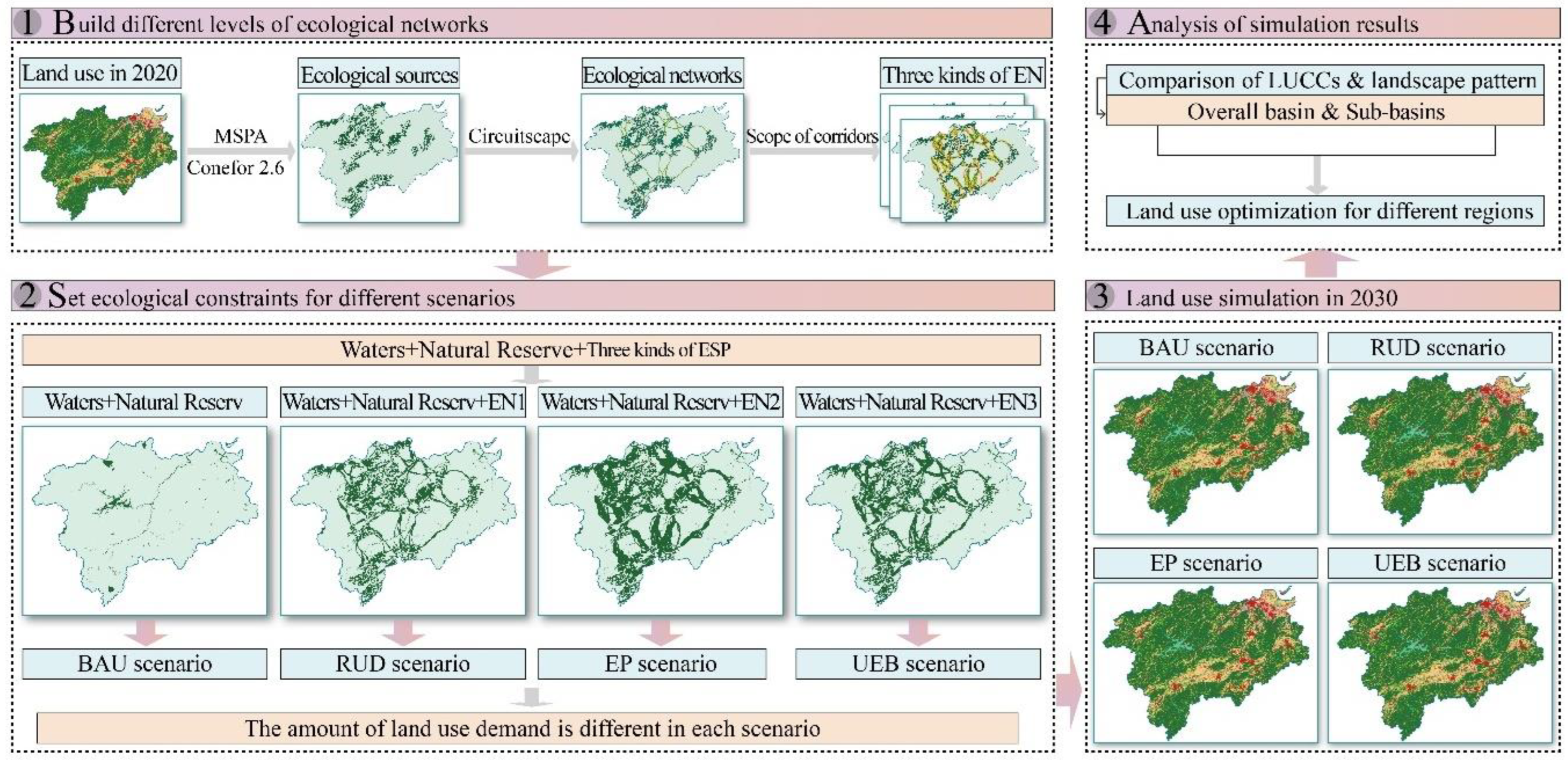
3.1. Design of the EN-PLUS Model
3.2. Constructing the Ecological Network
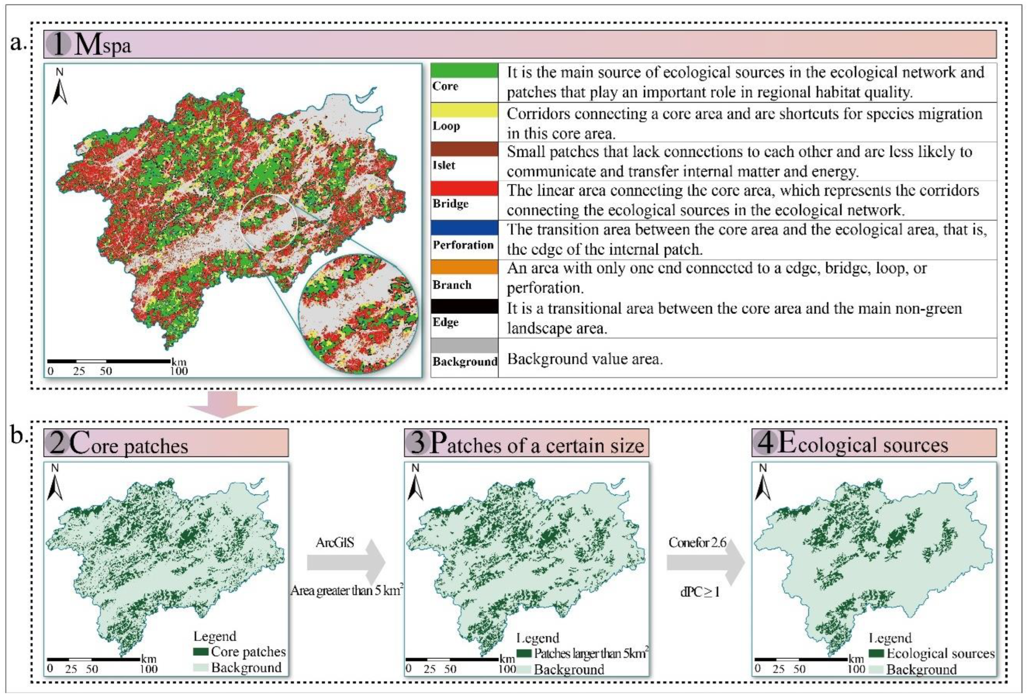
3.2.1. Identifying of Ecological Sources
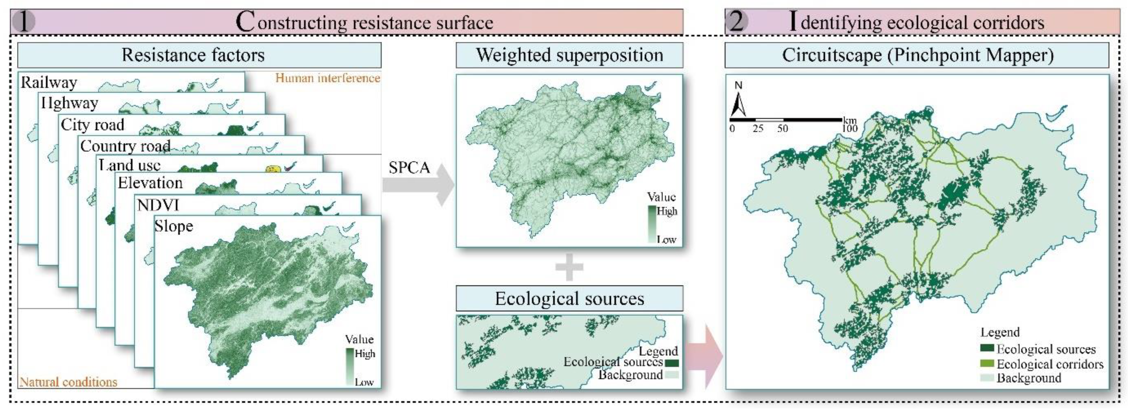
3.2.2. Mapping the Ecological Resistance Surface and Identifying the Ecological Corridor
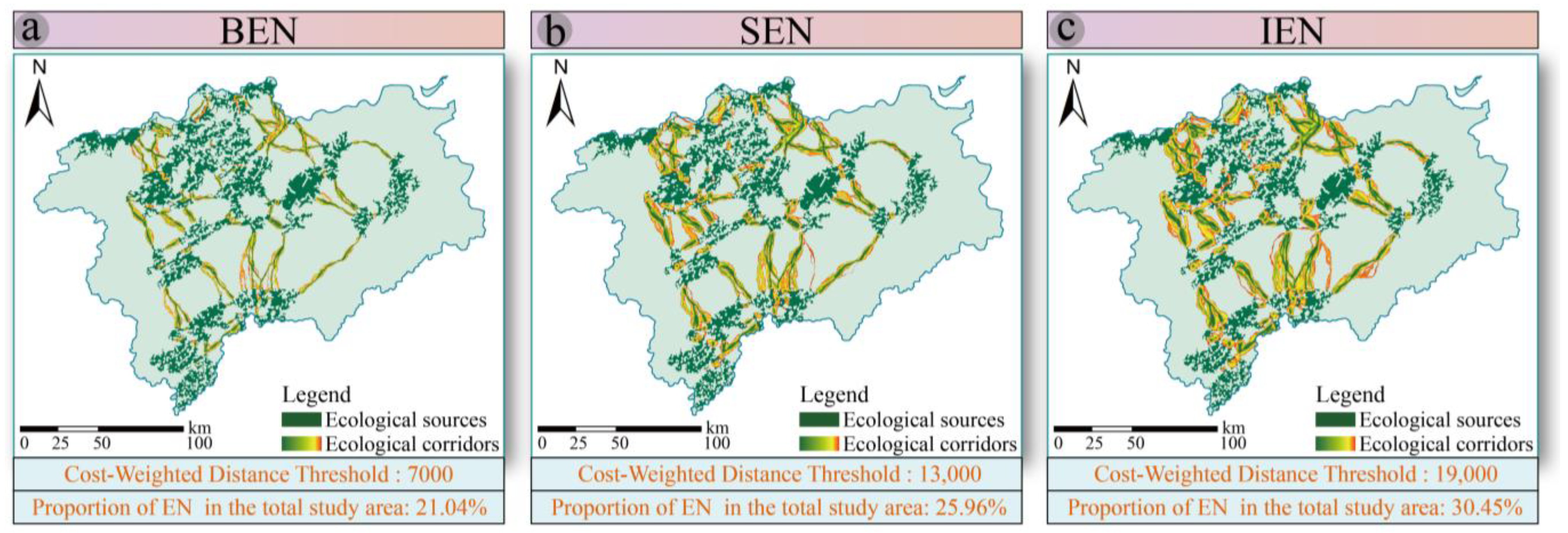
3.2.3. Three Types of ENs Serving as Ecologically Constrained Space
3.3. Four Scenarios for Regional Development
- BAU scenario: In this scenario, the trend of land use change is consistent with that in the past 10 years.
- RUD scenario: In this scenario, the scale of urban expansion and the intensity of human development are greater than before. Therefore, the probability of converting nonconstruction land into urban construction land increases by 20%, and the probability of converting it into rural construction land and industrial land increases by 10%. The probability of converting construction land to other land use is reduced by 30%, and the probability of converting rural construction land to the other two types of construction land is increased by 20%.
- EP scenario: This scenario emphasizes protecting the environment and reducing urban expansion. Therefore, the probability of converting cultivated land and woodland into construction land is reduced by 30%. The probability of converting waters, grassland, and unused land into construction land is reduced by 20%. In addition, the probability of converting construction land into cultivated land, woodland, and grassland is increased by 20%, and the probability of converting rural construction land into other construction land types is decreased by 20%.
- UEB scenario: This scenario requires the coordination of ecological protection and urban development. In terms of ecological protection, the probability of converting cultivated land and woodland into construction land is reduced by 15% and the probability of converting waters and grassland into construction land is reduced by 10%. In terms of urban development, the expansion probability of rural construction land in the RUD scenario is reserved. In addition, the probability of converting construction land into other land is decreased by 15%, and the probability of converting unused land into construction land is increased by 10%.
3.4. Land Use Simulation Model—PLUS
3.4.1. PLUS Model Settings—Driving Factors Required for the LEAS Module
3.4.2. PLUS Model Settings—Cost Matrix and Neighborhood Weight Required for the CARS Module
3.5. Landscape Pattern Analysis of Each Scenario
4. Results
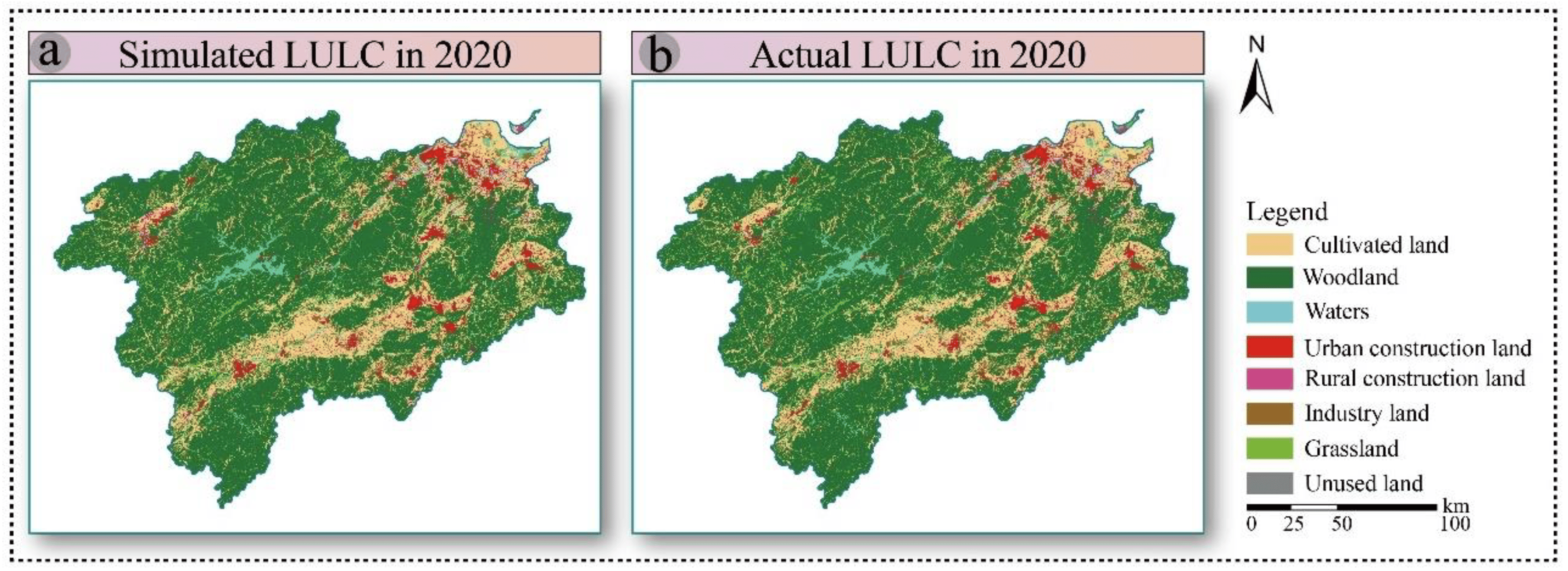
4.1. Validation
4.2. Land Use Quantity and Layout in Each Scenario
4.2.1. Analysis at the Whole Basin Scale
4.2.2. Analysis at the Subbasins Scale
4.3. Scenario Comparison Using the Landscape Pattern Index
5. Discussion
5.1. Matching Degree between the EN-PLUS Model and the Preset Scenarios
5.2. Land Use Optimization Modeling Oriented to Ecological Land Protection
5.3. Scale Dependence of Simulation Results
5.4. Limitations and Future Research Directions
6. Conclusions
- The four ecological constraints in the EN-PLUS model play different roles in the protection of ecological land. This protective effect is more pronounced under the EP and UEB scenarios, while under the RUD scenario, the extent of ecological pattern destruction is still greater than that under the BAU scenario due to excessive human disturbance.
- The simulation results showed obvious landscape scale effects at subbasins scale.
- Although the damage to the landscape pattern is generally lower under the EP scenario, it is not the best development scenario for all subbasins. The scale effect and the regional ecological characteristics should be comprehensively considered to select the best regional development scenario.
Supplementary Materials
Author Contributions
Funding
Conflicts of Interest
References
- Weilin, W.; Jiao, L.; Jia, Q.; Liu, J.; Mao, W.; Xu, Z.; Li, W. Land Use Optimization Modelling with Ecological Priority Perspective for Large-Scale Spatial Planning. Sustain. Cities Soc. 2021, 65, 102575. [Google Scholar]
- Luca, S.; Zambon, I.; Chelli, F.M.; Serra, P. Do Spatial Patterns of Urbanization and Land Consumption Reflect Different Socioeconomic Contexts in Europe? Sci. Total Environ. 2018, 625, 722–730. [Google Scholar]
- Wenbin, N.; Yang, F.; Xu, B.; Bao, Z.; Shi, Y.; Liu, B.; Wu, R.; Lin, W. Spatiotemporal Evolution of Landscape Patterns and Their Driving Forces under Optimal Granularity and the Extent at the County and the Environmental Functional Regional Scales. Front. Ecol. Evol. 2022, 10, 954232. [Google Scholar]
- Wenbin, N.; Shi, Y.; Siaw, M.J.; Yang, F.; Wu, R.; Wu, X.; Zheng, X.; Bao, Z. Constructing and Optimizing Ecological Network at County and Town Scale: The Case of Anji County, China. Ecol. Indic. 2021, 132, 108294. [Google Scholar]
- Jayne, T.S.; Chamberlin, J.; Headey, D.D. Land Pressures, the Evolution of Farming Systems, and Development Strategies in Africa: A Synthesis. Food Policy 2014, 48, 1–17. [Google Scholar] [CrossRef]
- Eugenia, K.; Cai, M. Impact of Urbanization and Land-Use Change on Climate. Nature 2003, 423, 528–531. [Google Scholar]
- Liu, H.; Gong, P.; Wang, J.; Wang, X.; Ning, G.; Xu, B. Production of Global Daily Seamless Data Cubes and Quantification of Global Land Cover Change from 1985 to 2020-Imap World 1.0. Remote Sens. Environ. 2021, 258, 112364. [Google Scholar] [CrossRef]
- David, T.; Fargione, J.; Wolff, B.; D’antonio, C.; Dobson, A.; Howarth, R.; Schindler, D.; Schlesinger, W.H.; Simberloff, D.; Swackhamer, D. Forecasting Agriculturally Driven Global Environmental Change. Science 2001, 292, 281–284. [Google Scholar]
- United Nations. World Urbanization Prospects: The 2014 Revision, Highlights; Department of Economic and Social Affairs; Population Division; United Nations: New York, NY, USA, 2014. [Google Scholar]
- Vera, H.; Hoff, H.; Wirsenius, S.; Meyer, C.; Kreft, H. Land Use Options for Staying within the Planetary Boundaries–Synergies and Trade-Offs between Global and Local Sustainability Goals. Glob. Environ. Chang. 2018, 49, 73–84. [Google Scholar]
- Wenbin, N.; Xu, B.; Yang, F.; Shi, Y.; Liu, B.; Wu, R.; Lin, W.; Hui, P.; Bao, Z. Simulating Future Land Use by Coupling Ecological Security Patterns and Multiple Scenarios. Sci. Total Environ. 2023, 859, 160262. [Google Scholar]
- Groot, J.C.J.; Yalew, S.G.; Rossing, W.A.H. Exploring Ecosystem Services Trade-Offs in Agricultural Landscapes with a Multi-Objective Programming Approach. Landsc. Urban Plan. 2018, 172, 29–36. [Google Scholar] [CrossRef]
- Mengyu, J.; Hu, M.; Xia, B. Spatiotemporal Dynamic Simulation of Land-Use and Landscape-Pattern in the Pearl River Delta, China. Sustain. Cities Soc. 2019, 49, 101581. [Google Scholar]
- Courage, K.; Aniya, M.; Adi, B.; Manjoro, M. Rural Sustainability under Threat in Zimbabwe–Simulation of Future Land Use/Cover Changes in the Bindura District Based on the Markov-Cellular Automata Model. Appl. Geogr. 2009, 29, 435–447. [Google Scholar]
- Genga, B.; Zhengb, X.Q.; Fua, M.C. Scenario Analysis of Sustainable Intensive Land Use Based on Sd Model. Sustain. Cities Soc. 2017, 29, 193–202. [Google Scholar] [CrossRef]
- Liang, Z.; Dang, X.; Sun, Q.; Wang, S. Multi-Scenario Simulation of Urban Land Change in Shanghai by Random Forest and Ca-Markov Model. Sustain. Cities Soc. 2020, 55, 102045. [Google Scholar]
- Clarke, K.C.; Hoppen, S.; Gaydos, L. A Self-Modifying Cellular Automaton Model of Historical Urbanization in the San Francisco Bay Area. Environ. Plan. B Plan. Des. 1997, 24, 247–261. [Google Scholar] [CrossRef]
- Aburas, M.M.; Ho, Y.M.; Ramli, M.F.; Ash’aari, Z.H. Improving the Capability of an Integrated Ca-Markov Model to Simulate Spatio-Temporal Urban Growth Trends Using an Analytical Hierarchy Process and Frequency Ratio. Int. J. Appl. Earth Obs. Geoinf. 2017, 59, 65–78. [Google Scholar] [CrossRef]
- Fei, F.; Deng, S.; Wu, D.; Liu, W.; Bai, Z. Research on the Spatiotemporal Evolution of Land Use Landscape Pattern in a County Area Based on Ca-Markov Model. Sustain. Cities Soc. 2022, 80, 103760. [Google Scholar]
- Chen, G.Z.; Li, X.; Liu, X.P.; Chen, Y.M.; Liang, X.; Leng, J.Y.; Xu, X.C.; Liao, W.L.; Qiu, Y.A.; Wu, L.Q.; et al. Global Projections of Future Urban Land Expansion under Shared Socioeconomic Pathways. Nat. Commun. 2020, 11, 1–12. [Google Scholar] [CrossRef]
- Verburg, P.H.; Soepboer, W.; Veldkamp, A.; Limpiada, R.; Espaldon, V.; Mastura, S.S.A. Modeling the Spatial Dynamics of Regional Land Use: The Clue-S Model. Environ. Manag. 2002, 30, 391–405. [Google Scholar] [CrossRef]
- Daquan, H.; Huang, J.; Liu, T. Delimiting Urban Growth Boundaries Using the Clue-S Model with Village Administrative Boundaries. Land Use Policy 2019, 82, 422–435. [Google Scholar]
- Xiaoping, L.; Liang, X.; Li, X.; Xu, X.; Ou, J.; Chen, Y.; Li, S.; Wang, S.; Pei, F. A Future Land Use Simulation Model (Flus) for Simulating Multiple Land Use Scenarios by Coupling Human and Natural Effects. Landsc. Urban Plan. 2017, 168, 94–116. [Google Scholar]
- Zhou, Y.; Jiang, C.; Shan-Shan, F. Effects of Urban Growth Boundaries on Urban Spatial Structural and Ecological Functional Optimization in the Jining Metropolitan Area, China. Land Use Policy 2022, 117, 106113. [Google Scholar]
- Xun, L.; Guan, Q.; Clarke, K.C.; Liu, S.; Wang, B.; Yao, Y. Understanding the Drivers of Sustainable Land Expansion Using a Patch-Generating Land Use Simulation (Plus) Model: A Case Study in Wuhan, China. Comput. Environ. Urban Syst. 2021, 85, 101569. [Google Scholar]
- Zhou, F.; Ding, T.; Chen, J.; Xue, S.; Zhou, Q.; Wang, Y.; Wang, Y.; Huang, Z.; Yang, S. Impacts of Land Use/Land Cover Changes on Ecosystem Services in Ecologically Fragile Regions. Sci. Total Environ. 2022, 831, 154967. [Google Scholar]
- Yonghua, L.; Ma, Q.; Song, Y.; Han, H. Bringing Conservation Priorities into Urban Growth Simulation: An Integrated Model and Applied Case Study of Hangzhou, China. Resour. Conserv. Recycl. 2019, 140, 324–337. [Google Scholar]
- Xie, H.L.; Zhu, Z.H.; He, Y.F. Regulation Simulation of Land-Use Ecological Security, Based on a Ca Model and Gis: A Case-Study in Xingguo County, China. Land Degrad. Dev. 2022, 33, 1564–1578. [Google Scholar] [CrossRef]
- Marcus, S.; Mattone, C.; Connolly, R.M.; Hernandez, S.; Nagelkerken, I.; Murray, N.; Ronan, M.; Waltham, N.J.; Bradley, M. Ecological Constraint Mapping: Understanding Outcome-Limiting Bottlenecks for Improved Environmental Decision-Making in Marine and Coastal Environments. Front. Mar. Sci. 2021, 8, 717448. [Google Scholar] [CrossRef]
- Pengju, L.; Hu, Y.; Jia, W. Land Use Optimization Research Based on Flus Model and Ecosystem Services–Setting Jinan City as an Example. Urban Clim. 2021, 40, 100984. [Google Scholar]
- Emmett, B.A.; Cooper, D.; Smart, S.; Jackson, B.; Thomas, A.; Cosby, B.; Evans, C.; Glanville, H.; McDonald, J.E.; Malham, S.K.; et al. Spatial Patterns and Environmental Constraints on Ecosystem Services at a Catchment Scale. Sci. Total Environ. 2016, 572, 1586–1600. [Google Scholar] [CrossRef]
- Peng, J.; Yang, Y.; Liu, Y.; Hu, Y.; Du, Y.; Meersmans, J.; Qiu, S. Linking Ecosystem Services and Circuit Theory to Identify Ecological Security Patterns. Sci. Total Environ. 2018, 644, 781–790. [Google Scholar] [CrossRef] [PubMed]
- Paul, O.; Steingröver, E.; van Rooij, S. Ecological Networks: A Spatial Concept for Multi-Actor Planning of Sustainable Landscapes. Landsc. Urban Plan. 2006, 75, 322–332. [Google Scholar]
- Ahern, J. Planning for an Extensive Open Space System: Linking Landscape Structure and Function. Landsc. Urban Plan. 1991, 21, 131–145. [Google Scholar] [CrossRef]
- Lu, Y.H.; Li, T.; Whitham, C.; Feng, X.M.; Fu, B.J.; Zeng, Y.; Wu, B.F.; Hu, J. Scale and Landscape Features Matter for Understanding the Performance of Large Payments for Ecosystem Services. Landsc. Urban Plan. 2020, 197, 103764. [Google Scholar] [CrossRef]
- Knaapen, J.P.; Scheffer, M.; Harms, B. Estimating Habitat Isolation in Landscape Planning. Landsc. Urban Plan. 1992, 23, 1–16. [Google Scholar] [CrossRef]
- McRae, B.H.; Beier, P. Circuit Theory Predicts Gene Flow in Plant and Animal Populations. Proc. Natl. Acad. Sci. USA 2007, 104, 19885–19890. [Google Scholar] [CrossRef]
- Huang, L.Y.; Wang, J.; Fang, Y.; Zhai, T.L.; Cheng, H. An Integrated Approach Towards Spatial Identification of Restored and Conserved Priority Areas of Ecological Network for Implementation Planning in Metropolitan Region. Sustain. Cities Soc. 2021, 69, 102865. [Google Scholar] [CrossRef]
- Ma, B.B.; Chen, Z.A.; Wei, X.J.; Li, X.Q.; Zhang, L.T. Comparative Ecological Network Pattern Analysis: A Case of Nanchang. Environ. Sci. Pollut. Res. 2022, 29, 37423–37434. [Google Scholar] [CrossRef]
- Yi, A.; Liu, S.; Sun, Y.; Shi, F.; Beazley, R. Construction and Optimization of an Ecological Network Based on Morphological Spatial Pattern Analysis and Circuit Theory. Landsc. Ecol. 2020, 36, 2059–2076. [Google Scholar]
- Xueqi, L.; Liu, Y.; Wang, Y.; Liu, Z. Evaluating Potential Impacts of Land Use Changes on Water Supply–Demand under Multiple Development Scenarios in Dryland Region. J. Hydrol. 2022, 610, 127811. [Google Scholar]
- Zhang, H.X.; Liao, L.; Zhai, T.L. Evaluation of Ecosystem Service Based on Scenario Simulation of Land Use in Yunnan Province. Phys. Chem. Earth 2018, 104, 58–65. [Google Scholar] [CrossRef]
- Wang, H.J.; Bao, C. Scenario Modeling of Ecological Security Index Using System Dynamics in Beijing-Tianjin-Hebei Urban Agglomeration. Ecol. Indic. 2021, 125, 107613. [Google Scholar] [CrossRef]
- Zihan, X.; Peng, J.; Dong, J.; Liu, Y.; Liu, Q.; Lyu, D.; Qiao, R.; Zhang, Z. Spatial Correlation between the Changes of Ecosystem Service Supply and Demand: An Ecological Zoning Approach. Landsc. Urban Plan. 2022, 217, 104285. [Google Scholar]
- Zeng, L.; Li, J.; Qin, K.Y.; Liu, J.Y.; Zhou, Z.X.; Zhang, Y.M. The Total Suitability of Water Yield and Carbon Sequestration under Multi-Scenario Simulations in the Weihe Watershed, China. Environ. Sci. Pollut. Res. 2020, 27, 22461–22475. [Google Scholar] [CrossRef]
- Kis, A.; Pongracz, R.; Bartholy, J.; Gocic, M.; Milanovic, M.; Trajkovic, S. Multi-Scenario and Multi-Model Ensemble of Regional Climate Change Projections for the Plain Areas of the Pannonian Basin. Idojaras 2020, 124, 157–190. [Google Scholar] [CrossRef]
- Huizhong, L.; Fang, C.; Xia, Y.; Liu, Z.; Wang, W. Multi-Scenario Simulation of Production-Living-Ecological Space in the Poyang Lake Area Based on Remote Sensing and Rf-Markov-Flus Model. Remote Sens. 2022, 14, 2830. [Google Scholar]
- Silvio, S.; Perrings, C. Bundling Ecosystem Services in the Panama Canal Watershed. Proc. Natl. Acad. Sci. USA 2013, 110, 9326–9331. [Google Scholar]
- Cheng, L.; Dengyun, W.; Wen, J.; Honghua, L.; Xiangmin, Z. Geomorphic Evolution of the Qiantang River Drainage Basin Based on the Analysis of Topographic Indexs. Quat. Sci. 2017, 37, 343–352. [Google Scholar]
- Weilin, W.; Jiao, L.; Dong, T.; Xu, Z.; Xu, G. Simulating Urban Dynamics by Coupling Top-Down and Bottom-up Strategies. Int. J. Geogr. Inf. Sci. 2019, 33, 2259–2283. [Google Scholar]
- Zhou, M.M.; Deng, J.S.; Lin, Y.; Zhang, L.J.; He, S.; Yang, W. Evaluating Combined Effects of Socio-Economic Development and Ecological Conservation Policies on Sediment Retention Service in the Qiantang River Basin, China. J. Clean. Prod. 2021, 286, 124961. [Google Scholar] [CrossRef]
- Ling, X.; Wang, H.; Liu, S. The Ecosystem Service Values Simulation and Driving Force Analysis Based on Land Use/Land Cover: A Case Study in Inland Rivers in Arid Areas of the Aksu River Basin, China. Ecol. Indic. 2022, 138, 108828. [Google Scholar]
- Jian, P.; Zhao, M.; Guo, X.; Pan, Y.; Liu, Y. Spatial-Temporal Dynamics and Associated Driving Forces of Urban Ecological Land: A Case Study in Shenzhen City, China. Habitat Int. 2017, 60, 81–90. [Google Scholar]
- Wu, A.C.; Zhou, G.Y.; He, H.L.; Hautier, Y.; Tang, X.L.; Liu, J.X.; Zhang, Q.M.; Wang, S.L.; Wang, A.Z.; Lin, L.X.; et al. Tree Diversity Depending on Environmental Gradients Promotes Biomass Stability Via Species Asynchrony in China’s Forest Ecosystems. Ecol. Indic. 2022, 140, 109021. [Google Scholar] [CrossRef]
- Mikel, G.; Lozano, P.J.; del Barrio, G. Gis-Based Approach for Incorporating the Connectivity of Ecological Networks into Regional Planning. J. Nat. Conserv. 2010, 18, 318–326. [Google Scholar]
- Yu, K. Security Patterns and Surface Model in Landscape Ecological Planning. Landsc. Urban Plan. 1996, 36, 1–17. [Google Scholar] [CrossRef]
- Santiago, S.; Vogt, P.; Velázquez, J.; Hernando, A.; Tejera, R. Key Structural Forest Connectors Can Be Identified by Combining Landscape Spatial Pattern and Network Analyses. For. Ecol. Manag. 2011, 262, 150–160. [Google Scholar]
- Vogt, P.; Ferrari, J.R.; Lookingbill, T.R.; Gardner, R.H.; Riitters, K.H.; Ostapowicz, K. Mapping Functional Connectivity. Ecol. Indic. 2009, 9, 64–71. [Google Scholar] [CrossRef]
- Liu, C.; Wang, J.; Sun, L.; Lv, C. Construction and Optimization of Green Space Ecological Networks in Urban Fringe Areas: A Case Study with the Urban Fringe Area of Tongzhou District in Beijing. J. Clean. Prod. 2020, 276, 124266. [Google Scholar]
- Fangning, S.; Liu, S.; Sun, Y.; An, Y.; Zhao, S.; Liu, Y.; Li, M. Ecological Network Construction of the Heterogeneous Agro-Pastoral Areas in the Upper Yellow River Basin. Agric. Ecosyst. Environ. 2020, 302, 107069. [Google Scholar]
- Stevens, V.M.; Verkenne, C.; Vandewoestijne, S.; Wesselingh, R.A.; Baguette, M. Gene Flow and Functional Connectivity in the Natterjack Toad. Mol. Ecol. 2006, 15, 2333–2344. [Google Scholar] [CrossRef]
- Mu, H.W.; Li, X.C.; Ma, H.J.; Du, X.P.; Huang, J.X.; Su, W.; Yu, Z.; Xu, C.; Liu, H.L.; Yin, D.Q.; et al. Evaluation of the Policy-Driven Ecological Network in the Three-North Shelterbelt Region of China. Landsc. Urban Plan. 2022, 218, 104305. [Google Scholar] [CrossRef]
- Mingjun, T.; Wu, C.; Zhou, Z.; Lord, E.; Zheng, Z. Multipurpose Greenway Planning for Changing Cities: A Framework Integrating Priorities and a Least-Cost Path Model. Landsc. Urban Plan. 2011, 103, 1–14. [Google Scholar]
- Bascompte, J. Structure and Dynamics of Ecological Networks. Science 2010, 329, 765–766. [Google Scholar] [CrossRef]
- McRae, B.H.; Dickson, B.G.; Keitt, T.H.; Shah, V.B. Using Circuit Theory to Model Connectivity in Ecology, Evolution, and Conservation. Ecology 2008, 89, 2712–2724. [Google Scholar] [CrossRef]
- Feifei, F.; Liu, Y.; Chen, J.; Dong, J. Scenario-Based Ecological Security Patterns to Indicate Landscape Sustainability: A Case Study on the Qinghai-Tibet Plateau. Landsc. Ecol. 2021, 36, 2175–2188. [Google Scholar]
- Qiang, Z.; Yu, K.; Li, D. Ecological Corridor Width in Landscape Planning. Acta Ecol. Sin. 2005, 25, 2406–2412. (In Chinese) [Google Scholar]
- Huang, J.M.; Hu, Y.C.; Zheng, F.Y. Research on Recognition and Protection of Ecological Security Patterns Based on Circuit Theory: A Case Study of Jinan City. Environ. Sci. Pollut. Res. 2020, 27, 12414–12427. [Google Scholar] [CrossRef] [PubMed]
- Wang, J.; Zhang, J.; Xiong, N.; Liang, B.; Wang, Z.; Cressey, E.L. Spatial and Temporal Variation, Simulation and Prediction of Land Use in Ecological Conservation Area of Western Beijing. Remote Sens. 2022, 14, 1452. [Google Scholar] [CrossRef]
- Chen, Y.; Wang, J.; Xiong, N.; Sun, L.; Xu, J. Impacts of Land Use Changes on Net Primary Productivity in Urban Agglomerations under Multi-Scenarios Simulation. Remote Sens. 2022, 14, 1755. [Google Scholar] [CrossRef]
- Wang, B.S.; Liao, J.F.; Zhu, W.; Qiu, Q.S.; Wang, L.; Tang, L.N. The Weight of Neighborhood Setting of the Flus Model Based on a Historical Scenario: A Case Study of Land Use Simulation of Urban Agglomeration of the Golden Triangle of Southern Fujian in 2030. Acta Ecol. Sin. 2019, 39, 4284–4298. [Google Scholar]
- Haber, W. Landscape Ecology as a Bridge from Ecosystems to Human Ecology. Ecol. Res. 2004, 19, 99–106. [Google Scholar] [CrossRef]
- Zhang, X.; Wang, G.; Xue, B.; Zhang, M.; Tan, Z. Dynamic Landscapes and the Driving Forces in the Yellow River Delta Wetland Region in the Past Four Decades. Sci. Total Environ. 2021, 787, 147644. [Google Scholar] [CrossRef] [PubMed]
- Gilmore, P.R., Jr.; Huffaker, D.; Denman, K. Useful Techniques of Validation for Spatially Explicit Land-Change Models. Ecol. Model. 2004, 179, 445–461. [Google Scholar]
- Huang, A.; Xu, Y.; Liu, C.; Lu, L.; Zhang, Y.; Sun, P.; Zhou, G.; Du, T.; Xiang, Y. Simulated Town Expansion under Ecological Constraints: A Case Study of Zhangbei County, Heibei Province, China. Habitat Int. 2019, 91, 101986. [Google Scholar] [CrossRef]
- Liu, X.Y.; Wei, M.; Zeng, J. Simulating Urban Growth Scenarios Based on Ecological Security Pattern: A Case Study in Quanzhou, China. Int. J. Environ. Res. Public Health 2020, 17, 7282. [Google Scholar] [CrossRef]
- Zhang, S.Q.; Yang, P.; Xia, J.; Wang, W.Y.; Cai, W.; Chen, N.C.; Hu, S.; Luo, X.G.; Li, J.; Zhan, C.S. Land Use/Land Cover Prediction and Analysis of the Middle Reaches of the Yangtze River under Different Scenarios. Sci. Total Environ. 2022, 833, 155238. [Google Scholar] [CrossRef] [PubMed]
- Li, C.; Wu, Y.; Gao, B.; Zheng, K.; Wu, Y.; Li, C. Multi-Scenario Simulation of Ecosystem Service Value for Optimization of Land Use in the Sichuan-Yunnan Ecological Barrier, China. Ecol. Indic. 2021, 132, 108328. [Google Scholar] [CrossRef]
- Zhang, S.; Zhong, Q.; Cheng, D.; Xu, C.; Chang, Y.; Lin, Y.; Li, B. Landscape Ecological Risk Projection Based on the Plus Model under the Localized Shared Socioeconomic Pathways in the Fujian Delta Region. Ecol. Indic. 2022, 136, 108642. [Google Scholar] [CrossRef]
- Gao, L.; Tao, F.; Liu, R.; Wang, Z.; Leng, H.; Zhou, T. Multi-Scenario Simulation and Ecological Risk Analysis of Land Use Based on the Plus Model: A Case Study of Nanjing. Sustain. Cities Soc. 2022, 85, 108563. [Google Scholar] [CrossRef]
- Holling, C.S. Cross-Scale Morphology, Geometry, and Dynamics of Ecosystems. Ecol. Monogr. 1992, 62, 447–502. [Google Scholar] [CrossRef]
- Chi, Y.; Zhang, Z.; Gao, J.; Xie, Z.; Zhao, M.; Wang, E. Evaluating Landscape Ecological Sensitivity of an Estuarine Island Based on Landscape Pattern across Temporal and Spatial Scales. Ecol. Indic. 2019, 101, 221–237. [Google Scholar] [CrossRef]
- Luo, Y.; Lu, Y.; Liu, L.; Liang, H.; Li, T.; Ren, Y. Spatiotemporal Scale and Integrative Methods Matter for Quantifying the Driving Forces of Land Cover Change. Sci. Total Environ. 2020, 739, 139622. [Google Scholar] [CrossRef] [PubMed]
- Zhu, C.; Zhang, X.; Zhou, M.; He, S.; Gan, M.; Yang, L.; Wang, K. Impacts of Urbanization and Landscape Pattern on Habitat Quality Using Ols and Gwr Models in Hangzhou, China. Ecol. Indic. 2020, 117, 106654. [Google Scholar] [CrossRef]
- Zhu, Z.; Liu, B.; Wang, H.; Hu, M. Analysis of the Spatiotemporal Changes in Watershed Landscape Pattern and Its Influencing Factors in Rapidly Urbanizing Areas Using Satellite Data. Remote Sens. 2021, 13, 1168. [Google Scholar] [CrossRef]
- Xu, S.; Li, S.; Zhong, J.; Li, C. Spatial Scale Effects of the Variable Relationships between Landscape Pattern and Water Quality: Example from an Agricultural Karst River Basin, Southwestern China. Agric. Ecosyst. Environ. 2020, 300, 106999. [Google Scholar] [CrossRef]
- Dai, L.; Liu, Y.; Luo, X. Integrating the Mcr and Doi Models to Construct an Ecological Security Network for the Urban Agglomeration around Poyang Lake, China. Sci. Total Environ. 2021, 754, 141868. [Google Scholar] [CrossRef]


| Data | Year | Resolution | Database Sources | Related Uses |
|---|---|---|---|---|
| Land use/land cover (LULC) | 2010, 2015, 2020 | 30 × 30 m | Resource and Environment Science and Data Centre of Chinese Academy of Sciences (https://www.resdc.cn) (accessed on 1 January 2022) [52] | LULC simulation (PLUS model) and Resistance factor |
| DEM | 2020 | 30 × 30 m | Geospatial Data Cloud (http://www.gscloud.cn) (accessed on 1 January 2022) [53] | Resistance factor and driving factor |
| Slope | 2020 | 30 × 30 m | Calculated from DEM | Resistance factor and driving factor |
| NDVI | 2020 | 30 × 30 m | National Ecological Science Data Center (http://www.nesdc.org.cn) (accessed on January 2022) [54] | Resistance factor and driving factor |
| Distance from railway | 2020 | Vectorgraph | Open Street Map (https://www.openstreetmap.org) (accessed on January 2022) [4] | Resistance factor and driving factor |
| Distance from highway | 2020 | Vectorgraph | ||
| Distance from urban road | 2020 | Vectorgraph | ||
| Distance from rural road | 2020 | Vectorgraph | ||
| GDP | 2015, 2020 | 1 km × 1 km | Geographical Information Monitoring Cloud Platform (http://www.dsac.cn) (accessed on January 2022) [26] | Driving factor |
| Population density | 2015, 2020 | 1 km × 1 km | ||
| Distance from urban construction land | 2015, 2020 | 30 × 30 m | Calculated from land use data | Driving factor |
| Distance from rural construction land | 2015, 2020 | 30 × 30 m | Calculated from land use data | Driving factor |
| Distance from industrial land | 2015, 2020 | 30 × 30 m | Calculated from land use data | Driving factor |
| Nature reserve scope | 2020 | Vectorgraph | Resource and Environment Science and Data Centre of Chinese Academy of Sciences (https://www.resdc.cn) [52] | Spatial constraints |
| LULC Type | Cultiv | Wood | Waters | Urban Constr | Rural Constr | Indust | Grass | Unused |
|---|---|---|---|---|---|---|---|---|
| Weight | 0.1000 | 0.4439 | 0.4520 | 0.8018 | 0.6823 | 0.9000 | 0.5906 | 0.5671 |
| BAU Scenario | RUD Scenario | EP Scenario | UEP Scenario | |||||
|---|---|---|---|---|---|---|---|---|
| LULC | Area (km2) | Rate (%) | Area (km2) | Rate (%) | Area (km2) | Rate (%) | Area (km2) | Rate (%) |
| Cultiv | −486.76 | −4.65 | −592.52 | −5.67 | −304.01 | −2.91 | −444.34 | −4.25 |
| Wood | −143.16 | −0.43 | −167.18 | −0.51 | −96.99 | −0.29 | −127.97 | −0.39 |
| Waters | −67.80 | −3.63 | −56.38 | −3.02 | −56.33 | −3.12 | −58.23 | −3.21 |
| Urban | 271.85 | 26.08 | 335.94 | 32.23 | 212.73 | 20.41 | 250.49 | 24.03 |
| Rural | 118.49 | 13.24 | 72.62 | 8.11 | 64.20 | 7.17 | 75.81 | 8.47 |
| Indust | 335.95 | 36.03 | 386.85 | 41.49 | 270.36 | 22.24 | 280.14 | 30.05 |
| Grass | −28.42 | 2.09 | 20.89 | 1.53 | −26.86 | 1.97 | 24.30 | 1.78 |
| Unused | −0.15 | 1.39 | −0.22 | 2.04 | −0.1 | 0.93 | −0.2 | 1.85 |
| BAU Scenario | UD Scenario | EP Scenario | UEB Scenario | |||||
|---|---|---|---|---|---|---|---|---|
| LULC | Area (km2) | Rate (%) | Area (km2) | Rate (%) | Area (km2) | Rate (%) | Area (km2) | Rate (%) |
| Waters | 52.05 | 2.98 | 71.08 | 4.08 | 53.72 | 3.06 | 63.80 | 3.65 |
| Rural | - | - | −71.08 | −6.84 | - | - | −63.80 | −6.17 |
| Grass | −52.07 | −3.76 | - | - | −53.71 | −3.87 | - | - |
Publisher’s Note: MDPI stays neutral with regard to jurisdictional claims in published maps and institutional affiliations. |
© 2022 by the authors. Licensee MDPI, Basel, Switzerland. This article is an open access article distributed under the terms and conditions of the Creative Commons Attribution (CC BY) license (https://creativecommons.org/licenses/by/4.0/).
Share and Cite
Nie, W.; Xu, B.; Ma, S.; Yang, F.; Shi, Y.; Liu, B.; Hao, N.; Wu, R.; Lin, W.; Bao, Z. Coupling an Ecological Network with Multi-Scenario Land Use Simulation: An Ecological Spatial Constraint Approach. Remote Sens. 2022, 14, 6099. https://doi.org/10.3390/rs14236099
Nie W, Xu B, Ma S, Yang F, Shi Y, Liu B, Hao N, Wu R, Lin W, Bao Z. Coupling an Ecological Network with Multi-Scenario Land Use Simulation: An Ecological Spatial Constraint Approach. Remote Sensing. 2022; 14(23):6099. https://doi.org/10.3390/rs14236099
Chicago/Turabian StyleNie, Wenbin, Bin Xu, Shuai Ma, Fan Yang, Yan Shi, Bintao Liu, Nayi Hao, Renwu Wu, Wei Lin, and Zhiyi Bao. 2022. "Coupling an Ecological Network with Multi-Scenario Land Use Simulation: An Ecological Spatial Constraint Approach" Remote Sensing 14, no. 23: 6099. https://doi.org/10.3390/rs14236099
APA StyleNie, W., Xu, B., Ma, S., Yang, F., Shi, Y., Liu, B., Hao, N., Wu, R., Lin, W., & Bao, Z. (2022). Coupling an Ecological Network with Multi-Scenario Land Use Simulation: An Ecological Spatial Constraint Approach. Remote Sensing, 14(23), 6099. https://doi.org/10.3390/rs14236099