Plant Disease Diagnosis Using Deep Learning Based on Aerial Hyperspectral Images: A Review

Abstract

Plant diseases cause considerable economic loss in the global agricultural industry. A current challenge in the agricultural industry is the development of reliable methods for detecting plant diseases and plant stress. Existing disease detection methods mainly involve manually and visually assessing crops for visible disease indicators. The rapid development of unmanned aerial vehicles (UAVs) and hyperspectral imaging technology has created a vast potential for plant disease detection. UAV-borne hyperspectral remote sensing (HRS) systems with high spectral, spatial, and temporal resolutions have replaced conventional manual inspection methods because they allow for more accurate cost-effective crop analyses and vegetation characteristics. This paper aims to provide an overview of the literature on HRS for disease detection based on deep learning algorithms. Prior articles were collected using the keywords “hyperspectral”, “deep learning”, “UAV”, and “plant disease”. This paper presents basic knowledge of hyperspectral imaging, using UAVs for aerial surveys, and deep learning-based classifiers. Generalizations about workflow and methods were derived from existing studies to explore the feasibility of conducting such research. Results from existing studies demonstrate that deep learning models are more accurate than traditional machine learning algorithms. Finally, further challenges and limitations regarding this topic are addressed.

1. Introduction

Plant diseases cause considerable economic loss in the global agricultural industry [1]. A current challenge in agriculture is the development of reliable methods for detecting plant diseases and plant stress [2]. Existing disease detection methods mainly involve the manual and visual assessments of crops for visible disease indicators. These methods are time-consuming and demanding, depending on the crop field area. Manual detection depends on the apparent disease or stress symptoms, which mostly manifest in the middle to late stages of infection [2,3]. Visual assessments depend on the ability and reliability of the assessor, who is prone to human error and subjectivity. Improved technologies for plant disease detection and stress identification beyond visual appearance are required to reduce yield loss and improve crop protection [4]. Generally, a plant develops a disease when it is continuously disturbed by certain causal agents, which cause abnormal physiological processes that disrupts the typical structure, growth, function, or other activities of the plant. Plant diseases are caused by microorganisms, such as certain viruses, bacteria, fungi, nematodes, or protozoa. Diseases enter plants through wounds or natural openings or are carried and inserted by vectors such as insects [5]. Plants respond to stress by undergoing biophysical and biochemical changes, such as a decrease in the amount of chlorophyll in their leaves or alterations in the structure of their leaf cells [1]. Decreased chlorophyll pigments have been shown to drastically impair a leaf’s ability to absorb light [6]. Different light absorption patterns of leaves indicate plant stress or disease infection. For example, brownish-yellow spots on the upper side of a leaf are indicators of downy mildew disease, which commonly affects several plants [7].

Plant conditions can be monitored by observing how leaves reflect light. Hyperspectral imaging (HSI) is used to detect subtle changes in the spectral reflectance of plants [1]. HSI can collect spectral and spatial data from wavelengths outside human vision, providing more valuable data for disease detection than visual assessment, which only uses visible wavelengths. Additionally, HSI offers a potential solution for the scalability and repeatability issues associated with traditional field inspection [4]. HSI operates by collecting spectral data at each pixel of a two-dimensional (2D) detector array and generating a three-dimensional (3D) dataset of spatial and spectral data, also known as a hypercube. Hyperspectral images generally cover a contiguous portion of the light spectrum composed of hundreds of spectral bands that capture the same scene, and they have a higher spectral resolution than multispectral images or standard (red, green and blue) RGB images [8,9]. Hyperspectral cameras are constructed using various hardware configurations, resulting in different image-capturing methods. Methods for capturing hyperspectral images include whiskbroom, pushbroom, and staring or staredown imaging [2,10].

HSI has been combined with various machine learning (ML) algorithms to automatically classify plant diseases [1]. Plant disease detection tools must be fast, specific to a particular disease, and sufficiently sensitive to detect symptoms as soon as they emerge [11]. Previous studies have demonstrated the use of HSI in detecting and identifying diseases that affect wheat and barley [12,13,14]. Recent advances in lightweight HSI sensors and unmanned aerial vehicles (UAVs) have resulted in the emergence of mini-UAV-borne hyperspectral remote sensing (HRS). HRS systems have been developed, and they have demonstrated significant value and application potential [15]. UAVs can be integrated with cutting-edge technologies, computing power systems, and onboard sensors to provide a wide range of potential applications [16]. UAV-borne HRS systems with high spectral, spatial, and temporal resolutions have replaced conventional manual inspection methods because they allow for more cost-effective accurate crop analyses and vegetation characteristics [3]. The resulting hyperspectral images typically contain abundant spectral and spatial data that reflect the distinct physical characteristics of the observed objects [17,18]. Further data processing is required to extract useful information from the resulting hyperspectral images. Regression and classification tasks are usually performed during hyperspectral image processing to learn more about the observed object.

Numerous ML techniques, such as spectral angle mapper, support vector machine, and k-nearest neighbor (KNN), have been used to process HSI data [19]. However, ML is an ever-changing field of study where new methods are continuously discovered to solve more complex problems. In recent years, deep learning, a new field in ML, has demonstrated excellent performance in various fields of study, along with growing computer capacity and affordability [20]. Deep convolutional neural networks (CNNs) have successfully demonstrated the ability to solve complex classification problems in diverse applications [4]. The rich spectral information of HSI is robust and has been widely employed in various successful fields such as agriculture, environmental sciences, wildland fire tracking, and biological threat detection [21]. Deep learning has an advantage over ML because it can compute the reflected wavelength (spectral features) and the shape and texture (spatial features) of an object. It has been demonstrated that extracting spatial and spectral features from HSI considerably enhances model performance [22]. Convolutional operations, which serve as the foundation of CNNs, can simultaneously extract spatial and spectral features. CNNs were initially built to extract spatial features from single-channel images (LeNet) or three-channel RGB images. However, hyperspectral images can be regarded as a stack of images showing correlations in both the spatial and spectral directions [4,23]. HSI features can be extracted by employing a 3D convolutional filter that moves in both the spatial and spectral directions. This approach is known as a 3D CNN. It has been shown that 3D CNN models increase classification accuracy [24].

This review discusses how deep learning models process hyperspectral data from UAVs to identify plant diseases. An in-depth understanding of the instruments, techniques, advantages, challenges, and similar research is provided. Such detection systems ultimately aim to identify diseases with minimal physical changes to the plant. Identifying diseases or abiotic problems as early as possible has apparent benefits. Stress symptoms can be realistically identified before a human observer by combining hyperspectral technology with appropriate analysis methods [2].

2. Theories and Standard Methods

Hyperspectral cameras have been widely used in many studies to capture spectral information beyond the visible spectrum. Unlike conventional RGB cameras, hyperspectral cameras use different working principles to capture a scene. UAV-based hyperspectral camera systems, also called HRS systems, can be used in combination with UAV platforms to capture spectral information over vast areas. The effective operation of this system requires sufficient preparations, such as flight planning and considering environmental factors such as the weather and sun illumination. Preprocessing and data preparation are required after data acquisition to create a deep learning model. This section describes the fundamentals of the HSI principle and the methods for conducting aerial surveys and developing the deep learning model.

2.1. Hyperspectral Imaging

HSI is a technology that enables the acquisition of a spectrum for each pixel in an image [25]. HSI produces a 3D hyperspectral cube with two spatial dimensions and one wavelength dimension [26]. HSI systems are categorized based on their acquisition mode or the method used for obtaining spectral and spatial information [27]. Some examples of hyperspectral-data-acquisition methods include whiskbroom (point scanning), pushbroom (line scanning), staring imagers, and snapshot-type imagers (Figure 1).

A whiskbroom imager or the point scan method entails moving the sample or detector to scan a single point along two spatial dimensions [28,29]. This technique can obtain images with a high spectral resolution and a great deal of flexibility in terms of sample size, raster width, spectral ranges, and optical techniques [28]. Spectral scanning methods, also known as staring or area-scanning imaging, use 2D detector arrays to capture the scene in a single exposure and subsequently step through spectral bands to complete the data cube. The primary benefit of staring imaging is its ability to obtain images with a high spatial resolution at a low spectral resolution (depending on the optics and pixel resolution of the camera). A pushbroom imager is a line-scanning system that acquires complete spectral data for each pixel in one line [28]. This system allows for the simultaneous acquisition of exclusive spectral information and a slit of spatial information for each spatial point in the linear field of view (FOV). When this system is used, the object is only moved in one spatial direction (y-direction), and the spectral and spatial information is collected along the x-coordinates of the camera. This technology offers a good balance between spatial and spectral resolutions and is widely used in remote sensing [30]. A non-scanning imager, also known as a snapshot-type hyperspectral imager, is capable of building a hyperspectral cube in a single integration time [31]. Unlike scanning imagers, it uses a matrix detector to record spatial and spectral information without scanning [32]. It decreases imaging time and makes operations more straightforward and flexible [33]. However, its spatial and spectral resolutions are limited [32].

The light reflected by the plant represents the biological compounds present in the leaves as well as the physical characteristics of the leaves [34]. Hyperspectral imaging technology can be used to measure and monitor leaf reflectance [35]. Various substances present different spectral properties. As a result, the spectral profiles of diseased and healthy plants may differ. For example, a change in photosynthetic activity as the result of a pathogen causes a change in reflectivity in the visible range spectrum. Changes at the cellular level have a significant impact on the near-infrared spectrum. Increased reflectivity in the shortwave infrared spectrum is caused by tissue necrosis [36]. In plant disease applications, hyperspectral imaging can provide contiguous bands extending from visible to near-infrared (NIR) or SWIR. A hyperspectral camera can measure the entire spectrum of spectral signatures, providing richer descriptions of the observed object, allowing it to accurately distinguish between different categories compared to three RGB bands. In general, the chlorophyll pigments within a leaf reflect green light while absorbing blue and red light for the purpose of photosynthesis. Chlorophyll absorbs 70–90% of visible radiation, especially blue (450 nm) and red (670 nm) wavelengths, while reflecting the majority of green light (533 nm), which explains why leaves appear green. Wavelengths in the NIR region (700–1400 nm) are primarily reflected and transmitted by the leaves’ cell structure, known as mesophyll tissue. Because NIR reflectance is closely related to the leaf cell structure, it can be used to monitor plant health. Additionally, plant stress is characterized by chlorophyll pigment breakdown and loss, which is indicated by yellowness, an inability to absorb blue and red, and less reflectance in the NIR area [37].

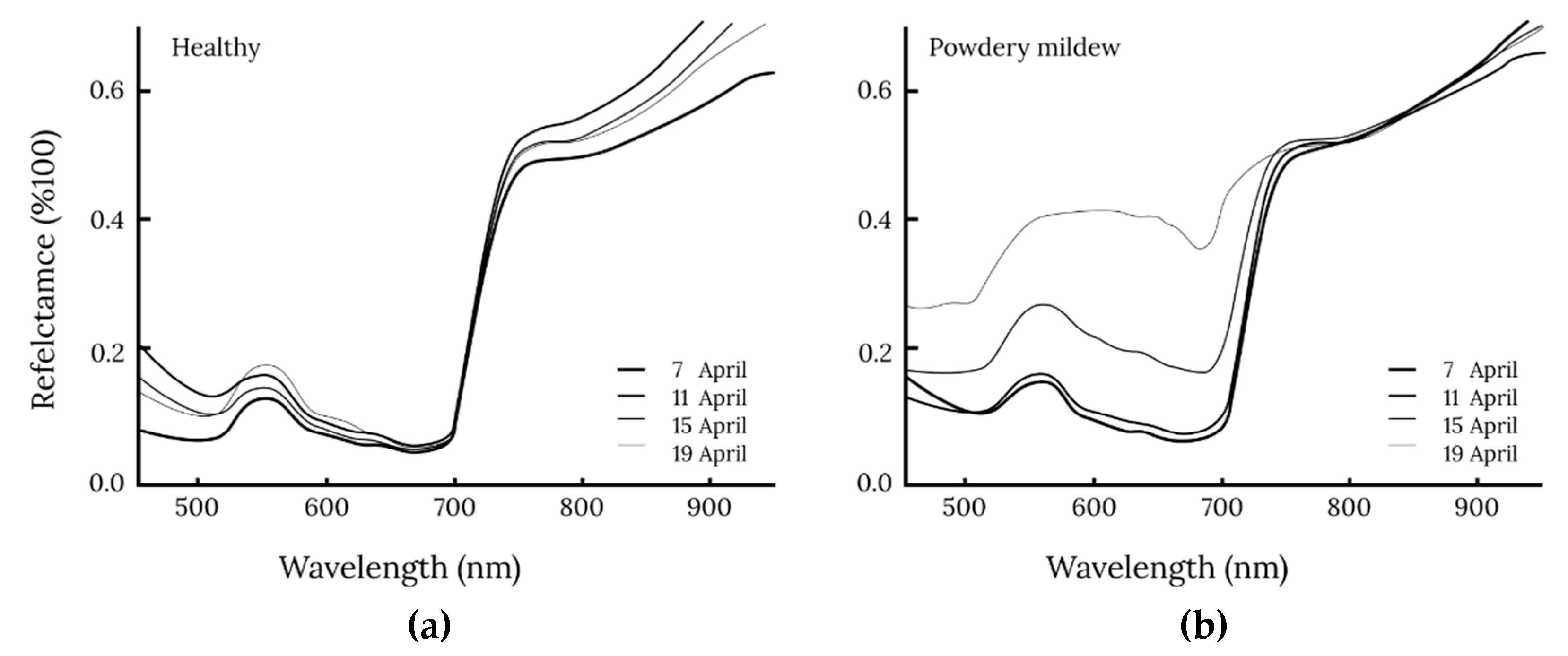
Berdugo et al. (2014) [38] shows the spectral differences between diseased and healthy cucumber leaves in their research on the detection and differentiation of plant diseases among cucumbers (Figure 2). There were only slight differences between diseased and healthy cucumber leaves on the first assessment date. As disease symptoms progressed, differences in visible light became more significant (with a peak of ~650 nm) and at the red edge position at 700 nm.

HSI is an effective tool for agricultural crop monitoring. However, limitations such as changes in the light intensity, background noise, and leaf orientations must be addressed to fully utilize the potential outdoor applications of HSI [39,40]. Reflectance is often the preferred output of the remote sensing data because it is a physically defined object property [41]. However, HSI captures spectral information based on digital number (DN) units [42]. Therefore, an additional process, namely, radiometric calibration, is required to convert DN values to an actual radiation intensity or reflection [43,44]. Radiometrically calibrated images provide long-term and consistent value data [40] that can be effectively used to compute vegetation indices, such as the normalized difference vegetation index (NDVI), and gain an understanding of the status of plants, such as their nitrogen content, chlorophyll content, and green leaf biomass [45].

The primary step in radiometric calibration entails collecting images of Lambertian targets with varying reflectance levels and calculating their average DN to produce radiometric calibration parameters for each band [44,46]. Empirical linear-based approaches can be used when two or more reflectance targets are available on the ground, presuming that the illumination conditions of the targets and the object under study are similar [43,47,48]. Equation (1) represents the basic mathematical formula for calculating the calibrated actual reflectance [43,49].

$$Reflectance=100\times \frac{measurement-dark current}{reference-dark current}$$

(1)

where $measurement$ is the measured image, and $dark current$ and $reference$ are the dark and standard white references. The dark reference can be obtained by covering the lens completely to prevent light from entering the sensor, while the white reference can be obtained by capturing standard white materials with a known reflectance.

2.2. UAV for Agricultural Field Survey

UAVs are drones flown with the assistance of a ground-based flight controller or without an onboard pilot [50]. UAVs can conduct a survey mission to create various map types, including thermal maps, elevation models, and 2D or 3D orthorectified maps that are geographically accurate [51]. A flight mission must be prepared before conducting any UAV survey mission to provide a series of feasible points and optimize image-capturing events [52]. Specialized software programs such as UgCS [53], PIX4Dcapture [54], DroneDeploy [55], or DJI Pilot [56] are typically used in the laboratory to plan the mission (flight and data acquisition) after determining the area of interest, necessary ground sample distance (GSD) or footprint, and inherent parameters of the onboard digital camera. The desired image scale and camera focal length are also calculated to determine the mission flight height [57].

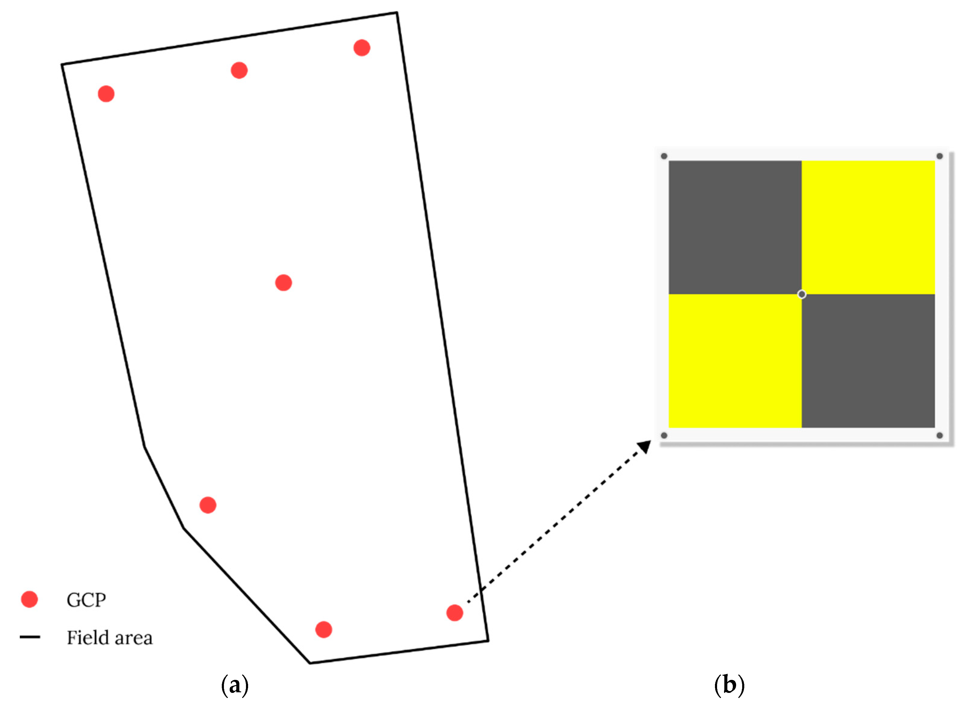
The GSD helps describe the actual size of one pixel on the image, and it is expressed in mm or cm. For example, a GSD of 5 mm implies that 1 pixel on the camera image corresponds to 5 mm on the object [58]. The GSD value depends on the sensor resolution, lens properties, and flight altitude. Figure 3 shows how different flight altitudes affect the GSD. Establishing ground control points (GCPs) in the survey area is another complementary method for accurately mapping the survey area. GCPs are used to determine the exact latitude and longitude of a point on the map on Earth [52]. They should have a clear shape, be visible from a far distance, be easily distinguishable from their surroundings, and have a central location (Figure 4b). GCPs should be included in the captured photographs collected by a UAV to properly align and scale the object of interest for digital reconstruction during postprocessing [58]. According to a previous study [59], using 3 GCPs, 4 GCPs, and up to 40 GCPs to process images resulted in nearly identical accuracy. However, using at least five GCPs is recommended for practical aerial surveys of agricultural fields [60]. It is also important to distribute all GCPs evenly over the study area (Figure 4a).

The imagery collected by UAVs is mainly used to produce 2D maps. The simplest approach to creating a mosaic from aerial imagery is to use photo stitching software such as Image Composite Editor (ICE) [63] to combine several overlapping aerial photographs into a single image. However, it is challenging to precisely estimate distance without geometric correction, which is a procedure that eliminates perspective distortion from aerial photographs. Although simply stitched images are continuous across boundaries, their perspective distortions are not corrected. An orthomosaic is a series of overlapping aerial photographs that have been geometrically corrected (orthorectified) to a uniform scale. This process eliminates perspective distortion from the aerial photographs, resulting in a distortion-free mosaic of 2D images. Geospatial information system (GIS)-compatible maps can be created from orthorectified images for use in cadastral surveying, construction, and other applications [52].

2.3. Deep Learning

Deep learning is a branch of ML that operates based on a neural network principle. It combines low-level features to form abstract high-level features to discover distributed features and attributes of sample data [64]. It automatically extracts and determines which data features can be used as markers to precisely label the sample data [65]. Currently, multilayer perceptions, CNNs, and recurrent neural networks (RNNs) are the three main types of networks [64]. CNNs are commonly used in visual recognition, medical image analysis, image segmentation, natural language processing, and many other applications because they are specifically designed to handle various 2D shapes [66].

As shown in Figure 5, a CNN comprises convolutional layers that serve as feature extractors and fully connected (FC) layers that serve as classifiers at the network’s end [67]. CNNs collect input and process it through convolutional layers with filters (so-called kernels) to detect edges and boundaries. They also collect other features to identify objects in images. Each filter generates a feature map that travels through the network from one layer to the next [68]. Once the features are extracted, they are mapped by a subset of FC layers to the final outputs of the network to generate probabilities for each class [69]. The final output of CNNs is a probability or confidence that indicates the class that each input belongs to [67]. CNN tasks can be divided into image classification, object detection, and image segmentation, depending on how the prediction is made (Figure 6).

Image classification is the process of organizing images into a predefined category or class [70]. However, it is challenging when there are multiple classes or objects in a single image. Object detection is the subsequent stage of CNN development and aims to classify and localize each object in an image within a bounding box [68]. This method requires additional steps to preclassify the image into regions or grids [71] and subsequently classify the object category or class for each bounding box to pinpoint the location of an object. Each box also has a confidence score that indicates how often the model believes this box contains an item [68]. However, it is more challenging to separate and categorize all the pixels related to the object. This operation is called object segmentation. Object segmentation is a pixel-level description of an image. It forms a boundary according to the shape of the corresponding object rather than creating bounding boxes that separate each object. It provides meaning to each pixel category and is suitable for understanding demanding scenes, such as the segmentation of roads and non-roads in autopilot systems, geographic information systems, medical image analyses, etc. [72,73].

Since a significant amount of data is required to achieve a high-performing deep-learning-based model, the model performance is expected to improve as the data volume increases [67]. The model must also generalize the data, which means that it must learn from both the training data and the unseen data [74]. Large training datasets are often essential to ensure generalizability. Relatively small datasets (hundreds of cases) may be sufficient for specific target applications or populations. Large sample sizes are necessary for populations with significant heterogeneity or when there are small differences between imaging phenotypes [75,76].

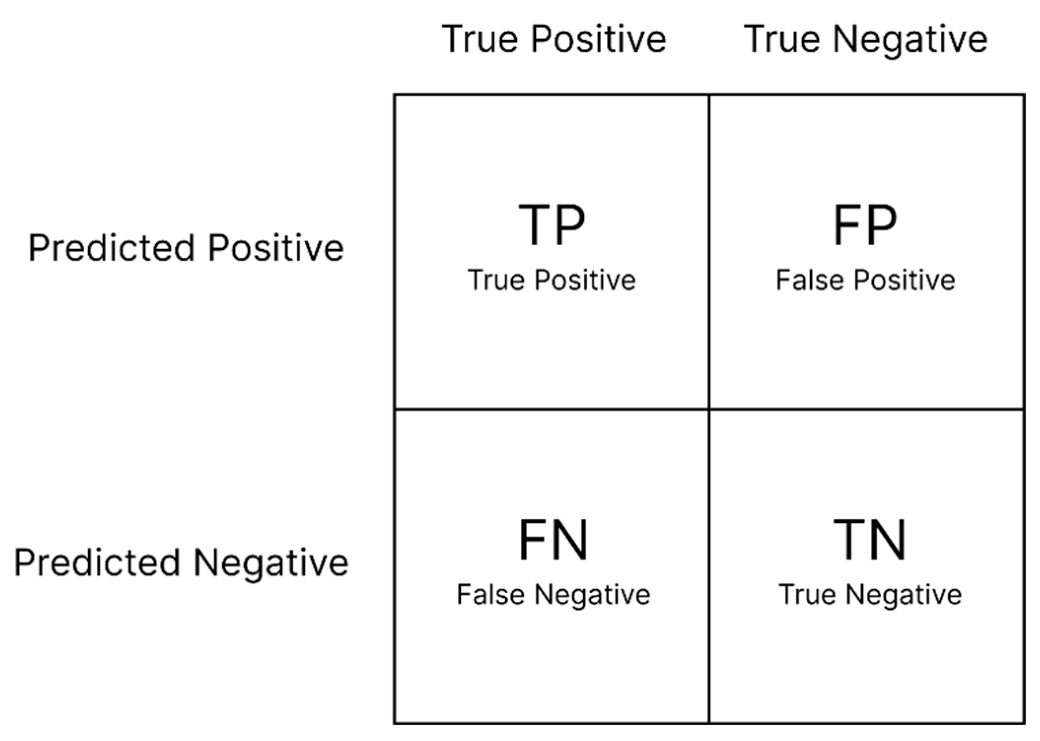
Evaluating deep learning models is an essential part of any project. A confusion matrix is widely used to measure the performance of classification models, and it displays counts from predicted and actual values (Figure 7). True negative ($TN$) represents the number of accurately classified negative examples, true positive ($TP$) indicates the number of accurately classified positive examples, false positive ($FP$) represents the number of negative samples classified as positive, and false negative ($FN$) represents the number of positive samples classified as negative [77]. Additional evaluation matrices can be created to assess the model’s accuracy ($ACC$), precision ($P$), sensitivity ($Sn$), specificity ($Sp$), and F-score. These performance metrics can be calculated using Equations (2)–(6) [78,79]:

$$ACC=\frac{TP+TN}{TP+TN+FP+FN},$$

(2)

$$P=\frac{TP}{TP+FP},$$

(3)

$$Sn=\frac{TP}{TP+FN},$$

(4)

$$Sp=\frac{TN}{TN+FP},$$

(5)

$$Sp=\frac{TN}{TN+FP}.$$

(6)

Intersection over union (IOU) is commonly used to evaluate object detection or image segmentation models (Equations (7)). It divides the overlapping area between the predicted bounding box and the ground-truth bounding box by the union area between them.

$$J\left(B_p, B_{gt}\right)=IOU=\frac{area \left(B_p{\displaystyle \cap } B_{gt}\right)}{area \left(B_p{\displaystyle \cup } B_{gt}\right)}$$

(7)

where $B_p$ and $B_{gt}$ represent the prediction box and ground-truth box, respectively. The IOU is calculated by dividing the overlapping area by the union area between $B_p$ and $B_{gt}$. Model prediction can be evaluated by comparing the IOU with a specific threshold. The prediction is correct if the IOU is greater than the threshold and incorrect if the IOU is lower than the threshold [80].

3. Related Works

HRS has been widely used for various applications in numerous study fields. Four keywords were used to uncover publications for this review: UAV, hyperspectral, plant disease, and deep learning. This review focuses on the target disease, system operation, workflow, deep learning algorithm, and results.

Yu et al. (2021) [81] investigated early pine wilt disease (PWD) discovered in the Dongzhou District of Fushun City, Liaoning Province, China. A ground survey was conducted to identify PWD symptoms based on the morphology and molecular analysis of tree samples to confirm the presence of the disease. The location of the tree samples was recorded as ground-truth data using a hand-held differential global positioning system (DGPS). The samples were classified based on the early, middle, and late infection stages.

Data acquisition was conducted using DJI Matrice 600 equipped with a Pika L hyperspectral camera and an LR1601-IRIS LiDAR system. The flight had a 120 m height, a 60% overlap, and a 3 m/s flight speed. Radiometric calibration was performed based on a tarp for reflectance correction, and six GCPs were used for geometric correction.

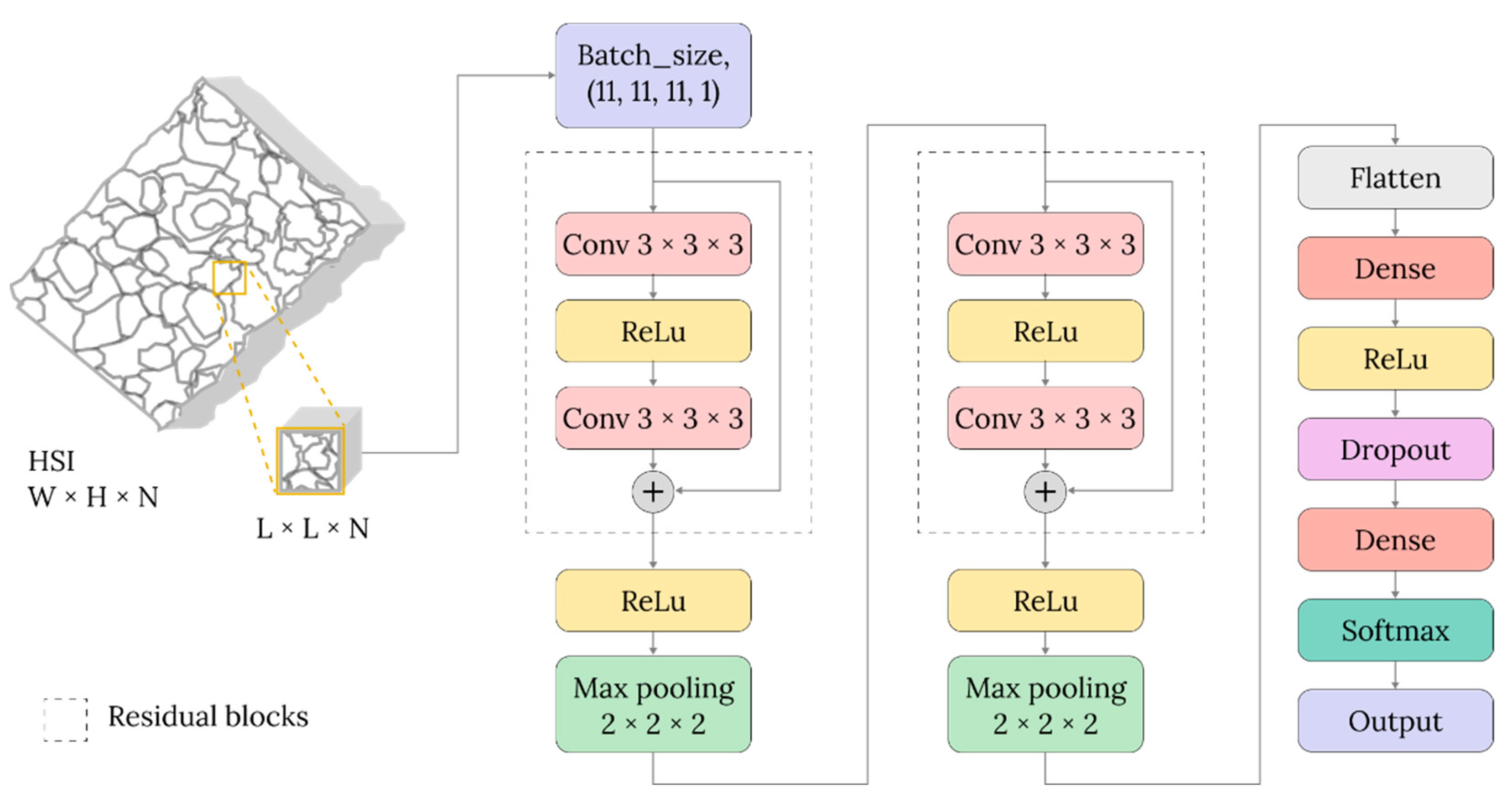
This research proposed a 3D-Res CNN model based on pixel-level features, and the input data were a set of spatial–spectral neighboring cubes around the pixels. Image blocks were extracted from the hyperspectral cube using a 3 × 3 × 3 kernel and an 11 × 11 window. Additionally, 11 wavelengths were extracted using the principal component analysis (PCA) method to make the model more rapid and lightweight. The 3D-Res CNN model consists of four convolution layers, two pooling layers, and two residual blocks. The 3D convolution operation can be used to retain both spatial and spectral data.

The 3D-CNN, 2D-CNN, and 2D-Res CNN models were compared to evaluate the performance of the 3D-Res CNN model in identifying PWD-infected pine trees based on hyperspectral data. The 3D-Res CNN model outperformed the other models, with an overall accuracy (OA) of 88.11% and an accuracy of 72.86% for identifying early infected pine trees. A residual CNN block, which was used in the model, solved the vanishing gradient problem and improved the classification accuracy.

Zhang et al. (2019) [82] investigated winter wheat infected by yellow rust disease in the Scientist Research and Experiment Station of China Academy of Agricultural Science in Langfang, Hebei Province, China. Four experiment plots were prepared for data collection: two plots were infected with yellow rust wheat, and two plots were left uninfected. A DJI S1000 UAV system equipped with a UHD 185 firefly (Cubert) snapshot-type hyperspectral camera was used as the data acquisition system. The images were mosaicked, and then, 15,000 cubes with a size of 64 × 64 × 125 were cropped and extracted to build the deep learning model. Data augmentation was performed through a small random transformation with a rotation, flip, and mirror to prevent the model from overfitting.

The proposed deep learning model consists of several Inception and ResNet blocks, an average pooling layer, and an FC layer, and it classifies samples into three categories: rust, healthy, and others. The ResNet block was used to build a feasibly thin deep learning model while maintaining or enhancing its performance. He et al. (2016) [83] demonstrated that residual learning can overcome the vanishing/exploding gradients in deep networks. Since the performance of the model is also influenced by the width and kernel size of the filter, an Inception–ResNet structure [84] was used to address this problem by employing different kernel sizes.

The proposed model was compared to a random forest (RF) ML model to evaluate its performance. The Inception–ResNet CNN model achieved a higher accuracy (85%) than the RF model (77%). The proposed model was able to perform better because it could account for both the spectral and spatial information to detect the disease, compared to the RF, which only accounts for the spectral information. Relying on spectral information alone was not feasible because the spectral information from each class had a high variance.

Shi et al. (2022) [85] investigated potatoes infected by late blight disease. The experiment was conducted in Guyuan county, Hebei province, China. DJI S1000 equipped with a UHD-185 (Cubert) hyperspectral camera was used as the data acquisition system. Four types (classes) of ground-truth data were investigated: healthy potatoes, late blight disease, soil, and background (i.e., the roof, road, and other facilities). The hyperspectral data were acquired at a 30 m flight height.

The research proposed a deep learning model called CropdocNet, which consists of multiple capsule layers, to model the effective hierarchical structure of spectral and spatial features that describe the target classes. The model employed a sliding window algorithm with 13 × 13 patch sizes and was trained with 3200 cubes. The proposed model showed significant differences when compared to conventional ML algorithms, support vector machine (SVM), RF, and 3D-CNN, achieving a maximum accuracy of 98.08%.

4. General Workflow for Hyperspectral-Based Plant Disease Detection

UAV-borne HRS is considered a new field of study that is continuously evolving. New instruments and methods are being developed to obtain improved results. Three papers that matched the keywords UAV, hyperspectral, plant disease, and deep learning are reviewed in this paper. Several challenges must be overcome when conducting UAV-borne HRS research for disease detection. First, it is a multidisciplinary field of study that involves researchers from multiple disciplines; therefore, each party must collaborate effectively. Second, a huge amount of data is required to train the deep learning model. The experiment cannot produce a massive number of diseases as training data. Since disease occurrence in the actual field is usually low, there is a limited number of available datasets to train the deep learning model. However, some generalizations can be made regarding the research workflow based on the matched research keywords and other related research.

4.1. Field Preparation

The first research step for developing a deep learning model for disease detection is to establish an experiment site. The site must have a sufficient number of healthy and diseased samples. Two types of methods are usually used when establishing or choosing a site. In some studies, separate experiment plots were created, and the disease was inoculated in one or more plots to create healthy and diseased samples [82,85,86]. For example, Guo et al. (2021) [87] conducted research on wheat yellow rust detection. Three plots were set up (two inoculated plots and one healthy plot), each with an area of 220 m². Wheat yellow rust fungus spore suspensions were prepared and sprayed on the wheat leaves with a handheld sprayer. Meanwhile, pesticides were sprayed on the healthy plot to prevent it from being infected by the yellow rust. However, disease inoculation is only suitable for small sample sizes and cannot be used in actual large-scale applications [81], and the success rate is also not guaranteed. Additionally, since different diseases (e.g., PWD disease) are initially transmitted by insects via different transmission modes, artificial disease inoculation could cause various symptoms [88]. Therefore, other researchers chose experiment sites where plants or trees are naturally infected by the disease [81,86,89,90].

4.2. Ground Survey

Another crucial stage is to conduct a ground survey after the experimental site has been established. The diseased plant on the acquired images must be validated and matched with the diseased plant on the actual site [81,85]. The exact position of the diseased plant at the experiment site must also be identified in the acquired images. The different visual features of the samples displayed in the images can be used to differentiate each class. Another viable option is to mark the sample’s position based on its GPS location [91]. The infection stages can be determined by identifying the sample morphology. For example, Yu et al. (2021) [92] conducted research to detect PWD disease infection. A ground survey was conducted to determine the infected plants and build a ground-truth dataset. The PWD infection was divided into several stages by considering resin secretion, growth vigor, and the color of the needles. Afterward, the disease infection can be further validated by performing sample molecular identification using polymerase chain reaction (PCR) analysis [93].

Disease severity refers to how a particular disease spreads throughout a plant and affects its growth and yield. It is most often expressed as a percentage or proportion. Most studies have defined disease severity as the area of disease lesions or symptoms with respect to the area of the leaf. Therefore, researchers have used deep learning-based image classification to solve the problem based on the area of leaves covered by lesions [94].

4.3. Data Acquisition

Data acquisition involves UAV-based hyperspectral system configuration and flight planning. UAV platforms must be able to carry payloads safely and stably because most hyperspectral camera systems require a microcomputer for operation. Figure 8 presents examples of a typical UAV-based hyperspectral camera system configuration.

The GSD, or ground resolution, must be defined before conducting data acquisition. Ground resolution is typically acquired by deriving the camera properties (such as sensor resolution, focal lengths, or FOV), and it depends on the samples and application. Most hyperspectral cameras have lower resolutions than digital RGB cameras. Therefore, the ground resolution must be calculated carefully to obtain good results.

In forestry, flights are conducted at heights between 70 m [88], 100 m [95], and 120 m [81,96] above the ground for disease detection, with a ground resolution of 0.4–0.56 m. However, agricultural field applications tend to have a smaller sample size (plant) and flat ground. Flying between 20 m [97] and 30 m [82,85,87,98,99,100] above the ground allows for the collection of more detailed field information with 1 to 3.5 cm of ground cover.

Weather factors should be considered during data acquisition. The flight should be conducted on a sunny day to achieve a good DN value and uniform illumination all over the experiment site [101]. Flying on a windless day should also be considered to reduce UAV vibration caused by the blowing wind. This is because the wind could move the plants, causing them to have different positions in each photo captured and resulting in blurry images [102].

4.4. Image Preprocessing

Aerial images captured from UAVs must be processed to reduce errors and obtain high-quality hyperspectral images for plant disease analysis. This process is called preprocessing, and it includes image mosaicking, geo-referencing, radiometric calibration, and in some cases, dividing the images into small patches as input for the model. Mosaicking is the process of combining overlapping field images into one single image. It is important to use an orthomosaic image because this type of image corrects perspective distortion and provides true distance measurement. Agisoft Metashape [103], PIX4Dmapper [104], or DJI Terra [105] are commonly used, reliable software programs for creating orthomosaic images. Geo-referencing is the technique of assigning each pixel in an image to a specific location in the real world. Georeferencing is performed by utilizing GCPs on the field. This process can provide accurate geoinformation about an image and rectify its overall shape to resemble how it looks in the real world. Georeferencing can be conducted in software such as ArcGIS [106], Agisoft Metashape [103], PIX4Dmapper [104], or ENVI [107]. The following step is radiometric calibration. The raw data captured by the hyperspectral camera are simply arbitrary numbers known as a digital number (DN), which must be converted into radiation. Because the field observations may occur on different days and because slight differences in light intensity between flights are unavoidable, converting the radiation value to reflectance is required to provide a consistent value. This is accomplished by calibrating the radiation value to a known reflectance, which in this case, is a reflectance tarp set in the field during data collection.

4.5. Feature Extraction

Disease detection begins with feature extraction. The disease might be indicated by different colors. In the case of hyperspectral images, further differences can be found beyond visible light bands. Furthermore, a classifier model can be built to detect diseased areas by using spectral data as input variables. Having a distinct spectral signature, the model can distinguish between healthy and diseased samples. However, using only spectral data as variables may not be entirely robust. Different environmental conditions, such as sunlight and shades, can affect the spectral data of the samples for outdoor applications. The model classification accuracy can be increased by considering the shape caused by the disease or by employing the spatial feature of the data. Feature extraction aims to extract and form new feature vectors for plant disease detection by combining and optimizing the spectral, spatial, and texture features and then delivering them to a set of classifiers or ML algorithms [36].

4.5.1. Spectral Features Extraction

• Using full spectrum

Having numerous spectral data points is one of the advantages of using a hyperspectral camera. Different intensities of particular spectral bands within the hyperspectral data can be used to identify disease symptoms. Full spectrum can be used when short-range dependencies between spectral wavelengths must be preserved [1]. A classifier model can be built based on these differences by assigning each band as a variable, and classifications can be made by classifying one pixel at a time.

2.

Band reduction methods

Hyperspectral images have stacks of wavelength bands that are treated as variables for the model. In most cases, adjacent wavelengths have high similarity, which causes a large amount of data redundancy, which has a negative effect on classification performance [108]. Therefore, selecting the characteristic bands or variables that can fully represent all wavelength information is important. Dimensionality reduction methods, such as PCA, minimum noise fraction (MNF) algorithm, linear discriminant analysis (LDA), stepwise discriminant analysis (SDA), partial least squares discriminant analysis (PLS-DA), and successive projection algorithm (SPA), can be used to decrease collinearity between variables and increase model performance [36].

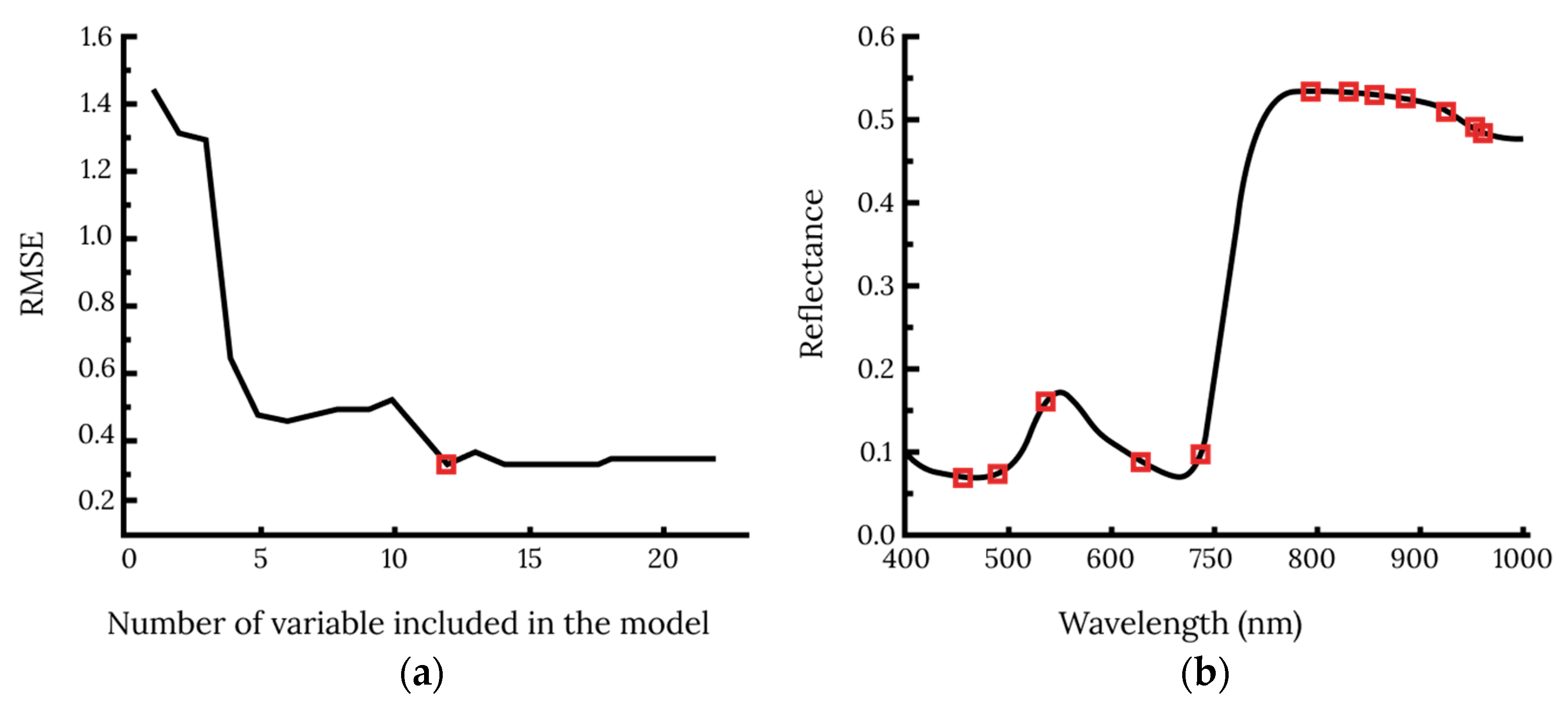
PCA is one of the most common feature selection methods, and it transforms the original data linearly. This method processes the original data and generates features known as components. The components are statistically uncorrelated and keep the maximum amount of information [108]. Contrary to using the original spectral data as the model input, using the PCA components results in a low number of variables while maintaining adequate information. Additionally, SPA is a variable selection technique that can minimize the influence of collinearity between spectral variables and extract useful information from the spectral data [109]. Xuan et al. (2022) [12] attempted to detect early wheat powdery mildew disease using HSI. They used SPA to filter out the effective wavelengths from the whole spectrum. Twelve effective wavelengths were obtained when the RMSE reached the minimum value of 0.31, and the wavelength selection processes are shown in Figure 9.

Dimensionality reduction techniques are used to reduce the number of variables used as model input while retaining as much information as possible in those reduced variables. The amount of collinearity within the spectrum is minimized, and the reduced variable can be used to represent the whole spectrum data. These techniques condense redundant information across the whole spectrum, thereby improving classification performance and reducing computational costs.

3.

Vegetation indices

A Vegetation Index (VI) is a value computed by transforming the observations of two or more spectral bands designed to emphasize the spectral properties of green plants, allowing them to be distinguished from other image components [110]. Spectral features can be extracted from hyperspectral data by analyzing and comparing vegetation indices between diseased and healthy crop samples and using them as variables. Vegetation indices numerically represent the relationship between the different wavelengths reflected by plant surfaces. Vegetation indices represent the physiological and morphological characteristics of a plant, such as its water content, biochemical composition, nutrient status, biomass content, and diseased tissues [111].

Marin et al. (2021) [112] extracted 63 vegetation indices from multispectral images to detect coffee leaf rust disease using several ML models. In their research, Modified Normalized Difference Red Edge (MNDRE) has the highest contribution to the model. Similarly, Abdulridha et al. (2019) [99] studied 31 vegetation indices to develop a radial basis function (RBF) and KNN for citrus cancer disease detection. It was found that the Water Index (WI) was the most influential band in distinguishing healthy and diseased leaves. Additionally, Anthocyanin Reflectance Index (ARI) and Transform Chlorophyll Absorption in Reflectance Index (TCARI 1) can accurately differentiate healthy citrus trees from cancer-infected citrus trees. Zhao et al. (2020) [113] used six typical vegetation indices related to biomass, photosynthetically active radiation (PAR), leaf area index (LAI), and chlorophyll contents to estimate cotton crop disease. Some of these vegetation indices include the NDVI, green NDVI, Enhanced Vegetation Index, and Soil-Adjusted Vegetation Index (

Table 1. List of commonly used vegetation indices related to plant health [110].

Vegetation Indices	Formulas	Applications
Normalized Difference Vegetation Index	NDVI = $\frac{(R_{800}-R_{670})}{(R_{800}+R_{670})}$	NDVI assesses plant health by dividing the difference in the intensity of reflected light in the red and infrared regions by the sum of these intensities.
Green Normalized Difference Vegetation Index	GNDVI = $\frac{(R_{800}-R_{550})}{(R_{800}+R_{550})}$	GNDVI is calculated by dividing the difference between infrared and green light reflectance; it is sensitive to chlorophyll concentration.
Ratio Vegetation Index	RVI = $\frac{R_{800} }{R_{670}}$	RVI is the ratio between the near infrared and red band reflectance.
Enhanced Vegetation Index	EVI = $\frac{2.5(R_{800}-R_{670})}{(R_{800}+6R_{670}-7.5R_{450}+1)}$	EVI is related with biomass; leaf area index (LAI).
Normalized Difference Red-Edge	NDRE = $\frac{(R_{800}-R_{720})}{(R_{800}+R_{720})}$	NDRE is used to measure chlorophyl amount in the plants; it provides more accurate result for middle and late season crops.
Soil-Adjusted Vegetation Index	SAVI = $\frac{\left(1.5\right)(R_{800}-R_{670})}{(R_{800}+R_{670}+0.5)}$	SAVI is best suited in areas having low vegetation cover
Leaf Chlorophyll Index	LCI = $\frac{(R_{850}-R_{710})}{(R_{850}+R_{680})}$	LCI is used to measure chlorophyll content
Modified Chlorophyll Absorption Ratio Index	MCARI = $(R_{700}-R_{670})-0.2 (R_{700}-R_{550})*(R_{700}/ R_{670})$	MCARI indicates the relative abundance of chlorophyll.

). It was found that Enhanced Vegetation Index (EVI) is the most suitable for detecting cotton diseases. A comprehensive list of vegetation indices can be found in the Index-Data-Base (IDB) [114].

The NDVI is a common vegetation index used for crop health monitoring. However, it is not suitable for identifying the causal agent of crop diseases. The NDVI does not follow specific wavebands that represent physiological changes caused by pathogens. In general, VIs are a simple and effective algorithm that can be used for plant condition assessment. Disease identification can be accomplished using VIs by evaluating leaf senescence, chlorophyll content, water stress, etc. However, VIs are not disease specific because they are only related to plant biophysical properties. The majority of the VIs are quite specific and only performed well with the datasets for which they were designed [110]. Spectral Disease Indices (SDIs) are a more accurate representation of disease-infected plants, and it is a ratio of the different disease spectral bands extracted based on spectral responses from the diseased vegetation. SDIs are specific and unique to each vegetation, disease, and infection stage because the disease may uniquely affect the leaf reflectance spectrum [115]. Disease indices can be formulated for specific diseases, or an existing SDI can be used. Mahlein et al. (2013) [116] developed spectral indices to detect Cercospora leaf spot, rust, and powdery mildew disease in sugar beet plants. Meng et al. (2020) [117] developed a disease index to detect corn rust and classify its severity. SDIs have the potential to discriminate and differentiate one plant disease from another because they are sensitive to a particular disease.

4.5.2. Spatial Features Extraction

Spatial features are numerical representations of an image in a single band based on a descriptor. Shape, size, orientation, and texture are examples of spatial characteristics. Tetila et al. (2017) [118] employs a machine-learning method for automatic soybean leaf disease detection. Spatial features include texture (repetitive patterns that present in an image associated with roughness, coarseness, and regularity), shape (describes images according to the contour of objects), and gradient (represents derivatives in different directions of the image). Hlaing and Zaw (2018) [119] used the Scale Invariant Feature Transform (SIFT) to find texture information classified as tomato plant disease using a combination of texture and color features. They used the Scale Invariant Feature Transform (SIFT) to find the texture information, containing details about the shape, location, and scale. Because a machine learning model can only accept numerical inputs, hyperspectral images must be converted or transformed into a numerical value that represents their spatial features.

Vegetation Index generation, SDI generation, and dimensional reduction methods are feasible methods for creating features used for developing ML models. Multiple steps and complex processes are involved in feature extraction. Engineering or extracting features from raw data is a challenging task, and sometimes, the solutions are specific to each case or dataset. However, this process can be eliminated in CNN models because the essential features are located during the dataset training [111].

4.6. Disease Detection Approaches

Mosaicked aerial images are large-sized images that contain a huge amount of information regarding the entire field. They must be divided into smaller patches or segments in order to perform effective disease classification. The divided images can then be transferred to a classifier to determine the presence of the disease and subsequently combined as a whole image with the delineated diseased area. Aerial images are divided differently, depending on the research object, and they can be optimized with a classifier to obtain maximum performance. Several studies have divided the images into 11 × 11 [81], 13 × 13 [85], 32 × 32 [86], 64 × 64 [82,120], 128 × 128 [90], 224 × 224 [121], 256 × 256 [90], and 800 × 800 [88] patches using various approaches, including a segmentation process [89,122,123], to create the dataset.

The following are numerous methods used for effectively processing aerial images for disease detection:

• Patches or sliding windows and CNNs [82,120,124]: These methods are the most straightforward methods for detecting and localizing plant disease. They entail dividing the original images into smaller square images (patches) and using them as CNN input. After each patch or window is classified, the end result can be achieved by recombining them into a whole image. However, most of the time, these methods are not suitable for real-time usage because they tend to be computationally expensive.
• Segmentation and CNN or ML [89,90,122,123]: This method has a similar operation to the sliding window algorithm; however, the image is segmented or separated into regions using different segmentation algorithms rather than divided into smaller square patches. The segmented regions have arbitrary shapes that contain similar features within each segment. For plant disease detection, the segments can be designed to follow the shape of each leaf or some region of the leaf that has similarities. The classification is performed by extracting the segments and transferring them to a classifier model (CNN or ML). After recombining each classified segment, the result would look like the diseased leaves are delineated. This method identifies diseased plants with high accuracy.
• Object detection [88,93,125,126,127]: This method utilizes CNN-based object detection algorithms, such as YOLO, Fast R-CNN, and Faster R-CNN. The input image for this method is between 244 and 1000 pixels. This method can generate bounding boxes that surround the object, detect the disease, and find its location in the image. This method can be used in real time because it has a faster prediction speed. This is because this method simultaneously detects multiple objects in a single image rather than dividing the image into smaller patches like the previous two methods. However, there is currently no information about its accuracy for detecting disease based on hyperspectral images (further research is needed).
• Image segmentation algorithm: This method has been used to detect plant diseases or weeds in various studies [86,90,91,128,129,130,131]. It classifies each pixel in the image into corresponding classes. This method is similar to object detection, but it generates an arbitrary region shape that matches the shape caused by the disease rather than generating bounding boxes around the disease area. The segmentation method aims to provide a fine description of these regions by delimiting the boundary of each different region in the image [132].
• Pixel-based CNNs [81,85]: This method has the same principle as the sliding window method. However, the input data are a set of spatial–spectral neighboring cubes around pixels rather than the whole image (Figure 10). The patch size of the input information from the acquired image is smaller than that of the image-level classification task. Generally, convolution kernels with small spaces can be used to prevent excessive input data loss [81]. The resulting output is a map of regions with an arbitrary shape, and it classifies the diseased area.
• Heat map and conditional random field (CRF) [121]: This method uses CNNs as a heatmap, which is then reshaped to accurately segment the lesions using CRF.

All the abovementioned techniques can classify and locate diseases within the acquired aerial images. Patches or sliding windows combined with CNNs and object detection produce bounding boxes around the diseased area, while the other techniques produce segments or regions with a similar shape to the diseased area. Object detection only allows for the creation of rectangular bounding boxes, resulting in the localization of the extra areas with no disease lesions and symptoms. The segmentation method produces the most accurate results when used to calculate the infected leaf regions with respect to the entire leaf [94].

Table 2. Summary of the different methods for disease detection.

Plant	Disease	UAV System	Data	Model	Algorithm	Input Features	Evaluation	Ref
Pine	Pine wilt disease	DJI M600, LR1601 IRIS LIDAR, Pika L HSI	Hyperspectral	3D-Res CNN	Sliding window	11 × 11 × 11 hyperspectral block	88.1 acc	[81]
Wheat	Yellow rust	DJI S1000, UHD 185 Cubert	Hyperspectral	Inception-Resnet	Sliding window	64 × 64 × 125 hyperspectral block	85 acc	[82]
Potato	Blight	DJI S1000, UHD-185 Cubert	Hyperspectral	CropdepcNet	Sliding window	13 × 13 × 125 hyperspectral block	95.75 acc	[85]
Pine	Rotting, powdery mildew, and wood nematode	DJI Phantom 4Pro, FC6310	RGB	Inception V3 + AdaBoost	Region classification	64 × 64 × 3 RGB patch	0.957 recall	[120]
Radish	Fusarium wilt	DJI Phantom 4	RGB	VGG-A	Region classification	200 × 200 × 3, KNN ROI	93.3% acc	[89]
Pine	Nematode disease	FeimaD200, RedEdge-MX	Multi spectral	SCANet	Image segmentation	128 × 128 × 5	79.33% acc	[90]
Corn	NLB	DJI Matrice 300 RTK, P1	RGB	DenseNet169	Sliding window	1000 × 1000 × 3	100% acc	[122]
Soybean	Asian rust, target spot, mildew, pwdery mildew	Phantom 3 Pro, Sony EXMOR	RGB	Inception-v3 FT 75%, Resnet-50 FT 50%, VGG-19 FT 100%, Xception FT 100%	Region classification	256 × 256 × 3, SLIC Segmentation	99.04%, 99.02%, 99.02%, 98.56%	[123]
Pine	PWD	DJI Phantim 4 Multispectral	Multispectral	Faster R-CNN, YOLOv4	Object detection	800 × 800 × 6	60.98% map, 57.07% map	[88]
Pine	PWD	DJI Phantom 4 RTK, CMOS	RGB	YOLOv3 Darknet53, YOLOv4 MobileNet, R-CNN ResNet50m Faster R-CNN ResNet101	Object detection	1024 × 1024 × 3	64% map, 63.2% map, 60.2% map, 62.2% map	[93]
Grape	Flavescence Doree	DJI Matrice 210 v2, Zenmuse XT2	RGB	Faster R-CNN ResNet 101	Object detection	1024 × 1024 × 3	82% map	[125]
Pine	PWD	CMOS Sony Rx R12	RGB	FPN + ResNet101	Object detection	800 × 800 × 3	89.44% map	[126]
Vine	Mildew	Quadcopter drone Scanopy, MAPIR Survey2	Multispectral	SegNet	Image segmentation	360 × 480	90.23% acc	[86]
Wheat	Yellow rust	DJI Sentinel 2	RGB	PSPNet	Image segmentation	256 × 256 × 3	98% acc	[128]

provides a summary of the different methods for disease detection.

4.7. Model Evaluation

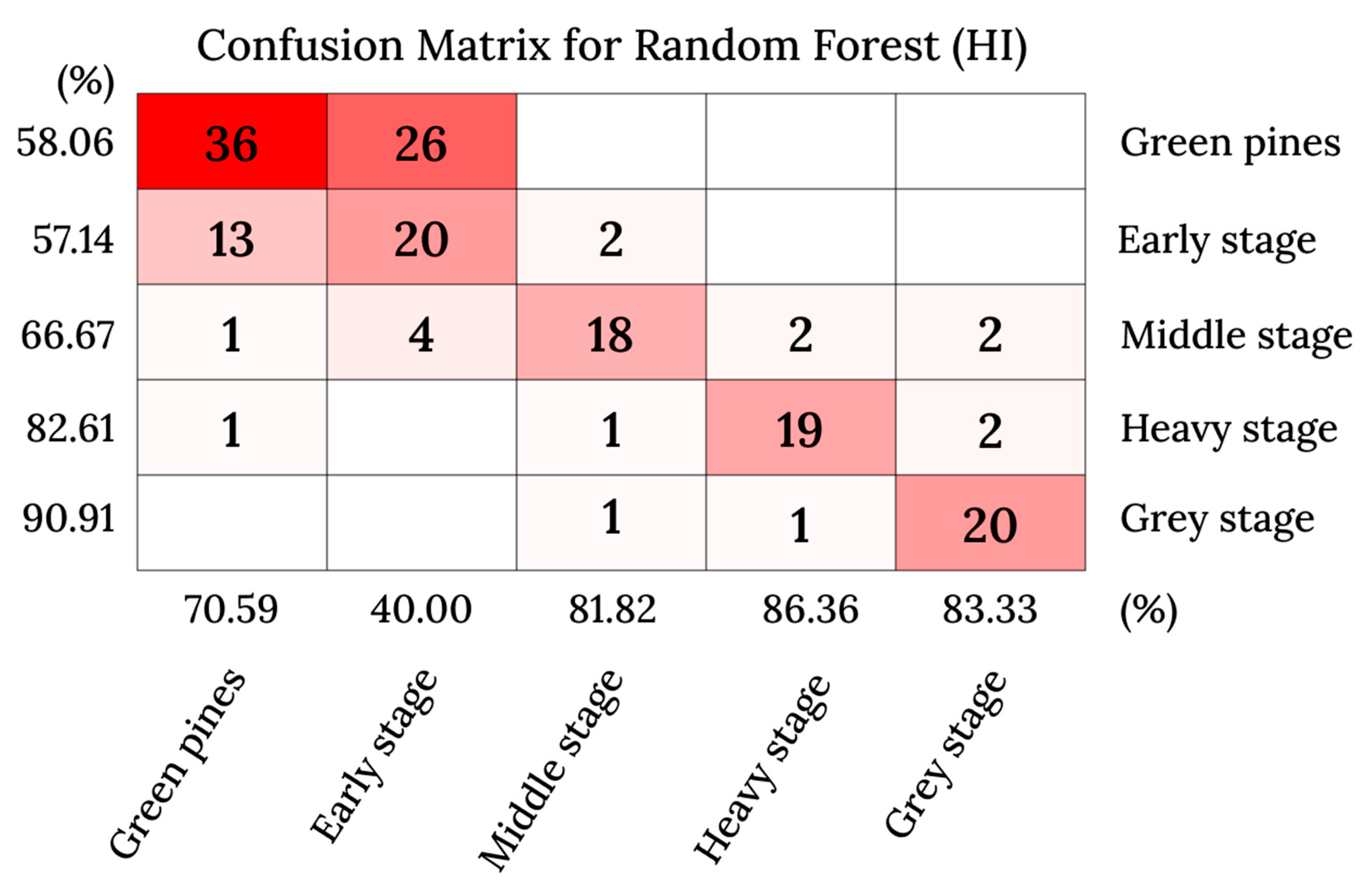
Model evaluation is the process of assessing the performance of a model, and it can be performed using evaluation matrices. A confusion matrix is one of the evaluation matrix methods that allow for a model evaluation by visualization, and it can be used for single or multiclass classification. It compares the OA of the model and the accuracy within each class (Figure 11). It reveals the categories that the model excels at and those that it struggles with. Researchers can rely on this information to further enhance the performance of a model or evaluate the dataset for a specific class.

In some cases, accuracy may not be very reliable in describing model performance. Wu et al. (2018) [133] developed a deep learning model to detect corns infected by northern leaf blight. They discovered that even though the accuracy was 97.76%, the model prediction produced many false positives and negatives, indicating that the training set did not accurately represent the empirical distribution. The false positive and negative predictions were reduced by including many more negative samples, and the model was able to delineate the disease more accurately.

4.8. The Importance of Spatial Resolution

4.8.1. Sub-Pixel Problem and Spectral Unmixing

Aerial hyperspectral imagery, unlike lab tests, captures images from above. The importance of choosing an appropriate flight height is highlighted here; a lower altitude is better, but field coverage will be reduced due to the flight time. Pixel sizes for aerial remote sensing, particularly for hyperspectral images, range from centimeters to meters, implying that the pixels will typically contain information from more than one material [2]. Materials of interest (target) may not be resolved in a single pixel [134].

Mahlein et al. (2012) [135] found that a spatial resolution of 0.2 millimeters per pixel was optimal for visualizing disease symptoms in their research for small-scale analysis of sugar beet disease. A sensor system’s spatial resolution is critical for detecting and identifying leaf diseases. Characteristic symptoms were no longer detectable at spatial resolutions of 3.1 and 17.1 mm; the spectral signal contained both healthy and diseased tissue. The number of pixels with mixed information increased as spatial resolution decreased, while reflectance differences decreased.

Kumar et al. (2012) [136] investigated citrus green disease known as Huanglongbing (HLB) using aerial hyperspectral imagery with a spatial resolution of 0.7 m. More pixels were discovered using linear spectral unmixing techniques, indicating HLB (HLB-infected pixel) infection. The detection of HLB-infected pixels after spectral unmixing resulted in more match to the ground-truth data. Using a spectral unmixing algorithm may enable hyperspectral imaging to detect smaller and potentially earlier diseases.

4.8.2. Comparison with RGB Camera

UAV-based hyperspectral camera systems require a detailed setup in order to operate, and they tend to be more expensive than RGB cameras. Moreover, hyperspectral cameras tend to have a lower spatial resolution in exchange for high spectral resolution. In the studies discussed in this review, the observed plant disease was indicated by morphological changes, which can be identified based on visible wavelengths. Considering the cost-effective value of an RGB camera and its high resolution [82], comparative studies on the performance of RGB and hyperspectral cameras on the same samples should be one of the further areas of interest.

Ahmad et al. (2022) [122] conducted a study on detecting crop diseases using DenseNet169-based RGB cameras. The disease was apparent on the leaf surface, and the used model could achieve the best results with the lowest loss value of 0.0003 and testing accuracies of up to 100%. It can be concluded that RGB imagery has great potential to be used for identifying diseased regions.

Wu et al. (2021) [93] studied PWN-infected pine trees. They discovered noticeable spectral differences between the healthy and diseased pine trees at 638–744 nm wavelengths. They also discovered that the healthy pines (HPs), late-stage infected pines (AIs), and early-stage infected pines (PIs) had different gray values in the RGB images. They concluded that RGB images are sufficient for distinguishing PIs and HPs.

4.9. Limited Dataset Handling

The accuracy of a CNN model may not be satisfactory without sufficient training samples. However, gathering sufficient training samples for large-scale applications can be challenging. Some plant diseases have a low incidence, and the cost of acquiring disease images is high, resulting in only a few or dozens of disease images being collected [137]. For example, gathering diseased tree samples in actual forestry management requires a considerable workforce and a significant amount of material resources [91]. Therefore, it is crucial to ensure that the model is accurate even with few training samples.

However, a limited dataset can be handled by designing a reasonable network structure to reduce the sample requirements. Liu et al. (2020) [73] developed a more accurate CNN method for diagnosing diseases that affect grape leaves. A depth-separable convolution rather than a conventional convolution was used in the model to prevent overfitting and to minimize the number of parameters. The initial structure was applied to the model to enhance its ability to extract multiscale features for grape leaf lesions of various sizes. This model achieved faster convergence than standard ResNet and GoogLeNet deep learning models while maintaining high accuracy of 97.22%.

5. Conclusions

Plant disease detection using deep-learning-based HRS is a new and continuously growing research area. It is a multidisciplinary field of study that has numerous technical challenges. Existing research has demonstrated that deep-learning-based HRS achieves promising results and has adequate research methods. The data acquisition system mainly depends on a precision flight using drones and flight mission planning. Deep learning detection methods have been shown to provide higher accuracy than other ML detection methods. This paper presents general end-to-end methods for deep-learning-based HRS disease detection. This review also explores various approaches used for detecting diseases based on hyperspectral aerial images. However, early disease detection and limited datasets remain a challenge. Further studies will focus on how this method can be used in different sites/datasets or further integrated with the mapping information to handle diseases.

References

1. Moghadam, P.; Ward, D.; Goan, E.; Jayawardena, S.; Sikka, P.; Hernandez, E. Plant Disease Detection Using Hyperspectral Imaging. In Proceedings of the 2017 International Conference on Digital Image Computing: Techniques and Applications (DICTA), Sydney, Australia, 29 November–1 December 2017; IEEE: Sydney, Australia, 2017; pp. 1–8. [Google Scholar]
2. Lowe, A.; Harrison, N.; French, A.P. Hyperspectral Image Analysis Techniques for the Detection and Classification of the Early Onset of Plant Disease and Stress. Plant Methods 2017, 13, 80. [Google Scholar] [CrossRef]
3. Khan, M.J.; Khan, H.S.; Yousaf, A.; Khurshid, K.; Abbas, A. Modern Trends in Hyperspectral Image Analysis: A Review. IEEE Access 2018, 6, 14118–14129. [Google Scholar] [CrossRef]
4. Nagasubramanian, K.; Jones, S.; Singh, A.K.; Sarkar, S.; Singh, A.; Ganapathysubramanian, B. Plant Disease Identification Using Explainable 3D Deep Learning on Hyperspectral Images. Plant Methods 2019, 15, 98. [Google Scholar] [CrossRef] [PubMed] [Green Version]
5. Agrios, G.N. Plant Pathogens and Disease: General Introduction. Encyclopedia of Microbiology, 3rd ed.; Academic Press: Cambridge, MA, USA, 2009. [Google Scholar]
6. Gates, D.M.; Keegan, H.J.; Scshleter, J.C.; Weidner, V.R. Spectral Properties of Plants. Appl. Opt. 1965, 4, 11. [Google Scholar] [CrossRef]
7. Salcedo, A.F.; Purayannur, S.; Standish, J.R.; Miles, T.; Thiessen, L.; Quesada-Ocampo, L.M. Fantastic Downy Mildew Pathogens and How to Find Them: Advances in Detection and Diagnostics. Plants 2021, 10, 435. [Google Scholar] [CrossRef] [PubMed]
8. Lu, G.; Fei, B. Medical Hyperspectral Imaging: A Review. J. Biomed. Opt. 2014, 19, 010901. [Google Scholar] [CrossRef] [PubMed]
9. Chen, Y.; Jiang, H.; Li, C.; Jia, X.; Ghamisi, P. Deep Feature Extraction and Classification of Hyperspectral Images Based on Convolutional Neural Networks. IEEE Trans. Geosci. Remote Sens. 2016, 54, 6232–6251. [Google Scholar] [CrossRef] [Green Version]
10. Foster, D.H.; Amano, K. Hyperspectral Imaging in Color Vision Research: Tutorial. J. Opt. Soc. Am. A 2019, 36, 606. [Google Scholar] [CrossRef]
11. Kumar, R.; Pathak, S.; Prakash, N.; Priya, U.; Ghatak, A. Application of Spectroscopic Techniques in Early Detection of Fungal Plant Pathogens. In Diagnostics of Plant Diseases; Kurouski, D., Ed.; IntechOpen: London, UK, 2021; ISBN 978-1-83962-515-2. [Google Scholar]
12. Xuan, G.; Li, Q.; Shao, Y.; Shi, Y. Early Diagnosis and Pathogenesis Monitoring of Wheat Powdery Mildew Caused by Blumeria Graminis Using Hyperspectral Imaging. Comput. Electron. Agric. 2022, 197, 106921. [Google Scholar] [CrossRef]
13. Bauriegel, E.; Herppich, W. Hyperspectral and Chlorophyll Fluorescence Imaging for Early Detection of Plant Diseases, with Special Reference to Fusarium Spec. Infections on Wheat. Agriculture 2014, 4, 32–57. [Google Scholar] [CrossRef]
14. Kuska, M.T.; Brugger, A.; Thomas, S.; Wahabzada, M.; Kersting, K.; Oerke, E.-C.; Steiner, U.; Mahlein, A.-K. Spectral Patterns Reveal Early Resistance Reactions of Barley Against Blumeria Graminis f. Sp. Hordei. Phytopathology 2017, 107, 1388–1398. [Google Scholar] [CrossRef] [Green Version]
15. Zhong, Y.; Wang, X.; Xu, Y.; Wang, S.; Jia, T.; Hu, X.; Zhao, J.; Wei, L.; Zhang, L. Mini-UAV-Borne Hyperspectral Remote Sensing: From Observation and Processing to Applications. IEEE Geosci. Remote Sens. Mag. 2018, 6, 46–62. [Google Scholar] [CrossRef]
16. Rejeb, A.; Abdollahi, A.; Rejeb, K.; Treiblmaier, H. Drones in Agriculture: A Review and Bibliometric Analysis. Comput. Electron. Agric. 2022, 198, 107017. [Google Scholar] [CrossRef]
17. Jia, S.; Jiang, S.; Lin, Z.; Li, N.; Xu, M.; Yu, S. A Survey: Deep Learning for Hyperspectral Image Classification with Few Labeled Samples. Neurocomputing 2021, 448, 179–204. [Google Scholar] [CrossRef]
18. Rehman, A.U.; Qureshi, S.A. A Review of the Medical Hyperspectral Imaging Systems and Unmixing Algorithms’ in Biological Tissues. Photodiagnosis. Photodyn. Ther. 2021, 33, 102165. [Google Scholar] [CrossRef]
19. Zhang, J. A Hybrid Clustering Method with a Filter Feature Selection for Hyperspectral Image Classification. J. Imaging 2022, 8, 180. [Google Scholar] [CrossRef] [PubMed]
20. Paoletti, M.E.; Haut, J.M.; Plaza, J.; Plaza, A. Deep Learning Classifiers for Hyperspectral Imaging: A Review. ISPRS J. Photogramm. Remote Sens. 2019, 158, 279–317. [Google Scholar] [CrossRef]
21. Li, Y.; Zhang, H.; Shen, Q. Spectral–Spatial Classification of Hyperspectral Imagery with 3D Convolutional Neural Network. Remote Sens. 2017, 9, 67. [Google Scholar] [CrossRef] [Green Version]
22. Terentev, A.; Dolzhenko, V.; Fedotov, A.; Eremenko, D. Current State of Hyperspectral Remote Sensing for Early Plant Disease Detection: A Review. Sensors 2022, 22, 757. [Google Scholar] [CrossRef]
23. Fotiadou, K.; Tsagkatakis, G.; Tsakalides, P. Deep Convolutional Neural Networks for the Classification of Snapshot Mosaic Hyperspectral Imagery. J. Electron. Imaging 2017, 29, 185–190. [Google Scholar] [CrossRef]
24. Jung, D.-H.; Kim, J.D.; Kim, H.-Y.; Lee, T.S.; Kim, H.S.; Park, S.H. A Hyperspectral Data 3D Convolutional Neural Network Classification Model for Diagnosis of Gray Mold Disease in Strawberry Leaves. Front. Plant Sci. 2022, 13, 837020. [Google Scholar] [CrossRef]
25. Selci, S. The Future of Hyperspectral Imaging. J. Imaging 2019, 5, 84. [Google Scholar] [CrossRef] [PubMed] [Green Version]
26. Amigo, J.M. Hyperspectral and Multispectral Imaging: Setting the Scene. In Data Handling in Science and Technology; Elsevier: Amsterdam, The Netherlands, 2019; Volume 32, pp. 3–16. ISBN 978-0-444-63977-6. [Google Scholar]
27. Boreman, G.D. Classification of Imaging Spectrometers for Remote Sensing Applications. Opt. Eng 2005, 44, 013602. [Google Scholar] [CrossRef] [Green Version]
28. Boldrini, B.; Kessler, W.; Rebner, K.; Kessler, R.W. Hyperspectral Imaging: A Review of Best Practice, Performance and Pitfalls for in-Line and on-Line Applications. J. Near Infrared Spectrosc. 2012, 20, 483–508. [Google Scholar] [CrossRef]
29. Vasefi, F.; Booth, N.; Hafizi, H.; Farkas, D.L. Multimode Hyperspectral Imaging for Food Quality and Safety. In Hyperspectral Imaging in Agriculture, Food and Environment; Maldonado, A.I.L., Fuentes, H.R., Contreras, J.A.V., Eds.; InTech: London, UK, 2018. [Google Scholar]
30. Li, X.; Li, R.; Wang, M.; Liu, Y.; Zhang, B.; Zhou, J. Hyperspectral Imaging and Their Applications in the Nondestructive Quality Assessment of Fruits and Vegetables. In Hyperspectral Imaging in Agriculture, Food and Environment; Maldonado, A.I.L., Fuentes, H.R., Contreras, J.A.V., Eds.; InTech: London, UK, 2018; ISBN 978-1-78923-290-5. [Google Scholar]
31. Hagen, N.; Kudenov, M.W. Review of Snapshot Spectral Imaging Technologies. Opt. Eng 2013, 52, 090901. [Google Scholar] [CrossRef] [Green Version]
32. Sousa, J.J.; Toscano, P.; Matese, A.; Di Gennaro, S.F.; Berton, A.; Gatti, M.; Poni, S.; Pádua, L.; Hruška, J.; Morais, R.; et al. UAV-Based Hyperspectral Monitoring Using Push-Broom and Snapshot Sensors: A Multisite Assessment for Precision Viticulture Applications. Sensors 2022, 22, 6574. [Google Scholar] [CrossRef]
33. Jung, A.; Michels, R.; Graser, R. Portable Snapshot Spectral Imaging for Agriculture. Acta Agrar. Debr. 2018, 221–225. [Google Scholar] [CrossRef]
34. Mishra, P.; Asaari, M.S.M.; Herrero-Langreo, A.; Lohumi, S.; Diezma, B.; Scheunders, P. Close Range Hyperspectral Imaging of Plants: A Review. Biosyst. Eng. 2017, 164, 49–67. [Google Scholar] [CrossRef]
35. Wan, L.; Li, H.; Li, C.; Wang, A.; Yang, Y.; Wang, P. Hyperspectral Sensing of Plant Diseases: Principle and Methods. Agronomy 2022, 12, 1451. [Google Scholar] [CrossRef]
36. Cheshkova, A.F. A Review of Hyperspectral Image Analysis Techniques for Plant Disease Detection and Identif Ication. Vavilovskii J. Genet. Breed 2022, 26, 202–213. [Google Scholar] [CrossRef]
37. Roman, A.; Ursu, T. Multispectral Satellite Imagery and Airborne Laser Scanning Techniques for the Detection of Archaeological Vegetation Marks. In Landscape Archaeology on the Northern Frontier of the Roman Empire at Porolissum—An Interdisciplinary Research Project; Mega Publishing House: Montreal, QC, Canada, 2016; pp. 141–152. [Google Scholar]
38. Berdugo, C.A.; Zito, R.; Paulus, S.; Mahlein, A.-K. Fusion of Sensor Data for the Detection and Differentiation of Plant Diseases in Cucumber. Plant Pathol. 2014, 63, 1344–1356. [Google Scholar] [CrossRef]
39. Ahmed, M.R.; Yasmin, J.; Mo, C.; Lee, H.; Kim, M.S.; Hong, S.-J.; Cho, B.-K. Outdoor Applications of Hyperspectral Imaging Technology for Monitoring Agricultural Crops: A Review. J. Biosyst. Eng. 2016, 41, 396–407. [Google Scholar] [CrossRef] [Green Version]
40. He, Y.; Bo, Y.; Chai, L.; Liu, X.; Li, A. Linking in Situ LAI and Fine Resolution Remote Sensing Data to Map Reference LAI over Cropland and Grassland Using Geostatistical Regression Method. Int. J. Appl. Earth Obs. Geoinf. 2016, 50, 26–38. [Google Scholar] [CrossRef] [Green Version]
41. Schaepman-Strub, G.; Schaepman, M.E.; Painter, T.H.; Dangel, S.; Martonchik, J.V. Reflectance Quantities in Optical Remote Sensing—Definitions and Case Studies. Remote Sens. Environ. 2006, 103, 27–42. [Google Scholar] [CrossRef]
42. Hamylton, S.; Hedley, J.; Beaman, R. Derivation of High-Resolution Bathymetry from Multispectral Satellite Imagery: A Comparison of Empirical and Optimisation Methods through Geographical Error Analysis. Remote Sens. 2015, 7, 16257–16273. [Google Scholar] [CrossRef] [Green Version]
43. Shaikh, M.S.; Jaferzadeh, K.; Thörnberg, B.; Casselgren, J. Calibration of a Hyper-Spectral Imaging System Using a Low-Cost Reference. Sensors 2021, 21, 3738. [Google Scholar] [CrossRef] [PubMed]
44. Guo, Y.; Senthilnath, J.; Wu, W.; Zhang, X.; Zeng, Z.; Huang, H. Radiometric Calibration for Multispectral Camera of Different Imaging Conditions Mounted on a UAV Platform. Sustainability 2019, 11, 978. [Google Scholar] [CrossRef] [Green Version]
45. Duan, T.; Chapman, S.C.; Guo, Y.; Zheng, B. Dynamic Monitoring of NDVI in Wheat Agronomy and Breeding Trials Using an Unmanned Aerial Vehicle. Field Crop. Res. 2017, 210, 71–80. [Google Scholar] [CrossRef]
46. Suomalainen, J.; Anders, N.; Iqbal, S.; Roerink, G.; Franke, J.; Wenting, P.; Hünniger, D.; Bartholomeus, H.; Becker, R.; Kooistra, L. A Lightweight Hyperspectral Mapping System and Photogrammetric Processing Chain for Unmanned Aerial Vehicles. Remote Sens. 2014, 6, 11013–11030. [Google Scholar] [CrossRef] [Green Version]
47. Hakala, T.; Markelin, L.; Honkavaara, E.; Scott, B.; Theocharous, T.; Nevalainen, O.; Näsi, R.; Suomalainen, J.; Viljanen, N.; Greenwell, C.; et al. Direct Reflectance Measurements from Drones: Sensor Absolute Radiometric Calibration and System Tests for Forest Reflectance Characterization. Sensors 2018, 18, 1417. [Google Scholar] [CrossRef]
48. Smith, G.M.; Milton, E.J. The Use of the Empirical Line Method to Calibrate Remotely Sensed Data to Reflectance. Int. J. Remote Sens. 1999, 20, 2653–2662. [Google Scholar] [CrossRef]
49. Geladi, P.; Burger, J.; Lestander, T. Hyperspectral Imaging: Calibration Problems and Solutions. Chemom. Intell. Lab. Syst. 2004, 72, 209–217. [Google Scholar] [CrossRef]
50. Ahmed, F.; Mohanta, J.C.; Keshari, A.; Yadav, P.S. Recent Advances in Unmanned Aerial Vehicles: A Review. Arab. J. Sci. Eng. 2022, 47, 7963–7984. [Google Scholar] [CrossRef]
51. Pothuganti, K.; Jariso, M.; Kale, P. A Review on Geo Mapping with Unmanned Aerial Vehicles. Int. J. Innov. Res. Technol. Sci. Eng. 2017, 5, 1170–1177. [Google Scholar] [CrossRef]
52. Wang, X.; Wang, H.; Zhang, H.; Wang, M.; Wang, L.; Cui, K.; Lu, C.; Ding, Y. A Mini Review on UAV Mission Planning. JIMO 2022. [Google Scholar] [CrossRef]
53. UgCS. Ground Station Software|UgCS PC Mission Planning. Available online: https://www.ugcs.com/ (accessed on 18 September 2022).
54. PIX4Dcapture: Free Drone Flight Planning App for Optimal 3D Mapping and Modeling. Available online: https://www.pix4d.com/ (accessed on 18 September 2022).
55. Drone Mapping Software|Drone Mapping App|UAV Mapping|Surveying Software|DroneDeploy. Available online: https://www.dronedeploy.com/ (accessed on 19 September 2022).
56. DJI Pilot for Android—DJI Download Center—DJI. Available online: https://www.dji.com/downloads/djiapp/dji-pilot (accessed on 18 September 2022).
57. Nex, F.; Remondino, F. UAV for 3D Mapping Applications: A Review. Appl. Geomat. 2014, 6, 1–15. [Google Scholar] [CrossRef]
58. Federman, A.; Santana Quintero, M.; Kretz, S.; Gregg, J.; Lengies, M.; Ouimet, C.; Laliberte, J. Uav Photgrammetric Workflows: A Best Practice Guideline. Int. Arch. Photogramm. Remote Sens. Spatial Inf. Sci. 2017, XLII-2/W5, 237–244. [Google Scholar] [CrossRef] [Green Version]
59. Oniga, V.-E.; Breaban, A.-I.; Statescu, F. Determining the Optimum Number of Ground Control Points for Obtaining High Precision Results Based on UAS Images. In Proceedings of the The 2nd International Electronic Conference on Remote Sensing, Virtual, 22 March–5 April 2018; MDPI: Basel, Switzerland, 2018; p. 352. [Google Scholar]
60. Han, X.; Thomasson, J.A.; Wang, T.; Swaminathan, V. Autonomous Mobile Ground Control Point Improves Accuracy of Agricultural Remote Sensing through Collaboration with UAV. Inventions 2020, 5, 12. [Google Scholar] [CrossRef] [Green Version]
61. Ronchetti, G.; Mayer, A.; Facchi, A.; Ortuani, B.; Sona, G. Crop Row Detection through UAV Surveys to Optimize On-Farm Irrigation Management. Remote Sens. 2020, 12, 1967. [Google Scholar] [CrossRef]
62. Zhang, K.; Okazawa, H.; Hayashi, K.; Hayashi, T.; Fiwa, L.; Maskey, S. Optimization of Ground Control Point Distribution for Unmanned Aerial Vehicle Photogrammetry for Inaccessible Fields. Sustainability 2022, 14, 9505. [Google Scholar] [CrossRef]
63. Image Composite Editor—Microsoft Research. Available online: https://www.microsoft.com/en-us/research/project/image-composite-editor/ (accessed on 18 September 2022).
64. Lu, J.; Tan, L.; Jiang, H. Review on Convolutional Neural Network (CNN) Applied to Plant Leaf Disease Classification. Agriculture 2021, 11, 707. [Google Scholar] [CrossRef]
65. Patterson, J.; Gibson, A. A Review of Machine Learning. In Deep Learning: A Practitioner’s Approach; O’Reilly Media, Inc.: Sebastopol, CA, USA, 2017. [Google Scholar]
66. Sarker, I.H. Deep Learning: A Comprehensive Overview on Techniques, Taxonomy, Applications and Research Directions. SN Comput. Sci. 2021, 2, 420. [Google Scholar] [CrossRef]
67. Alzubaidi, L.; Zhang, J.; Humaidi, A.J.; Al-Dujaili, A.; Duan, Y.; Al-Shamma, O.; Santamaría, J.; Fadhel, M.A.; Al-Amidie, M.; Farhan, L. Review of Deep Learning: Concepts, CNN Architectures, Challenges, Applications, Future Directions. J. Big Data 2021, 8, 53. [Google Scholar] [CrossRef]
68. Shetty, A.K.; Saha, I.; Sanghvi, R.M.; Save, S.A.; Patel, Y.J. A Review: Object Detection Models. In Proceedings of the 2021 6th International Conference for Convergence in Technology (I2CT), Pune, India, 2–4 April 2021; IEEE: Maharashtra, India, 2021; pp. 1–8. [Google Scholar]
69. Yamashita, R.; Nishio, M.; Do, R.K.G.; Togashi, K. Convolutional Neural Networks: An Overview and Application in Radiology. Insights Imaging 2018, 9, 611–629. [Google Scholar] [CrossRef] [PubMed] [Green Version]
70. Elngar, A.A.; Arafa, M.; Fathy, A.; Moustafa, B.; Mahmoud, O.; Shaban, M.; Fawzy, N. Image Classification Based On CNN: A Survey. JCIM 2021, 6, 18–50. [Google Scholar] [CrossRef]
71. Dhillon, A.; Verma, G.K. Convolutional Neural Network: A Review of Models, Methodologies and Applications to Object Detection. Prog. Artif. Intell. 2020, 9, 85–112. [Google Scholar] [CrossRef]
72. Wu, H.; Liu, Q.; Liu, X. A Review on Deep Learning Approaches to Image Classification and Object Segmentation. Comput. Mater. Contin. 2019, 60, 575–597. [Google Scholar] [CrossRef] [Green Version]
73. Liu, J.; Wang, X. Plant Diseases and Pests Detection Based on Deep Learning: A Review. Plant Methods 2021, 17, 22. [Google Scholar] [CrossRef] [PubMed]
74. Grosse, R.B. Lecture 9: Generalization; University of Toronto: Toronto, ON, Canada, 2018. [Google Scholar]
75. Willemink, M.J.; Koszek, W.A.; Hardell, C.; Wu, J.; Fleischmann, D.; Harvey, H.; Folio, L.R.; Summers, R.M.; Rubin, D.L.; Lungren, M.P. Preparing Medical Imaging Data for Machine Learning. Radiology 2020, 295, 4–15. [Google Scholar] [CrossRef]
76. Chang, K.; Balachandar, N.; Lam, C.; Yi, D.; Brown, J.; Beers, A.; Rosen, B.; Rubin, D.L.; Kalpathy-Cramer, J. Distributed Deep Learning Networks among Institutions for Medical Imaging. J. Am. Med. Inform. Assoc. 2018, 25, 945–954. [Google Scholar] [CrossRef]
77. Feras, A.B.; Ruixin, Y. Data Democracy; Academic Press: Cambridge, MA, USA, 2020. [Google Scholar]
78. Smith, K.K.; Varun, B.; Sachin, T.; Gabesh, R.S. Artificial Intelligence-Based Brain-Computer Interface; Academic Press: Cambridge, MA, USA, 2022. [Google Scholar]
79. Hicks, S.A.; Strümke, I.; Thambawita, V.; Hammou, M.; Riegler, M.A.; Halvorsen, P.; Parasa, S. On Evaluation Metrics for Medical Applications of Artificial Intelligence. Sci. Rep. 2022, 12, 5979. [Google Scholar] [CrossRef]
80. Padilla, R.; Netto, S.L.; da Silva, E.A.B. A Survey on Performance Metrics for Object-Detection Algorithms. In Proceedings of the 2020 International Conference on Systems, Signals and Image Processing (IWSSIP), Niterói, Brazil, 1–3 July 2020; pp. 237–242. [Google Scholar]
81. Yu, R.; Luo, Y.; Li, H.; Yang, L.; Huang, H.; Yu, L.; Ren, L. Three-Dimensional Convolutional Neural Network Model for Early Detection of Pine Wilt Disease Using UAV-Based Hyperspectral Images. Remote Sens. 2021, 13, 4065. [Google Scholar] [CrossRef]
82. Zhang, X.; Han, L.; Dong, Y.; Shi, Y.; Huang, W.; Han, L.; González-Moreno, P.; Ma, H.; Ye, H.; Sobeih, T. A Deep Learning-Based Approach for Automated Yellow Rust Disease Detection from High-Resolution Hyperspectral UAV Images. Remote Sens. 2019, 11, 1554. [Google Scholar] [CrossRef] [Green Version]
83. He, K.; Zhang, X.; Ren, S.; Sun, J. Deep Residual Learning for Image Recognition. arXiv 2015, arXiv:1512.03385. [Google Scholar] [CrossRef]
84. Szegedy, C.; Wei, L.; Yangqing, J.; Sermanet, P.; Reed, S.; Anguelov, D.; Erhan, D.; Vanhoucke, V.; Rabinovich, A. Going Deeper with Convolutions. In Proceedings of the 2015 IEEE Conference on Computer Vision and Pattern Recognition (CVPR), Boston, MA, USA, 7–12 June 2015; pp. 1–9. [Google Scholar]
85. Shi, Y.; Han, L.; Kleerekoper, A.; Chang, S.; Hu, T. Novel CropdocNet Model for Automated Potato Late Blight Disease Detection from Unmanned Aerial Vehicle-Based Hyperspectral Imagery. Remote Sens. 2022, 14, 396. [Google Scholar] [CrossRef]
86. Kerkech, M.; Hafiane, A.; Canals, R. Vine Disease Detection in UAV Multispectral Images Using Optimized Image Registration and Deep Learning Segmentation Approach. Comput. Electron. Agric. 2020, 174, 105446. [Google Scholar] [CrossRef]
87. Guo, A.; Huang, W.; Dong, Y.; Ye, H.; Ma, H.; Liu, B.; Wu, W.; Ren, Y.; Ruan, C.; Geng, Y. Wheat Yellow Rust Detection Using UAV-Based Hyperspectral Technology. Remote Sens. 2021, 13, 123. [Google Scholar] [CrossRef]
88. Yu, R.; Luo, Y.; Zhou, Q.; Zhang, X.; Wu, D.; Ren, L. Early Detection of Pine Wilt Disease Using Deep Learning Algorithms and UAV-Based Multispectral Imagery. For. Ecol. Manag. 2021, 497, 119493. [Google Scholar] [CrossRef]
89. Ha, J.G.; Moon, H.; Kwak, J.T.; Hassan, S.I.; Dang, M.; Lee, O.N.; Park, H.Y. Deep Convolutional Neural Network for Classifying Fusarium Wilt of Radish from Unmanned Aerial Vehicles. J. Appl. Remote Sens. 2017, 11, 1. [Google Scholar] [CrossRef]
90. Qin, J.; Wang, B.; Wu, Y.; Lu, Q.; Zhu, H. Identifying Pine Wood Nematode Disease Using UAV Images and Deep Learning Algorithms. Remote Sens. 2021, 13, 162. [Google Scholar] [CrossRef]
91. Xia, L.; Zhang, R.; Chen, L.; Li, L.; Yi, T.; Wen, Y.; Ding, C.; Xie, C. Evaluation of Deep Learning Segmentation Models for Detection of Pine Wilt Disease in Unmanned Aerial Vehicle Images. Remote Sens. 2021, 13, 3594. [Google Scholar] [CrossRef]
92. Yu, R.; Luo, Y.; Zhou, Q.; Zhang, X.; Wu, D.; Ren, L. A Machine Learning Algorithm to Detect Pine Wilt Disease Using UAV-Based Hyperspectral Imagery and LiDAR Data at the Tree Level. Int. J. Appl. Earth Obs. Geoinf. 2021, 101, 102363. [Google Scholar] [CrossRef]
93. Wu, B.; Liang, A.; Zhang, H.; Zhu, T.; Zou, Z.; Yang, D.; Tang, W.; Li, J.; Su, J. Application of Conventional UAV-Based High-Throughput Object Detection to the Early Diagnosis of Pine Wilt Disease by Deep Learning. For. Ecol. Manag. 2021, 486, 118986. [Google Scholar] [CrossRef]
94. Ahmad, A.; Saraswat, D.; El Gamal, A. A Survey on Using Deep Learning Techniques for Plant Disease Diagnosis and Recommendations for Development of Appropriate Tools. Smart Agric. Technol. 2023, 3, 100083. [Google Scholar] [CrossRef]
95. Zhang, N.; Wang, Y.; Zhang, X. Extraction of Tree Crowns Damaged by Dendrolimus Tabulaeformis Tsai et Liu via Spectral-Spatial Classification Using UAV-Based Hyperspectral Images. Plant Methods 2020, 16, 135. [Google Scholar] [CrossRef] [PubMed]
96. Yu, R.; Ren, L.; Luo, Y. Early Detection of Pine Wilt Disease in Pinus Tabuliformis in North China Using a Field Portable Spectrometer and UAV-Based Hyperspectral Imagery. For. Ecosyst. 2021, 8, 44. [Google Scholar] [CrossRef]
97. Bohnenkamp, D.; Behmann, J.; Mahlein, A.-K. In-Field Detection of Yellow Rust in Wheat on the Ground Canopy and UAV Scale. Remote Sens. 2019, 11, 2495. [Google Scholar] [CrossRef] [Green Version]
98. Abdulridha, J.; Ampatzidis, Y.; Roberts, P.; Kakarla, S.C. Detecting Powdery Mildew Disease in Squash at Different Stages Using UAV-Based Hyperspectral Imaging and Artificial Intelligence. Biosyst. Eng. 2020, 197, 135–148. [Google Scholar] [CrossRef]
99. Abdulridha, J.; Batuman, O.; Ampatzidis, Y. UAV-Based Remote Sensing Technique to Detect Citrus Canker Disease Utilizing Hyperspectral Imaging and Machine Learning. Remote Sens. 2019, 11, 1373. [Google Scholar] [CrossRef] [Green Version]
100. Abdulridha, J.; Ampatzidis, Y.; Qureshi, J.; Roberts, P. Laboratory and UAV-Based Identification and Classification of Tomato Yellow Leaf Curl, Bacterial Spot, and Target Spot Diseases in Tomato Utilizing Hyperspectral Imaging and Machine Learning. Remote Sens. 2020, 12, 2732. [Google Scholar] [CrossRef]
101. Wan, L.; Zhu, J.; Du, X.; Zhang, J.; Han, X.; Zhou, W.; Li, X.; Liu, J.; Liang, F.; He, Y.; et al. A Model for Phenotyping Crop Fractional Vegetation Cover Using Imagery from Unmanned Aerial Vehicles. J. Exp. Bot. 2021, 72, 4691–4707. [Google Scholar] [CrossRef] [PubMed]
102. Han, X.; Thomasson, J.A.; Bagnall, G.C.; Pugh, N.A.; Horne, D.W.; Rooney, W.L.; Jung, J.; Chang, A.; Malambo, L.; Popescu, S.C.; et al. Measurement and Calibration of Plant-Height from Fixed-Wing UAV Images. Sensors 2018, 18, 4092. [Google Scholar] [CrossRef] [PubMed] [Green Version]
103. Discover Intelligent Photogrammetry with Metashape. Available online: https://www.agisoft.com/ (accessed on 21 November 2022).
104. PIX4Dmapper: Professional Photogrammetry Software for Drone Mapping. Available online: https://www.pix4d.com/product/pix4dmapper-photogrammetry-software (accessed on 21 November 2022).
105. DJI Terra: Make the World Your Digital Asset. Available online: https://www.dji.com/dji-terra (accessed on 22 November 2022).
106. ArcGIS Pro: The World’s Leading GIS Software. Available online: https://www.esri.com/en-us/arcgis/products/arcgis-pro/overview (accessed on 21 November 2022).
107. ENVI: Process and Analyze All Types of Imagery and Data. Available online: https://www.l3harrisgeospatial.com/Software-Technology/ENVI (accessed on 21 November 2022).
108. Rojas, F.A. Exploring Machine Learning for Disease Assessment from Highresolution UAV Imagery. Master’s Thesis, Wageningen University and Research Centre, Wageningen, The Netherlands, 2018. [Google Scholar]
109. Shu, M.; Shen, M.; Zuo, J.; Yin, P.; Wang, M.; Xie, Z.; Tang, J.; Wang, R.; Li, B.; Yang, X.; et al. The Application of UAV-Based Hyperspectral Imaging to Estimate Crop Traits in Maize Inbred Lines. Plant Phenomics 2021, 2021, 9890745. [Google Scholar] [CrossRef] [PubMed]
110. Meena, S.V.; Dhaka, V.S.; Sinwar, D. Exploring the Role of Vegetation Indices in Plant Diseases Identification. In Proceedings of the 2020 Sixth International Conference on Parallel, Distributed and Grid Computing (PDGC), Waknaghat, India, 3–6 November 2020; pp. 372–377. [Google Scholar]
111. Neupane, K.; Baysal-Gurel, F. Automatic Identification and Monitoring of Plant Diseases Using Unmanned Aerial Vehicles: A Review. Remote Sens. 2021, 13, 3841. [Google Scholar] [CrossRef]
112. Marin, D.B.; Ferraz, G.A.S.; Santana, L.S.; Barbosa, B.D.S.; Barata, R.A.P.; Osco, L.P.; Ramos, A.P.M.; Guimarães, P.H.S. Detecting Coffee Leaf Rust with UAV-Based Vegetation Indices and Decision Tree Machine Learning Models. Comput. Electron. Agric. 2021, 190, 106476. [Google Scholar] [CrossRef]
113. Zhao, H.; Yang, C.; Guo, W.; Zhang, L.; Zhang, D. Automatic Estimation of Crop Disease Severity Levels Based on Vegetation Index Normalization. Remote Sens. 2020, 12, 1930. [Google Scholar] [CrossRef]
114. Index DataBase. Available online: https://www.indexdatabase.de/ (accessed on 20 September 2022).
115. Golhani, K.; Balasundram, S.K.; Vadamalai, G.; Pradhan, B. A Review of Neural Networks in Plant Disease Detection Using Hyperspectral Data. Inf. Process. Agric. 2018, 5, 354–371. [Google Scholar] [CrossRef]
116. Mahlein, A.-K.; Rumpf, T.; Welke, P.; Dehne, H.-W.; Plümer, L.; Steiner, U.; Oerke, E.-C. Development of Spectral Indices for Detecting and Identifying Plant Diseases. Remote Sens. Environ. 2013, 128, 21–30. [Google Scholar] [CrossRef]
117. Meng, R.; Lv, Z.; Yan, J.; Chen, G.; Zhao, F.; Zeng, L.; Xu, B. Development of Spectral Disease Indices for Southern Corn Rust Detection and Severity Classification. Remote Sens. 2020, 12, 3233. [Google Scholar] [CrossRef]
118. Castelao Tetila, E.; Brandoli Machado, B.; Belete, N.A.d.S.; Guimaraes, D.A.; Pistori, H. Identification of Soybean Foliar Diseases Using Unmanned Aerial Vehicle Images. IEEE Geosci. Remote Sens. Lett. 2017, 14, 2190–2194. [Google Scholar] [CrossRef]
119. Hlaing, C.S.; Maung Zaw, S.M. Tomato Plant Diseases Classification Using Statistical Texture Feature and Color Feature. In Proceedings of the 2018 IEEE/ACIS 17th International Conference on Computer and Information Science (ICIS), Singapore, 6–8 June 2018; pp. 439–444. [Google Scholar]
120. Hu, G.; Yin, C.; Wan, M.; Zhang, Y.; Fang, Y. Recognition of Diseased Pinus Trees in UAV Images Using Deep Learning and AdaBoost Classifier. Biosyst. Eng. 2020, 194, 138–151. [Google Scholar] [CrossRef]
121. Wiesner-Hanks, T.; Wu, H.; Stewart, E.; DeChant, C.; Kaczmar, N.; Lipson, H.; Gore, M.A.; Nelson, R.J. Millimeter-Level Plant Disease Detection From Aerial Photographs via Deep Learning and Crowdsourced Data. Front. Plant Sci. 2019, 10, 1550. [Google Scholar] [CrossRef] [PubMed] [Green Version]
122. Ahmad, A.; Aggarwal, V.; Saraswat, D.; El Gamal, A.; Johal, G.S. GeoDLS: A Deep Learning-Based Corn Disease Tracking and Location System Using RTK Geolocated UAS Imagery. Remote Sens. 2022, 14, 4140. [Google Scholar] [CrossRef]
123. Tetila, E.C.; Machado, B.B.; Menezes, G.K.; Da Silva Oliveira, A.; Alvarez, M.; Amorim, W.P.; De Souza Belete, N.A.; Da Silva, G.G.; Pistori, H. Automatic Recognition of Soybean Leaf Diseases Using UAV Images and Deep Convolutional Neural Networks. IEEE Geosci. Remote Sens. Lett. 2020, 17, 903–907. [Google Scholar] [CrossRef]
124. Sugiura, R.; Tsuda, S.; Tsuji, H.; Murakami, N. Virus-Infected Plant Detection in Potato Seed Production Field by UAV Imagery. In Proceedings of the 2018 ASABE Annual International Meeting, Detroit, MI, USA, 29 July–1 August 2018; American Society of Agricultural and Biological Engineers: St. Joseph, MI, USA, 2018. [Google Scholar]
125. Musci, M.A.; Persello, C.; Lingua, A.M. UAV Images and Deep-Learning Algorithms for Detecting Flavescence Doree Disease in Grapevine Orchards. Int. Arch. Photogramm. Remote Sens. Spatial Inf. Sci. 2020, 43, 1483–1489. [Google Scholar] [CrossRef]
126. You, J.; Zhang, R.; Lee, J. A Deep Learning-Based Generalized System for Detecting Pine Wilt Disease Using RGB-Based UAV Images. Remote Sens. 2021, 14, 150. [Google Scholar] [CrossRef]
127. Li, F.; Liu, Z.; Shen, W.; Wang, Y.; Wang, Y.; Ge, C.; Sun, F.; Lan, P. A Remote Sensing and Airborne Edge-Computing Based Detection System for Pine Wilt Disease. IEEE Access 2021, 9, 66346–66360. [Google Scholar] [CrossRef]
128. Pan, Q.; Gao, M.; Wu, P.; Yan, J.; Li, S. A Deep-Learning-Based Approach for Wheat Yellow Rust Disease Recognition from Unmanned Aerial Vehicle Images. Sensors 2021, 21, 6540. [Google Scholar] [CrossRef]
129. Kerkech, M.; Hafiane, A.; Canals, R.; Ros, F. Vine Disease Detection by Deep Learning Method Combined with 3D Depth Information. In Image and Signal Processing; El Moataz, A., Mammass, D., Mansouri, A., Nouboud, F., Eds.; Lecture Notes in Computer Science; Springer International Publishing: Cham, Switzerland, 2020; Volume 12119, pp. 82–90. ISBN 978-3-030-51934-6. [Google Scholar]
130. Gao, J.; Westergaard, J.C.; Sundmark, E.H.R.; Bagge, M.; Liljeroth, E.; Alexandersson, E. Automatic Late Blight Lesion Recognition and Severity Quantification Based on Field Imagery of Diverse Potato Genotypes by Deep Learning. Knowl. -Based Syst. 2021, 214, 106723. [Google Scholar] [CrossRef]
131. Han, Z.; Hu, W.; Peng, S.; Lin, H.; Zhang, J.; Zhou, J.; Wang, P.; Dian, Y. Detection of Standing Dead Trees after Pine Wilt Disease Outbreak with Airborne Remote Sensing Imagery by Multi-Scale Spatial Attention Deep Learning and Gaussian Kernel Approach. Remote Sens. 2022, 14, 3075. [Google Scholar] [CrossRef]
132. Diez, Y.; Kentsch, S.; Fukuda, M.; Caceres, M.L.L.; Moritake, K.; Cabezas, M. Deep Learning in Forestry Using UAV-Acquired RGB Data: A Practical Review. Remote Sens. 2021, 13, 2837. [Google Scholar] [CrossRef]
133. Wu, H.; Wiesner-Hanks, T.; Stewart, E.L.; DeChant, C.; Kaczmar, N.; Gore, M.A.; Nelson, R.J.; Lipson, H. Autonomous Detection of Plant Disease Symptoms Directly from Aerial Imagery. Plant Phenome J. 2019, 2, 1–9. [Google Scholar] [CrossRef]
134. Shaw, G.A.; Burke, H.K. Spectral Imaging for Remote Sensing. Linc. Lab. J. 2003, 14, 3–28. [Google Scholar]
135. Mahlein, A.-K.; Steiner, U.; Hillnhütter, C.; Dehne, H.-W.; Oerke, E.-C. Hyperspectral Imaging for Small-Scale Analysis of Symptoms Caused by Different Sugar Beet Diseases. Plant Methods 2012, 8, 3. [Google Scholar] [CrossRef] [PubMed] [Green Version]
136. Kumar, A.; Lee, W.S.; Ehsani, R.J.; Albrigo, G.; Yang, C.; Mangane, R.L. Citrus Greening Disease Detection Using Aerial Hyperspectral and Multispectral Imaging Techniques. J. Appl. Remote Sens. 2012, 6, 063542. [Google Scholar] [CrossRef]
137. Li, L.; Zhang, S.; Wang, B. Plant Disease Detection and Classification by Deep Learning—A Review. IEEE Access 2021, 9, 56683–56698. [Google Scholar] [CrossRef]
Figure 1. Three techniques used for building a hyperspectral image: (a) whiskbroom imager, (b) pushbroom imager, (c) staring imager, and (d) snapshot-type imagers.
Remotesensing 14 06031 g001
Figure 2. Spectral reflectance of (a) healthy cucumber leaves and (b) leaves inoculated with Sphaerotheca fuliginea (powdery mildew) [38].
Remotesensing 14 06031 g002
Figure 3. Effects of different flight altitudes on the GSD.
Remotesensing 14 06031 g003
Figure 4. Examples of (a) GCP distribution for aerial surveys conducted on a pear orchard [61] and (b) a standard 60 × 60 cm GCP used for aerial survey [62].
Remotesensing 14 06031 g004
Figure 5. General architecture of a CNN.
Remotesensing 14 06031 g005
Figure 6. Object recognition techniques: (a) image classification, (b) object detection, and (c) segmentation.
Remotesensing 14 06031 g006
Figure 7. Basic concept of confusion matrixes for interpreting model classification results.
Remotesensing 14 06031 g007
Figure 8. A typical UAV-based hyperspectral imaging system setup consists of a drone platform, a hyperspectral camera, and standard reflectance tarps.
Remotesensing 14 06031 g008
Figure 9. Effective wavelength selection processes for early wheat powdery mildew detection using SPA. (a) The number of effective wavelengths determined by the RMSE screen plot. (b) The distribution of effective wavelengths indicated by square points [12].
Remotesensing 14 06031 g009
Figure 10. Hyperspectral images divided into small patches by Yu et al. (2021) [81] to decrease the input size and increase the number of datasets.
Remotesensing 14 06031 g010
Figure 11. Confusion matrix made by Yu et al. (2021) [92] to evaluate the performance of the classification algorithm on the five stages of PWD infection.
Remotesensing 14 06031 g011