Abstract
This study demonstrates the use of multi-temporal LiDAR data to extract collapsed buildings and to monitor their removal process in Minami-Aso village, Kumamoto prefecture, Japan, after the April 2016 Kumamoto earthquake. By taking the difference in digital surface models (DSMs) acquired at pre- and post-event times, collapsed buildings were extracted and the results were compared with damage survey data by the municipal government and aerial optical images. Approximately 40% of severely damaged buildings showed a reduction in the average height within a reduced building footprint between the pre- and post-event DSMs. Comparing the removal process of buildings in the post-event periods with the damage classification result from the municipal government, the damage level was found to affect judgements by the owners regarding demolition and removal.
1. Introduction
Remote sensing is a popular tool for extracting various information on damage situations in urban and rural areas resulting from natural hazards [1,2]. Optical and SAR satellite sensors have frequently been used, because pre- and post-event images covering affected areas are often available, and various change detection or classification techniques have been applied for these images [3,4]. The change detection techniques usually extract two-dimensional (2D) changes in objects on the Earth’s surface.
However, the damage situations of buildings and landslides can be expressed more precisely by 3D changes [5]. To carry out 3D change detection, multi-temporal 3D models, in the form of digital elevation models (DEMs) or CAD models, are necessary. DEMs [6,7] are typically represented by a digital surface model (DSM), which includes trees and buildings, and a digital terrain model (DTM), in which those Earth surface objects have been removed. DSMs with texture are usually produced through the stereo-matching of optical images [8,9] from satellites or aircraft, or more recently by using Structure-from-Motion (SfM) techniques [10,11] for optical images [12,13] obtained using unmanned aerial vehicles (UAVs).
A more direct way of generating DSMs is the use of airborne LiDAR data. The change detection of urban areas from multi-temporal LiDAR data was demonstrated first for ordinary (pre-disaster) times [14,15,16]. Since pre-event LiDAR data do not exist for most natural disasters, a comparison of the post-event LiDAR data with pre-event DSM was carried out on the basis of pre-event stereo images [17] or with the use of the local (roof) surface properties of post-event LiDAR data [18] and other data out for the 2010 Haiti earthquake [19,20].
The direct comparison of pre- and post-earthquake LiDAR data was conducted for the first time after the 2016 Kumamoto, Japan, earthquake with respect to crustal movement [21], building damage [22,23], and landslides [24] in Mashiki town and its surrounding areas. A direct comparison of pre- and post-event LiDAR data was also performed for the 2012 Hurricane Sandy in New Jersey, USA [25] and the 2016 Amatrice, Italy, earthquake [26]. However, in the case of Hurricane Sandy, the post-event point density was much coarser (approximately 1/10) than that of the pre-event data. For the Amatrice case, the point densities of the pre- and post-event LiDAR data were high enough to assess building damage, both 1.5 points/m2, and thus, the DSM difference could successfully be used to extract collapsed or heavily damaged buildings.
Remote sensing can also be used to monitor recovery and reconstruction processes after major disasters [2]. Using very high-resolution optical images, Meslem et al. [27] observed the damage situation and reconstruction of Boumerdes city after the 2003 Algeria earthquake. Hoshi et al. [28] conducted urban recovery monitoring of Pisco city after the 2007 Pisco, Peru, earthquake. Hashemi-Parast et al. [29] evaluated the urban reconstruction process of Bam city, Iran, after the 2003 Bam earthquake. These studies used high-resolution optical satellite images, because they are easy to understand, and different satellite sensors can be used for long-term monitoring.
Recently, the authors obtained one pre-event (January 2013) and four post-event (April 2016 to November 2017) LiDAR data for Minami-Aso village, where surface faulting appeared, numerous landslides occurred, and a large number of buildings collapsed in the 16 April 2016 Kumamoto earthquake [30,31]. After the earthquake, the restoration works of slopes and the reconstruction of roads and bridges were carried out intensively [32]. The point density of the LiDAR data ranges from 5 to 39 point/m2, which is much higher than other datasets. It is also unique that five datasets were acquired in only a 4.5-year period, including the pre-event, co-event, and recovery stages of the natural disaster.
In this study, we employ five-temporal LiDAR DSM data to extract buildings collapsed due to the Kumamoto earthquake and to monitor their removal process. The damage assessment results for the pre- and post-event DSMs are then compared with damage survey data obtained from the municipal government and aerial optical images. The four sets of post-event LiDAR DSMs are also compared within the building footprints. The obtained removal periods of the buildings are then compared with their damage levels as reported by the municipal government. The objective of this research is to examine the usability of multi-temporal high-density LiDAR data in the disaster cycle.
2. The 2016 Kumamoto Earthquake and Minami-Aso Village
An Mw 6.2 earthquake hit the Kumamoto prefecture in Kyushu Island, Japan, on 14 April 2016 at 21:26 (JST), with the epicenter in the Hinagu fault at a shallow depth. Considerable structural damages and human casualties were reported as a result of this event [30]. On 16 April 2016 at 01:25 (JST), 28 h after the first event, another earthquake of Mw 7.0 occurred in the Futagawa fault, located close to the Hinagu fault. Thus, the first event was called the “foreshock” and the second the “main shock”.
Extensive impacts due to strong shaking and landslides were associated by the Kumamoto earthquake sequence. A total of fifty (50) direct-cause deaths were counted, mostly due to the collapse of wooden houses in Mashiki town [33] and landslides in Minami-Aso village [32]. Figure 1 shows the location of the causative faults and Japanese National GNSS Earth Observation Network System (GEONET) stations, operated by the Geospatial Information Authority of Japan (GSI), in the source area and three onsite photos in Minami-Aso village during our field survey on 16 June 2016.
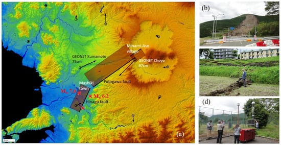
Figure 1.
(a) Locations of the causative faults of the 2016 Kumamoto earthquake sequence, GNSS stations, and Minami-Aso village on a GSI map [34]. Three ground photos taken in a field survey by the authors on 16 June 2016; (b) the largest landslide near Kawayo; (c) surface faulting in Kawayo; (d) GEONET Choyo station, where the largest horizontal movement of 97 cm was recorded.
Minami-Aso village (area: 137.3 km2, population: 11,500) is located in the western caldera of the Aso volcano. The study area includes two heavily affected districts, Kawayo and Tateno, in Minami-Aso village, as shown in the aerial photo in Figure 2, taken by the GSI on 16 April 2016, several hours after the main shock [34]. The largest landslide in the event, which caused the collapse of the Aso-Ohashi bridge, is seen in Kawayo. The eastern edge of the causative fault [31] appeared on the ground surface in Kawayo, and many wooden houses and apartment buildings collapsed in this area. Tateno district was also severely affected by strong shaking, and the failure of a water tank on the hill caused water to flow into the district [35].
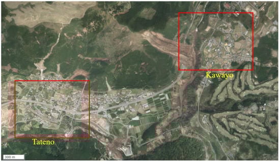
Figure 2.
Orthorectified aerial photo of the study area in Minami-Aso village, including Kawayo and Tateno districts, taken by GSI on 2016/04/16 [34].
After the earthquake, the municipal government conducted damage assessment for most of the buildings in Minami-Aso village [36] using the Japanese unified loss evaluation method [37]. A total of 4733 buildings were classified into five damage classes: Major (L4), Moderate+ (L3), Moderate- (L2), Minor (L1), and No damage (L0), where L# means the level of building damage in terms of monetary loss [37,38]. The approximate locations of building points in the damage survey were also included in the database produced by the local government. Based on the geo-location data, we manually shifted them to the building footprints of the GSI’s base map, since in some cases, the building center points in the database did not fall inside the footprints. Due to this time-consuming work, we must limit the area of the data matching to only the parts of the village (i.e., the two districts) in which the damage from the earthquake was most extensive. Since the objective of this research is the extraction of totally collapsed buildings (a part of L4 buildings), this data selection is considered not to affect the extraction result too much.
3. Multi-Temporal LiDAR Data and Optical Images for Minami-Aso Village
Pre- and post-event LiDAR data, provided by the GSI and shown in Table 1 and Figure 3, were used in this study. These datasets cover the north-western part of Minami-Aso village along the Shirakawa and Kurokawa rivers, and they were acquired by the GSI and the Ministry of Land, Infrastructure, Transport and Tourism (MLIT), Japan, for the purpose of national land surveying, disaster response, and river management. The datasets contain original random point data as well as DEMs, in which trees and buildings have been removed. Since our objective is the assessment of building damage, we processed the original random point data and produced DSMs with grids of 0.50 m or 0.25 m, including buildings and trees. Please note that the average point densities of the current datasets (5–39 points/m2) are much higher than those (1.5–4 points/m2) used in our previous studies for Mashiki town [21,22].

Table 1.
Acquisition time, average point density, and DSM spacing, and corresponding optical images of the LiDAR datasets used in this study.
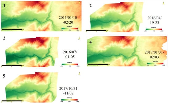
Figure 3.
DSMs of the five LiDAR datasets for the study area of Mimami-Aso village.
Figure 4 shows optical images acquired at similar times from the five LiDAR datasets. The aerial photos 1 and 5 were acquired at the same time during LiDAR surveying flights. The aerial photos 2 and 3 were obtained as part of disaster response activities by the GSI for the Kumamoto earthquake. An aerial image corresponding to LiDAR dataset 4 was not found; hence, a high-resolution satellite image from Google Earth was used as a reference optical image (only for Kawayo district).
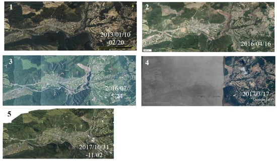
Figure 4.
Optical images acquired at similar times from the five LiDAR datasets for the study area of Mimami-Aso village.
4. Extraction of Collapsed Buildings from LiDAR Data and Their Validation
To evaluate changes in the Earth’s surface in a period of time (time i to time i + 1), the difference between the DSMs acquired at two different times can be calculated using the following equation:
The average value of the DSM difference was calculated by introducing the footprints of buildings in a GIS format. A coarser DSM spacing (Table 1) of i or i + 1 is used if they have different values.
Figure 5 shows the co-event DSM difference () for the common area of the two datasets. The earthquake-induced landslides are clearly highlighted by the dark blue color, showing the height reduction in the DSM in the main shock. In the figure, soil movement boundaries due to the earthquake, detected visually by National Research Institute for Earth Science and Disaster Resilience (NIED) [39], are also shown.
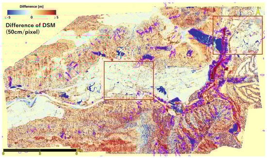
Figure 5.
DSM difference in the co-event period (2013.1–2016.4) with pixel spacing of 0.5 m. Kawayo and Tateno districts are highlighted by red squares. Pink lines show the soil movement due to the earthquake detected by NIED [39].
To extract building damage from the DSM difference, the effect of the crustal movements should be removed. For the entire area of Figure 5, the crustal movements were considered to be highly complicated [31]. Thus, we co-registered the pre- and post-event DSMs for each target area in the square.
Figure 6 shows a DSM difference in the co-event period (2013.1–2016.4) for Kawayo district compared to building footprints in the pre-earthquake period [40]. In the figure, the black square shows the location at which three wooden apartment buildings totally collapsed and human casualties were reported.
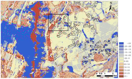
Figure 6.
DSM difference in the co-event period (2013.1–2016.4) for Kawayo district with building footprints [40]. In the black square, three apartment buildings had totally collapsed.
Figure 7 shows the DTM difference for the co-event period, produced by the GSI, whereby the trees and buildings were removed from the DSMs. In the figure, the black square shows the area in which most of the buildings in Kawayo were located. The ground level (the foundation of buildings) settled by an average of 0.5 m in the square. Hence, we added 0.5 m to the DSM difference (ΔH) for each building in Kawayo when calculating the building settlement within the footprint.
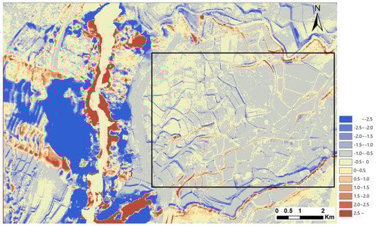
Figure 7.
DTM difference in the co-event period (2013.1–2016.4) for Kawayo district. The average value within the black square was −0.5 m.
Figure 8 shows the DSM difference in the co-event period (2013.1–2016.4) for Tateno district. In the figure, three red-circled buildings exhibited an increase in height during this period. Compared to the aerial photos in Figure 4, these buildings were confirmed to be built during the pre-event period. Thus, they were thereafter excluded from height change analysis.
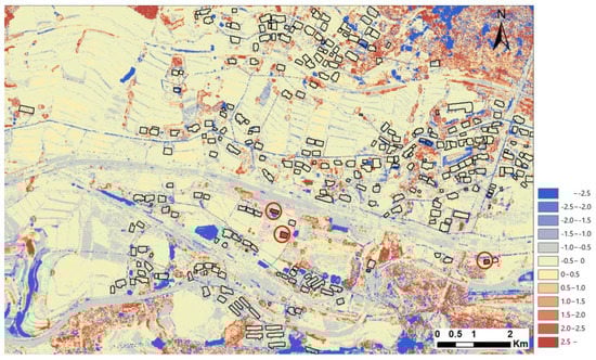
Figure 8.
DSM difference in the co-event period (2013.1–2016.4) for Tateno district with building footprints [40]. The three red-circled buildings were newly built during this period.
Figure 9 shows the DTM difference for Tateno district. In the figure, the two black squares show the area where most of the buildings were located. The ground level settled 0.7 m on average, there. Hence, we added 0.7 m to the DSM difference for each building in Tateno when calculating the settlements of the buildings.
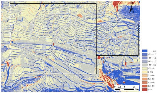
Figure 9.
DTM difference in the co-event period (2013.1–2016.4) for Tateno district. The average value within the black squares was −0.7 m.
The aerial photo on the day of the main shock (Figure 2) was enlarged for Kawayo district and is shown in Figure 10 with building footprints [40] and the damage levels supplied by the local government [36].
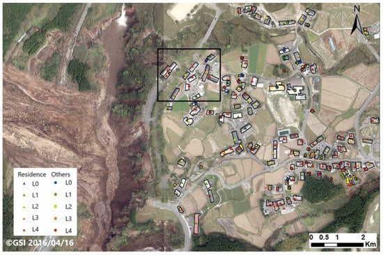
Figure 10.
Orthorectified aerial photo of Kawayo district, taken by GSI on 2016/04/16, with building footprints and damage classification provided by the local government. The triangular damage level symbols indicate residential buildings, while the circular symbols indicate non-residential buildings.
Table 2 shows the approximate relationships among the Japanese unified damage levels (L#) by the Cabinet Office of Japan [37,41], European Macroseismic Scale 1998 (EMS-98) [42], and the Okada and Takai method [43]. The monetary loss percentage is a basic index for the Japanese unified method. The first-stage assessment, viewing from outside, is conducted first. This result is shown to the residents, and in cases where they do not accept it, the second stage assessment, viewing the damage status of the inside of the building, is carried out. Conversely, EMS-98 and Okada and Takai determine the damage grade only by means of visual inspection from outside in the field [44] or from high-resolution optical images [20].
Table 2.
Earthquake loss evaluation classes of buildings used by local governments in Japan and schematic images of other damage classification methods [38].
The DSM difference between the pre- and post-event LiDAR data can be used to extract the 3D changes in a building, such as story collapse, inclination, rotation, and lateral displacement from the foundation. Hence, the damage patterns in the ESM-98 and Okada and Takai are considered to represent the DSM difference better than the monetary loss assessment [37]. Another problem with using the Japanese unified damage level is that the “Major damage (L4)” level covers such a wide range, such as from G3 to G5 (in EMS-98) and from D3 to D5 (Okada and Takai). It is considered that the DSM difference is only able to detect the damage status of apparent changes in the building shape equal to or higher than G4 or D4. In our previous study on LiDAR data for Mashiki town [22], the damage survey result [44] based on Okada and Takai was used as reference data. However, such extensive damage survey data covering a wide area do not exist for Minami-Aso village. Hence, we used the loss assessment data provided by the municipal government as reference data in this study.
Figure 11 compares the close-up of the aerial image acquired on 2016/04/29 by the GSI (Figure 11a) and the co-event DSM difference (Figure 11b) for the black square in Figure 6 and Figure 10. The damage levels are shown using color symbols in the footprints. A reduction of more than 2.0 m in the average DSM can be observed within the footprints of the collapsed apartment buildings (A–C). These three buildings were labeled as L4 (major). However, note that the major damage level also includes laterally displaced (or inclined) but still-standing buildings (such as D) and buildings with no apparent change in shape (such as E), because the definition is “more than 50% loss of the building value.” For buildings with a lower damage level (L0–L3), the change in 3D shape was difficult to recognize within their footprints.
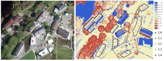
Figure 12 shows a 3D plot of the LiDAR random point data for the eight buildings (A–H) in Figure 11. Clear settlements of the red points for Dataset 2 (2016.4) compared with the blue points for Dataset 1 (2013.1) can be observed for buildings A, B, C. For building D, the heights of the two datasets look almost the same, but some shift can be seen around the footprints and roof edges. Compared with Figure 11b, building D might be shifted to the north-west from the foundation or inclined to the south-east. For the other four buildings (E–H), no clear difference can be seen between the two sets of random point data. Some differences can be seen near the outer edges of the buildings, but these might be caused by the co-registration error of the DSMs or trees or poles close to the buildings.
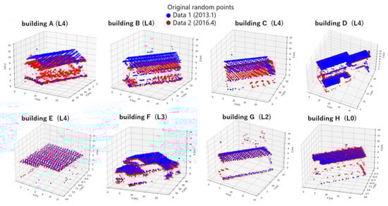
Figure 12.
A 3D plot of the random point data for eight buildings (A–H) in Figure 11. Blue points for Dataset 1 (2013.1) and red points for Dataset 2 (2016.4).
Matching of the building footprints and the building point data with damage levels was carried out for a total of 429 buildings in the Kawayo and Tateno districts. To extract buildings suffering major damage (L4) from the LiDAR DSM difference, we introduced a buffer to reduce the footprint area when taking the average of ΔH, because of the effects of trees and point density when they are close to the footprint boundary. We selected a buffer of 1.0 m, the same value as used in the previous study [22], after comparing buffer values of 0.5 and 1.0 m. Buildings with a reduced footprint area of less than 16 m2 were also excluded, because small buildings might present larger errors. A total of 396 (L0: 51, L1: 124, L2: 90, L3: 25, and L4: 106) buildings remained after performing data selection for the two districts.
Figure 13a shows the scatter plot for the 396 buildings. The average height difference within the reduced footprint (= ΔHav) and their standard deviation (σ) are plotted for the five damage levels. Please note that in our previous study [22], we also considered the correlation coefficient to be the third explanatory variable. However, it was found to be insignificant after some trials, and hence only two parameters, the average and standard deviation of ΔH within the reduced footprint, were used in this study. We expected that only a part of the L4 class would be able to be extracted from the LiDAR data, because significant height changes occur only for part of the L4 damage [45].
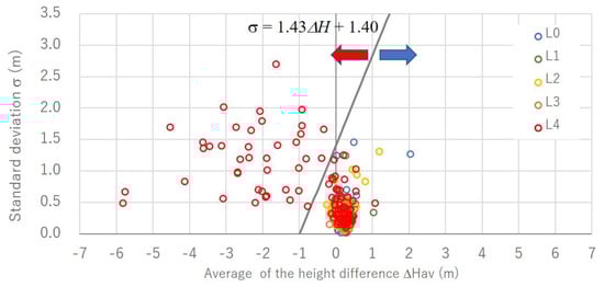
Figure 13.
The relationship between the average height difference within the reduced (−1.0 m) footprint and the standard deviation of the difference for 396 buildings with five damage levels. The division line (p = 0.5) between L4 and L0–L3 was obtained by means of logistic regression.
Logistic regression [46,47,48,49], which is suitable for representing qualitative (such as the damage level) dependent variables, was introduced in order to model the probability (p = 0.0–1.0) to fall in the major damage level (L4). Consider a two-class problem, L4 or other (i.e., L0–L3), for a given set of building damage data with m explanatory variables and the sample size N. The linear discriminant is represented as a linear combination:
where and are the vectors of the coefficients and the explanatory variables, respectively, and T denotes the transpose. The decision boundary is defined by = 0. Introducing the logistic function, the threshold classifier is determined by
where x belongs to L4 if and to L0–L3 otherwise. The unknown coefficient vector b is obtained by solving the following equations:
where is the probability that the i-th sample belongs to the L4 class. The set of Equations (4) and (5) can be solved iteratively using the maximum likelihood method to obtain the coefficient vector b.
In this study, the two explanatory variables, x1 (= ΔHav) and x2 (σ), were considered to obtain b0, b1, b2 as the regression coefficients, and they were obtained as −1.492, −1.516, 1.063 for the 396 buildings. The division line (p = 0.5) between L4 and L0–L3 was obtained as also shown in Figure 13. On the basis of this analysis, the standard deviation was found to be less influential than ΔHav when classifying L4 and the other damage levels.
Thus, we also tried a simple thresholding method using only the average difference ΔHav for extracting the L4 class. Figure 14 shows the kappa coefficient (which takes into account the possibility of the agreement occurring by chance) and the overall accuracy (simple percent agreement) using only one explanatory variable (ΔHav) and changing its threshold value in 0.1 m intervals. For the current dataset, −0.3 m gave the highest kappa value (0.44). The maximum value of the overall accuracy (0.82) was obtained for the range between −0.8 and −0.6 m.
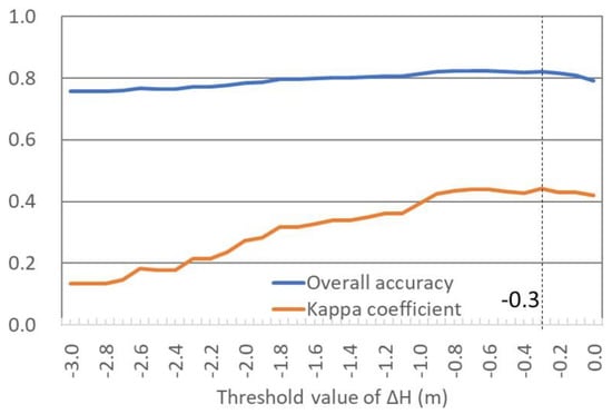
Figure 14.
The kappa coefficient and overall accuracy using only ΔHav and by changing its threshold value in 0.1 m intervals.
A similar threshold value (−0.5 m) was obtained when extracting collapsed (D5 in Okada and Takai) buildings in our previous study [22] on Mashiki town, where the damage survey results reported by Yamada et al. [44] were used as reference data. For the Amatrice earthquake [25], a settlement of −1.5 m was determined as for the upper boundary of G5 damage in the EMS-98 scale, with −0.4 m being that G4. Although there are differences with respect to the damage classification methods and the building types among the three cases, the results are in quite good agreement.
Table 3 shows the confusion matrix for the two cases: the logistic regression using the two variables, and the thresholding of ΔHav. Exactly the same results were obtained for the two cases. This fact means that the division line in Figure 13 gave the same result for the vertical line passing ΔHav = −0.3 m. Out of 396 buildings, 106 were L4 and 293 were L0–L3 in the survey data. However, only 40 L4 buildings (recall: 38%) were extracted from the LiDAR DSM difference, because only those with a settlement greater than 0.3 m met the selection criteria. Conversely, the precision was as high as 89% (40 out of 45 buildings were correctly extracted as L4). This result indicates that buildings with collapsed stories, which may result in human casualties, can be extracted accurately using pre- and post-earthquake high-density LiDAR DSM data.
Table 3.
Confusion matrix for the extraction of building suffering major (L4) damage using logistic regression and thresholding the DSM difference.
5. Monitoring of Removal Process of Damaged Buildings
Since we have the four post-event LiDAR datasets shown in Table 1, they were used to monitor the recovery process, notably the removal of damaged buildings after the main shock on 16 April 2016. The DSM differences in the three post-event periods are shown in Figure 15a–c for Kawayo district. Please note that straight lines in the figure are electric power lines used for recovery activities. It can be observed that there was almost no demolition of buildings for the three months after the earthquake. In the period from July 2016 to January 2017, many buildings shown in blue color (height reduction more than 2 m) were demolished and removed. In the next period, from January 2017 to October 2017, the demolition and removal of buildings continued. Only one footprint exhibits an increased height (red color) in this period, indicating new construction.
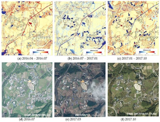
These observations on the basis of the DSM differences can also be confirmed from the optical image shown in Figure 15d–f, which is a close-up of Figure 4 (images 3–5). In the aerial images, the blue-colored footprint buildings in the DSM difference can be seen to be removed at the end of the corresponding period.
Similar plots of DSM differences and aerial images for Tateno district are shown in Figure 16. In the figure, the DSM difference and the aerial image (corresponding to either starting or ending year/month) are shown side by side for easy comparison. In the aerial photo (Figure 16b) taken on 2016/04/16, building footprints and damage levels by the local government are also shown. The removal process of buildings in Tateno took place at a similar speed to that in Kawayo. Almost no activity can be observed in the first three months until July 2016. Demolition and removal activities were accelerated in the periods until January 2017 and October 2017.
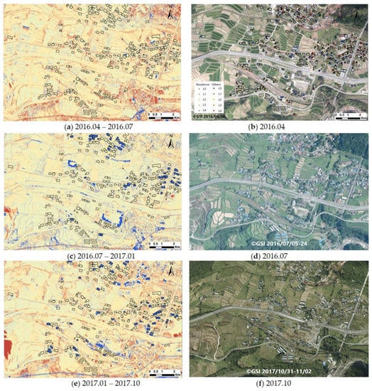
Figure 16.
DSM difference for Tateno district in the three periods after the earthquake (a,c,e), and the optical images (the close-ups of Figure 4) on three corresponding dates (b,d,f). The color chart of the DSM differences is the same as that in Figure 8. In the aerial photo (b), taken by GSI on 2016/04/16, building footprints and damage levels are also shown in the same manner as in Figure 10 for Kawayo.
We assumed that a building had been removed during the corresponding period if the average height reduction in the DSM difference within the 1 m-reduced footprint was equal to or greater than 1 m. This threshold value may be sufficient, considering the fact that a single story in ordinary Japanese houses is approximately 3 m high, and that even if a one-story building collapses, it will still have an average height greater than 1 m.
Based on this height reduction criterion, we extracted removed buildings from 396 buildings in Kawayo and Tateno district. Figure 17a shows the number of buildings removed at the end of the three periods (year/month) and the total number of buildings for the five damage levels. For example, out of 106 buildings suffering from major (L4) damage, only 6 buildings (5.7%) had been removed by July 2016, 60 (56.6%) had been removed by January 2017, and 88 (83.0%) had been removed by October 2017.
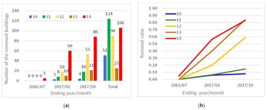
Figure 17.
(a) The number of removed buildings at the end of the period (year/month) and the total number for each damage level. (b) The ratios of removed buildings at the end of the period (year/month) for each damage level.
The ratios of removed buildings for the five damage levels are plotted in Figure 17b. It can be seen that more than 80% of L3 and L4 buildings had been removed by 1.5 years after the earthquake. It can also be noted that 58.9% of L2 buildings were also removed in 1.5 years. This fact is related to the financial support provided by local governments in Japan to cover removal costs for damaged buildings. In Minami-Aso village, the municipality supported 100% of the removal costs if houses or commercial buildings owned by small businesses were judged to be equal to or higher than L2-level damage [50].
Conversely, the removal ratios were lower for less damaged buildings (L1: 14.5%, L0: 7.8%). All these values are higher than those in Nishinomiya city (L4: 67.0%; L3 and L2: 21.5%; L1 and L0: 5.5%) after the 1995 Kobe earthquake [51]. In the municipalities affected by the Kobe earthquake, similar financial support was given to their residents. Thus, the damage classification results provided by the municipal governments can be considered to affect the judgments of owners regarding the demolition and removal of damaged buildings.
6. Discussion on the Use of LiDAR Data in Disaster Management
LiDAR data are considered to be very useful for acquiring 3D models of various objects on the surface of the Earth. However, it is still costly to acquire observations covering a wide area at ordinary (i.e., pre-disaster) times. Hence, the direct comparison of pre- and post-event LiDAR data often encounters difficulties due to the lack of pre-event data. Even if pre-event data exist, they are sometimes old or have a low point density. However, high-density and frequent LiDAR observations are often carried out by geospatial data agencies, such as the GSI in Japan. They perform LiDAR surveying flights regularly, at intervals of several (5 to 10) years, especially for developing DTMs for national land maps and building footprint data. It was fortunate that we were able to use very valuable LiDAR data covering one of the most severely affected areas, Minami-Aso village, with high density and high frequency. We also searched for post-event LiDAR data for Mashiki town, but could not find them in the recovery stage.
To perform the damage assessment of buildings from LiDAR DSMs, building footprint data are also necessary. Otherwise, the effects of seasonal changes in trees/agricultural fields and parking/moving vehicles are significant for the extraction of changes due to disasters. These days, building footprint data are available from open sources, such as OpenStreetMap, and their use is also possible in some cases, but they are not so accurate in Japan, nor do they have wide coverage. Fortunately, the GSI recently developed the fundamental GIS map [40] with building footprints for most urban areas in Japan, and thus we were able to use it in this study.
If the pre-event LiDAR data are not available, the use of other remote sensing data, such as high-resolution optical and SAR satellite images, airborne optical and SAR images, and UAV images, is possible either for developing a pre-event building 3D model or for extracting damage status through their combined use [52]. To validate the results from pre- and post-event LiDAR data, those remote sensing data are highly useful. Of course, if we use the pre- and post-event LiDAR data and other remote sensing or GIS data together, the accuracy of change (change) detection will increase.
As already discussed in the previous chapters, damage classification data obtained as a result of field investigations are quite important for validating the extraction results from LiDAR data. Damage classification methods depend on the objectives of surveys, and thus, suitable validation data are not always available. Local governments in Japan issue disaster victim certificates [37] to all citizens if their houses have been affected by natural disasters. Such survey data cover severely affected areas, and they are thus suitable for developing building fragility curves [38,49]. However, as the validation data of remote sensing imagery, they include minor damage status, which is difficult to observe from external views; hence, simple field investigation data from outside [42,43,44] are a better reference if they exist.
Multi-temporal LiDAR data can also be used for landslide mapping or ground failure monitoring [24]. We will show such results for the Minami-Aso region in the near future. Finally, we should insist on the necessity of continuous monitoring of stricken areas from natural disasters. Disaster resilience [53] is becoming an important concept for coping with natural hazards in the world.
7. Conclusions
The use of multi-temporal LiDAR data was explored for extracting collapsed buildings and monitoring their removal process in Minami-Aso village, Kumamoto prefecture, Japan, after the 2016 Kumamoto earthquake. The difference in the digital surface models (DSMs) acquired at pre- and post-event times within the building footprints was employed to identify collapsed buildings, and the results were compared with damage survey data provided by the municipal government and aerial optical images. Approximately 40% of severely damaged (L4) buildings showed a reduction in their average height within a 1 m-reduced building footprint for the co-event DSM difference. The reason for the low extraction rate is that the major damage level (L4) used in the field survey includes a wide range of damage patterns, from totally collapsed to damaged but still standing. The demolition and removal process of the affected buildings was also monitored using the differences in DSM at three post-event time points. More than 80% of L4 and L3 (moderate+) buildings were removed by 1.5 years after the earthquake, approximately 60% of buildings at the L2 (moderate−) level, and less than 15% for the lower damage levels (L1 and L0). The high removal ratio of L2 damage (20% to 40% monetary loss ratio) buildings was probably partially a result of the full support for removal costs provided by the local government. Thus, the official damage classification result was found to influence judgements by the owners regarding the demolition and removal of damaged buildings. As shown in this research, multi-temporal LiDAR data are quite useful for observing three-dimensional changes in buildings in all phases of the disaster cycle.
Author Contributions
Conceptualization, F.Y. and W.L.; validation, F.Y. and W.L.; formal analysis, W.L.; investigation, F.Y.; resources, F.Y.; data curation, F.Y. and K.H.; writing—original draft preparation, F.Y.; writing—review and editing, F.Y., W.L. and K.H.; visualization, W.L.; supervision, F.Y.; project administration, F.Y.; funding acquisition, F.Y. All authors have read and agreed to the published version of the manuscript.
Funding
This research was partially funded by JSPS KAKENHI Grant Number 21H01598, Japan.
Data Availability Statement
Not applicable.
Acknowledgments
The five-temporal LiDAR datasets used in this study were provided by the GSI through agreement with the National Research Institute for Earth Science and Disaster Resilience (NIED). The building damage classification data were made available from Minami-Aso village to the research program of NIED aiming at recovery support.
Conflicts of Interest
The authors declare no conflict of interest.
Abbreviation
A list of the used abbreviations:
| CAD | Computer-Aided Design |
| DEM | Digital Elevation Model |
| DSM | Digital Surface Model |
| DTM | Digital Terrain Model |
| ESM-98 | European Macroseismic Scale 1998 |
| GEONET | The Japanese National GNSS Earth Observation Network System |
| GIS | Geographic Information System |
| GNSS | Global Navigation Satellite System |
| GSI | Geospatial Information Authority of Japan |
| JST | The Japan Standard Time |
| LiDAR | Light Detection and Ranging |
| NIED | National Research Institute for Earth Science and Disaster Resilience |
| SfM | Structure-from-Motion |
| UAV | Unmanned Aerial Vehicle |
References
- Rathje, E.; Eeri, M.; Adams, B.J. The role of remote sensing in earthquake science and engineering: Opportunities and challenges. Earthq. Spectra 2008, 24, 471–492. [Google Scholar] [CrossRef]
- Ghaffarian, S.; Kerle, N.; Filatova, T. Remote sensing-based proxies for urban disaster risk management and resilience: A review. Remote Sens. 2018, 10, 1760. [Google Scholar] [CrossRef]
- Dell’Acqua, F.; Gamba, P. Remote sensing and earthquake damage assessment: Experiences, limits, and perspectives. Proc. IEEE 2012, 100, 2876–2890. [Google Scholar] [CrossRef]
- Dong, L.; Shan, J. A comprehensive review of earthquake-induced building damage detection with remote sensing techniques. ISPRS J. Photogramm. Remote Sens. 2013, 84, 85–99. [Google Scholar] [CrossRef]
- Qin, R.; Tian, J.; Reinartz, P. 3D change detection—Approaches and applications. ISPRS J. Photogramm. Remote Sens. 2016, 122, 41–56. [Google Scholar] [CrossRef]
- Guth, P.L.; Van Niekerk, A.; Grohmann, C.H.; Muller, J.-P.; Hawker, L.; Florinsky, I.V.; Gesch, D.; Reuter, H.I.; Herrera-Cruz, V.; Riazanoff, S.; et al. Digital Elevation Models: Terminology and Definitions. Remote Sens. 2021, 13, 3581. [Google Scholar] [CrossRef]
- Štular, B.; Lozić, E.; Eichert, S. Airborne LiDAR-Derived Digital Elevation Model for Archaeology. Remote Sens. 2021, 13, 1855. [Google Scholar] [CrossRef]
- Maruyama, Y.; Tashiro, A.; Yamazaki, F. Detection of collapsed buildings due to earthquakes using a Digital Surface Model constructed from aerial images. J. Earthq. Tsunami 2014, 8, 1450003. [Google Scholar] [CrossRef]
- Susaki, J. Region-based automatic mapping of tsunami-damaged buildings using multi-temporal aerial images. Nat. Hazards 2015, 76, 397–420. [Google Scholar] [CrossRef][Green Version]
- Westoby, M.; Brasington, J.; Glassera, N.; Hambrey, M.; Reynolds, J. ‘Structure-from-Motion’ photogrammetry: A low-cost, effective tool for geoscience applications. Geomorphology 2012, 179, 300–314. [Google Scholar] [CrossRef]
- Cheng, M.L.; Matsuoka, M.; Liu, W.; Yamazaki, F. Near-real-time gradually expanding 3D land surface reconstruction in disaster areas by sequential drone imagery. Autom. Constr. 2022, 135, 104105. [Google Scholar] [CrossRef]
- Fernandez Galarreta, J.; Kerle, N.; Gerke, M. UAV-based urban structural damage assessment using object-based image analysis and semantic reasoning. Nat. Hazards Earth Syst. Sci. 2015, 15, 1087–1101. [Google Scholar] [CrossRef]
- Yamazaki, F.; Kubo, K.; Tanabe, R.; Liu, W. Damage assessment and 3D modeling by UAV flights after the 2016 Kumamoto, Japan earthquake. In Proceedings of the 2017 IEEE International Geoscience and Remote Sensing Symposium, Fort Worth, TX, USA, 23–28 July 2017; pp. 3182–3185. [Google Scholar] [CrossRef]
- Murakami, H.; Nakagawa, K.; Hasegawa, H.; Shibata, T.; Iwanami, E. Change detection of buildings using an airborne laser scanner. ISPRS J. Photogramm. Remote Sens. 1999, 54, 148–152. [Google Scholar] [CrossRef]
- Vu, T.T.; Matsuoka, M.; Yamazaki, F. LIDAR-based change detection of buildings in dense urban areas. In Proceedings of the 2004 IEEE International Geoscience and Remote Sensing Symposium, Anchorage, AK, USA, 20–24 September 2004; pp. 3413–3416. [Google Scholar] [CrossRef]
- Xu, H.; Cheng, L.; Li, M.; Chen, Y.; Zhong, L. Using Octrees to detect changes to buildings and trees in the urban environment from airborne LiDAR data. Remote Sens. 2015, 7, 9682–9704. [Google Scholar] [CrossRef]
- Wang, X.; Li, P. Extraction of urban building damage using spectral, height and corner information from VHR satellite images and airborne LiDAR data. ISPRS J. Photogramm. Remote Sens. 2020, 159, 322–326. [Google Scholar] [CrossRef]
- He, M.; Zhu, Q.; Du, Z.; Hu, H.; Ding, Y.; Chen, M. A 3D shape descriptor based on contour clusters for damaged roof detection using airborne LiDAR point clouds. Remote Sens. 2016, 8, 189. [Google Scholar] [CrossRef]
- Corbane, C.; Saito, K.; Dell’Oro, L.; Bjorgo, E.; Gill, S.P.; Piard, B.E.; Huyck, C.K.; Kemper, T.; Lemoine, G.; Spence, R.J.; et al. A Comprehensive Analysis of Building Damage in the 12 January 2010 Mw7 Haiti Earthquake Using High-Resolution Satellite and Aerial Imagery. Photogramm. Eng. Remote Sens. 2011, 77, 997–1009. [Google Scholar] [CrossRef]
- Miura, H.; Midorikawa, S.; Matsuoka, M. building damage assessment using high-resolution satellite SAR images of the 2010 Haiti Earthquake. Earthq. Spectra 2016, 32, 591–610. [Google Scholar] [CrossRef]
- Moya, L.; Yamazaki, F.; Liu, W.; Chiba, T. Calculation of coseismic displacement from lidar data in the 2016 Kumamoto, Japan, earthquake. Nat. Hazards Earth Syst. Sci. 2017, 17, 143–156. [Google Scholar] [CrossRef]
- Moya, L.; Yamazaki, F.; Liu, W.; Yamada, M. Detection of collapsed buildings from lidar data due to the 2016 Kumamoto earthquake in Japan. Nat. Hazards Earth Syst. Sci. 2018, 18, 165–178. [Google Scholar] [CrossRef]
- Hajeb, M.; Karimzadeh, S.; Matsuoka, M. SAR and LIDAR datasets for building damage evaluation based on Support Vector Machine and Random Forest algorithms—A case study of Kumamoto Earthquake, Japan. Appl. Sci. 2020, 10, 8932. [Google Scholar] [CrossRef]
- Liu, W.; Yamazaki, F.; Maruyama, Y. Detection of earthquake-induced landslides during the 2018 Kumamoto Earthquake using multitemporal airborne Lidar data. Remote Sens. 2019, 11, 2292. [Google Scholar] [CrossRef]
- Zhou, Z.; Gong, J.; Hu, X. Community-scale multi-level post-hurricane damage assessment of residential buildings using multi-temporal airborne LiDAR data. Autom. Constr. 2019, 98, 30–45. [Google Scholar] [CrossRef]
- Saganeiti, L.; Amato, F.; Nol‘e, G.; Vona, M.; Murgante, B. Early estimation of ground displacements and building damage after seismic events using SAR and LiDAR data: The case of the Amatrice earthquake in central Italy, on 24th August 2016. Int. J. Disaster Risk Reduct. 2020, 51, 101924. [Google Scholar] [CrossRef]
- Meslem, A.; Yamazaki, F.; Maruyama, Y.; Benouar, D.; Kibboua, A.; Mehani, Y. The effects of building characteristics and site conditions on the damage distribution in Boumerdes after the 2003 Algeria earthquake. Earthq. Spectra 2012, 28, 185–216. [Google Scholar] [CrossRef]
- Hoshi, T.; Murao, O.; Yoshino, K.; Yamazaki, F.; Estrada, M. Post-disaster urban recovery monitoring in Pisco after the 2007 Peru earthquake using satellite image. J. Disaster Res. 2014, 9, 1059–1068. [Google Scholar] [CrossRef]
- Hashemi-Parast, S.O.; Yamazaki, F.; Liu, W. Monitoring and evaluation of the urban reconstruction process in Bam, Iran, after the 2003 Mw6.6 earthquake. Nat. Hazards 2017, 85, 197–213. [Google Scholar] [CrossRef]
- Yamazaki, F.; Liu, W. Remote sensing technologies for post-earthquake damage assessment: A case study on the 2016 Kumamoto earthquake, Keynote Lecture. In Proceedings of the 6th Asia Conference on Earthquake Engineering, Cebu City, Philippines, 22–24 September 2016. [Google Scholar]
- Shirahama, Y.; Yoshimi, M.; Awata, Y.; Maruyama, T.; Azuma, T.; Miyashita, Y.; Mori, H.; Imanishi, K.; Takeda, N.; Ochi, T.; et al. Characteristics of the surface ruptures associated with the 2016 Kumamoto earthquake sequence, central Kyushu, Japan. Earth Planets Space 2016, 68, 191. [Google Scholar] [CrossRef]
- Yamazaki, F.; Liu, W. Recovery monitoring of Minami-Aso area after the 2016 Kumamoto earthquake based on remote sensing data. In Proceedings of the 8th Asia Conference on Earthquake Engineering, Taipei, Taiwan, 9–11 November 2022. [Google Scholar]
- Liu, W.; Yamazaki, F. Extraction of collapsed buildings due to the 2016 Kumamoto earthquake based on multi-temporal PALSAR-2 data. J. Disaster Res. 2017, 12, 241–250. [Google Scholar] [CrossRef]
- Geospatial Information Authority of Japan (GSI). Information on the 2016 Kumamoto Earthquake (in Japanese). Available online: http://www.gsi.go.jp/BOUSAI/H27-kumamoto-earthquake-index.html (accessed on 1 October 2022).
- Kyushu Electric Power Co., Inc. Damage to Hydropower Facilities (in Japanese). Available online: https://www.meti.go.jp/shingikai/sankoshin/hoan_shohi/denryoku_anzen/denki_setsubi/pdf/011_06_00.pdf (accessed on 1 October 2022).
- Minami-Aso Village. Recovery Report from the 2016 Kumamoto Earthquake. 2022. (In Japanese). Available online: https://www.amazon.co.jp/%E5%B9%B3%E6%88%9028%E5%B9%B4%E7%86%8A%E6%9C%AC%E5%9C%B0%E9%9C%87-%E5%8D%97%E9%98%BF%E8%98%87%E6%9D%91%E7%81%BD%E5%AE%B3%E8%A8%98%E9%8C%B2%E8%AA%8C-%E5%8D%97%E9%98%BF%E8%98%87%E6%9D%91-ebook/dp/B07B4XD5PZ?asin=B07B4XD5PZ&revisionId=&format=4&depth=1.l (accessed on 1 October 2022).
- Cabinet Office of Japan. Operational Guideline for Damage Assessment of Residential Buildings in Disasters (in Japanese). Available online: http://www.bousai.go.jp/taisaku/pdf/h3003shishin_all.pdf (accessed on 1 October 2022).
- Yamazaki, F.; Suto, T.; Liu, W.; Matsuoka, M.; Horie, K.; Kawabe, K.; Torisawa, K.; Inoguchi, M. Development of fragility curves of Japanese buildings based on the 2016 Kumamoto earthquake. In Proceedings of the 2019 Pacific Conference on Earthquake Engineering, Auckland, New Zealand, 4–6 April 2019. [Google Scholar]
- National Research Institute for Earth Science and Disaster Resilience (NIED). Soil Movement by the Kumamoto Earthquake (in Japanese). Available online: http://www.bosai.go.jp/mizu/dosha.html (accessed on 1 October 2022).
- Geospatial Information Authority of Japan (GSI). Download Service of Fundamental Map Information (in Japanese). Available online: https://fgd.gsi.go.jp/download/mapGis.php (accessed on 1 October 2022).
- Tanaka, S.; Shigekawa, K. Development of training system for building damage assessment using actual buildings. J. Disaster Res. 2014, 9, 188–197. [Google Scholar] [CrossRef]
- ESC, Working Group Macroseismic Scales. European Macroseismic Scale 1998 (EMS-98); Grünthal, G., Ed.; European Seismological Commission, Subcommission on Engineering Seismology: Luxembourg, 1998; Volume 15, Available online: https://www.franceseisme.fr/EMS98_Original_english.pdf (accessed on 5 October 2022).
- Okada, S.; Takai, N. Classifications of structural types and damage patterns of buildings for earthquake field investigation. In Proceedings of the 12th World Conference on Earthquake Engineering, Auckland, New Zealand, 30 January–4 February 2000. [Google Scholar]
- Yamada, M.; Ohmura, J.; Goto, H. Wooden building damage analysis in Mashiki town for the 2016 Kumamoto earthquakes on April 14 and 16. Earthq. Spectra 2017, 33, 1555–1572. [Google Scholar] [CrossRef]
- Kawabe, K.; Horie, K.; Inoguchi, M.; Matsuoka, M.; Torisawa, K.; Liu, W.; Yamazaki, F. Extraction of story-collapsed buildings by the 2016 Kumamoto earthquake using deep learning. In Proceedings of the 17th World Conference on Earthquake Engineering, 9c-0021, Sendai, Japan, 27 September–2 October 2021. [Google Scholar]
- Ioannou, I.; Rossetto, T.; Grant, D. Use of regression analysis for the construction of empirical fragility curves. In Proceedings of the 15th World Conference on Earthquake Engineering, Lisbon, Portugal, 24–28 September 2012. [Google Scholar]
- Wiesberg, S. Applied Linear Regression, 4th ed.; John Wiley: New York, NY, USA, 2014; pp. 270–289. [Google Scholar]
- Moya, L.; Marval Perez, L.R.; Mas, E.; Adriano, B.; Koshimura, S.; Yamazaki, F. Novel unsupervised classification of collapsed buildings using satellite imagery, hazard scenarios and fragility functions. Remote Sens. 2018, 10, 296. [Google Scholar] [CrossRef]
- Miano, A.; Jalayer, F.; Forte, G.; Santo, F. Empirical fragility assessment using conditional GMPE-based ground shaking fields: Application to damage data for 2016 Amatrice Earthquake. Bull. Earthq. Eng. 2020, 18, 6629–6659. [Google Scholar] [CrossRef]
- Minami-Aso Village. Procedure of the Financial Support for Demolition and Removal Costs of Damaged Buildings due to the Kumamoto Earthquake (in Japanese). August 2016. Available online: https://www.vill.minamiaso.lg.jp/reiki_int/reiki_honbun/r091RG00000833.html (accessed on 5 October 2022).
- Maki, N.; Horie, K.; Hayashi, H. How many repairable houses were demolished? Debris management of the 1995 Kobe Earthquake. J. Archit. Plan. 2016, 81, 2723–2729. (In Japanese) [Google Scholar] [CrossRef][Green Version]
- Khodaverdi, N.; Rastiveis, H.; Jouybari, A. Combination of post-earthquake LiDAR data and satellite imagery for buildings damage detection. Earth Obs. Geomat. Eng. 2019, 3, 12–20. [Google Scholar] [CrossRef]
- Sakurai, M.; Shaw, R. Emerging Technologies for Disaster Resilience: Practical Cases and Theories; Springer: Singapore, 2021. [Google Scholar]


Publisher’s Note: MDPI stays neutral with regard to jurisdictional claims in published maps and institutional affiliations. |
© 2022 by the authors. Licensee MDPI, Basel, Switzerland. This article is an open access article distributed under the terms and conditions of the Creative Commons Attribution (CC BY) license (https://creativecommons.org/licenses/by/4.0/).