Article

Gaussian Process Modeling of In-Season Physiological Parameters of Spring Wheat Based on Airborne Imagery from Two Hyperspectral Cameras and Apparent Soil Electrical Conductivity

by
Wiktor R. Żelazny
1,2,*,
Krzysztof Kusnierek
3 and
Jakob Geipel
3
1
Division of Crop Management Systems, Crop Research Institute Praha-Ruzyně, Drnovská 507/73, 161 06 Praha, Czech Republic
2
Faculty of Engineering, Czech University of Life Sciences Prague, Kamýcká 129, 165 00 Praha, Czech Republic
3
Department of Agricultural Technology, Norwegian Institute of Bioeconomy Research, Pb 115, 1431 Ås, Norway
*
Author to whom correspondence should be addressed.
Remote Sens. 2022, 14(23), 5977; https://doi.org/10.3390/rs14235977
Submission received: 28 September 2022 / Revised: 16 November 2022 / Accepted: 18 November 2022 / Published: 25 November 2022
(This article belongs to the Special Issue Pattern Recognition in Hyperspectral Remote Sensing)

Abstract

:
The remote sensing of the biophysical and biochemical parameters of crops facilitates the preparation of application maps for variable-rate nitrogen fertilization. According to comparative studies of machine learning algorithms, Gaussian process regression (GPR) can outperform more popular methods in the prediction of crop status from hyperspectral data. The present study evaluates GPR model accuracy in the context of spring wheat dry matter, nitrogen content, and nitrogen uptake estimation. Models with the squared exponential covariance function were trained on images from two hyperspectral cameras (a frenchFabry–Pérot interferometer camera and a push-broom scanner). The most accurate predictions were obtained for nitrogen uptake ( R 2 = 0.75 0.85 , RPD P = 2.0 2.6 ). Modifications of the basic workflow were then evaluated: the removal of soil pixels from the images prior to the training, data fusion with apparent soil electrical conductivity measurements, and replacing the Euclidean distance in the GPR covariance function with the spectral angle distance. Of these, the data fusion improved the performance while predicting nitrogen uptake and nitrogen content. The estimation accuracy of the latter parameter varied considerably across the two hyperspectral cameras. Satisfactory nitrogen content predictions ( R 2 > 0.8 , RPD P > 2.4 ) were obtained only in the data-fusion scenario, and only with a high spectral resolution push-broom device capable of capturing longer wavelengths, up to 1000 n m , while the full-frame camera spectral limit was 790 n m . The prediction performance and uncertainty metrics indicated the suitability of the models for precision agriculture applications. Moreover, the spatial patterns that emerged in the generated crop parameter maps accurately reflected the fertilization levels applied across the experimental area as well as the background variation of the abiotic growth conditions, further corroborating this conclusion.

1. Introduction

With nitrate groundwater pollution remaining a problem in many cropland regions, it is in the public interest that variable-rate nitrogen fertilization technology continues to be developed and disseminated [1]. Although financial incentives for crop farmers—small-scale farmers managing uniform fields in particular—are currently limited [1], higher fertilizer prices caused by the increasing instability of global supply chains [2,3], and new production subsidies or taxes targeted at the overfertilization problem [1] may motivate growers toward the quicker adoption of this technology in the coming years. While nitrogen content can inform farmers about crop nutrient stress, crop biomass density needs to be considered when recommending target fertilizer rates to account for the nitrogen dilution phenomenon [4,5].
In-season canopy reflectance measurements can inform farmers about the biophysical and biochemical parameters of crops and their spatial variability in the field. Fertilizer application maps are derived from measurements to improve nitrogen-use efficiency while maintaining the satisfactory yield and quality of the crop [6,7]. Remote data acquisition with imaging sensors can provide more comprehensive information on crop parameter distribution in terms of coverage continuity, revisit frequency, and the range of detectable spatial features than proximal sensing with hand-held or tractor-mounted devices [8], especially if unmanned aerial vehicles (UAVs) are employed as sensor platforms [9,10,11].
Vegetation indices have been widely employed to map crop status based on multispectral data [7]. However, since spectral measurements are related to crop parameter values in a non-linear fashion and the saturation problem can be encountered in vegetation index applications, more powerful machine learning methods are preferred wherever the available data are of sufficient quality [12,13]. Unlike vegetation indices, machine learning makes full use of the measured spectrum, and therefore, it is particularly suited to hyperspectral data [14].
Partial least squares, random forest, and support vector regression have been commonly included in studies that compare the performance of multiple machine learning methods in the crop parameter prediction context [12,15,16,17,18,19]. All of these methods can be classified as empirical and non-parametric, with training data determining the functional relationships between input and output values in a fashion abstracted away from the physical laws [20]. Partial least squares regression is a method involving linear combinations of latent variables, each of which comprises a linear combination of input features [21]. The algorithm has low computational complexity and can readily be applied to datasets exhibiting multicollinearity, as is typical for spectral datasets. On the other hand, its linear nature constrains the predictive power of trained models [20,22]. Random forest regression is a tree-based method. As such, it enables the modeling of variable interactions. Given that each tree is trained on a bootstrap sample of data and the method has an ensemble character, a random forest is robust to overfitting and is not readily influenced by outlier observations [23]. On the other hand, the algorithm does not address input data collinearity, and the discrete within-tree decisions can lead to abrupt changes in the predicted values. Kernel-based methods enable the continuous treatment of non-linear relationships by the mapping of input features to higher-dimensional space [20]. In this group of algorithms, support vector regression exploits the concept of support vectors, which are a subset of the training observations associated with sufficient prediction errors to be accounted for in regression fitting, while data points with small errors are ignored [22]. The advantages and disadvantages of support vector regression in relation to dealing with spectral data are similar to those of random forests [20].
Similar to support vector regression, Gaussian process regression (GPR) also belongs to the class of non-parametric kernel-based algorithms [20]; however, the modeling is performed within the Bayesian statistical framework [24]. The publications of Rasmussen [25] and Schulz et al. [26] offer a gentle introduction to Gaussian processes. Briefly, a Gaussian process is a distribution over functions. This distribution is parametrized using a mean, often assumed to be zero, and a covariance function, also called a kernel—a vector of infinite length with a matrix containing infinite numbers of rows and columns. Their contents are characterized using equations, typically with hyperparameters, and actual modeling involves finite subsets of these objects. Functions can be drawn at random from a Gaussian process—these are described using a finite number of input–output pairs, rather than analytically—and at the core of the method is the assumption that the drawn outputs follow a joint Gaussian distribution. These are Bayesian priors, and during model training, their values are updated in order to not conflict with the information in the training data. Simultaneously, hyperparameters are tuned. Model predictions can be generated for new data points when the posterior Gaussian process is joined with new input data.
Flexibility [27], a reduced risk of overfitting even with modest numbers of highly dimensional observations [12,28], and extensibility [12] have been cited as the advantages of GPR in the context of crop parameter estimation. However, its major appeal, distinguishing GPR from support vector regression and other non-parametric methods, is the fact that each of the obtained predictions comes with an uncertainty estimate [10,12,29]. According to Verrelst et al. [20], this makes GPR particularly suited to vegetation property-mapping applications. The method has been employed to predict crop biophysical parameters, such as biomass density [30,31], leaf area index (LAI) [12,18,27,29,31,32], fractional vegetation cover [12,27,32], and emergence rate [10], as well as biochemical parameters, such as water content [29], chlorophyll content [12,27,29,32], nitrogen content [14,30,33], and nitrogen uptake [5,30]. A number of studies have reported that GPR performs better than other machine learning algorithms, such as partial least squares [12,18], principal components regression [18], random forests [12,18] and other tree-based methods [10,18], support vector machines [10,12,18], artificial neural networks [32], and kernel ridge regression [12]. Still, GPR has not been as extensively tested on different datasets as non-Bayesian methods, particularly partial least squares regression.
A covariance function of a Gaussian process describes in statistical terms the properties of the prior and posterior functions, in particular the similarity of outputs for a given distance of data points in the input space [26]. Camps-Valls et al. [24] and Schulz et al. [26] presented a sample of kernels employed in machine learning and demonstrated how a complex kernel can be constructed as an algebraic combination of simpler kernels. They noted that the squared exponential covariance function (SE), also known as the radial basis function, is the most common choice among GPR practitioners. It was reported by various authors [16,32,34] to provide satisfactory predictions of crop biophysical and biochemical parameters. However, Gewali and Monteiro [35] developed a modification of this kernel, in which the Euclidean distance is replaced with a spectral angle, resulting in a formulation called the exponential spectral angle mapper covariance function (ESAM). They argued that it was better suited to spectral data due to its ability to separate spectral signature shape information from magnitude information, the latter of which can be considered a nuisance component. Although their proposition is compelling, it appears that the only published follow-up studies are by the same authors [12,36,37], and only the latest publication is devoted to crop parameter estimation.
Typically, ancillary data are added to build comprehensive robust models; they include weather, soil, and crop management data. For testing single-field and single-season applications, soil data are the most relevant. Soil properties have a strong influence on crop properties [4,38], and can provide a more complete picture of spatial variability in remote sensing applications [39]. If imagery with high spatial resolution is available, the occurrence of spectra corresponding to soil pixels can inform users about crop biophysical parameters, such as gaps in the canopy related to impaired vigor. However, when spectral signatures are aggregated over a larger area to match the spatial resolution of the ground truth observations, they can also introduce noise and reduce the prediction performance [40]. Studies devoted to the spatial aggregation problem involve broadband measurements [40,41,42] or are focused on proximal sensing and vegetation indices [14,43], while the issue remains underexplored for machine learning models trained using hyperspectral data acquired with a UAV.
Even in the absence of a plant canopy to hinder the view, an airborne reflectance sensor cannot penetrate a soil block down to the rhizosphere and acquire spectral information to determine soil nutrient availability. In a variable nitrogen fertilization study, Heiẞ et al. [44] proposed combining proximal reflectance measurements with apparent soil electrical conductivity ( EC a ) data as a proxy of soil fertility. Similar sensor data fusions were evaluated in the context of soil property determination [45,46]. In an attempt to map wheat disease severity based on multispectral satellite data, Franke and Menz [47] employed measurements from a soil EC a meter to verify that the soil conditions were relatively uniform and, thus, did not cause strong variation in abiotic stress factors that would have introduced noise to the infection signal. Although EC a can be affected by a range of soil properties, including nuisance variables [38], a ground conductivity meter can penetrate the root zone, overcoming the limitations of an airborne imager. Moreover, an arbitrary spatial sampling density can readily be employed to reduce the data resolution mismatch relative to acquisitions involving a UAV.
The focus of the present study is to evaluate the performance of GPR models employed for the mapping of spring wheat dry biomass, nitrogen content, and nitrogen uptake based on airborne hyperspectral imagery acquired at the onset of the booting stage. Data collected with two hyperspectral cameras are analyzed: a full-frame device with a Fabry–Pérot interferometer (FPI) and a push-broom imager with dispersion grating. We are not aware of prior studies comparing the performance of two hyperspectral VIS-NIR imagers for airborne crop parameter estimation.
We were interested in obtaining a sufficient prediction quality for precision agriculture applications, variable-rate fertilization in particular. We show the potential of the method to improve predictions over the application of the normalized difference red edge vegetation index (NDRE) and to indicate areas with uncertain predictions while comparing the camera performance. Three strategies hypothesized to influence model quality were also tested, both alone and in combination: (1) we replaced the SE GPR kernel with the ESAM kernel, and expected an improvement in estimation accuracy; (2) we explored the effect of soil pixel removal prior to spectra aggregation and training of the models; and (3) we augmented the spectral dataset with EC a measurements, hypothesizing that the additional information would improve the models.

2. Materials and Methods

2.1. Experimental Site

The experimental field was located in Hoff, Innlandet county, Norway (60.68°N, 10.85°E; 240–250 m a.s.l.). The field has a southern exposure, with an inclination of approximately 6°. The climate is of the warm-summer humid continental Köppen type, with mean annual temperature of 3.6 °C, and mean annual precipitation sum of 600 m m , as measured at a local weather station (1991–2020). The soil is endostagnic Cambisol of moraine till origin with loam and silty sand texture. Due to undulating topography, erosion processes occur in the field, transporting clay particles and organic matter toward lower terrain. A water-holding capacity gradient is also detectable. This leads to considerable within-field variability in soil fertility.
An experimental area measuring 120   ×   100   m was delimited in the field, and divided into sixty 10   ×   10   m plot pairs, each pair spanning two rows of the area, one for biomass and one for yield (Figure 1), the latter of which was not analyzed in this study. Spring wheat cv. ‘Bjarne’ was sown on the 18 May 2018 at a rate of 235 kg ha −1 with a basal application of NPK fertilizer (22:3:10). The absolute fertilizer rate was varied across the plot columns to obtain high crop status variation on a relatively small area. There were three fertilization levels, corresponding to 40, 70 and 100 kg N ha −1. The emergence rate was high (80–100%) despite low precipitation in May (Figure 2). Damage by deer was noted late in May, but was restricted to small areas. Weeds were suppressed with a herbicide on 17 June, at the BBCH32 [48] growth stage.

2.2. Hyperspectral Data Acquisition and Pre-Processing

The hyperspectral imaging campaign was performed on 27 June 2018. The date corresponded to the crop growth stages between BBCH37 and BBCH55, depending on the experimental plot, with most of the plots in the BBCH39 growth stage. The day before, the plot borders were mowed. Five 1   ×   1   m checkered-pattern ground control points (one by each corner and one in the center of the experimental area) were placed for georeferencing, and a 50% reflectance 50   ×   50   c m Zenith Lite™ panel (Sphere Optics, Herrsching, Germany) with Zenith Polymer® coating was placed on a leveled tripod, also in the center. Downwelling irradiance was measured at 1 s intervals with an ASD FieldSpec 3 spectroradiometer (Analytical Spectral Devices Inc., Boulder, CO, USA) equipped with a remote cosine receptor placed at the northern edge of the experimental area.
Canopy spectra were captured using two hyperspectral cameras (Table 1). The first device was Rikola HSI (Rikola Ltd., Oulu, Finland), a full-frame FPI camera with sequential band capture. It was carried by a Spreading Wings S1000+ UAV (DJI, Shenzhen, China), and the imagery was acquired around 11:00 local time. The second imager was HySpex Mjolnir V-1240 (Norsk Elektro Optikk AS, Skedsmokorset, Norway), carried by Camflight FX8 (Nordic Unmanned AS, Sandnes, Norway) around 12:00. Mjolnir V-1240 is a push-broom device, which captures all spectral bands concurrently. Both UAVs were flying at 60 m above ground level with a traversal speed of 4 m s−1. During data acquisition, the sky cloud cover was at 5%, providing variable light conditions with illuminance near 85 klx, and the wind speed was 2 m s−1.
The full-frame camera imagery was pre-processed as described by Geipel et al. [49], except for the radiometric workflow, which was refined. In order to obtain hyperspectral data cubes, digital numbers were subjected to dark-current correction, flat-field correction, and radiometric calibration using a database of laboratory-predetermined correction coefficients, taking into account the pixel position and value, spectral band, sensor temperature, and integration time. Geometric correction followed according to the camera internal parameters available for each band. The resulting radiance values were then converted into reflectance factors based on the spectroradiometer readings of incident irradiance according to the following formula:
r λ = π L camera , λ I spectroradiometer , λ ,
where r λ is the reflectance factor at a specific band, centered around wavelength λ ; L camera , λ is the radiometrically corrected radiance (W m−2 sr−1) derived from the full-frame imagery for the corresponding band; and I spectroradiometer , λ is the incident irradiance (W m−2) measured by the spectroradiometer for the corresponding band.
The subsequent pre-processing steps were band co-registration and mosaicing, both of which followed the description in Geipel et al. [49]. A quality check of the obtained hyperspectral orthophotomosaic was then performed by reading the reflectance factors of the reference panel in the final product and comparing them with the nominal value.
The data acquired by the push-broom imager were pre-processed by Trond Løke from Norsk Elektro Optikk AS according to an in-house routine described in Koirala et al. [50], while using the spectroradiometer measurements as an auxiliary input. The extent of the collected push-broom imagery did not cover the easternmost column of the experimental plots in the orthophotomosaic, whereas all plots were captured by the full-frame device. The missing plots were removed from the full-frame imager dataset to facilitate the comparison of device performances.
Orthophotomosaics with masked soil pixels were prepared, in which the pixel classification was based on the normalized difference vegetation index, NDVI [51]:
NDVI = r 780 r 670 r 780 + r 670 ,
where r 780 and r 670 are reflectance factors corresponding to the 780 and 670 n m bands, respectively. The NDVI threshold of 0.50 was empirically chosen as suitable for both the full-frame and push-broom camera products from the candidate values of 0.30, 0.35, 0.40, 0.45 and 0.50 [40]. Further in the analysis, both complete and masked orthophotomosaics were tested to evaluate the effect of soil pixel removal.

2.3. Ground Data Collection

Biomass sampling took place immediately after the hyperspectral imaging campaigns. Three strips of 1.5 m width were harvested from each plot with a F-55 plot grass harvester (Haldrup, Ilshofen, Germany) set to 70 mm cutting height. The fresh matter of each of the three samples from each plot was determined. Next, 0.5–1 k g subsamples were taken and dried at 60 C for 48 h , and then weighted to calculate the dry matter.
This was followed by near-infrared reflectance spectroscopy analysis. One half of each dry matter sample was homogenized in a Cyclotec 1093 sample mill (Foss companies, Hillerød, Denmark) and sieved through 1 m m mesh. Then, the crude protein content was determined using an NIR Systems 6500 spectroradiometer (NIRSystems Inc., Silver Spring, USA) according to Fystro and Lunnan [52]. A predictive model calibrated to forages was employed in this analysis, based on the assumption of spectral similarity between forages and young spring wheat plants. Protein content values were converted into nitrogen contents by dividing the values by the customary factor of 6.25 [53].
Reference nitrogen content was determined in 7 samples using the Dumas combustion method [54] to validate the obtained values. The validation confirmed that the estimated pattern of crop nitrogen content established from near-infrared reflectance spectra matched the reference values (Figure 3), except for underestimation due to non-protein nitrogen [53]. This difference was corrected using a linear regression model. Next, nitrogen uptake was derived as the third crop parameter to be analyzed by multiplying dry matter and the corrected nitrogen content values [55].
Archived georeferenced EC a measurements from spring 2005 were included in the dataset to augment the reflectance data. The soil EC a was measured with an EM38-RT conductivity meter (Geonics Limited, Mississauga, Canada) along the field boundary and along SWS–NEN transects spaced 9–16 m apart. The device operated in horizontal dipole mode; it was pulled on a sleigh 22 c m above ground level with an all-terrain utility vehicle. The EC a meter readings were interpolated to a 0.5   ×   0.5   m grid using ordinary kriging. Figure 1 shows the variation in the EC a values across the experimental area.
A question can be raised as to whether EC a measured in 2005 can still reflect conditions in the field 13 years later, in 2018, when the spectral campaigns were performed. EC a values are to a significant degree determined by soil properties that change over long time scales, such as texture and organic matter content [56], making archived data in principle suitable as model input. In order to empirically verify this proposal, the EC a campaign was repeated in fall 2022 using the same metering device and following the same protocol as in the first campaign. The only change was the field traversal route, which did not include the field boundary, while a denser and more uniform transect spacing of approximately 7 m was employed. The transect direction was preserved. To facilitate the comparison among the EC a spatial patterns, both sets of values were then subjected to computationally undemanding cubic spline interpolation, with a spline-step length equal to 15 m , and the chosen target cell size of 1 m2. Figure S1 compares the interpolated measurements. Although the absolute values are higher in 2022, the overall pattern of relative values remained virtually the same, thus corroborating the utility of the archival 2005 data as an extension of the spectral and ground truth observations collected in 2018, despite the 13-year difference.

2.4. Data Analysis

The EC a grid values falling within each experimental subplot were averaged to obtain a single value per subplot, and mean subplot-level reflectance spectra were derived in an analogous way. The observations were partitioned into training (65%), validation (10%), and testing (25%) datasets. First, the training subset was separated from the remaining data points by applying the Kennard–Stone algorithm [57] to the hyperspectral data while employing the Mahalanobis distance as the measure of dissimilarity. The assignment of the observations into the validation and testing subsets was then performed randomly. This partitioning scheme was repeated twice, first with the full-frame and then with the push-broom spectra. Although it would be unusual in practice to employ one spectral dataset for the selection of training samples and then to develop a predictive model with another spectral dataset, including such cross-over combinations in the present study was crucial for the comparison of the devices. As the number of push-broom imager bands exceeded the number of acquired observations, it had to be reduced prior to applying the Kennard–Stone algorithm. To that end, equidistant bands were sampled from the push-broom spectral dataset. The crop parameter values corresponding to the two partitioning attempts are summarized in Table S1. Here, it is noteworthy that the dry matter and nitrogen uptake training data distributions were positively skewed, whereas nitrogen content was negatively skewed. Another pattern is the smaller spread of nitrogen content values relative to the remaining measurements, as signaled by the quartile-based coefficient of variation (QCV).
As a non-parametric and non-linear method, GPR should not require the transformation of predicted values prior to model training [20]. However, there are other motivations for transforming the data than boosting the prediction accuracy. Dry matter and nitrogen uptake cannot take negative values, whereas nitrogen content has both a lower and upper bound. However, a model trained to untransformed data can yield predictions conflicting with such constraints. Therefore, in addition to analyzing raw values, we subjected these two groups of variables to log and logit transformations, respectively, and trained additional models with this modification.
Then, NDRE [42] was derived from the reflectance values:
NDRE = r NIR r 720 r NIR + r 720 ,
where r 720 and r NIR are reflectance factors corresponding to an NIR and the 720 n m band, respectively, the NIR band being 790 n m for the full-frame and 791 n m for the push-broom camera. Several authors have demonstrated the satisfactory relationship of this index to wheat parameters, including biomass [7,58] and nitrogen uptake [6,7,58]. In the four-field experiment performed by Argento et al. [7], the apparent fertilizer recovery improvement of 13–38% was noted when nitrogen rates were adjusted according to the NDRE distribution. However, this index appears not to yield reliable nitrogen content predictions prior to the booting growth stage of a crop [39,59,60].
Next, an ensemble of linear regression models with a crop parameter value as the dependent variable and NDRE as the independent variable were fitted based on the training dataset—one model for each combination of the predicted variable and the removal of soil pixels or lack thereof. A similar model ensemble was fitted while including EC a as the second independent variable. The model ensembles served as a baseline for evaluating the performance of the two tested types of GPR model.
The basic GPR model involved the squared exponential covariance function with a scaling parameter, which was combined with a white noise kernel, corresponding to the signal and noise parts of the data, respectively:
k S E ( x i , x j ) = σ 2 exp d ( x i , x j ) 2 2 l 2 + n o i s e x i = x j 0 x i x j ,
where k S E ( x i , x j ) is the covariance between inputs x i and x j ; d ( x i , x j ) is the Euclidean distance between these inputs; and σ , l, and n o i s e are hyperparameters.
GPR model ensembles corresponding to the NDRE ensembles were trained using the training dataset spectra and values of the crop parameters, the latter being centered, so that the Gaussian process mean could be assumed to be zero [24]. In addition to training the models to the raw spectra, we developed additional model ensembles based on spectra that were centered and scaled to unit variance. The reflectance– EC a fusion scenarios were then added, in which the spectra matrix was augmented with a column of EC a measurements [24].
The hyperparameters were tuned by maximizing the marginal likelihood following the algorithm in Rasmussen [25]. The hyperparameter search space boundaries were set to 10−2–1010 for σ, 10−6–104 for l, and 10−14–102 for noise. The validation dataset was employed to verify that these boundaries resulted in models yielding satisfactory predictions. In order to avoid the optimization end with a local maximum, the hyperparameter search of each model was initialized 32 times with different random value vectors. The modeling was then repeated with the squared exponential covariance function substituted for the exponential spectral angle mapper covariance function [35] in the kernel:
k E S A M ( x i , x j ) = σ 2 exp α ( x i , x j ) 2 2 l 2 + n o i s e x i = x j 0 x i x j ,
where k E S A M ( x i , x j ) is the covariance between inputs x i and x j ; α ( x i , x j ) is the spectral angle between these inputs:
α ( x i , x j ) = arccos x i x j | x i | | x j | ;
and σ , l, and n o i s e are hyperparameters.
Predictions of the crop parameter values were generated from the NDRE and GPR models applied to each dataset. In the transformation scenarios, the obtained values were then back-transformed to the original measurement scales by applying exponential and logistic functions, depending on the predicted variable. The performance of each model was summarized using the coefficient of determination ( R 2 ), bias, root mean square error of prediction ( RMSEP ), and ratio of prediction to deviation of prediction ( RPD P ) metrics:
R 2 = 1 i = 1 n ( y ^ i y i ) 2 i = i n ( y i 1 n i = 1 n y i ) 2 ,
bias = i = 1 n ( y ^ i y i ) n ,
RMSEP = i = 1 n ( y ^ i y i ) 2 n ,
RPD P = s P RMSEP ,
where y ^ i —predicted ith value, y i ith ground truth value, n—test sample count, and s P —standard deviation of ground truth values.
The crop parameter values predicted by the most accurate models were mapped for individual crop properties along with computed prediction errors and prediction uncertainties. The latter two were presented on relative scales to facilitate interpretation: the relative prediction error equal to the prediction error divided by the ground truth value, and the relative prediction uncertainty as the prediction uncertainty divided by the model estimate [28].
In the post hoc analysis, the most important input features were identified for these models based on the decrease in testing R 2 after the random shuffling of values corresponding to an evaluated feature [61]. The values of each input were permuted 50 times, and a mean drop in R 2 was calculated. We obtained a limited effect of soil pixel removal on model prediction quality in our results. For this reason, and also because the choice of NDVI threshold value (0.50) had been made somewhat arbitrarily, we retrained the three highest performing models to imagery that involved the remaining originally considered threshold values of 0.30, 0.35, 0.40, and 0.45.

2.5. Reproducing the Study

Predictive modeling was programmed in Python 3.9 [62] with the aid of the scikit-learn library (version 1.0.2) [63], which was patched to support the ESAM GPR kernel. The remainder of the analysis was prepared in R [64], interpreter version 4.2.1. There, the Kennard–Stone algorithm was applied with the aid of the prospectr package (0.2.5) [65], and the SUNGEO package (0.2.288) [66] was used for the processing of the EC a measurements. The analysis workflow execution was orchestrated using GNU Make [67]. GNU Guix was employed to isolate the computational environment and ensure the reproducibility of the results [68].
The pre-processed experimental data can be obtained from the Zenodo repository (doi:10.5281/zenodo.7107300). The accession also includes the scripts that were employed for the analysis and visualization, along with the scikit-learn ESAM patch. Instructions for setting up an isolated container for computations and reproducing the workflow are also included, as well as cached key results, including those not presented here due to space constraints.

3. Results

3.1. Effects of Data Transformations
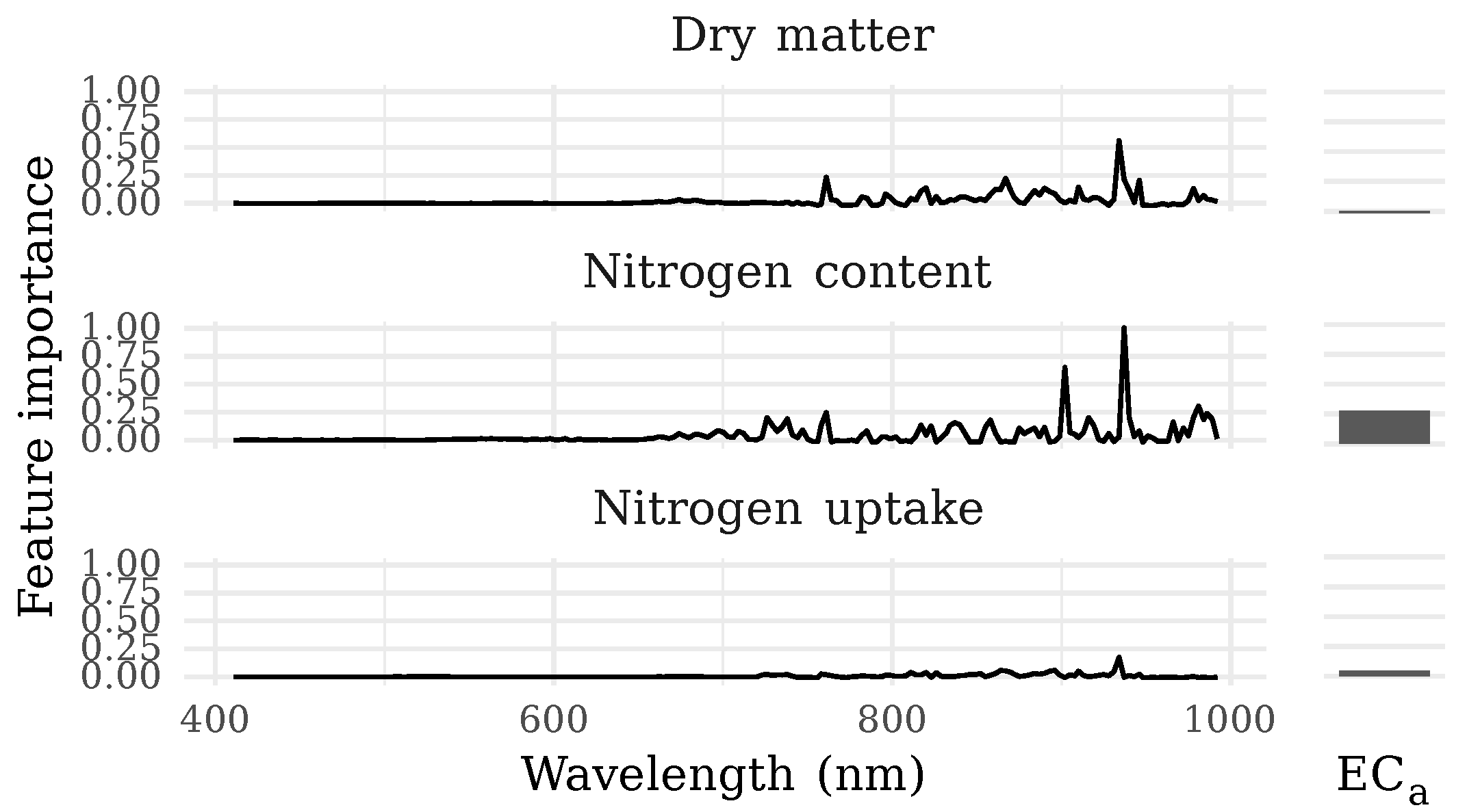
None of the models generated non-physical predictions when applied to whole experimental plots, that is, predictions with negative values or nitrogen content above 100%. The logarithmic transformations removed skew from the values (Figure S2). A similar effect was not observed for the logit transformation because high nitrogen content values were already underrepresented in the dataset. Despite the improved data distributions, a visual comparison of the GPR model validation performance did not signal a systematic influence of the transformations on the model quality (Figure S3). For this reason, we focused on the results pertaining to models trained to the raw crop parameter values, only.
On the contrary, the model predictions differed substantially depending on whether raw or standardized spectra were involved. Although the centering and scaling of the spectra reduced bias for some scenarios, it had a consistent negative effect on the remaining validation metrics, increasing RMSEP and decreasing R 2 and RPD P . Consequently, we proceeded with presenting testing data corresponding to the raw spectra. The interested reader can inspect the results for the omitted scenarios in the Zenodo repository accompanying this article. The predictions clearly differed depending on the choice of imager, the spectra of which were employed for dataset partitioning, albeit not in a systematic way. Therefore, both approaches were included in the more detailed description that follows.

3.2. Dry Matter

The NDRE models predicted dry matter with R 2 of approximately 0.5 or 0.6, depending on dataset partitioning (Table 2). The corresponding RPD P was below 2.0, even in the more favorable scenario, meaning that only qualitative low–high estimates could be expected with the vegetation index [69].
As expected, the predictions obtained with Gaussian process modeling were generally superior to the estimates made with NDRE. However, contrary to our hypothesis, the ESAM models outperformed the SE models only in 3 of the 48 available comparisons across all crop parameters in terms of R 2 , RMSEP , or RPD P . Predicting dry matter with GPR-SE models was associated with improvement in all quality metrics except for bias, where the effect differed across the testing datasets. R 2 was close to 0.75 for the most part, and RPD P above 2.0 could be obtained, with 2.2 as the highest value. At the same time, the models based on the ESAM covariance function often exhibited prediction performance comparable to that of the vegetation index.
The performance of both cameras was similar for GPR-SE models used for dry matter estimation with full-frame camera partitioning (Table 2). For push-broom camera partitioning, the matching camera performed better than the full-frame device, especially in data fusion scenarios. The results were not strongly affected by the augmentation of the spectral dataset with EC a measurements or by the masking of the soil pixels in the imagery. The effect of this latter factor was similarly weak for the other investigated crop parameters.

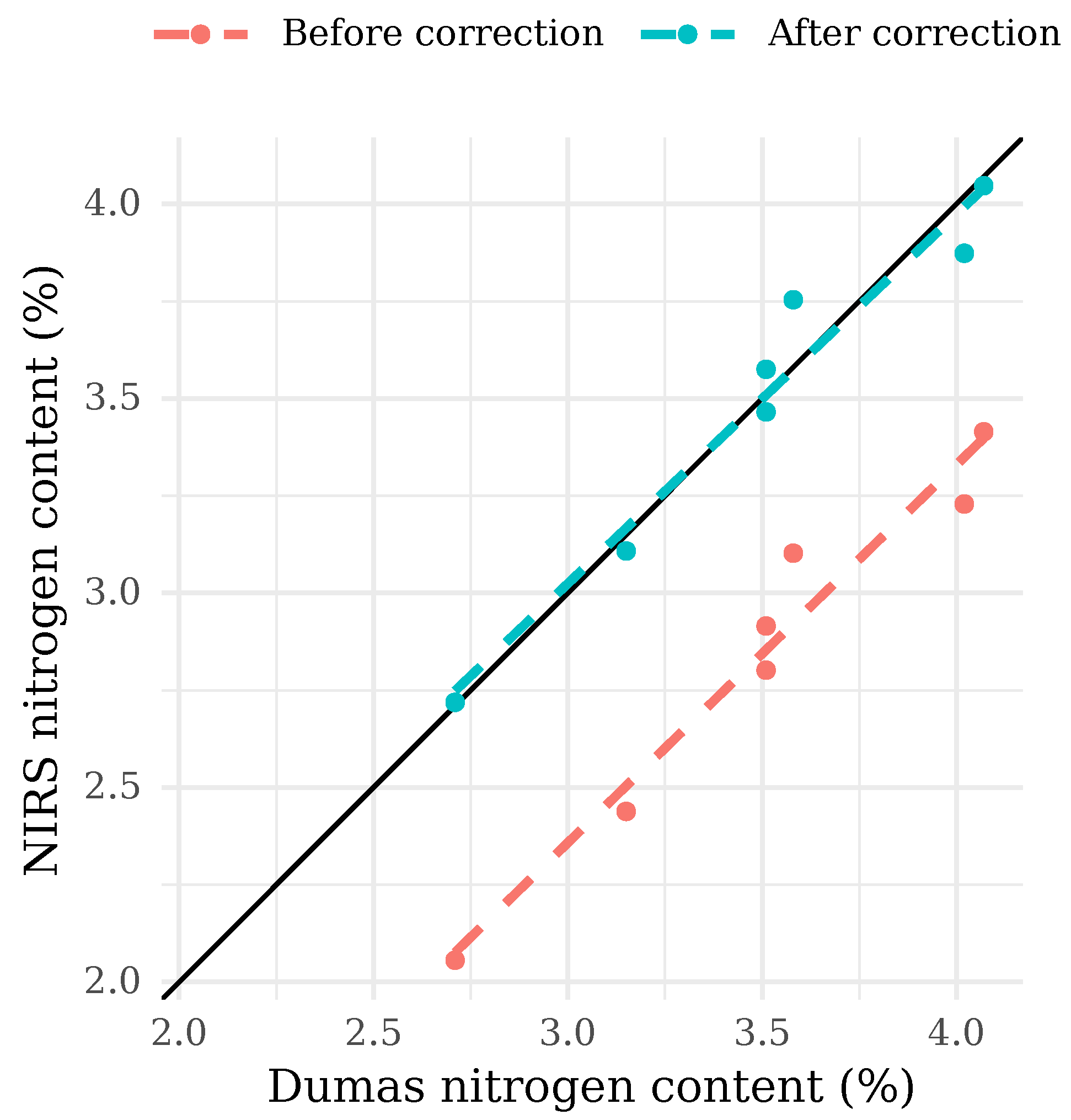
3.3. Nitrogen Content

The vegetation index predicted nitrogen content less accurately than dry matter. Here, the negative R 2 obtained is notable, especially for full-frame camera partitioning (Table 3). An underestimation of the ground truth values could also be noted in the predictions. Among the three investigated crop parameters, nitrogen content prediction quality responded the most strongly to replacing the NDRE index with the GPR models. In particular, the strong negative R 2 values corresponding to dataset partitioning based on full-frame spectra were avoided with GPR-SE models trained using imagery from the same device. However, the negative bias remained in all spectra-only scenarios.
This GPR-SE nitrogen content prediction bias was virtually removed after fusion with EC a measurements. Although the prediction accuracy remained low, for the most part, from the practical point of view, with RPD P below 2.0, the push-broom + EC a predictions corresponding to the push-broom camera dataset partitioning were a notable exception. Here, R 2 exceeded 0.8, and RPD P was close to 2.5, surpassing the result obtained for dry matter (cf. Table 2).

3.4. Nitrogen Uptake

Nitrogen uptake predictions with NDRE were more accurate than for the other crop parameters. R 2 approached 0.8 and RPD P above 2.0 was attained by the ensemble associated with training plots derived from push-broom spectra (Table 4). According to Saeys et al. [69], this was sufficient for applications demanding rough quantitative predictions.
When subjected to GPR-SE modeling, nitrogen uptake was the most accurately predicted property of the three investigated spring wheat parameters. The training of the models to the hyperspectral data alone yielded estimates corresponding to R 2 and RPD P within the 0.75–0.85 and 2.0–2.6 ranges. Similarly to dry matter, GPR’s superiority over NDRE was less clear when the ESAM covariance function was employed.
Augmenting the dataset with EC a measurements improved the GPR-SE model quality, but more important for accurate outcomes was the match between the spectra employed for dataset partitioning and model training. Specifically, the full-frame camera models outperformed those based on push-broom spectra when the dataset partitioning involved full-frame imager data, and vice versa. Combining both effects brought RPD P to the level of 2.7, at which “good” quantitative predictions were possible [69]. The obtained RMSEP of 0.28 and 0.29 g m−2 divided by the testing data ranges [29] of 3.6 and 2.8 g m−2 (Table S1) corresponded to normalized RMSEP ( NRMSEP ) of 7.8 and 10.4%, which was close to the 10% maximum quality threshold adopted by Verrelst et al. [28] and Estévez et al. [29] in their GPR studies.
As a general pattern, regardless of the crop parameter of interest, the highest accuracy was achieved when augmenting the spectra with the EC a measurements and training the GPR model with the SE covariance function to this dataset. The choice of camera appeared to be of minor importance when estimating dry matter and nitrogen uptake, as long as the same imagery was employed for the selection of training samples and training the model. On the other hand, satisfactory nitrogen content predictions could only be obtained with the push-broom imager.

3.5. Evidence of Training Data Overfitting with the ESAM Kernel

In order to more closely examine the negative effect of replacing the SE kernel with ESAM, the model predictions were visualized against the ground truth values for the more challenging full-frame camera partitioning scenarios. For dry matter, the application of the ESAM kernel increased the bias of the estimates obtained with the full-frame imager, as indicated by the direction of the regression lines, while the precision became impaired for the push-broom device, as indicated by the increased scatter of the points around the 1:1 line (left-hand panel in Figure 4). Three isolated points corresponding to high ground truth dry matter were discernible in the plots. These observations exerted high leverage in the NDRE models, biasing their predictions; however, this pattern was absent from the GPR-ESAM models. Instead, their inferiority relative to GPR-SE could be attributed to model overfitting, as indicated by the concentration of the training data points along the 1:1 line, especially for the push-broom camera. A similar pattern was obtained for nitrogen uptake (Figure S4), and the predictions of nitrogen content, especially in the data fusion scenarios, confirmed the GPR-ESAM overfitting problem (right-hand panel in Figure 4). The model validation and testing patterns were similar to those for the NDRE models. However, the high uncertainty values obtained for the estimates correctly signaled that the model outputs should have not been relied upon. This information was not available with the vegetation index.

3.6. Mapping of Crop Parameter Predictions

Figure 5 compares the distribution of crop property ground truth values (first column) with predictions generated by the models associated with the best performance metrics (second column). These were GPR-SE + EC a models trained to push-broom imagery without soil pixel removal. There was a striking agreement between the distribution of low–high predicted values and nitrogen fertilization levels (Figure 1) regardless of the crop property of interest, including those corresponding to the testing experimental plots. Also notable are the high-value plots in the central part of the southern edge, an area associated with high EC a measurements (Figure 1). One of these was included in the biomass collection, and provided the three high-leverage samples that biased the NDRE predictions, as seen in Figure 4, left-hand panel, and Figure S4. Furthermore, dry matter predictions were locally higher in the south-eastern part of the experimental area. This contrasted with the pattern of decreasing nitrogen content along the low-fertilizer experimental plot columns located in the same zone.
Unlike the subplot-level predictions, negative values can be seen in the dry matter and nitrogen uptake maps. These extend along the northern edge, where vehicles were parked and the equipment was placed, including the canvas for UAV take-off and a reflectance panel (Figure 1). However, a single negative pixel can be seen within the field, located in a larger area where the crop was damaged. Low dry matter was predicted in this zone, as well as along the mown strips separating the experimental plots. A similar pattern occurred for nitrogen uptake, whereas the relationship was inverted for nitrogen content, with some of the predicted values considerably exceeding those encountered in the ground truth samples.
The same areas were associated with the highest prediction errors (the third column in Figure 5), being especially apparent for the dry matter and nitrogen uptake models, in the case of which underestimation by more than 50% was frequently signaled. Notably, the plot edges and the damaged experimental plots were also associated with the highest prediction uncertainties (the fourth column). An analogous pattern of overestimation occurred for nitrogen content; however, both the relative error and uncertainty values were more moderate. The individual plot interiors exhibited both positive and negative prediction errors, though not always balanced. The error extremes were more marked in both directions for dry matter and nitrogen uptake than nitrogen content models. Neither error directions nor magnitudes appeared to be systematically affected by plot assignment to the testing data partition. The relative uncertainty was below 10% in much of the area, with higher values, up to 20%, for the low-fertilization plots when predicting dry matter and nitrogen uptake. Similarly to the prediction errors, the uncertainties of the testing plots were comparable to those obtained for the remaining plots.

3.7. Post Hoc Analyses

Permutation feature importance analysis revealed that the predictions primarily involved the NIR spectral region (Figure 6). On the other hand, the visible blue and green reflectance, associated with wavelengths shorter than 550 n m , played little role in obtaining the crop parameter estimates. The pattern corresponding to the dry matter model included five peaks associated with an R 2 drop of more than 0.2 at 761, 867, 934, 937 and 94 n m . Among them, the 934 n m band had a relatively high value of 0.56. The model was not sensitive to EC a measurements. More spectral bands were of high importance when predicting nitrogen content. Two peaks were especially discernible at 902 n m ( R 2 drop of 0.65 upon shuffling) and 937 n m (a drop of 1.00). Also notable are the high value obtained for EC a (0.28), the clear contribution of the red-edge region around 700 n m , and the weak response to the green-red transition bands around 600 n m . The nitrogen uptake model was the least affected by noise in its inputs. The only major peak was at 934 n m , associated with an R 2 drop of 0.17. The sensitivity to the shuffling of EC a was comparable to that estimated for the influential NIR bands.
The analysis of model sensitivity to the choice of NDVI threshold for soil pixel masking revealed the slight impairment of precision and accuracy in terms of R 2 , RMSEP , and RPD P as the threshold value was increased (Table 5). On the other hand, a reduction in bias could be noted for dry matter predictions. The magnitudes of the observed differences were of little practical significance when the scenario without masking was included in the comparison, corroborating the limited influence of soil pixel removal regardless of the threshold.

4. Discussion

4.1. Performance of the Models

We employed the NDRE vegetation index as a benchmark for evaluating the performance of the GPR models. Vegetation indices were originally developed for analyzing multispectral data, and their application in the hyperspectral domain was secondary [70]. Even if scene-specific indices based on lambda–lambda plots are formulated, they exploit the information contained in hyperspectral data cubes only to a limited degree, unlike machine learning methods [20,49]. The fact that the NDRE models were easily biased by high-leverage observations (left-hand panel in Figure 4) and could provide quantitative predictions only of one crop parameter (nitrogen uptake) and in only one dataset partitioning scenario (Table 4) corroborates the limitations of the vegetation index approach.
The GPR-SE models could provide approximate dry matter predictions. Although we do not know of another GPR study aimed at this crop parameter, our results can be contrasted with those devoted to other biophysical quantities. Gewali et al. [12] obtained for the SPARC dataset an R 2 of approximately 0.9 with multiple GPR kernels while predicting LAI and fractional vegetation cover. Verrelst et al. [28] predicted LAI and green LAI (gLAI) with even higher accuracy; however, only cross-validation model performance metrics were reported. None of our models performed so well, and this relative inferiority may be related to a more direct functional relationship that LAI has to VIS-NIR spectra, whereas dry matter and nitrogen content are more indirectly related [71]. The sensitivity of the most accurate dry matter model to the NIR input band information contents (Figure 6) can be related to the influence that vegetation structural parameters have on this spectral region [72].
The GPR models in the present study were unsuitable for applications requiring quantitative nitrogen content when trained only to reflectance spectra. This low performance can be linked to the limited direct relationship of biochemical parameters such as nitrogen in the VIS-NIR spectrum used (400–1000 nm, Table 1). Modeling based on proximal imagery with removed soil pixels enabled the accurate estimates of leaf nitrogen content in the Zhou et al. [14] study with rice. However, the prediction quality deteriorated with decreasing spatial resolution, and R 2 below 0.7 was obtained for ground sample distances above 28 mm px−1, typically encountered in UAV applications. The authors reported an RMSE of more than 0.3%, presumably meaning pp , regardless of the resolution. The R 2 metric of our spectra-only models did not exceed 0.70, either, and although we obtained superior prediction precision, with an RMSEP of 0.20   pp or less regardless of the kernel, this difference can be attributed to the fact that Zhou et al. [14] captured their crop hyperspectral signatures at multiple growth stages. The difficulty of estimating nitrogen content in the present study can be linked to the narrow variation in this parameter relative to other crop characteristics—illustrated by QCV in Table S1—despite varied fertilization levels and the uneven vertical distribution of nitrogen in plants [4]. Wen et al. [33] reported accurate rice nitrogen content predictions with an R 2 of 0.85. However, it is unclear from their study description whether an independent test dataset was employed. A similar issue can be raised for the Zhang et al. [19] publication. Although single vegetation indices selected with the aid of lambda–lambda plots yielded strikingly accurate predictions of the same crop parameter, it is not stated whether the selection was based on training data only, as the data partitions are not referred to until later in the analysis. It would have been beneficial if the authors had published their data and computations to facilitate addressing such questions.
Accurate nitrogen uptake predictions were obtained with GPR-SE. The values of the performance metrics surpassed those obtained for dry matter despite it being hard to estimate nitrogen content in the formulation of the discussed crop parameter. In VIS-NIR plant spectroscopy, the visible spectral region responds primarily to biochemical properties, and the near-infrared region to structural object properties [72]. Perhaps the observed high performance can be linked to an increased amount of spectral information available when a parameter determined by both classes of properties is modeled. Berger et al. [5] predicted nitrogen uptake in winter wheat and corn by combining GPR with radiative transfer modeling. The authors obtained an R 2 of 0.50 and RMSEP of 8.90 g m−2. While their predictions were accurate for low uptake values, an underestimation of the high values was reported. The much superior result obtained in the present study is somewhat surprising given that we employ a less sophisticated analysis workflow. However, it needs to be noted that Berger et al. [5] collected their data at multiple dates, corresponding to a wide range of crop phenological phases. They reported a substantial improvement in predictions when focused only on nitrogen uptake in vegetative parts, with R 2 increasing to 0.86 and RMSEP reduced by a factor of four, which illustrates the influence of the growth stage range. Another hybrid model exhibited better agreement between the predicted and testing data ( R 2 = 0.92 ) than in our study [34]. Although the authors reported a much higher RMSEP of 1.84 g m−2, the difference can, again, be attributed to the higher heterogeneity of observations, which involved two locations and multiple species, including grasses.
The ESAM kernel did not perform as well as the SE kernel in Gaussian process modeling, contrary to the expectation [35], and it was associated with training data overfitting (right-hand panel in Figure 4). Perhaps the advantages of ESAM reveal themselves only in scenes with high illumination variation, including the varied occurrence of shadow pixels and mixed pixels. This possibility is demonstrated by the Gewali et al. [12] simulation, in which SE performance to predict chlorophyll content and fractional vegetation cover deteriorated relative to ESAM model quality as illumination variability increased. Although the light conditions were not stable during the acquisition of our imagery, we only focused on one crop, which might have reduced their negative impact. Moreover, it needs to be noted that even the original proponents of this novel kernel reported mixed results in the context of crop parameter estimation. In the Gewali et al. [12] study, GPR-ESAM outperformed GPR-SE while predicting two biophysical properties, but the R 2 statistics were similar, and RMSE was worse for chlorophyll content in their baseline modeling scenario. At the same time, a pattern of increasing GPR-ESAM superiority relative to GPR-SE was noted when the training sample size was reduced. Our study employs a relatively large training dataset. Verrelst et al. [34] advocated selection of training samples over the maximization of the sample size as a strategy that does not only increase prediction quality, but also reduces the computational complexity of modeling. The latter consideration is especially relevant for GPR, which does not scale well to large datasets [24]. We recommend testing the ESAM kernel with small training datasets in future studies on crop parameter prediction with hyperspectral data.

4.2. The Influence of Training Data Sources

Data fusion can improve predictive model quality by reducing the influence of nuisance parameters on the estimation of the parameter of interest. In the present study, unsatisfactory nitrogen content predictions were obtained with models trained to spectral data alone. Some authors [5,31,73] have highlighted that nitrogen signals are associated primarily with the SWIR region of a reflectance spectrum. Therefore, extending the spectral range to include longer wavelengths might be expected to foster accuracy. Fu et al. [30] augmented RGB color data with texture information and reported a substantial improvement in nitrogen uptake prediction. The recent Zhang et al. [19] study adopted a similar approach with hyperspectral data, also with positive results.
The present study evaluates a fusion between reflectance spectra and EC a . As hypothesized, we obtained evidence of a positive effect not only in relation to nitrogen content prediction quality, but also in the nitrogen uptake models. The latter were the most accurate models obtained in this study, with R 2 above 0.85 and RPD P in the 2.7–2.8 range (Table 4). According to the feature importance analysis, the prediction accuracy of the highest performing nitrogen uptake model was much less affected by the introduction of noise to the input data than when the remaining crop parameters were modeled (Figure 6). The superior performance and robustness can be linked to high within-field soil variability. With the gravitational displacement of clay particles and organic matter observed at the experimental site, the spatial variability of nitrogen sequestration and availability can be expected, which interacted with the effect of varied fertilization rate. In particular, EC a could highlight the fertile area of the field corresponding to the three high-leverage observations in the dataset.
Studies have been published comparing the performance of models trained to VIS-NIR and SWIR or VIS-NIR + SWIR plant imagery [15,74]. Liu et al. [73] examined VIS-NIR predictions of wheat nitrogen content obtained with three hyperspectral sensors operating in proximal mode. However, we did not encounter in the literature a similar VIS-NIR camera comparison that would have involved airborne data. The choice of device had a limited influence while predicting dry matter and nitrogen uptake. However, satisfactory nitrogen content predictions could only be obtained with the push-broom camera, in combination with EC a measurements (Table 3). This pattern can be related to the higher spectral resolution of this imager relative to the full-frame device (Table 1). Narrow bands facilitate the prediction of biochemical parameters [37,70], and crop nitrogen in particular [13]. Accordingly, the model exploited information in the red-edge and visible spectral regions (Figure 6), influenced by chemical vegetation properties [72]. The high importance of the EC a input can be readily linked to the positive effect of data fusion obtained for the discussed crop parameter. The two narrow feature-importance peaks in the NIR corroborate the advantages of a device with a high spectral resolution. Interestingly, the 937 n m or the neighboring 934 n m band were highly influential for estimating each of the three investigated crop properties. Fan et al. [75] noted a correlation between reflectance at the 937 n m first derivative band and corn leaf nitrogen, whereas Yu et al. [76] reported several bands centered slightly below 934 n m as important for estimating total nitrogen content in pepper plants, and related them to carboxylic acid C−H stretch. In the Shorten et al. [77] study, both wavelengths were included in a range determined as especially influential for predicting nitrogen content in ryegrass. The fact that the spectral range of the full-frame camera does not extend beyond 790 n m to capture these features (Table 1) may be another reason why the push-broom device yielded superior nitrogen content predictions.
The removal of soil pixels based on NDVI thresholding was the last factor examined in our study. Its negligible effect can be attributed to the relatively advanced crop growth stage, at which there was a relatively high degree of canopy closure [14], or perhaps, to the inherent flexibility of GPR models, enabling satisfactory predictions even when trained to small and noisy datasets [12,27].

4.3. Prediction Map Patterns

The match between the varied fertilization levels and the obtained spatial distributions of GPR predictions (Figure 5) indicates that the treatments succeeded in generating variation in the crop biophysical parameters in a limited area and that the models are suitable for practical applications. However, even more interesting is the fact that the models were sensitive enough to respond to the natural field variation. The increased dry matter values found in the plants growing in the south-eastern part of the field are likely to be related to soil organic matter accumulation due to erosion processes, while the locally decreased nitrogen content values in the plots corresponding to low fertilization rates can be explained by the dilution effect as the nutrients are distributed over the increased biomass [4]. The fact that the latter pattern is not apparent for the remaining fertilization levels can, in turn, be related to luxury nutrient intake, being able to compensate for the more abundant canopy. It is interesting that neither of the effects prevail in the nitrogen uptake predictions, a parameter that integrates both crop properties. The only notable exceptions are the elevated values corresponding to the plots from which the three high-leverage data points originated. This effect can be explained by the greater variation in dry matter values relative to nitrogen content values in the dataset (Table S1).
The underestimation of pixel values along the mown plot borders demonstrates that the models work as expected, as the ground truth is representative only for the area from where biomass samples were collected, that is, plot interiors. On the other hand, nitrogen content overestimation is somewhat surprising, as lower values would be expected in the exposed lower parts of the canopy [4]. A possible explanation might be the effect of residues that were left after the mowing, perhaps combined with a change in the degree of soil exposure and mechanical crop geometry disturbance affecting its angular reflectance properties. This pattern is similar to the observation of Verrelst et al. [34] of nitrogen detected in fallow fields with crop residues left on the surface. The high prediction uncertainties corresponding to the disturbed plot edges and damaged areas with exposed soil correctly warn the user of the models that the spectral signatures associated with those areas deviate from the calibration domain patterns, and that the outputs should not be relied upon [27]. A similar effect of atypical observations was reported by Verrelst et al. [28]. This valuable information is not available with more mainstream machine learning methods. The within-plot errors are attributable to the different spatial scales of the prediction maps and laboratory samples. The occurrence of both negative and positive error values in the individual plots indicates that the model predictions did not exhibit substantial systematic errors.
Camps-Valls et al. [24] adopted the Global Climate Observing System 20% maximum prediction uncertainty threshold to determine whether estimates are of acceptable quality for practical applications. With the exception of the damaged area, our within-plot predictions fall below this mark, especially the mid- and high-fertilization treatments. The difference in prediction uncertainty between these and the plots that received low nitrogen rates can be linked to higher soil exposure where the canopy was less developed, resulting in mixed pixels with atypical spectral signatures. In favor of this hypothesis is the observation that the uncertainty is low in the south-eastern area, associated with conditions favorable for biomass accumulation. This does not contradict the reported limited effect of soil pixel removal on model performance metrics (Table 2, Table 3 and Table 4), as the model training involved spectra aggregated to the subplot level. The fact that the testing plots are not distinct from the training and validation plots in terms of prediction errors or prediction uncertainties is another sign of satisfactory model quality [24,34]. On the other hand, the obtained predictions with negative values suggest that the application of models trained to ground truth data transformed in a way that avoids such occurrences—log and logit transformations in the present study (Figure S2)—should be reconsidered, even if the effect on overall accuracy is negligible, as shown in Figure S3.

5. Conclusions

The present study demonstrates that a GPR model with the SE covariance function trained to UAV hyperspectral imagery can yield satisfactory estimates of spring wheat biophysical and biochemical parameters after augmentation with proximal EC a measurements. The model quality was significantly higher than the benchmark set by the NDRE vegetation index, with the highest accuracy obtained for nitrogen uptake, which happens to be a key parameter for planning variable nitrogen application. The RPD P was above 2.5, NRMSEP was close to 10 %, and relative estimation uncertainty was below 20%, all indicating the model’s suitability for practical use in precision agriculture. High-quality nitrogen content estimation could only be attained by employing a camera with high spectral resolution and a wide spectral range. The model performance was lower for dry matter, a crop parameter neglected by previous GPR studies. More research is needed to identify possibilities for dry matter prediction improvement. Narrow bands centered at the 934 and 937 n m wavelengths fostered accurate predictions. Substituting SE with the ESAM kernel had a negative effect on prediction quality. We suspect that it may be more suited to scenes with higher heterogeneity than our single-field case, especially when the number of training samples is low. We used historical EC a data, which demonstrates that it is sufficient to collect the measurements for data fusion once and apply them across multiple years, thus avoiding a significant increase in operational costs. The experimental data were collected at the growth stage BBCH39, when the crop can still respond to nitrogen topdressing. This fact further supports the practical applicability of the evaluated modeling approach.

Supplementary Materials

The following supporting information can be downloaded at: https://www.mdpi.com/article/10.3390/rs14235977/s1, Table S1: Descriptive statistics of the collected ground truth data. Each row block corresponds to a crop property, with measurement units given in parentheses. The statistics are presented separately for each data partition. As the partitioning was based on two sets of spectra, yielding different results, each statistic is expressed using two values, and the imager employed for the acquisition of given spectra is indicated. The statistics are based on quartiles because of the deviation of the datasets from a normal distribution; Figure S1: Patterns of apparent soil electrical conductivity measured in the experimental area in 2005 and 2022 after the application of cubic spline interpolation. The 2005 measurements involved SWS–NEN transects with 9–16 m spacing. In 2022, the direction was preserved, while the density was increased by employing more uniform transect spacing of approximately 7 m . EC a —apparent soil electrical conductivity; Figure S2: Left column: Kernel density estimates of the three predicted-variable values. Positive skew is apparent for the dry matter and nitrogen uptake measurements, and a negative skew is discernible for nitrogen content. Right column: The distributions of the same variable values after applying transformations accounting for the physical constraints of the measurements. A logarithm was applied to dry matter and nitrogen uptake, and nitrogen content was subjected to a logit transformation. Units in the parentheses refer to the untransformed values. Although the skew was removed for two parameters, no significant effect on predictive model quality was noted; Figure S3: Influence of data transformations on Gaussian process regression model validation performance. The results are presented separately for data partitioning based on full-frame and push-broom spectra. The boxplot rows correspond to the predicted crop parameters. The columns compare the performance metrics according to whether the ground truth values were transformed prior to the model training. No systematic effect can be discerned here. On the other hand, the misalignments within the individual boxplot pairs signal an influence of spectra standardization. Each boxplot summarizes the quality of the models across scenarios with different combinations of hyperspectral camera, soil pixel removal, and data fusion treatments. The values corresponding to individual performance metrics were centered and scaled to unit variance to account for different numeric ranges. The absolute values were derived for bias prior to the standardization; Figure S4: Nitrogen uptake predictions according to the model and dataset. The individual rows of plots correspond to the three predictive model families either trained to complete hyperspectral imagery or to spectra derived after the removal of soil pixels. The choice of model has a strong effect on the obtained patterns as opposed to the effect of imagery pre-processing. The columns compare the performance of the two hyperspectral cameras. Choosing one over another mostly affects the NDRE predictions. Moreover, the limited effect of data fusion with apparent soil conductivity measurements is depicted. The predictions are displayed relative to the 1:1 line, and those generated from Gaussian process regression models are augmented with error bars corresponding to prediction uncertainty. The patterns are shown separately for the three data partitions employed in modeling. The dashed lines are respective linear regression fits. EC a —apparent soil electrical conductivity; NDRE—normalized difference red edge index model; GPR-SE—Gaussian process regression model with the squared exponential covariance function; GPR-ESAM—Gaussian process regression model with the spectral angle mapper covariance function.

Author Contributions

Conceptualization, W.R.Ż., K.K. and J.G.; Data curation, J.G.; Formal analysis, W.R.Ż. and J.G.; Investigation, W.R.Ż.; Methodology, W.R.Ż., K.K. and J.G.; Resources, J.G.; Visualization, W.R.Ż. and J.G.; Writing—original draft, W.R.Ż.; Writing—review and editing, W.R.Ż., K.K. and J.G. All authors have read and agreed to the published version of the manuscript.

Funding

The work of Wiktor Żelazny was supported by the “Mobility of researchers to support new trends and methods of agricultural research” (“Mobilita vědeckých pracovníků pro podporu nových trendů a zemědělského výzkumu”) project, funded by the Ministry of Education, Youth and Sports of the Czech Republic, grant number CZ.02.2.69/0.0/0.0/18_053/0016953; and by the Ministry of Agriculture of the Czech Republic institutional support, grant number MZE-RO0418. The work of Krzysztof Kusnierek and Jakob Geipel was conducted within the “Innovations for sustainable crop production” (“Innovationer för hållbar växtodling”) project, funded by the EU Interreg ÖKS, grant number 001171. The APC was funded with an MDPI discount voucher.

Institutional Review Board Statement

Not applicable.

Informed Consent Statement

Not applicable.

Data Availability Statement

The pre-processed data are available at Zenodo as part of the doi:10.5281/zenodo.7107300 accession.

Acknowledgments

Field work, UAV mission, and lab analyses were performed with the help of the technical staff at two agricultural research stations, NIBIO-Apelsvoll and NIBIO-Løken. Moreover, the advice of three anonymous reviewers to improve the study and the manuscript is kindly acknowledged.

Conflicts of Interest

We received the Mjolnir data from Norsk Elektro Optikk AS for scientific use, free of charge, without any further conditions/terms or agreements.

References

  1. Späti, K.; Huber, R.; Finger, R. Benefits of Increasing Information Accuracy in Variable Rate Technologies. Ecol. Econ. 2021, 185, 107047. [Google Scholar] [CrossRef]
  2. Poudel, P.B.; Poudel, M.R.; Gautam, A.; Phuyal, S.; Tiwari, C.K.; Bashyal, N.; Bashyal, S. COVID-19 and its Global Impact on Food and Agriculture. J. Biol. Today’s World 2020, 9, 221. [Google Scholar]
  3. Colussi, J.; Schnitkey, G.; Zulauf, C. War in Ukraine and its Effect on Fertilizer Exports to Brazil and the U.S. Farmdoc Dly. 2022, 12, 1–5. [Google Scholar]
  4. Lemaire, G.; Jeuffroy, M.H.; Gastal, F. Diagnosis tool for plant and crop N status in vegetative stage: Theory and practices for crop N management. Eur. J. Agron. 2008, 28, 614–624. [Google Scholar] [CrossRef]
  5. Berger, K.; Verrelst, J.; Féret, J.B.; Hank, T.; Wocher, M.; Mauser, W.; Camps-Valls, G. Retrieval of aboveground crop nitrogen content with a hybrid machine learning method. Int. J. Appl. Earth Obs. Geoinf. 2020, 92, 102174. [Google Scholar] [CrossRef]
  6. Söderström, M.; Piikki, K.; Stenberg, M.; Stadig, H.; Martinsson, J. Producing nitrogen (N) uptake maps in winter wheat by combining proximal crop measurements with Sentinel-2 and DMC satellite images in a decision support system for farmers. Acta Agric. Scand. Sect. B—Soil Plant Sci. 2017, 67, 637–650. [Google Scholar] [CrossRef] [Green Version]
  7. Argento, F.; Anken, T.; Abt, F.; Vogelsanger, E.; Walter, A.; Liebisch, F. Site-specific nitrogen management in winter wheat supported by low-altitude remote sensing and soil data. Precis. Agric. 2021, 22, 364–386. [Google Scholar] [CrossRef]
  8. Stoorvogel, J.J.; Kooistra, L.; Bouma, J. Managing Soil Variability at Different Spatial Scales as a Basis for Precision Agriculture. In Soil-Specific Farming: Precision Agriculture; Advances in Soil Science; Lal, R., Stewart, B., Eds.; CRC Press: Boca Raton, FL, USA, 2015; Volume 22, pp. 37–71. [Google Scholar]
  9. Wójtowicz, M.; Wójtowicz, A.; Piekarczyk, J. Application of remote sensing methods in agriculture. Commun. Biometry Crop. Sci. 2016, 11, 31–50. [Google Scholar]
  10. Banerjee, B.P.; Sharma, V.; Spangenberg, G.; Kant, S. Machine Learning Regression Analysis for Estimation of Crop Emergence Using Multispectral UAV Imagery. Remote Sens. 2021, 13, 2918. [Google Scholar] [CrossRef]
  11. Nex, F.; Armenakis, C.; Cramer, M.; Cucci, D.A.; Gerke, M.; Honkavaara, E.; Kukko, A.; Persello, C.; Skaloud, J. UAV in the advent of the twenties: Where we stand and what is next. ISPRS J. Photogramm. Remote Sens. 2022, 184, 215–242. [Google Scholar] [CrossRef]
  12. Gewali, U.B.; Monteiro, S.T.; Saber, E. Gaussian Processes for Vegetation Parameter Estimation from Hyperspectral Data with Limited Ground Truth. Remote Sens. 2019, 11, 1614. [Google Scholar] [CrossRef] [Green Version]
  13. Fu, Y.; Yang, G.; Pu, R.; Li, Z.; Li, H.; Xu, X.; Song, X.; Yang, X.; Zhao, C. An overview of crop nitrogen status assessment using hyperspectral remote sensing: Current status and perspectives. Eur. J. Agron. 2021, 124, 126241. [Google Scholar] [CrossRef]
  14. Zhou, K.; Cheng, T.; Zhu, Y.; Cao, W.; Ustin, S.L.; Zheng, H.; Yao, X.; Tian, Y. Assessing the Impact of Spatial Resolution on the Estimation of Leaf Nitrogen Concentration Over the Full Season of Paddy Rice Using Near-Surface Imaging Spectroscopy Data. Front. Plant Sci. 2018, 9, 964. [Google Scholar] [CrossRef] [PubMed]
  15. Bruning, B.; Liu, H.; Brien, C.; Berger, B.; Lewis, M.; Garnett, T. The Development of Hyperspectral Distribution Maps to Predict the Content and Distribution of Nitrogen and Water in Wheat (Triticum aestivum). Front. Plant Sci. 2019, 10. [Google Scholar] [CrossRef]
  16. Mao, H.; Meng, J.; Ji, F.; Zhang, Q.; Fang, H. Comparison of Machine Learning Regression Algorithms for Cotton Leaf Area Index Retrieval Using Sentinel-2 Spectral Bands. Appl. Sci. 2019, 9, 1459. [Google Scholar] [CrossRef] [Green Version]
  17. Kganyago, M.; Mhangara, P.; Adjorlolo, C. Estimating Crop Biophysical Parameters Using Machine Learning Algorithms and Sentinel-2 Imagery. Remote Sens. 2021, 13, 4314. [Google Scholar] [CrossRef]
  18. Rosso, P.; Nendel, C.; Gilardi, N.; Udroiu, C.; Chlebowski, F. Processing of remote sensing information to retrieve leaf area index in barley: A comparison of methods. Precis. Agric. 2022, 23, 1449–1472. [Google Scholar] [CrossRef]
  19. Zhang, J.; Cheng, T.; Shi, L.; Wang, W.; Niu, Z.; Guo, W.; Ma, X. Combining spectral and texture features of UAV hyperspectral images for leaf nitrogen content monitoring in winter wheat. Int. J. Remote Sens. 2022, 43, 2335–2356. [Google Scholar] [CrossRef]
  20. Verrelst, J.; Malenovský, Z.; Van der Tol, C.; Camps-Valls, G.; Gastellu-Etchegorry, J.P.; Lewis, P.; North, P.; Moreno, J. Quantifying Vegetation Biophysical Variables from Imaging Spectroscopy Data: A Review on Retrieval Methods. Surv. Geophys. 2019, 40, 589–629. [Google Scholar] [CrossRef] [Green Version]
  21. Martens, H. Reliable and relevant modelling of real world data: A personal account of the development of PLS Regression. Chemom. Intell. Lab. Syst. 2001, 58, 85–95. [Google Scholar] [CrossRef]
  22. Thissen, U.; Pepers, M.; Üstün, B.; Melssen, W.; Buydens, L. Comparing support vector machines to PLS for spectral regression applications. Chemom. Intell. Lab. Syst. 2004, 73, 169–179. [Google Scholar] [CrossRef]
  23. Ziegler, A.; König, I.R. Mining data with random forests: Current options for real-world applications. Wiley Interdiscip. Rev. Data Min. Knowl. Discov. 2014, 4, 55–63. [Google Scholar] [CrossRef]
  24. Camps-Valls, G.; Verrelst, J.; Munoz-Mari, J.; Laparra, V.; Mateo-Jiménez, F.; Gómez-Dans, J. A survey on Gaussian processes for earth-observation data analysis: A comprehensive investigation. IEEE Geosci. Remote Sens. Mag. 2016, 4, 58–78. [Google Scholar] [CrossRef]
  25. Rasmussen, C.E. Gaussian Processes in Machine Learning. In Advanced Lectures on Machine Learning; Lecture Notes in Computer Science; Bousquet, O., von Luxburg, U., Rätsch, G., Eds.; Springer: Berlin/Heidelberg, Germany, 2004; Volume 3176, pp. 63–71. [Google Scholar] [CrossRef] [Green Version]
  26. Schulz, E.; Speekenbrink, M.; Krause, A. A tutorial on Gaussian process regression: Modelling, exploring, and exploiting functions. J. Math. Psychol. 2018, 85, 1–16. [Google Scholar] [CrossRef]
  27. Verrelst, J.; Alonso, L.; Camps-Valls, G.; Delegido, J.; Moreno, J. Retrieval of Vegetation Biophysical Parameters Using Gaussian Process Techniques. IEEE Trans. Geosci. Remote Sens. 2012, 50, 1832–1843. [Google Scholar] [CrossRef]
  28. Verrelst, J.; Rivera, J.P.; Gitelson, A.; Delegido, J.; Moreno, J.; Camps-Valls, G. Spectral band selection for vegetation properties retrieval using Gaussian processes regression. Int. J. Appl. Earth Obs. Geoinf. 2016, 52, 554–567. [Google Scholar] [CrossRef]
  29. Estévez, J.; Berger, K.; Vicent, J.; Rivera-Caicedo, J.P.; Wocher, M.; Verrelst, J. Top-of-Atmosphere Retrieval of Multiple Crop Traits Using Variational Heteroscedastic Gaussian Processes within a Hybrid Workflow. Remote Sens. 2021, 13, 1589. [Google Scholar] [CrossRef]
  30. Fu, Y.; Yang, G.; Li, Z.; Song, X.; Li, Z.; Xu, X.; Wang, P.; Zhao, C. Winter Wheat Nitrogen Status Estimation Using UAV-based RGB Imagery and Gaussian Processes Regression. Remote Sens. 2020, 12, 3778. [Google Scholar] [CrossRef]
  31. Abebe, G.; Tadesse, T.; Gessesse, B. Estimating Leaf Area Index and biomass of sugarcane based on Gaussian process regression using Landsat 8 and Sentinel 1A observations. Int. J. Image Data Fusion 2022, 1–31. [Google Scholar] [CrossRef]
  32. Verrelst, J.; Muñoz, J.; Alonso, L.; Delegido, J.; Rivera, J.P.; Camps-Valls, G.; Moreno, J. Machine learning regression algorithms for biophysical parameter retrieval: Opportunities for Sentinel-2 and -3. Remote Sens. Environ. 2012, 118, 127–139. [Google Scholar] [CrossRef]
  33. Wen, D.; Tongyu, X.; Fenghua, Y.; Chunling, C. Measurement of nitrogen content in rice by inversion of hyperspectral reflectance data from an unmanned aerial vehicle. Ciência Rural 2018, 48, e20180008. [Google Scholar] [CrossRef]
  34. Verrelst, J.; Berger, K.; Rivera-Caicedo, J.P. Intelligent Sampling for Vegetation Nitrogen Mapping Based on Hybrid Machine Learning Algorithms. IEEE Geosci. Remote Sens. Lett. 2020, 18, 2038–2042. [Google Scholar] [CrossRef] [PubMed]
  35. Gewali, U.B.; Monteiro, S.T. A novel covariance function for predicting vegetation biochemistry from hyperspectral imagery with Gaussian processes. In Proceedings of the 2016 IEEE International Conference on Image Processing (ICIP), Phoenix, AZ, USA, 25–28 September 2016; pp. 2216–2220. [Google Scholar] [CrossRef]
  36. Gewali, U.B.; Monteiro, S.T. Spectral angle based unary energy functions for spatial-spectral hyperspectral classification using Markov random fields. In Proceedings of the 2016 8th Workshop on Hyperspectral Image and Signal Processing: Evolution in Remote Sensing (WHISPERS), Los Angeles, CA, USA, 21–24 August 2016; pp. 1–6. [Google Scholar] [CrossRef] [Green Version]
  37. Gewali, U.B.; Monteiro, S.T. A tutorial on modelling and inference in undirected graphical models for hyperspectral image analysis. Int. J. Remote Sens. 2018, 39, 7104–7143. [Google Scholar] [CrossRef] [Green Version]
  38. Heiß, A.; Paraforos, D.S.; Sharipov, G.M.; Griepentrog, H.W. Real-time control for multi-parametric data fusion and dynamic offset optimization in sensor-based variable rate nitrogen application. Comput. Electron. Agric. 2022, 196, 106893. [Google Scholar] [CrossRef]
  39. Crema, A.; Boschetti, M.; Nutini, F.; Cillis, D.; Casa, R. Influence of Soil Properties on Maize and Wheat Nitrogen Status Assessment from Sentinel-2 data. Remote Sens. 2020, 12, 2175. [Google Scholar] [CrossRef]
  40. Wang, W.; Zheng, H.; Wu, Y.; Yao, X.; Zhu, Y.; Cao, W.; Cheng, T. An assessment of background removal approaches for improved estimation of rice leaf nitrogen concentration with unmanned aerial vehicle multispectral imagery at various observation times. Field Crop. Res. 2022, 283, 108543. [Google Scholar] [CrossRef]
  41. Hu, P.; Guo, W.; Chapman, S.C.; Guo, Y.; Zheng, B. Pixel size of aerial imagery constrains the applications of unmanned aerial vehicle in crop breeding. ISPRS J. Photogramm. Remote Sens. 2019, 154, 1–9. [Google Scholar] [CrossRef]
  42. Zhang, J.; Wang, C.; Yang, C.; Xie, T.; Jiang, Z.; Hu, T.; Luo, Z.; Zhou, G.; Xie, J. Assessing the Effect of Real Spatial Resolution of In Situ UAV Multispectral Images on Seedling Rapeseed Growth Monitoring. Remote Sens. 2020, 12, 1207. [Google Scholar] [CrossRef] [Green Version]
  43. Jay, S.; Gorretta, N.; Morel, J.; Maupas, F.; Bendoula, R.; Rabatel, G.; Dutartre, D.; Comar, A.; Baret, F. Estimating leaf chlorophyll content in sugar beet canopies using millimeter-to centimeter-scale reflectance imagery. Remote Sens. Environ. 2017, 198, 173–186. [Google Scholar] [CrossRef]
  44. Heiß, A.; Paraforos, D.S.; Sharipov, G.M.; Griepentrog, H.W. Modeling and simulation of a multi-parametric fuzzy expert system for variable rate nitrogen application. Comput. Electron. Agric. 2021, 182, 106008. [Google Scholar] [CrossRef]
  45. Mouazen, A.; Alhwaimel, S.; Kuang, B.; Waine, T. Fusion of data from multiple soil sensors for the delineation of water holding capacity zones. In Precision Agriculture’13; Stafford, J.V., Ed.; Wageningen Academic Publishers: Lleida, Spain, 2013; pp. 745–751. [Google Scholar]
  46. Ji, W.; Adamchuk, V.I.; Chen, S.; Su, A.S.M.; Ismail, A.; Gan, Q.; Shi, Z.; Biswas, A. Simultaneous measurement of multiple soil properties through proximal sensor data fusion: A case study. Geoderma 2019, 341, 111–128. [Google Scholar] [CrossRef]
  47. Franke, J.; Menz, G. Multi-temporal wheat disease detection by multi-spectral remote sensing. Precis. Agric. 2007, 8, 161–172. [Google Scholar] [CrossRef]
  48. Meier, U. (Ed.) Growth Stages of Mono- and Dicotyledoneous Plants. BBCH Monograph; Federal Biological Research Centre for Agriculture and Forestry: Berlin/Braunschweig, Germany, 2001; p. 158. [Google Scholar]
  49. Geipel, J.; Bakken, A.K.; Jørgensen, M.; Korsaeth, A. Forage yield and quality estimation by means of UAV and hyperspectral imaging. Precis. Agric. 2021, 22, 1437–1463. [Google Scholar] [CrossRef]
  50. Koirala, P.; Løke, T.; Baarstad, I.; Fridman, A.; Hernandez, J. Real-time hyperspectral image processing for UAV applications, using HySpex Mjolnir-1024. In Algorithms and Technologies for Multispectral, Hyperspectral, and Ultraspectral Imagery XXIII; Velez-Reyes, M., Messinger, D.W., Eds.; International Society for Optics and Photonics, SPIE: Anaheim, CA, USA, 2017; Volume 10198, p. 1019807. [Google Scholar] [CrossRef]
  51. Rouse, J.; Hass, R.; Schell, J.; Deering, D. Monitoring vegetation systems in the Great Plains with ERTS. In Third Earth Resources Technology Satellite-1 Symposium; Freden, S.C., Mercanti, E.P., Becker, M.A., Eds.; Goddart Space Flight Center: Washington, DC, USA, 1973; Volume 1, pp. 309–317. [Google Scholar]
  52. Fystro, G.; Lunnan, T. Analysar av grovfôrkvalitet på NIRS. In Plantemøtet Østlandet 2006; Bioforsk FOKUS; Kristoffersen, A.Ø, Ed.; Bioforsk Øst Apelsvoll: Tønsberg, Norway, 2006; Volume 1, pp. 180–181. [Google Scholar]
  53. Jones, D.B. Factors for Converting Percentages of Nitrogen in Foods and Feeds into Percentages of Proteins; US Department of Agriculture Circular: Washington, DC, USA, 1941; pp. 1–22.
  54. Muñoz-Huerta, R.F.; Guevara-Gonzalez, R.G.; Contreras-Medina, L.M.; Torres-Pacheco, I.; Prado-Olivarez, J.; Ocampo-Velazquez, R.V. A Review of Methods for Sensing the Nitrogen Status in Plants: Advantages, Disadvantages and Recent Advances. Sensors 2013, 13, 10823–10843. [Google Scholar] [CrossRef]
  55. Guo, B.B.; Qi, S.L.; Heng, Y.R.; Duan, J.Z.; Zhang, H.Y.; Wu, Y.P.; Feng, W.; Xie, Y.X.; Zhu, Y.J. Remotely assessing leaf N uptake in winter wheat based on canopy hyperspectral red-edge absorption. Eur. J. Agron. 2017, 82, 113–124. [Google Scholar] [CrossRef]
  56. Adamchuk, V.I.; Hummel, J.W.; Morgan, M.T.; Upadhyaya, S.K. On-the-go soil sensors for precision agriculture. Comput. Electron. Agric. 2004, 44, 71–91. [Google Scholar] [CrossRef] [Green Version]
  57. Kennard, R.W.; Stone, L.A. Computer Aided Design of Experiments. Technometrics 1969, 11, 137–148. [Google Scholar] [CrossRef]
  58. Bonfil, D.J.; Michael, Y.; Shiff, S.; Lensky, I.M. Optimizing Top Dressing Nitrogen Fertilization Using VENμS and Sentinel-2 L1 Data. Remote Sens. 2021, 13, 3934. [Google Scholar] [CrossRef]
  59. Kusnierek, K.; Korsaeth, A. Simultaneous identification of spring wheat nitrogen and water status using visible and near infrared spectra and Powered Partial Least Squares Regression. Comput. Electron. Agric. 2015, 117, 200–213. [Google Scholar] [CrossRef]
  60. Song, X.; Xu, D.; Huang, C.; Zhang, K.; Huang, S.; Guo, D.; Zhang, S.; Yue, K.; Guo, T.; Wang, S.; et al. Monitoring of nitrogen accumulation in wheat plants based on hyperspectral data. Remote Sens. Appl. Soc. Environ. 2021, 23, 100598. [Google Scholar] [CrossRef]
  61. Breiman, L. Random Forests. Mach. Learn. 2001, 45, 5–32. [Google Scholar] [CrossRef] [Green Version]
  62. Python Software Foundation. Python Language Reference, Version 3.9. 2021. Available online: https://docs.python.org/3.9/reference/index.html(accessed on 8 August 2022).
  63. Pedregosa, F.; Varoquaux, G.; Gramfort, A.; Michel, V.; Thirion, B.; Grisel, O.; Blondel, M.; Prettenhofer, P.; Weiss, R.; Dubourg, V.; et al. Scikit-learn: Machine Learning in Python. J. Mach. Learn. Res. 2011, 12, 2825–2830. [Google Scholar]
  64. R Core Team. R: A Language and Environment for Statistical Computing; R Foundation for Statistical Computing: Vienna, Austria, 2022. [Google Scholar]
  65. Stevens, A.; Ramirez-Lopez, L.; Hans, G. Prospectr: Miscellaneous Functions for Processing and Sample Selection of Spectroscopic Data, R Package Version 0.2.5. 2022. Available online: https://github.com/l-ramirez-lopez/prospectr(accessed on 18 August 2022).
  66. Byers, J.; Davidson, M.; Zhukov, Y.M. SUNGEO: Sub-National Geospatial Data Archive: Geoprocessing Toolkit; R Package Version 0.2.288; 2022; Available online: https://github.com/zhukovyuri/SUNGEO (accessed on 9 June 2022).
  67. Stallman, R.M.; McGrath, R.; Smith, P.D. GNU Make. A Program for Directing Recompilation; Free Software Foundation: Boston, MA, USA, 2020. [Google Scholar]
  68. Courtès, L.; Wurmus, R. Reproducible and User-Controlled Software Environments in HPC with Guix. In Euro-Par 2015: Parallel Processing Workshops; Hunold, S., Costan, A., Giménez, D., Alexandru, I., Ricci, L., Gómez Requena, M.E., Scarano, V., Verbanescu, A.L., Scott, S.L., Lankes, S., et al., Eds.; Vienna University of Technology: Vienna, Austria, 2015; pp. 579–591. [Google Scholar] [CrossRef] [Green Version]
  69. Saeys, W.; Mouazen, A.M.; Ramon, H. Potential for Onsite and Online Analysis of Pig Manure Using Visible and Near Infrared Reflectance Spectroscopy. Biosyst. Eng. 2005, 91, 393–402. [Google Scholar] [CrossRef]
  70. Mulla, D.J. Twenty five years of remote sensing in precision agriculture: Key advances and remaining knowledge gaps. Biosyst. Eng. 2013, 114, 358–371. [Google Scholar] [CrossRef]
  71. Jones, H.G.; Vaughan, R.A. Integrated applications. In Remote Sensing of Vegetation. Principles, Techniques, and Applications; Oxford University Press: Oxford, UK, 2010; pp. 271–306. [Google Scholar]
  72. Jacquemoud, S.; Ustin, S.L. Leaf optical properties: A state of the art. In Proceedings of the 8th International Symposium of Physical Measurements & Signatures in Remote Sensing, Aussois, France, 8–12 January 2001; pp. 223–332. [Google Scholar]
  73. Liu, H.; Bruning, B.; Garnett, T.; Berger, B. The Performances of Hyperspectral Sensors for Proximal Sensing of Nitrogen Levels in Wheat. Sensors 2020, 20, 4550. [Google Scholar] [CrossRef]
  74. Knauer, U.; Matros, A.; Petrovic, T.; Zanker, T.; Scott, E.S.; Seiffert, U. Improved classification accuracy of powdery mildew infection levels of wine grapes by spatial-spectral analysis of hyperspectral images. Plant Methods 2017, 13, 47. [Google Scholar] [CrossRef] [Green Version]
  75. Fan, L.; Zhao, J.; Xu, X.; Liang, D.; Yang, G.; Feng, H.; Yang, H.; Wang, Y.; Chen, G.; Wei, P. Hyperspectral-Based Estimation of Leaf Nitrogen Content in Corn Using Optimal Selection of Multiple Spectral Variables. Sensors 2019, 19, 2898. [Google Scholar] [CrossRef] [Green Version]
  76. Yu, K.Q.; Zhao, Y.R.; Li, X.L.; Shao, Y.N.; Liu, F.; He, Y. Hyperspectral Imaging for Mapping of Total Nitrogen Spatial Distribution in Pepper Plant. PLoS ONE 2014, 9, e116205. [Google Scholar] [CrossRef]
  77. Shorten, P.R.; Leath, S.R.; Schmidt, J.; Ghamkhar, K. Predicting the quality of ryegrass using hyperspectral imaging. Plant Methods 2019, 15, 63. [Google Scholar] [CrossRef]
Figure 1. Layout of the experiment depicting fertilization levels, varied across the plot columns to obtain a dataset with wide ranges of biophysical and biochemical crop parameter values. The numbers indicate distinct plot pairs, and the rows of plots from which biomass samples were collected are indicated. The three passes of the grass harvester along each of the rows are also marked. Apparent soil electrical conductivity measurements are displayed in m S   m 1 using isolines. The coordinates are in the system described by the EPSG:25832 code.
Remotesensing 14 05977 g001
Figure 2. Walter and Lieth diagram of weather conditions in the year of the experiment. The red and blue lines depict mean temperatures and precipitation sums, and red and blue areas correspond to dry and humid periods. The values on the left are temperature extremes for the whole year, and the boxes along the abscissa mark months with frost risk. Note the period of drought signaled in May, when the crop was sown. Source: Agrometeorology Norway (https://lmt.nibio.no, accessed on 25 August 2022).
Remotesensing 14 05977 g002
Figure 3. Accuracy validation of nitrogen content ground truth estimates obtained using laboratory near-infrared spectroscopy. The estimated values (the ordinate axis) are compared with Dumas nitrogen content values (the abscissa). The negative bias of approximately 0.75   pp relative to the 1:1 line, marked in black, is discernible. Ground truth with the bias removed, which is used in subsequent modeling, is also depicted. The dashed lines correspond to linear regression fits before and after the correction.
Remotesensing 14 05977 g003
Figure 4. Dry matter and nitrogen content predictions according to the model and dataset. The individual rows of plots correspond to the three predictive model families either trained to complete hyperspectral imagery or to spectra derived after the removal of soil pixels. The choice of model has a strong effect on the obtained patterns as opposed to the effect of imagery pre-processing. The columns within each of the two panels compare the performance of the two hyperspectral cameras. Choosing one over another mostly affects the NDRE predictions. Moreover, the limited effect of data fusion with apparent soil electrical conductivity measurements is depicted. The predictions are displayed relative to the 1:1 line, and those generated from Gaussian process regression models are augmented with error bars corresponding to prediction uncertainty. The patterns are shown separately for the three data partitions employed in modeling. The dashed lines are the respective linear regression fits. EC a —apparent soil electrical conductivity, NDRE—normalized difference red edge index model, GPR-SE—Gaussian process regression model with the squared exponential covariance function, GPR-ESAM—Gaussian process regression model with the spectral angle mapper covariance function.
Remotesensing 14 05977 g004
Figure 5. Ground truth (first column), prediction (second column), relative prediction error (third column), and relative prediction uncertainty (fourth column) maps for individual crop properties. A relative error of 1 corresponds to no prediction error. The value estimates were generated using the highest-performing models. These were Gaussian process regression models with the squared exponential kernel trained to raw push-broom hyperspectral reflectance data augmented with apparent soil electrical conductivity measurements. The predicted crop property is indicated above each row. Values are not available for the easternmost experimental plot column, which was not covered by the push-broom imagery. The color scale upper cutoffs for the predictions are 120% of the highest ground truth values, and negative predictions are not shown. The displayed errors are trimmed at ±50%, and the uncertainty values at 50%. The biomass collection strips corresponding to the testing data partition are marked with black frames.
Remotesensing 14 05977 g005
Figure 6. Permutation importance of input features corresponding to the highest-performing models. These were Gaussian process regression models with the squared exponential kernel trained to raw push-broom hyperspectral reflectance data augmented with apparent soil electrical conductivity measurements. The predicted crop property is indicated above each row. The feature importance is given on the R 2 scale. EC a —apparent soil electrical conductivity.
Remotesensing 14 05977 g006
Table 1. Technical specification and setup of the hyperspectral cameras employed in the study.
Rikola HSIMjolnir V-1240
sensing typefull-framepush-broom
spectral discriminationFabry–Pérot interferometerdispersion grating
image sensorCMOSNA
field of view (°)36.520
F-number2.81.8
focal length ( m m )9NA
image dimensions ( px )1010 × 10101240
ground sample distance ( c m )44
band count29200
spectral range ( n m )460–790400–1000
spectral step ( n m )5–203
full width at half maximum ( n m )9.85–19.352
radiometric resolution ( bit )1212
NA—information unavailable.
Table 2. Dry matter prediction performance metrics of individual model families across the testing datasets according to the device which provided spectra for dataset partitioning and for model training. The four column blocks examine the effects of removing soil pixels from the hyperspectral imagery prior to model training or augmenting the spectral data with measurements of apparent soil electrical conductivity. The three row blocks correspond to the predicted variables. The values of bias and RMSEP are in g m 2 . The individual rows of each block compare the performance of the cameras and predictive model formulations. The results with the best metrics for each training dataset are marked in bold.
Partitioning
Imager
Modeling
Imager
SpectraSpectra, Soil Pixels RemovedSpectra + EC a Spectra + EC a , Soil Pixels Removed
R2BiasRMSEPRPDpR2BiasRMSEPRPDpR2BiasRMSEPRPDpR2BiasRMSEPRPDp
NDRE
full-framefull-frame0.620.6121.640.610.3131.610.630.9121.680.630.7121.66
push-broom0.560.5131.520.530.1141.480.560.6131.530.540.4131.50
push-broomfull-frame0.524.5131.470.514.2131.450.544.9131.490.534.7131.47
push-broom0.506.0131.430.466.0141.370.506.3131.430.456.3141.37
GPR-SE
full-framefull-frame0.77−2.3102.100.76−2.7102.050.77−0.5102.100.76−0.7102.06
push-broom0.77−3.0102.100.75−3.4102.050.75−3.3102.030.75−3.2102.01
push-broomfull-frame0.730.4101.950.740.191.990.661.0111.740.630.5111.67
push-broom0.790.892.200.770.692.110.791.292.190.770.892.10
GPR-ESAM
full-framefull-frame0.600.0131.610.63−0.1121.670.660.4121.730.640.4121.69
push-broom0.65−2.2121.710.66−2.1121.740.66−0.7121.750.60−0.2131.61
push-broomfull-frame0.77−1.692.100.73−1.6101.940.501.7131.440.481.5131.40
push-broom0.751.792.010.722.9101.910.553.9121.510.464.0141.38
ECa—apparent soil electrical conductivity, R2—coefficient of determination, RMSEP—root mean squared error of prediction, RPDP—ratio of prediction to deviation of prediction, NDRE—normalized difference red edge index model, GPR-SE—Gaussian process regression model with the squared exponential covariance function, GPR-ESAM—Gaussian process regression model with the spectral angle mapper covariance function.
Table 3. Nitrogen content prediction performance metrics of individual model families across the testing datasets according to the device which provided spectra for dataset partitioning and for model training. The four column blocks examine the effects of removing soil pixels from the hyperspectral imagery prior to model training or augmenting the spectral data with measurements of apparent soil electrical conductivity. The three row blocks correspond to the predicted variables. The values of bias and RMSEP are in pp. The individual rows of each block compare the performance of the cameras and predictive model formulations. The results with the best metrics for each training dataset are marked in bold.
Partitioning
Imager
Modeling
Imager
SpectraSpectra, Soil Pixels RemovedSpectra + EC a Spectra + EC a , Soil Pixels Removed
R2BiasRMSEPRPDpR2BiasRMSEPRPDpR2BiasRMSEPRPDpR2BiasRMSEPRPDp
NDRE
full-framefull-frame−0.79−0.130.240.76−0.81−0.130.240.75−0.75−0.120.240.77−0.77−0.120.240.76
push-broom−0.64−0.130.230.79−0.63−0.130.230.79−0.60−0.120.230.80−0.57−0.120.220.81
push-broomfull-frame−0.07−0.150.250.98−0.07−0.150.250.98−0.06−0.150.250.99−0.06−0.150.250.98
push-broom0.04−0.130.241.030.07−0.130.231.050.04−0.130.241.040.08−0.130.231.06
GPR-SE
full-framefull-frame0.40−0.070.141.310.50−0.060.131.440.350.000.141.260.360.020.141.26
push-broom−0.08−0.110.190.97−0.10−0.110.190.970.38−0.010.141.290.37−0.010.141.28
push-broomfull-frame0.66−0.050.141.750.68−0.050.141.790.72−0.030.131.910.70−0.020.131.84
push-broom0.69−0.060.131.830.67−0.060.141.780.83−0.020.102.450.82−0.020.102.41
GPR-ESAM
full-framefull-frame−0.20−0.090.200.92−0.19−0.090.200.93−0.27−0.100.200.90−0.30−0.100.200.89
push-broom0.11−0.080.171.070.19−0.070.161.13−0.37−0.130.210.87−0.36−0.130.210.87
push-broomfull-frame0.44−0.080.181.360.48−0.070.171.410.58−0.080.161.570.59−0.090.151.58
push-broom0.61−0.080.151.620.65−0.080.141.720.35−0.110.191.250.39−0.100.191.30
ECa—apparent soil electrical conductivity, R2—coefficient of determination, RMSEP—root mean squared error of prediction, RPDP—ratio of prediction to deviation of prediction, NDRE—normalized difference red edge index model, GPR-SE—Gaussian process regression model with the squared exponential covariance function, GPR-ESAM—Gaussian process regression model with the spectral angle mapper covariance function.
Table 4. Nitrogen uptake prediction performance metrics of individual model families across the testing datasets according to the device which provided spectra for dataset partitioning and for model training. The four column blocks examine the effects of removing soil pixels from the hyperspectral imagery prior to model training or augmenting the spectral data with measurements of apparent soil electrical conductivity. The three row blocks correspond to the predicted variables. The values of bias and RMSEP are in g m 2 . The individual rows of each block compare the performance of the cameras and predictive model formulations. The results with the best metrics for each training dataset are marked in bold.
Partitioning
Imager
Modeling
Imager
SpectraSpectra, Soil Pixels RemovedSpectra + EC a Spectra + EC a , Soil Pixels Removed
R2BiasRMSEPRPDpR2BiasRMSEPRPDpR2BiasRMSEPRPDpR2BiasRMSEPRPDp
NDRE
full-framefull-frame0.69−0.110.431.810.67−0.120.441.770.72−0.090.411.900.71−0.100.421.88
push-broom0.66−0.110.451.750.64−0.120.471.690.68−0.100.441.790.67−0.110.451.76
push-broomfull-frame0.760.000.392.070.75−0.010.402.020.780.020.382.160.770.010.392.10
push-broom0.800.080.362.250.770.080.392.110.800.090.362.270.770.090.382.11
GPR-SE
full-framefull-frame0.81−0.150.342.320.81−0.150.342.320.87−0.060.282.780.86−0.060.292.72
push-broom0.76−0.200.382.060.75−0.210.392.040.83−0.120.322.470.83−0.130.322.46
push-broomfull-frame0.82−0.030.342.420.83−0.040.332.440.83−0.010.332.470.83−0.020.332.43
push-broom0.84−0.050.322.570.84−0.050.332.500.870.020.292.770.860.020.302.70
GPR-ESAM
full-framefull-frame0.66−0.110.451.740.68−0.110.441.790.74−0.130.392.000.74−0.130.401.98
push-broom0.67−0.180.441.770.67−0.170.451.760.70−0.200.431.840.69−0.170.431.81
push-broomfull-frame0.74−0.130.402.000.74−0.150.402.010.68−0.080.451.800.68−0.080.461.78
push-broom0.81−0.040.352.330.800.010.362.280.730.010.411.960.690.020.441.83
ECa—apparent soil electrical conductivity, R2—coefficient of determination, RMSEP—root mean squared error of prediction, RPDP—ratio of prediction to deviation of prediction, NDRE—normalized difference red edge index model, GPR-SE—Gaussian process regression model with the squared exponential covariance function, GPR-ESAM—Gaussian process regression model with the spectral angle mapper covariance function.
Table 5. Sensitivity of model prediction quality to the choice of soil–vegetation pixel segmentation threshold. Metrics of the most accurate models are presented. These were Gaussian process regression models with the squared exponential kernel trained to raw push-broom hyperspectral reflectance data augmented with apparent soil electrical conductivity measurements. Groups of the columns correspond to the individual estimated crop parameters. The units of bias and RMSEP values are given in parentheses. The rows compare the model performances.
NDVI
Threshold
Dry Matter ( g   m 2 )Nitrogen Content ( pp )Nitrogen Uptake ( g   m 2 )
R2BiasRMSEPRPDpR2BiasRMSEPRPDpR2BiasRMSEPRPDp
No segmentation0.791.28.62.190.83−0.0200.102.450.870.0200.292.77
0.300.781.08.62.190.83−0.0200.102.440.870.0200.292.76
0.350.780.88.62.180.83−0.0200.102.430.860.0200.292.76
0.400.780.88.72.160.83−0.0200.102.420.860.0200.302.75
0.450.770.88.82.130.82−0.0200.102.410.860.0200.302.73
0.500.770.88.92.100.82-0.0200.102.410.860.0200.302.70
NDVI—normalized difference vegetation index, R2—coefficient of determination, RMSEP—root mean squared error of prediction, RPDP—ratio of prediction to deviation of prediction.
Publisher’s Note: MDPI stays neutral with regard to jurisdictional claims in published maps and institutional affiliations.

