
A Framework for Distributed LEO SAR Air Moving Target 3D Imaging via Spectral Estimation

Abstract
1. Introduction
2. Preliminaries and Methods
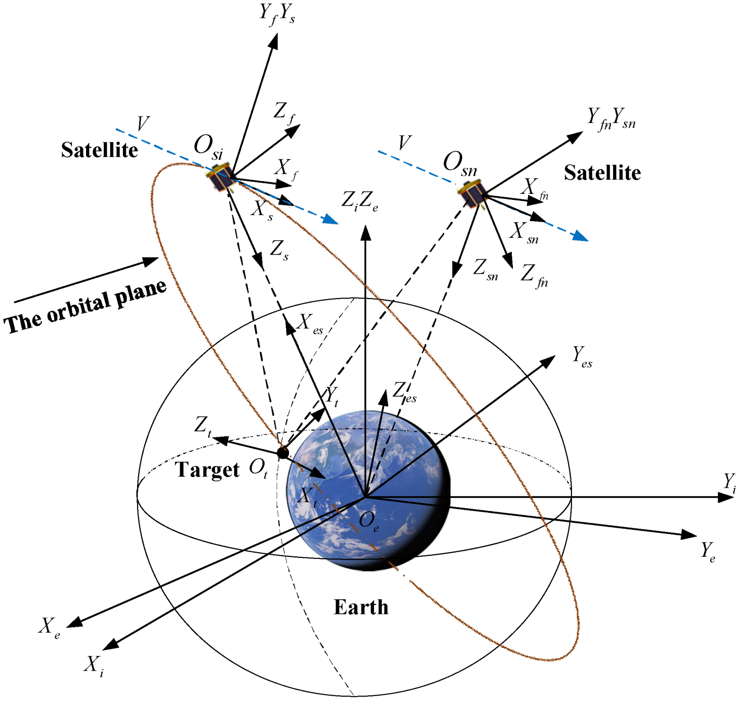
2.1. Coordinate System
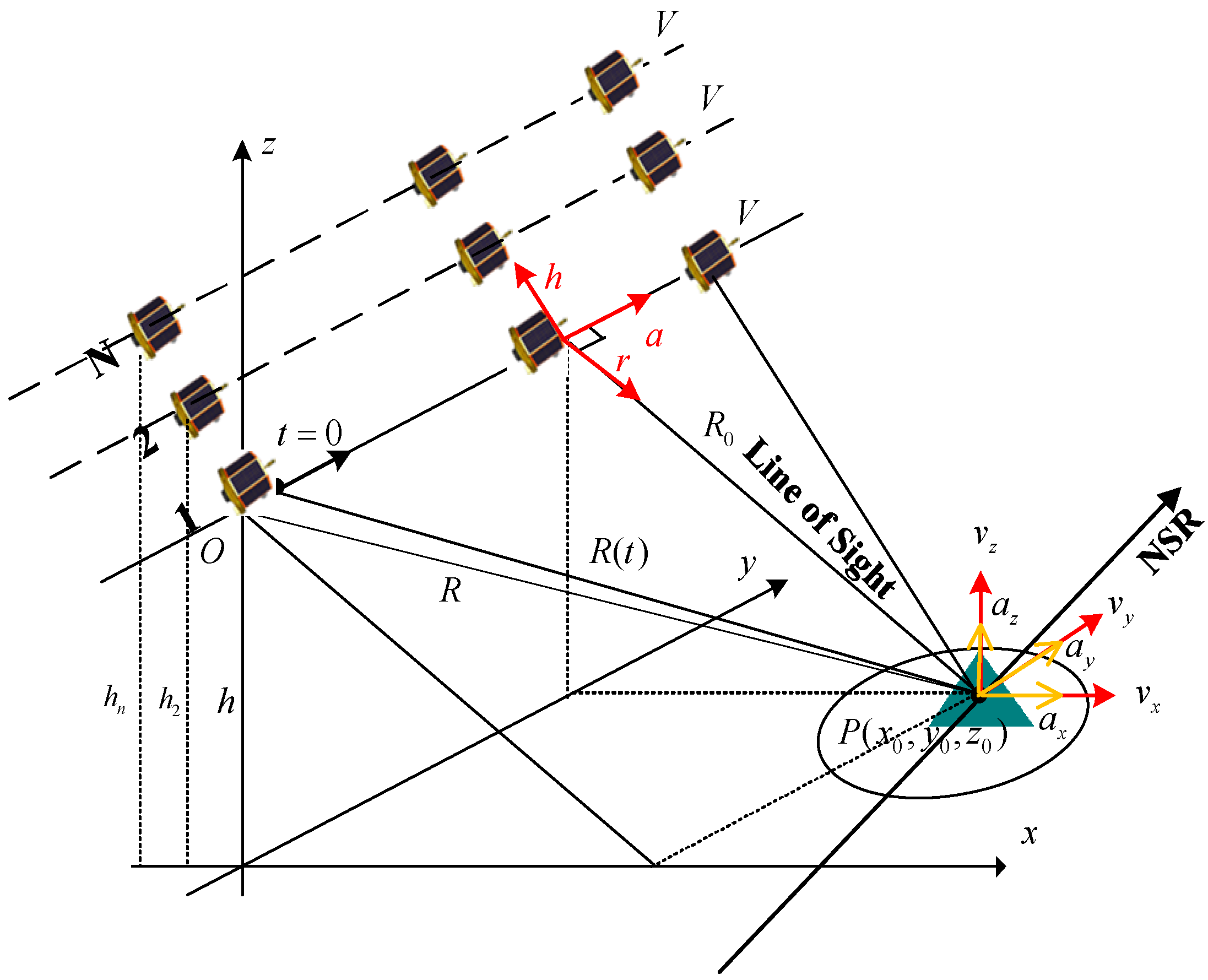
2.2. Model of 3D SAR Moving Target Imaging
2.3. SAR Moving Target 3D Imaging Performance Analysis
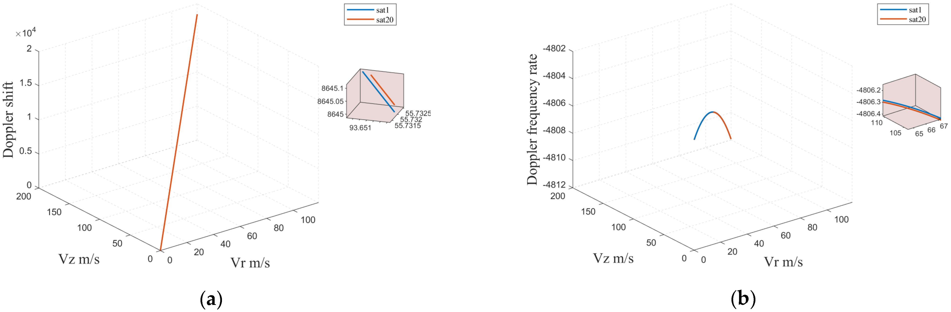
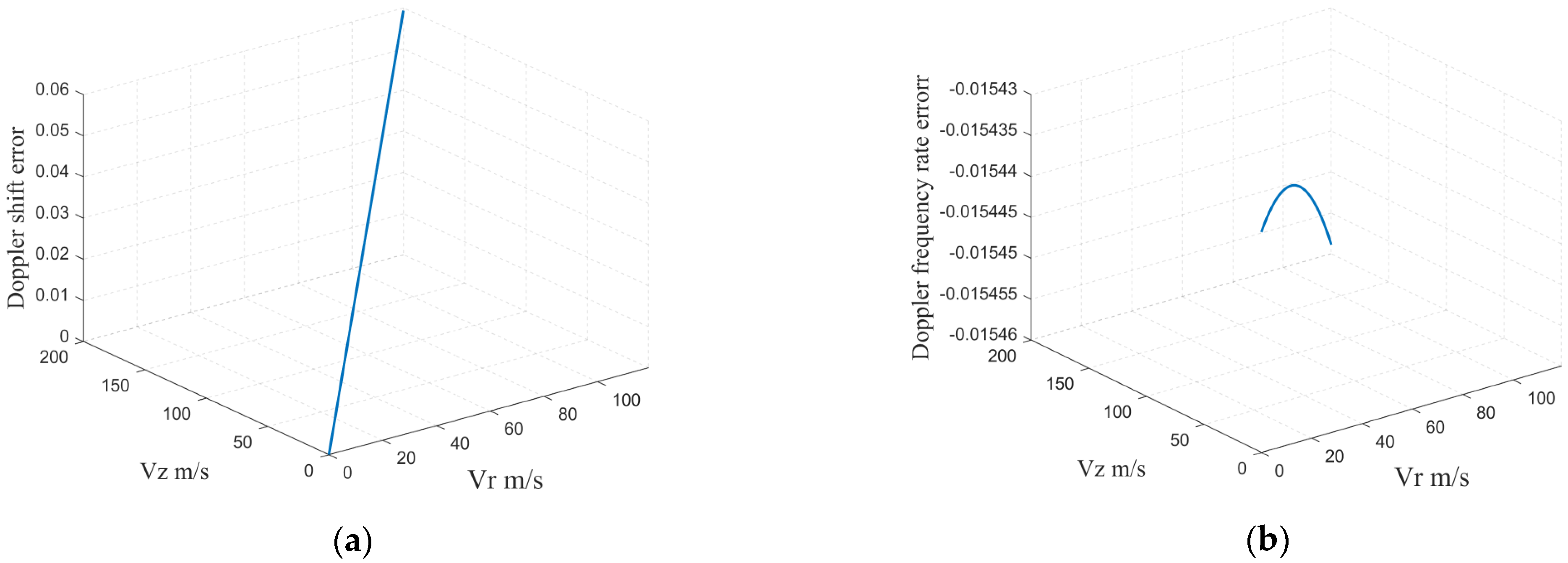
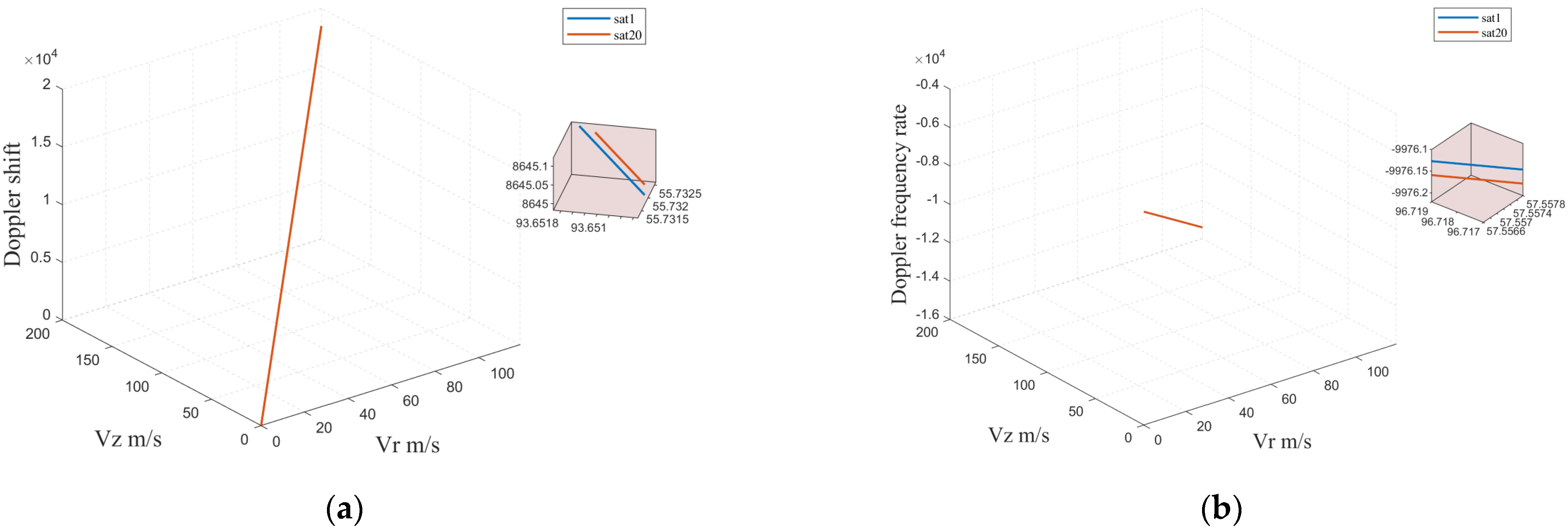
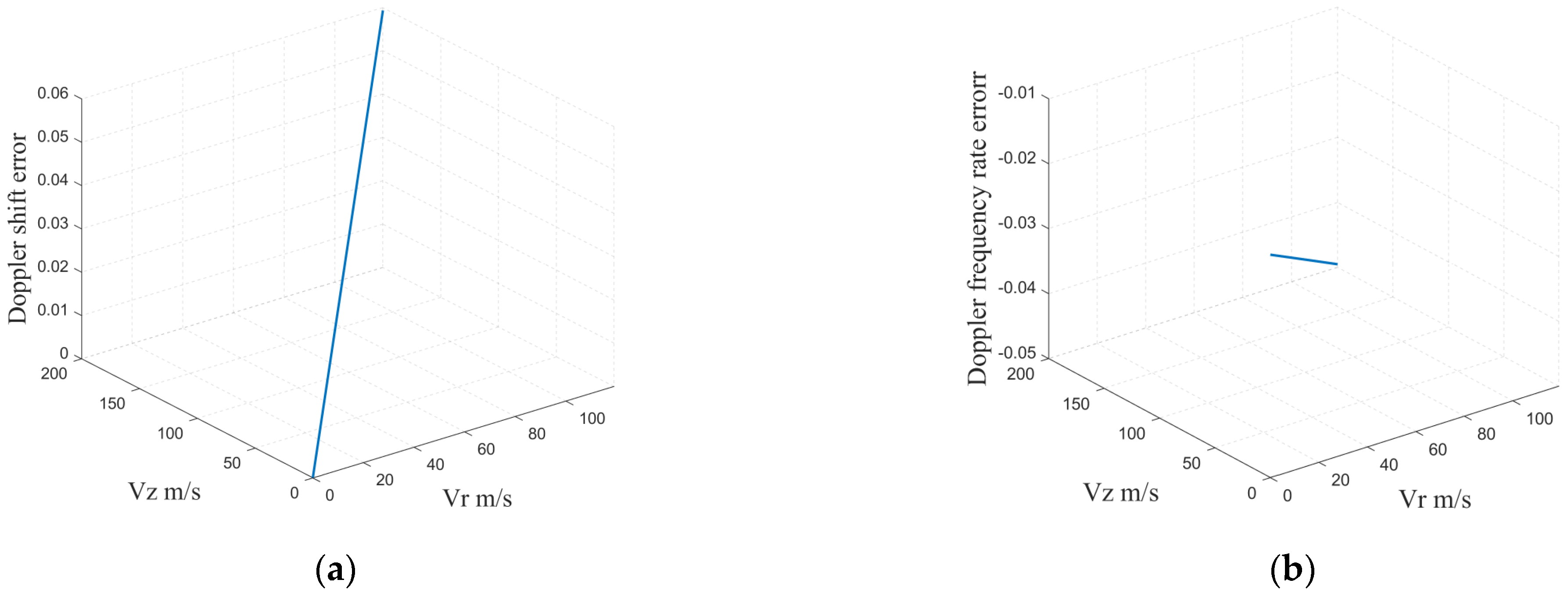
2.3.1. Doppler Performance with Velocity and Acceleration
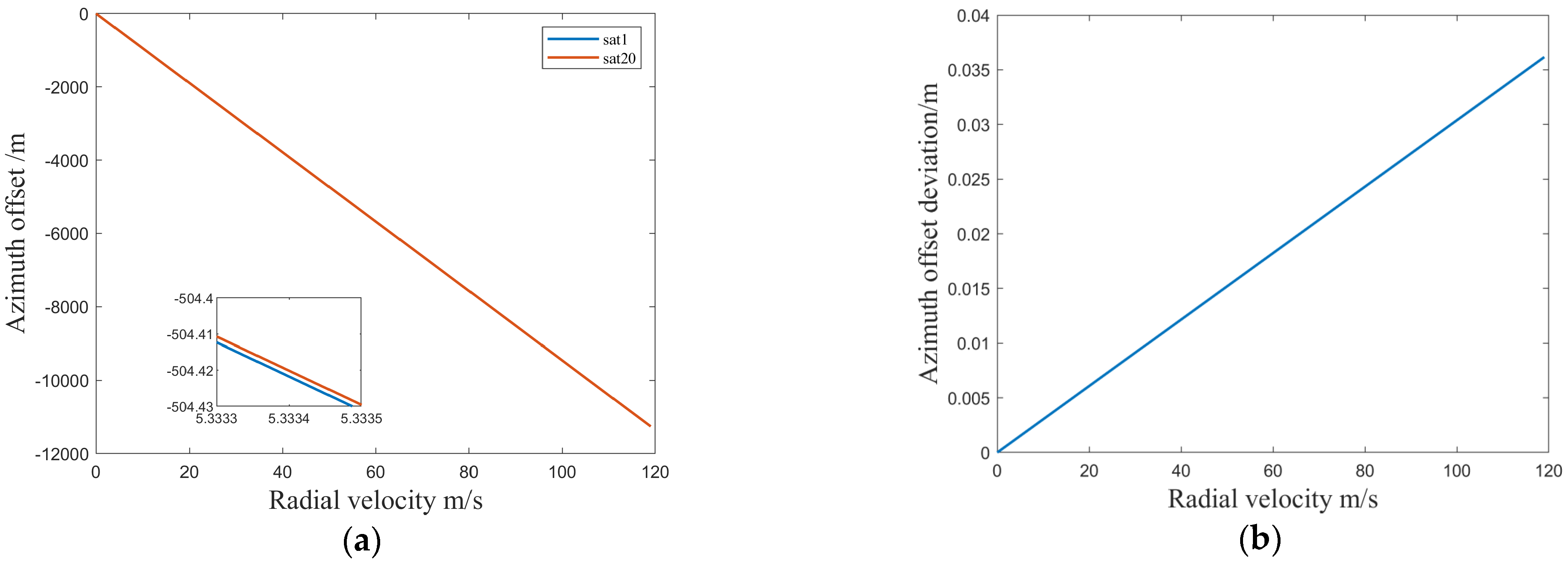
2.3.2. Azimuth Offset
2.3.3. RVP Phase
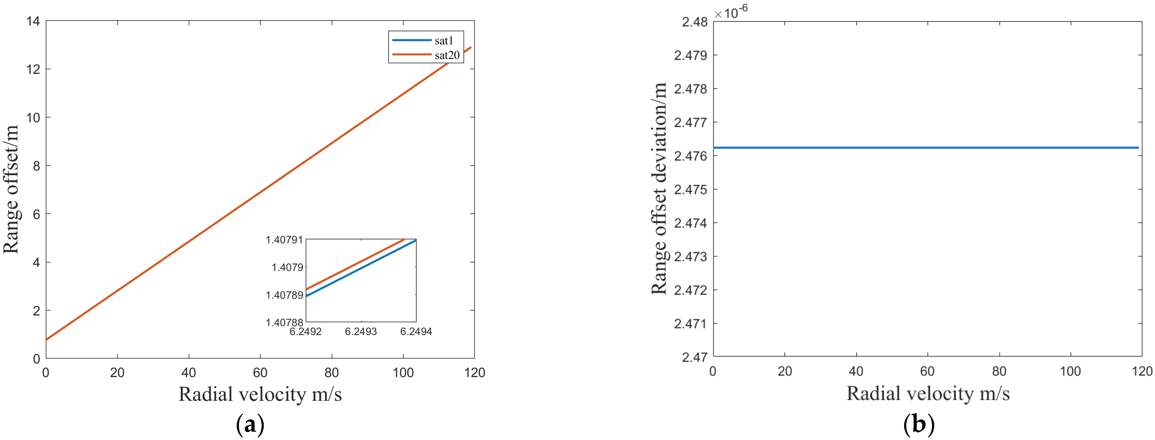
2.3.4. Azimuth Defocus and Range Contamination
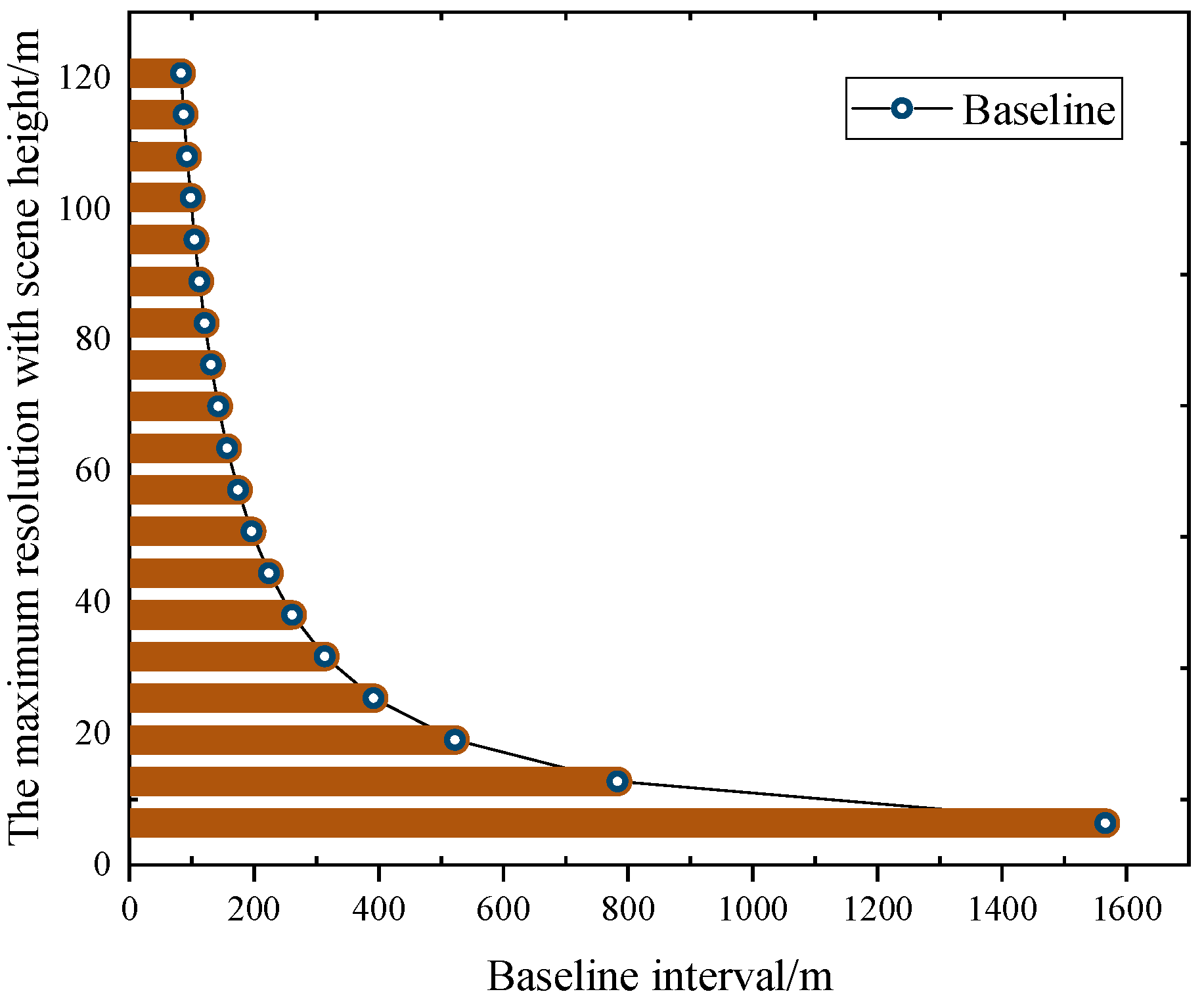
2.3.5. Baseline Interval
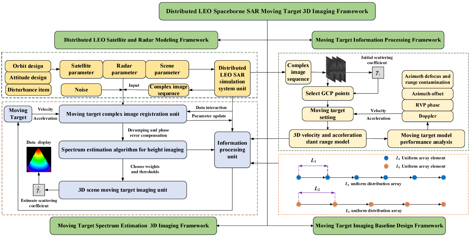
2.4. Distributed LEO Spaceborne SAR Moving Target 3D Imaging Framework
2.5. Method of the Distributed LEO Spaceborne SAR Moving Target 3D Imaging
2.5.1. Beamforming for 3D Moving Target
2.5.2. Capon for 3D Moving Target
2.5.3. MUSIC for 3D Moving Target
3. Simulation Results
3.1. Simulation Parameters
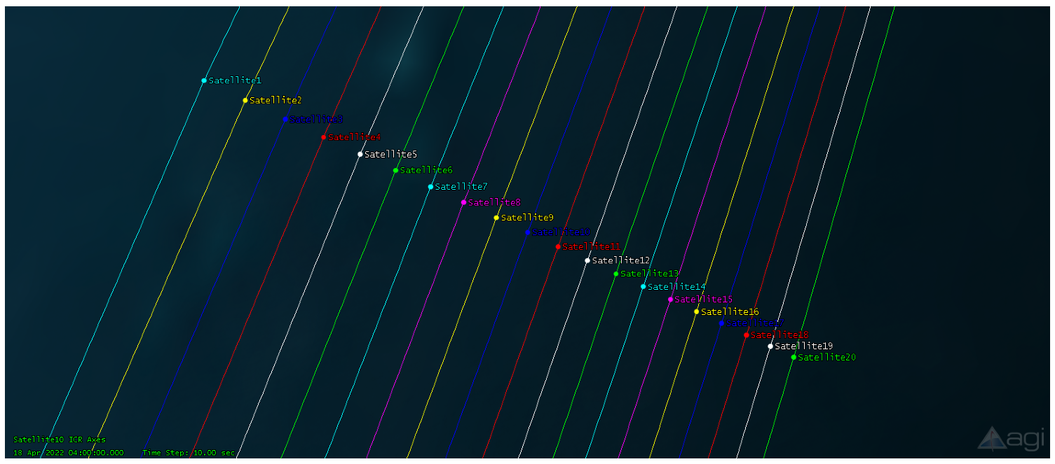
3.1.1. Satellite Parameters
3.1.2. Radar Parameters
3.2. Simulation Results
3.2.1. SAR Moving Target 3D Imaging Performance Analysis
- Case 1: Doppler Performance with velocity and acceleration
- Case 2: Azimuth Offset
- Case 3: Baseline Interval
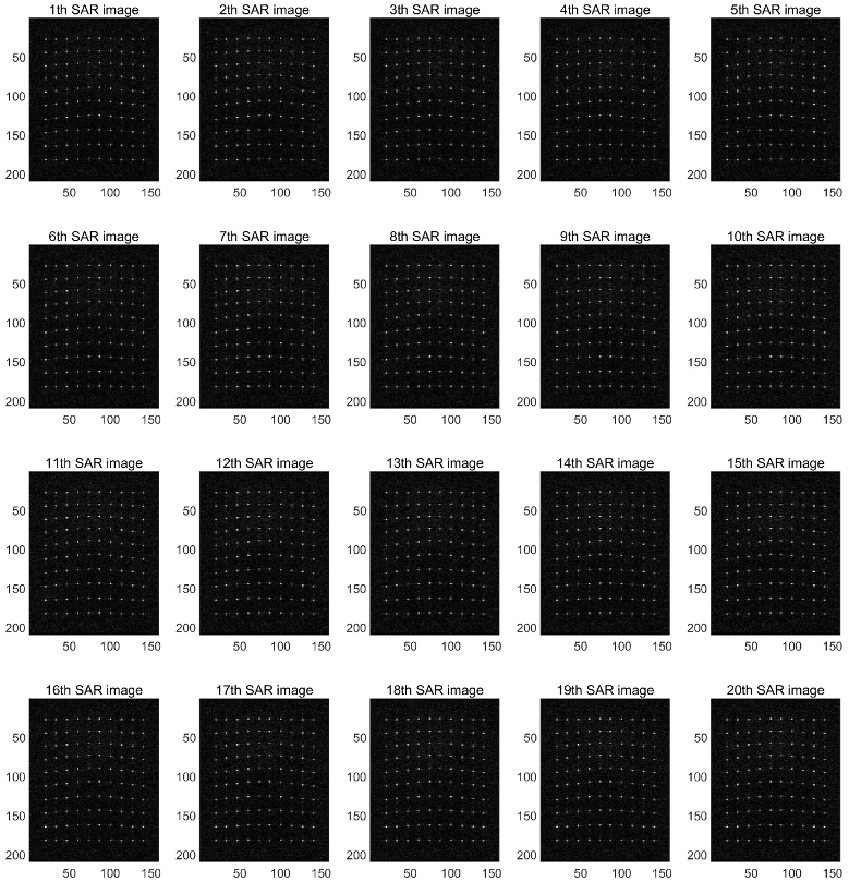
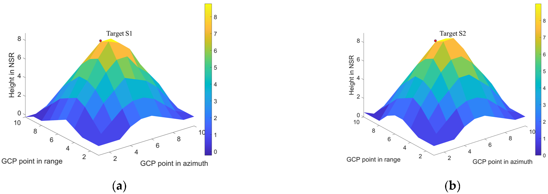
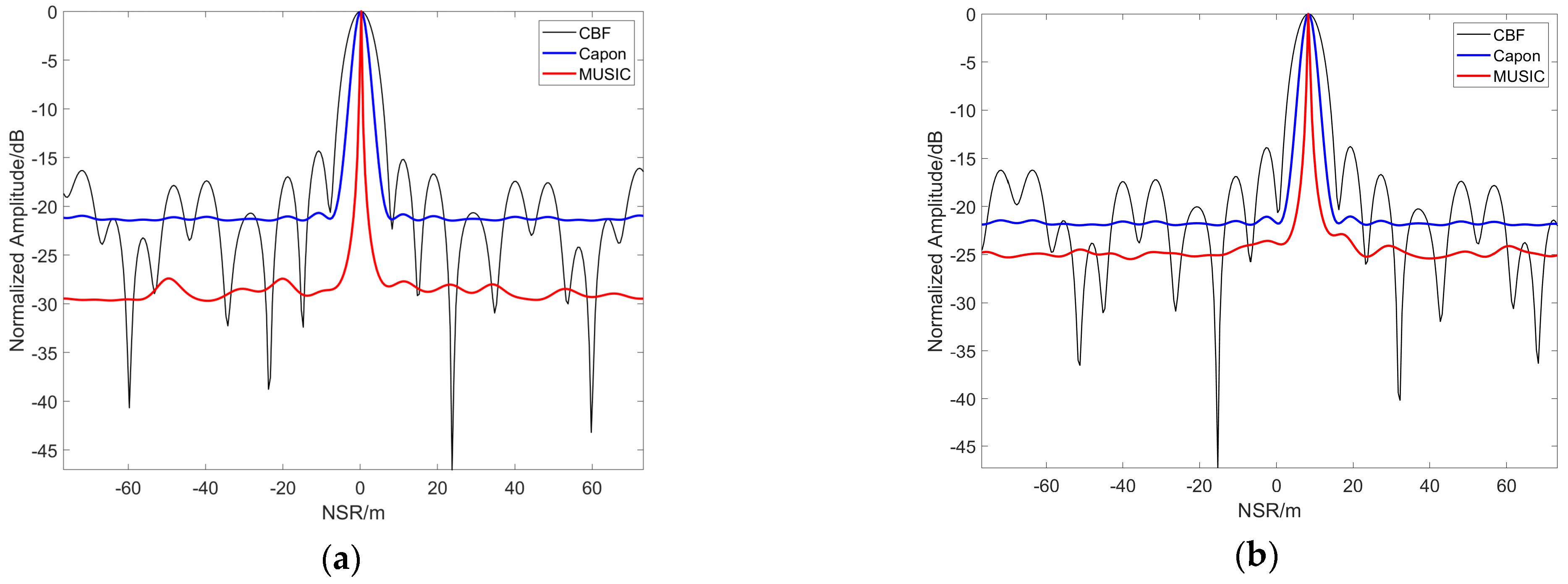
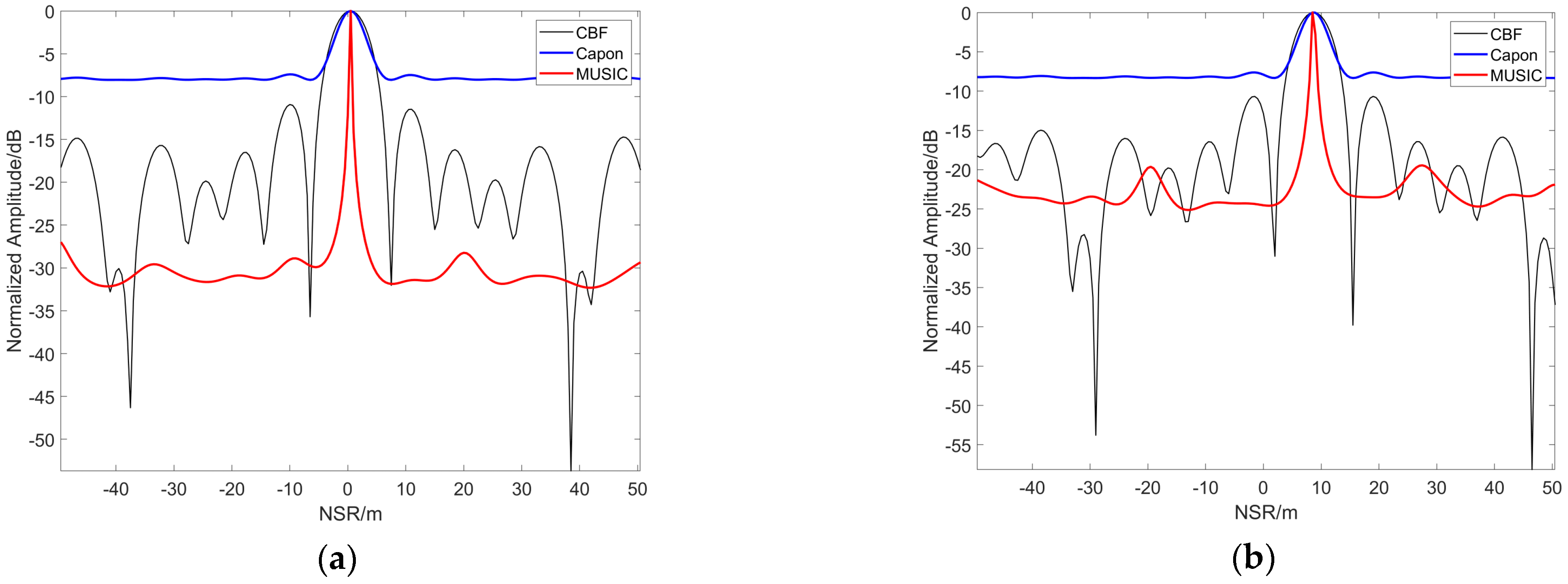
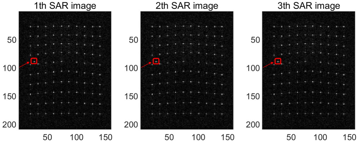
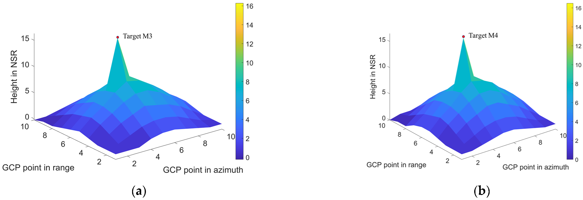
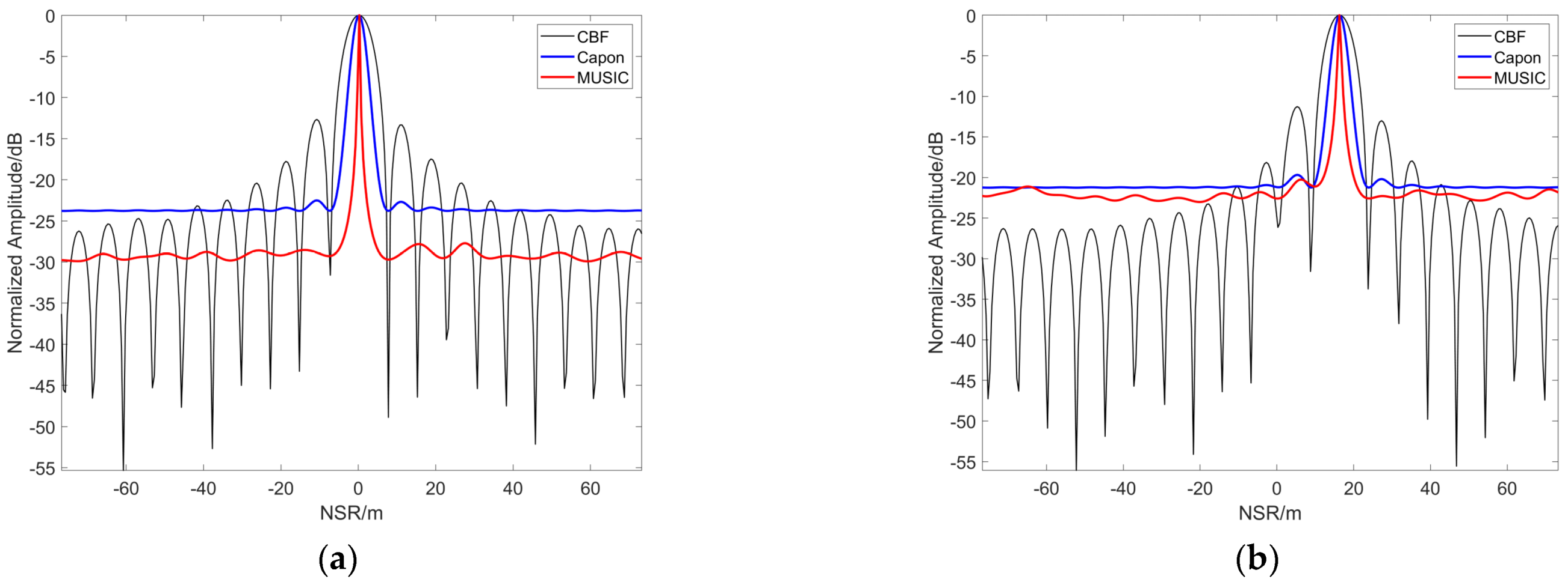
3.2.2. Static Target by Spectral Estimation
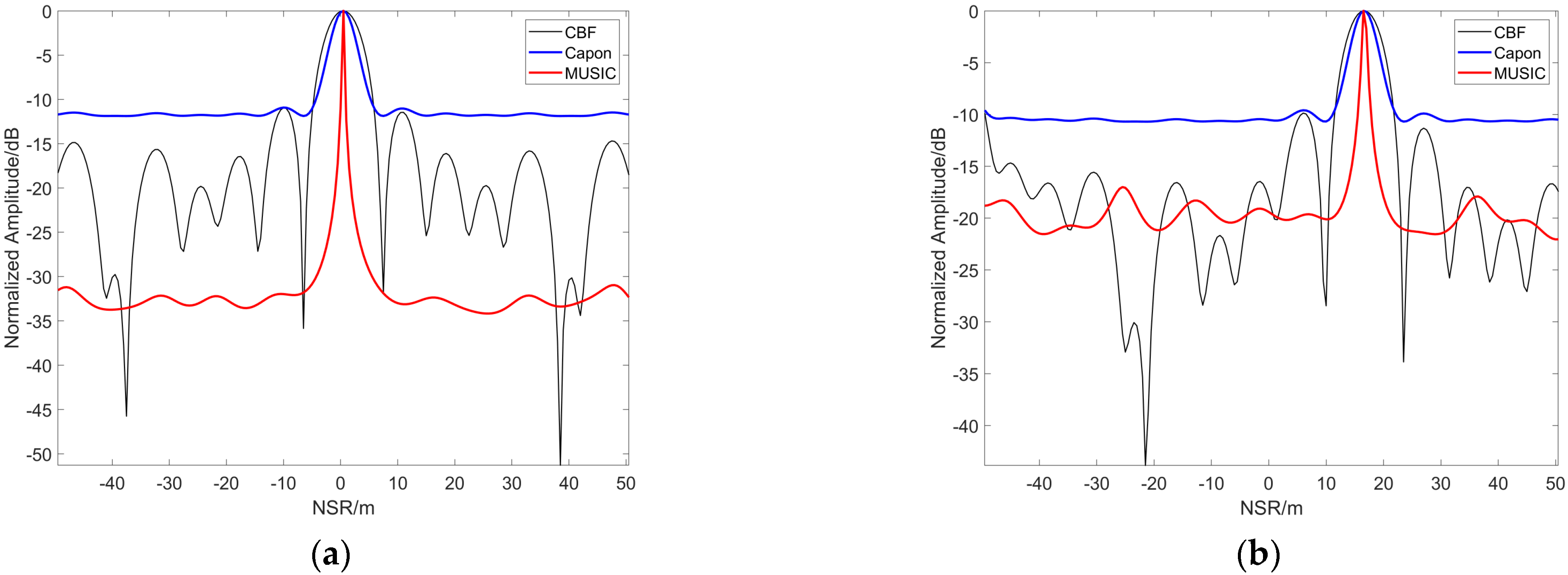
3.2.3. A Moving Target by Spectral Estimation
3.3. Simulation Evaluation
4. Discussion
5. Conclusions
Author Contributions
Funding
Data Availability Statement
Acknowledgments
Conflicts of Interest
Appendix A
Appendix B
References
- Pi, Y.M.; Yang, J.Y.; Fu, Y.S.; Yang, X.B. Synthetic Aperture Radar Imaging Principle; University of Electronic Science and Technology Press: Chengdu, China, 2007; pp. 50–60. [Google Scholar]
- Candes, E.J.; Tao, T. Near optimal signal recovery from random projections: Universal encoding strategies. IEEE Trans. Inf. Theory 2006, 52, 5406–5425. [Google Scholar] [CrossRef]
- Baumgartner, S.V.; Krieger, G. Multi-Channel SAR for Ground Moving Target Indication. In Academic Press Library in Signal Processing: Communications and Radar Signal Processing; Elsevier Science Publishers: Amsterdam, The Netherlands, 2014; pp. 911–986. [Google Scholar] [CrossRef]
- Zhang, S.X.; Gao, Y.X.; Xing, M.D.; Guo, R.; Chen, J.L.; Liu, Y.Y. Ground moving target indication for the geosynchronous-low Earth orbit bistatic multichannel SAR system. IEEE J. Sel. Top. Appl. Earth Observ. Remote Sens. 2021, 14, 5072–5090. [Google Scholar] [CrossRef]
- Wen, X.J.; Qiu, X.L. Research on turning motion targets and velocity estimation in high resolution spaceborne SAR. Sensors 2020, 20, 2201. [Google Scholar] [CrossRef] [PubMed]
- Zhang, Y.; Xiong, W.; Dong, X.; Hu, C. A novel azimuth spectrum reconstruction and imaging method for moving targets in geosynchronous spaceborne–airborne bistatic multichannel SAR. IEEE Trans. Geosci. Remote Sens. 2020, 58, 5976–5991. [Google Scholar] [CrossRef]
- Duan, K.Q.; Chen, H.; Xie, W.C.; Wang, Y.L. Deep learning for high-resolution estimation of clutter angle-Doppler spectrum in STAP. IET Radar Sonar Navig. 2022, 16, 193–207. [Google Scholar] [CrossRef]
- Zhan, M.Y.; Huang, P.H.; Liu, X.Z.; Chen, J.L.; Gao, Y.S.; Liu, Z.L. Performance analysis of space-borne early warning radar for AMTI. In Proceedings of the 2019 6th Asia-Pacific Conference on Synthetic Aperture Radar (APSAR), Xiamen, China, 26–29 November 2019; pp. 1–6. [Google Scholar] [CrossRef]
- Li, X.; Deng, B.; Qin, Y.L.; Wang, H.Q.; Li, Y.P. The influence of target micromotion on SAR and GMTI. IEEE Trans. Geosci. Remote Sens. 2011, 49, 2738–2751. [Google Scholar] [CrossRef]
- Zheng, L.F.; Zhang, S.S.; Zhang, X.Q. A novel strategy of 3D imaging on GEO SAR based on multi-baseline system. In Proceedings of the 2017 IEEE International Geoscience and Remote Sensing Symposium (IGARSS), Fort Worth, TX, USA, 23–28 July 2017; pp. 1724–1727. [Google Scholar] [CrossRef]
- Knaell, K.K.; Cardillo, G.P. Radar tomography for the generation of three-dimensional images. IEE Eng. Radar Sonar Navig. 1995, 142, 54–60. [Google Scholar] [CrossRef]
- Fabrizio, L. Differential tomography: A new framework for SAR interferometry. IEEE Trans. Geosci. Remote Sens. 2005, 43, 37–44. [Google Scholar] [CrossRef]
- Budillon, A.; Johnsy, A.C.; Schirinzi, G. Extension of a Fast GLRT Algorithm to 5D SAR Tomography of Urban Areas. Remote Sens. 2017, 9, 844. [Google Scholar] [CrossRef]
- Ferrara, M.; Jackson, J.; Stuff, M. Three-dimensional sparse-aperture moving-target imaging. In Proceedings of the Algorithms for Synthetic Aperture Radar Imagery XV, Orlando, FL, USA, 16–20 March 2008; pp. 49–59. [Google Scholar] [CrossRef]
- Sakamoto, T.; Matsuki, Y.; Sato, T. Method for the three-dimensional imaging of a moving target using an ultra-wideband radar with a small number of antennas. IEICE Trans. Commun. 2012, 95, 972–979. [Google Scholar] [CrossRef]
- Wang, P.F.; Liu, M.; Wang, S.W.; Li, Y.J.; Tang, K. 3D Velocity Estimation for Moving Targets via Geosynchronous Bistatic SAR. In Proceedings of the 2018 China International SAR Symposium (CISS), Shanghai, China, 10–12 October 2018; pp. 1–5. [Google Scholar] [CrossRef]
- Gui, S.L.; Li, J.; Zuo, F. Synthetic Aperture Radar Imaging Response of Three-dimensional Moving Target. In Proceedings of the 2019 6th Asia-Pacific Conference on Synthetic Aperture Radar (APSAR), Xiamen, China, 26–29 November 2019; pp. 1–4. [Google Scholar] [CrossRef]
- Lui, M.; Zhang, L.; Li, C.L. Nonuniform three-dimensional configuration distributed SAR signal reconstruction clutter suppression. Chin. J. Aeronaut. 2012, 25, 423–429. [Google Scholar] [CrossRef][Green Version]
- Yang, F.F. Spaceborne Radar GMTI System and Signal Processing Research. Ph.D. Thesis, National University of Defense Technology, Changsha, China, 2007. [Google Scholar]
- Zhou, L.; Yuan, J.Q.; Chen, A.L.; Hu, Z.M. Modeling and analysis of air target echo for space-based early warning radar. J. Air Force Early Warn. Acad. 2018, 32, 84–89. (In Chinese) [Google Scholar] [CrossRef]
- Fornaro, G.; Serafino, F.; Soldovieri, F. Three-dimensional focusing with multipass SAR data. IEEE Trans. Geosci. Remote Sens. 2003, 41, 507–517. [Google Scholar] [CrossRef]
- Sun, X.L. Research on SAR Tomography and Differential SAR Tomography Imaging Technology. Ph.D. Thesis, National University of Defense Technology, Changsha, China, 2012. [Google Scholar]
- Zhu, X.X.; Bamler, R. Very high resolution spaceborne SAR tomography in urban environment. IEEE Trans. Geosci. Remote Sens. 2010, 48, 4296–4308. [Google Scholar] [CrossRef]
- Lai, T. Study on HRWS Imaging Methods of Multi-channel Spaceborne SAR. Ph.D. Thesis, National University of Defense Technology, Changsha, China, 2010. [Google Scholar]
- Zhao, J.C.; Yu, A.X.; Zhang, Y.S.; Zhu, X.X.; Dong, Z. Spatial baseline optimization for spaceborne multistatic SAR tomography systems. Sensors 2019, 19, 2106. [Google Scholar] [CrossRef] [PubMed]
- Wei, L.H.; Feng, Q.Y.; Liu, S.J.; Bignami, C.; Tolomei, C.; Zhao, D. Minimum redundancy array—A baseline optimization strategy for urban SAR tomography. Remote Sens. 2020, 12, 3100. [Google Scholar] [CrossRef]
- Zhang, Y.S.; Liang, D.N.; Dong, Z. Analysis of time and frequency synchronization errors in spaceborne parasitic InSAR system. In Proceedings of the 2006 IEEE International Symposium on Geoscience and Remote Sensing, Denver, CO, USA, 31 July–4 August 2006; pp. 3047–3050. [Google Scholar] [CrossRef]
- Wang, Q.S.; Huang, H.H.; Yu, A.X.; Dong, Z. An efficient and adaptive approach for noise filtering of SAR interferometric phase images. IEEE Geosci. Remote Sens. Lett. 2011, 8, 1140–1144. [Google Scholar] [CrossRef]
- Wang, Q.S.; Huang, H.H.; Dong, Z.; Yu, A.X.; Liang, D.N. High-precision, fast DEM reconstruction method for spaceborne InSAR. Sci. China-Inf. Sci. 2011, 54, 2400–2410. [Google Scholar] [CrossRef][Green Version]
- Pan, J.; Wang, S.; Li, D.J.; Lu, X.C. High-resolution Wide-swath SAR moving target imaging technology based on distributed compressed sensing. J. Radars 2020, 9, 166–173. (In Chinese) [Google Scholar] [CrossRef]
- Ren, X.Z.; Qin, Y.; Tian, L.J. Three-dimensional imaging algorithm for tomography SAR based on multiple signal classification. In Proceedings of the 2014 IEEE International Conference on Signal Processing, Communications and Computing, Guilin, China, 5–8 August 2014; pp. 120–123. [Google Scholar] [CrossRef]
- Li, H.; Yin, J.; Jin, S.; Zhu, D.Y.; Hong, W.; Bi, H. Synthetic Aperture Radar Tomography in Urban Area Based on Compressive MUSIC. J. Phys. Conf. Ser. 2021, 2005, 012055. [Google Scholar] [CrossRef]
- Chen, Q.; Yu, A.X.; Sun, Z.Y.; Huang, H.H. A multi-mode space-borne SAR simulator based on SBRAS. In Proceedings of the 2012 IEEE International Geoscience and Remote Sensing Symposium, Munich, Germany, 22–27 July 2012; pp. 4567–4570. [Google Scholar] [CrossRef]
- Wang, M.; Liang, D.N.; Huang, H.H.; Dong, Z. SBRAS—An advanced simulator of spaceborne radar. In Proceedings of the 2007 IEEE International Geoscience and Remote Sensing Symposium, Barcelona, Spain, 23–27 July 2007; pp. 4942–4944. [Google Scholar] [CrossRef]


| a (km) | e | i (°) | Ω (°) | ω (°) | f (°) | |
|---|---|---|---|---|---|---|
| SC1 | 6893.38 | 0.00135 | 97.4478 | 295.305 | 66.7208 | 76.6798 |
| SC2 | 6893.38 | 0.00135 | 97.4481 | 295.305 | 67.0183 | 76.3823 |
| SC3 | 6893.38 | 0.00135 | 97.4484 | 295.306 | 67.3152 | 76.0854 |
| SC4 | 6893.38 | 0.00135 | 97.4487 | 295.306 | 67.6116 | 75.7890 |
| SC5 | 6893.38 | 0.00135 | 97.4490 | 295.307 | 67.9074 | 75.4932 |
| SC6 | 6893.38 | 0.00136 | 97.4493 | 295.307 | 68.2026 | 75.1980 |
| SC7 | 6893.38 | 0.00136 | 97.4496 | 295.308 | 68.4971 | 74.9035 |
| SC8 | 6893.38 | 0.00136 | 97.4499 | 295.308 | 68.7911 | 74.6096 |
| SC9 | 6893.38 | 0.00136 | 97.4502 | 295.308 | 69.0844 | 74.3163 |
| SC10 | 6893.38 | 0.00136 | 97.4505 | 295.309 | 69.3770 | 74.0237 |
| SC11 | 6893.38 | 0.00136 | 97.4508 | 295.309 | 69.6690 | 73.7317 |
| SC12 | 6893.38 | 0.00136 | 97.4511 | 295.310 | 69.9603 | 73.4405 |
| SC13 | 6893.38 | 0.00137 | 97.4514 | 295.310 | 70.2508 | 73.1499 |
| SC14 | 6893.38 | 0.00137 | 97.4517 | 295.311 | 70.5407 | 72.8600 |
| SC15 | 6893.38 | 0.00137 | 97.4520 | 295.311 | 70.8299 | 72.5709 |
| SC16 | 6893.38 | 0.00137 | 97.4523 | 295.312 | 71.1183 | 72.2824 |
| SC17 | 6893.38 | 0.00137 | 97.4526 | 295.312 | 71.4060 | 71.9948 |
| SC18 | 6893.38 | 0.00137 | 97.4529 | 295.313 | 71.6929 | 71.7078 |
| SC19 | 6893.38 | 0.00138 | 97.4532 | 295.313 | 71.9791 | 71.4217 |
| SC20 | 6893.38 | 0.00138 | 97.4535 | 295.314 | 72.2645 | 71.1363 |
| Parameter | Value |
|---|---|
| Baseline length | 1566 (m) |
| Band | X |
| Baseline number | 20 or 10 |
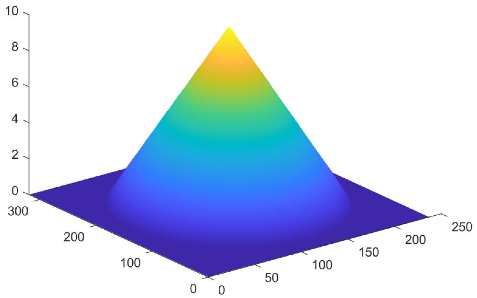
| Scene | Cone (radius 150 (m), height 10 (m)) |
| Initial target position | (0, , 8) (m) |
| Carry frequency | 9.6 (GHz) |
| Side-looking angle | 90° |
| Parameter | Value |
|---|---|
| PRF | 3785 (Hz) |
| Off-nadir angle | 36.52° |
| Receive signal sampling frequency | 160 (MHz) |
| Transmit signal bandwidth | 135 (MHz) |
| Peak power of the transmitted signal | 7680 (W) |
| Transmit signal pulse width | 4.7 × 10⁻⁵ (s) |
| Antenna azimuth size | 5.04 (m) |
| Antenna range dimension | 0.784 (m) |
| Observation Scene | Methods | Evaluation Performance | |||
|---|---|---|---|---|---|
| Time (s) (N = 20) | RMSE (N = 20) | Time (s) (N = 10) | RMSE (N = 10) | ||
| Static Cone | CBF | 0.8630 | 0.0182 | 0.8330 | 0.0227 |
| Moving Target (vx = 0.1 m/s) | 0.8282 | 0.0500 | 0.8209 | 0.0727 | |
| Moving Target (vx = 2.0 m/s) | 0.8200 | 0.8002 | 0.8164 | 0.8227 | |
| Static Cone | Capon | 0.8402 | 0.0182 | 0.8247 | 0.0227 |
| Moving Target (vx = 0.1 m/s) | 0.8078 | 0.0500 | 0.8047 | 0.0727 | |
| Moving Target (vx = 2.0 m/s) | 0.7870 | 0.8002 | 0.7855 | 0.8227 | |
| Static Cone | MUSIC | 0.8082 | 0.0182 | 0.7847 | 0.0227 |
| Moving Target (vx = 0.1 m/s) | 0.7824 | 0.0500 | 0.7744 | 0.0727 | |
| Moving Target (vx = 2.0 m/s) | 0.7783 | 0.8002 | 0.7706 | 0.8227 | |
Publisher’s Note: MDPI stays neutral with regard to jurisdictional claims in published maps and institutional affiliations. |
© 2022 by the authors. Licensee MDPI, Basel, Switzerland. This article is an open access article distributed under the terms and conditions of the Creative Commons Attribution (CC BY) license (https://creativecommons.org/licenses/by/4.0/).
Share and Cite
Han, Y.; Jiao, R.; Huang, H.; Wang, Q.; Lai, T. A Framework for Distributed LEO SAR Air Moving Target 3D Imaging via Spectral Estimation. Remote Sens. 2022, 14, 5956. https://doi.org/10.3390/rs14235956
Han Y, Jiao R, Huang H, Wang Q, Lai T. A Framework for Distributed LEO SAR Air Moving Target 3D Imaging via Spectral Estimation. Remote Sensing. 2022; 14(23):5956. https://doi.org/10.3390/rs14235956
Chicago/Turabian StyleHan, Yaquan, Runzhi Jiao, Haifeng Huang, Qingsong Wang, and Tao Lai. 2022. "A Framework for Distributed LEO SAR Air Moving Target 3D Imaging via Spectral Estimation" Remote Sensing 14, no. 23: 5956. https://doi.org/10.3390/rs14235956
APA StyleHan, Y., Jiao, R., Huang, H., Wang, Q., & Lai, T. (2022). A Framework for Distributed LEO SAR Air Moving Target 3D Imaging via Spectral Estimation. Remote Sensing, 14(23), 5956. https://doi.org/10.3390/rs14235956