Marine Extended Target Tracking for Scanning Radar Data Using Correlation Filter and Bayes Filter Jointly

Abstract

As the radar resolution improves, the extended structure of the targets in radar echoes can make a significant contribution to improving tracking performance, hence specific trackers need to be designed for these targets. However, traditional radar target tracking methods are mainly based on the accumulation of the target’s motion information, and the target’s appearance information is ignored. In this paper, a novel tracking algorithm that exploits both the appearance and motion information of a target is proposed to track a single extended target in maritime surveillance scenarios by incorporating the Bayesian motion state filter and the correlation appearance filter. The proposed algorithm consists of three modules. Firstly, a Bayesian module is utilized to accumulate the motion information of the target. Secondly, a correlation module is performed to capture the appearance features of the target. Finally, a fusion module is proposed to integrate the results of the former two modules according to the Maximum A Posteriori Criterion. In addition, a feedback structure is proposed to transfer the fusion results back to the former two modules to improve their stability. Besides, a scale adaptive strategy is presented to improve the tracker’s ability to cope with targets with varying shapes. In the end, the effectiveness of the proposed method is verified by measured radar data. The experimental results demonstrate that the proposed method achieves superior performance compared with other traditional algorithms, which simply focus on the target’s motion information. Moreover, this method is robust under complicated scenarios, such as clutter interference, target shape changing, and low signal-to-noise ratio (SNR).

1. Introduction

Radar extended target tracking technology is widely used in military and civilian fields, e.g., maritime target tracking. Traditional target tracking methods perform well based on the point target hypothesis, which is appropriate, as each target produces only one measurement per frame. Tracking filters are used to smooth the measured data during the scans, e.g., Kalman filter (KF) provides an optimal estimation for linear systems based on Gaussian and Markov assumptions [1]. Subsequently, for non-linear systems, several KF variants are proposed under the Gaussian assumption, including the Extended KF (EKF) [2] and the Unscented KF (UKF) [3]. Among them, the EKF ignores high order terms of the system’s state by linear approximation. The UKF reduces the estimation error by an unscented transform, which can effectively cope with highly non-linear environments. These methods use the accumulated detector data as input with the aim of iteratively calculating the posterior probability density function (PDF) of the target’s kinematic state. These techniques can be described within unified Bayes filter (BF) formalism [4]. However, traditional trackers are not suitable for an extended target, which may produce multiple measurements with noise, since the measurements of ship targets captured by the high-resolution radar working at scanning mode usually produce two-dimensional expansion in range and azimuth. The higher the radar’s range resolution, the more likely the extended target will generate measurements occupying multiple range resolution cells. In addition, if the radar working in scanning mode, the target may occupy multiple azimuth cells. Additionally, the resolution cell occupied by the target’s scattering point often changes due to the radar resolution, the reflection strength of the target or the change of the target’s attitude, which leads to the shape of some targets’ scattering point varying.

Recently, many methods are proposed for extended target tracking [5,6,7,8,9]. For example, Koch [5,6] utilized the random matrix model to describe the extension of the target appearance, and derived the analytical solutions under the Bayesian framework. Granstrom [8] proposed the extended target-Gaussian inverse Wishart-probability hypothesis density (ET-GIW-PHD) filter based on the RM (Random Matrices) model under the PHD framework. In addition, Granstrom [9] estimated the target’s motion state and shape by calculating the Gamma Gaussian inverse Wishart (GGIW) distribution of each target recursively. Marcus et al. [10,11] proposed Random Hypersurface Models to model extended targets. Random Hypersurface Models describe the target’s profile in terms of a parametric set of geometric shape functions, e.g., the Gaussian process model is one typical model [12]. Since each target generates multiple measurements, it is necessary to divide the measurements of the target. The algorithms mentioned above ensure reliability by traversing all divided measurements. However, the effect of measurement division is unsatisfactory when faced with the following challenging situations: overtaking, head-on meeting, and interruption clutter. Especially in maritime, strong sea clutter could interfere with the division of measurements. The clutter classified into the target cell always causes the association errors in the above methods, which results in severe degradation of the tracking performance. Although the extended target tracking methods mentioned above can estimate the shape of the target, the tracker only uses the motion information of the targets. In radar target tracking, the tracker usually only utilizes the position observation provided by the detector because the radar only captures one or more scatter points of the target. Intuitively, taking into account more available information would greatly improve the stability and accuracy of the tracker.

In addition to motion information, radar extended targets can also provide appearance information. Inspired by human visual instincts, some scholars introduce the amplitude information of the target into tracking methods which not only use the motion information but also take advantage of the appearance information of targets. Shui et al. [13] proposed a new approach to exploit three features of the received time series for detection of floating small targets in sea clutter. The difference in the statistical characteristics of amplitude between targets and clutters are used to improve the discrimination of them [14,15,16,17]. However, these feature-aided tracking methods need to extract features manually, and it is difficult to find a stable feature suitable for various complex maritime scenes.

The deep learning method, which has achieved remarkable results in computer vision, are also used to extract the features of radar targets by many scholars. Chen et al. [18] proposed to classify marine target and sea clutter by convolutional neural networks, which suggested that the above statistical learning methods are suitable for marine target detection and tracking, and the appearance of an extended target can provide useful features for detection. To achieve full utilization of the information contained in radar signals and improve the detection performance, Su et al. [19] utilized the graph convolutional network to detect marine radar targets. The above deep learning methods had achieved a very appealing performance on the real datasets. However, these methods require a large amount of data for offline training.

The kernel correlation filter (KCF) is an online learning method widely used in visual tracking [20], which can track the target in real time if given the training samples in the first frame. KCF [20] trains the filter based on the appearance information of the target in the current frame and the previous frame, and then performs correlation calculation with a new frame to track the appearance of the target. In order to handle the scale changing of the target, Danelljan et al. [21] proposed to learn discriminative correlation filters from a scale pyramid model, and Li et al. [22] gave a multiple scales searching strategy. Zhou et al. [23] introduced the correlation filtering method into radar target tracking for the first time, and proposed the Multiple Kernelized Correction Filter (MKCF) from the perspective of multi-kernel fusion, which performed satisfactorily in some challenging situations. It indicated that this correlation filter (CF) method is promising in radar target tracking [23]. Introducing the CF method into the traditional radar target tracking framework will help to improve the radar target tracking performance. However, most of these methods [23,24] treat the CF as a detector but not a tracker, which is not the best way to combine CF and the traditional radar target tracking framework.

To sum up, many existing methods for radar marine extended target tracking have been proven to be effective, but some of them suffer from poor robustness and incomplete use of observation information. Therefore, this paper attempts to make full use of the limited observation information of the radar targets adaptively. A new algorithm called JCBF is proposed to track a single maritime radar extended target utilizing both the motion and appearance information by jointing correlation filter and Bayes filter (JCBF). The proposed algorithm consists of three main parts: (1) Bayes filter (BF) is used to estimate the target’s motion state; (2) CF calculates the likelihood PDF of the target’s position using the real-time appearance features from the perspective of signal estimation; and (3) the final estimation of the target’s state is obtained by fusing the results of both filters from maximum a posteriori estimation criterion. In addition, a specific scaling pool for radar signals is also proposed to accommodate the extensions in distance and azimuth of targets. Finally, the experiments are performed on the scanning data collected by X-band marine radar to verify the proposed algorithm.

The main contributions of this paper are as follows. Firstly, a novel and specific tracker is designed for the radar target by jointing the BF and CF from an a posteriori probability perspective. Secondly, a strategy that can adapt to the target’s shape is employed to track the targets with varying shape. Finally, the experiments on real data sets demonstrate that the proposed method improves the stability of the tracker under low signal-to-clutter/noise ratio environments.

Table 1. Table of notations.

${\mathit{I}}_{\mathit{p}}$	Identity matrix of order p
${\mathit{O}}_p$	p × p matrix with zero entries
${\left(·\right)}^T$	Transpose
${\left(·\right)}^H$	Conjugate transpose
${\left(·\right)}^{\ast }$	Conjugate
$\left|·\right|$	Module of a vector
$∥·∥$	Frobenius norm of a matrix
$det\left(·\right)$	Determinant of a matrix
$\mathcal{F}\left(·\right)$	Fourier transform
${\mathcal{F}}^{-1}\left(·\right)$	Inverse Fourier transform
$mean\left(·\right)$	Mean
⊙	Hadamard product
$〈·,·〉$	Inner product
$\mathcal{N}\left(\mathit{x};\mathit{m},\sum \right)$	$\frac{1}{\sqrt{2\pi det\left(\sum \right)}}exp\left\{-\frac{1}{2}{\left(\mathit{x}-\mathit{m}\right)}^T{\sum }^{-1}\left(\mathit{x}-\mathit{m}\right)\right\}$

gives a list of notations used throughout the paper.

2. Proposed JCBF

This section begins with a brief introduction to the basic principles of BF [4] and KCF [20]. Next, the theoretical derivation and a specific implementation of the integrated BF and CF approach are given in Section 2.3 and Section 2.4, respectively, where the viewpoint in [23] that analyzing the KCF in the perspective of probability is highlighted. Following that, two strategies for improving the robustness of the tracker are given in Section 2.5 where a feedback structure is suggested to pass the fusion outcomes back to the former BF and KCF to improve their stability, and a scale adaptive strategy is presented to ameliorate the robustness of the tracker against shape-changing targets. Finally, the proposed method is summarized in Section 2.6.

2.1. Bayesian Framework

Assuming that the state equation and the observation equation of the system (linear or nonlinear system) are as follows:

$${\mathit{x}}_{k+1}={\mathit{f}}_k\left({\mathit{x}}_k\right)+{\mathit{u}}_k,$$

(1)

$${\mathit{z}}_k={\mathit{h}}_k\left({\mathit{x}}_k\right)+{\mathit{n}}_k,$$

(2)

where $k\in \mathbb{N}$ denotes the time step, ${\mathit{x}}_k\in {\mathbb{R}}^n$ is the system state vector at time k, ${\mathit{f}}_k:{\mathbb{R}}^n\to {\mathbb{R}}^n$ denotes the state transition map, ${\mathit{u}}_k$ is the process noise, ${\mathit{z}}_k\in {\mathbb{R}}^m$ is the measurement vector at time k, ${\mathit{h}}_k:{\mathbb{R}}^n\to {\mathbb{R}}^m$ denotes the measurement map ($n>m$), and ${\mathit{n}}_k$ is the measurement noise. Note that ${\mathit{f}}_k$ and ${\mathit{h}}_k$ can denote both linear and nonlinear maps.

The Bayes filter uses the measurements set ${\mathit{Z}}^k$ ($\left[{\mathit{z}}_1,{\mathit{z}}_2,\dots ,{\mathit{z}}_k\right]$) to calculate the PDF of the state ${\mathit{x}}_k$ at time k, i.e., $p\left({\mathit{x}}_k|{\mathit{Z}}^k\right),k\in \mathbb{N}$. The steps of the Bayes filter are divided into prediction and update, as follows:

• Assuming that $p\left({\mathit{x}}_{k-1}|{\mathit{Z}}^{k-1}\right)$ has been obtained at time k − 1, then the PDF of the one-step predictions of the state and measurement are (3) and (4), respectively:

  $$p\left({\mathit{x}}_k|{\mathit{Z}}^{k-1}\right)={\int }_{{\mathbb{R}}^n}p\left({\mathit{x}}_k|{\mathit{x}}_{k-1}\right)p\left({\mathit{x}}_{k-1}|{\mathit{Z}}^{k-1}\right)d{\mathit{x}}_{k-1},$$

  (3)

  $$p\left({\mathit{z}}_k|{\mathit{Z}}^{k-1}\right)={\int }_{{\mathbb{R}}^n}p\left({\mathit{z}}_k|{\mathit{x}}_k\right)p\left({\mathit{x}}_k|{\mathit{Z}}^{k-1}\right)d{\mathit{x}}_k,$$

  (4)

  where $p\left({\mathit{x}}_k|{\mathit{x}}_{k-1}\right)$ and $p\left({\mathit{z}}_k\right|{\mathit{x}}_k)$ are given by (1) and (2), respectively.
• The posterior PDF is calculated using the new measurement ${\mathit{z}}_k$ obtained at time k [4]:

  $$p\left({\mathit{x}}_k|{\mathit{Z}}^k\right)=\frac{p\left({\mathit{z}}_k|{\mathit{x}}_k\right)p\left({\mathit{x}}_k|{\mathit{Z}}^{k-1}\right)}{p\left({\mathit{z}}_k|{\mathit{Z}}^{k-1}\right)}.$$

  (5)

2.2. Kernal Correlation Filter

KCF [20] solves the classifier by means of ridge regression. In the initial linear regression model, the optimization objective function is (6). Given the training feature-label pairs $\{{\mathit{g}}_i,y_i\}$, the loss function is as in (7):

$$f\left({\mathit{g}}_i\right)={\mathit{w}}^T{\mathit{g}}_i,$$

(6)

$$\underset{\mathit{w}}{min}\sum _i{(f\left({\mathit{g}}_i\right)-{\mathit{y}}_i)}^2+\lambda {∥\mathit{w}∥}^2.$$

(7)

Assuming that $\mathit{G}={[{\mathit{g}}_1,{\mathit{g}}_2,\dots ,{\mathit{g}}_n]}^T$ denotes n training samples and $\mathit{y}={[{\mathit{y}}_1,\dots ,{\mathit{y}}_n]}^T$ denotes their labels, it can be derived that w has a closed-form solution $\mathit{w}={({\mathit{G}}^H\mathit{G}+\lambda \mathit{I})}^{-1}{\mathit{G}}^H\mathit{y}$.

To improve the classifier’s performance, the data in original space are mapped to a high-dimensional space with weights w as linear combinations of the input samples:

$$\mathit{w}=\sum _i{\alpha }_i\phi \left({\mathit{g}}_i\right).$$

(8)

When putting the w in the optimization process, the detailed form of function $\phi (·)$ is not necessary, only the inner product of $\phi (·)$ is needed, i.e., $k\left({\mathit{g}}_i,{\mathit{g}}_j\right)=〈\phi \left({\mathit{g}}_i\right),\phi \left({\mathit{g}}_j\right)〉$.

By introducing the kernel function $k({\mathit{g}}_i,{\mathit{g}}_j)=exp\left(-\frac{1}{{\sigma }_k^2}\left({∥{\mathit{g}}_i∥}^2+{∥{\mathit{g}}_j∥}^2-2{\mathit{g}}_i^T{\mathit{g}}_j\right)\right)$, and putting it and weights (8) into (7), the optimal solution can be converted to (9):

$$\mathit{\alpha }={(\mathit{K}+\lambda \mathit{I})}^{-1}\mathit{y},$$

(9)

where $\mathit{\alpha }={[{\alpha }_1,\dots ,{\alpha }_n]}^T$, K is a circular matrix with $n\times n$ dimensions, and ${\mathit{K}}_{ij}=k({\mathit{g}}_i,{\mathit{g}}_j)$.

Since K is a circular matrix, (9) can be converted into $\mathit{\alpha }={\mathcal{F}}^{-1}\left(\frac{\mathcal{F}\left(\mathit{y}\right)}{{\mathcal{F}}^{\ast }\left({\mathit{k}}_{gg}\right)+\lambda }\right)$, where ${\mathit{k}}_{gg}$ denotes the first row of the circular matrix K [20].

After training the model using sample g in the last frame, the response of the new input sample g′ in the new frame is computed by:

$$\mathit{Y}={\mathcal{F}}^{-1}\left(\mathcal{F}\left({\mathit{k}}_{g{g}^{\prime }}\right)\odot \mathcal{F}\left(\mathit{\alpha }\right)\right).$$

(10)

Let v be the position variable of the target at a certain time step, the position v of the target is the position of the maximum value in the response $\mathit{Y}\left(\mathit{v}\right)$, which can be given by:

$$\widehat{\mathit{v}}=arg\underset{\mathit{v}}{max}\mathit{Y}\left(\mathit{v}\right)$$

(11)

The model is updated by (12), where ${\mathit{g}}_t$ and ${\mathit{\alpha }}_t$ denote the training sample and the weights at time t, ${\mathit{g}}_t^{\prime }$ and ${\mathit{\alpha }}_{{\mathit{g}}_t^{\prime }}$ denote the new sample and the new weights, and $\eta \in (0,1)$ denotes forgetting rate [23].

$$\left\{\begin{array}{c}{\mathit{g}}_t={\mathit{g}}_t^{\prime }\times \eta +{\mathit{g}}_{t-1}\times (1-\eta )\hfill \\ {\mathit{\alpha }}_t={\mathit{\alpha }}_{{\mathit{g}}_t^{\prime }}\times \eta +{\mathit{\alpha }}_{t-1}\times (1-\eta )\hfill \end{array}\right.$$

(12)

2.3. Joint Correlation and Bayes Filtering

In order to make full use of the target’s appearance and motion information to estimate the target’s position ${\mathit{v}}_k\in {\mathbb{R}}^m$, the posterior PDF $p\left({\mathit{v}}_k|{\mathit{Z}}^k,{\mathit{A}}^k\right)$ of ${\mathit{v}}_k$ at time k is calculated utilizing both the obtained position measurement ${\mathit{z}}_k$ and the appearance measurement ${\mathit{a}}_k$, where ${\mathit{A}}_k$ ($\left[{\mathit{a}}_1,{\mathit{a}}_2,\dots ,{\mathit{a}}_k\right]$) denotes the appearance measurements set.

Further discussion will be much simplified if additionally assuming that the position of the target and the appearance feature of the target are independent of each other. Such an assumption seems to be justified in many practical cases, as follows:

$$p\left({\mathit{Z}}^k,{\mathit{A}}^k|{\mathit{v}}_k\right)=p\left({\mathit{Z}}^k|{\mathit{v}}_k\right)p\left({\mathit{A}}^k|{\mathit{v}}_k\right),$$

(13)

$$p\left({\mathit{Z}}^k,{\mathit{A}}^k\right)=p\left({\mathit{Z}}^k\right)p\left({\mathit{A}}^k\right).$$

(14)

Therefore, the posterior PDF of the state ${\mathit{v}}_k$ is given by:

$$\begin{array}{cc}p\left({\mathit{v}}_k|{\mathit{Z}}^k,{\mathit{A}}^k\right)& =\frac{p\left({\mathit{Z}}^k,{\mathit{A}}^k|{\mathit{v}}_k\right)p\left({\mathit{v}}_k\right)}{p\left({\mathit{Z}}^k,{\mathit{A}}^k\right)}\\ & =\frac{p\left({\mathit{Z}}^k|{\mathit{v}}_k\right)p\left({\mathit{A}}^k|{\mathit{v}}_k\right)p\left({\mathit{v}}_k\right)}{p\left({\mathit{Z}}^k\right)p\left({\mathit{A}}^k\right)}\\ & =\frac{p\left({\mathit{v}}_k|{\mathit{Z}}^k\right)p\left({\mathit{A}}_k|{\mathit{v}}^k\right)}{p\left({\mathit{A}}_k\right)}\\ & \propto p\left({\mathit{v}}_k|{\mathit{Z}}^k\right)p\left({\mathit{A}}_k|{\mathit{v}}^k\right).\end{array}$$

(15)

Zhou et al. [23] firstly analyze the KCF in the perspective of maximum likelihood. They propose that the response (10) can be viewed as the more advanced likelihood function whose strength shows the probability of the target at each position $\mathit{v}$. Hence, given a position ${\mathit{v}}_k\in {\mathbb{R}}^m$, the probability of ${\mathit{v}}_k$ being the center of the target measured by KCF is the individual likelihood $p\left({\mathit{A}}_k|v^k\right)$, where the ${\mathit{A}}_k$ denotes the appearance measurements obtained by KCF. Treating the response of KCF as an appearance measurement captured by one sensor, KCF can be considered as a filter that utilizes the target’s real-time appearance measurements ${\mathit{A}}_k$ to calculate the likelihood PDF of the target’s position ${\mathit{v}}_k$.

In KCF, the response matrix is equal to the individual likelihood distribution of ${\mathit{v}}_k$ [23], thus $p\left(A_k|v^k\right)$ in (15) can be calculated by KCF:

$$p\left({\mathit{A}}_k|v^k\right)=\mathit{Y}\left(\mathit{v}\right)$$

(16)

As discussed in Section 2.1, BF calculates the posterior PDF $p\left({\mathit{x}}_k|Z^k\right)$ of ${\mathit{x}}_k\in {\mathbb{R}}^n$ using the obtained measurement ${\mathit{z}}_k\in {\mathbb{R}}^m$ and $p\left({\mathit{x}}_{k-1}|Z^{k-1}\right)$.

The state estimation ${\mathit{v}}_k\in {\mathbb{R}}^m$ of the target’s position is a fraction of ${\mathit{x}}_k$, thus ${\mathit{x}}_k$ can be decomposed into two components as ${\mathit{x}}_k={\left[{\mathit{v}}_k,{\mathit{e}}_k\right]}^T$, where ${\mathit{e}}_k\in {\mathbb{R}}^{n-m}$. As a result, $p\left({\mathit{v}}_k|Z^k\right)$ is given by (17):

$$\begin{array}{cc}p\left({\mathit{v}}_k|Z^k\right)& =\int p\left({\mathit{v}}_k,{\mathit{e}}_k|Z^k\right)d{\mathit{e}}_k\\ & =\int p\left({\mathit{x}}_k|Z^k\right)d{\mathit{e}}_k.\end{array}$$

(17)

Finally, $p\left({\mathit{v}}_k|Z^k,A^k\right)$ can be calculated by (15)–(17). As a result, the maximum a posteriori estimation (MAP) of ${\mathit{v}}_k$ is given by (18):

$$\begin{array}{cc}\hfill {\widehat{\mathit{v}}}_k& =arg\underset{{\mathit{v}}_k}{max}p\left({\mathit{v}}_k\right|{\mathit{Z}}^k,{\mathit{A}}^k)\hfill \\ & =arg\underset{{\mathit{v}}_k}{max}p\left({\mathit{v}}_k\right|{\mathit{Z}}^k)p\left({\mathit{A}}_k\right|{\mathit{v}}^k).\hfill \end{array}$$

(18)

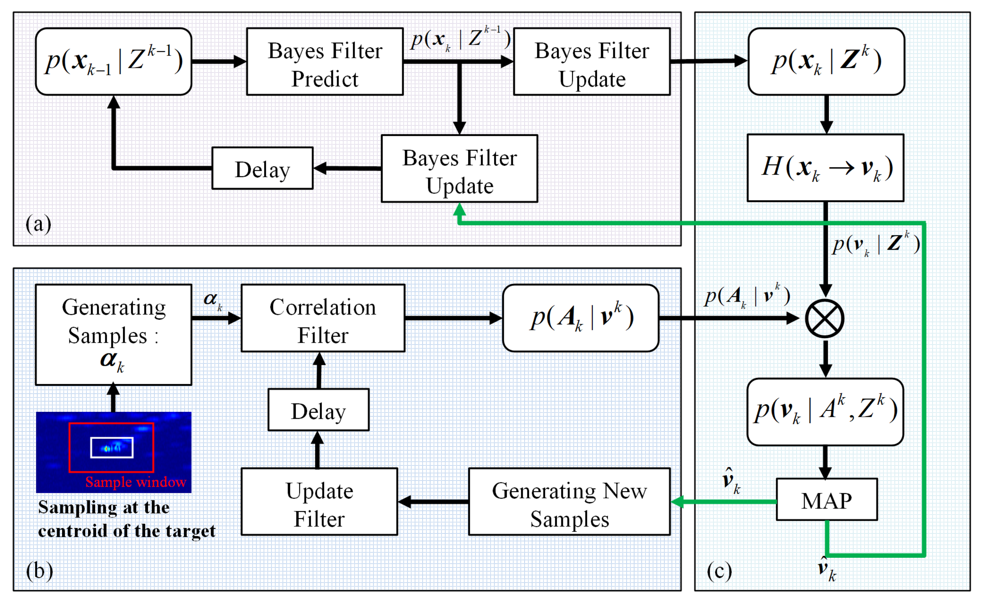
Not only the appearance information but also the motion information is successfully utilized in (18) to estimate the target’s position ${\mathit{v}}_k$ by jointing the Bayes filter and the Correlation filter. The overall flow of JCBF is shown in Figure 1, among which a fusion module (Figure 1c) is used to combine the BF module (Figure 1a) and the CF module Figure 1b.

2.4. Specific Implementation of JCBF

This section gives a specific implementation of JCBF. Since radar measurements are generally obtained from the distance and bearing of the target in the polar coordinate system, this paper constructs the equations of state and observation in the polar coordinate system and implements the proposed tracking algorithm.

2.4.1. Bayes Filter Module

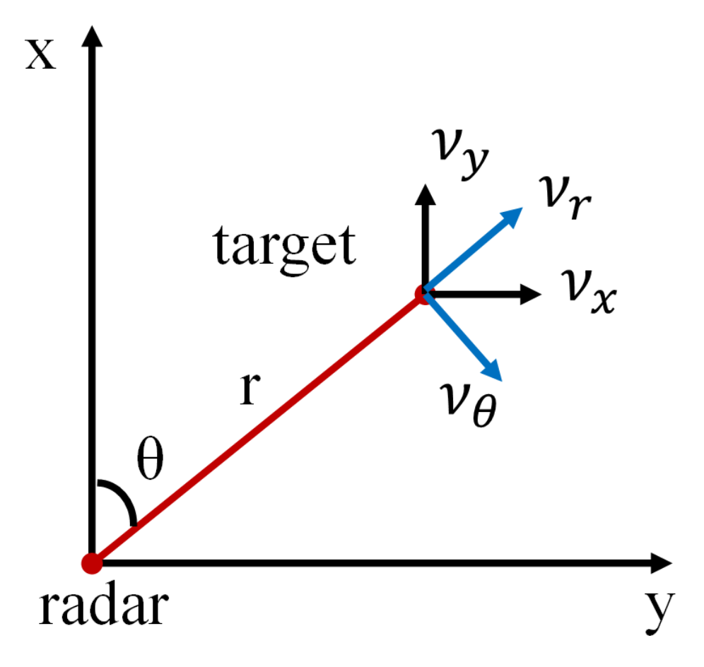
In the polar coordinate, the motion state of the target can be represented by ${\mathit{x}}_k={\left[r,\theta ,{\nu }_r,{\nu }_{\theta }\right]}^T$, where r denotes the radial range between the target and the radar, θ denotes the azimuth, ${\nu }_r$ denotes the radial velocity and ${\nu }_{\theta }$ denotes the tangential velocity. The measurement can be represented by ${\mathit{z}}_k={\left[r,\theta \right]}^T$.

Due to the weak manoeuvrability of most maritime targets, for the sake of simplicity, this paper assumes that the target’s motion model conforms to a Nearly Constant Velocity (NCV) motion model in the Cartesian coordinate. Assuming that the radar’s scanning period is T, the above motion model and the observation equation in the polar coordinate system can be represented as follows [25]:

$${\mathit{x}}_{k+1}={\mathit{f}}_k\left({\mathit{x}}_k\right)+{\mathit{u}}_k,$$

(19)

$${\mathit{z}}_k={\mathit{H}}_k{\mathit{x}}_k+{\mathit{n}}_k,$$

(20)

where

$${\mathit{f}}_k\left(·\right)=\left[\begin{array}{c}\sqrt{{\left(rcos\theta +({\nu }_{r}cos\theta -{\nu }_{\theta }sin\theta )T\right)}^2+{\left(rsin\theta +({\nu }_{r}sin\theta +{\nu }_{\theta }cos\theta )T\right)}^2}\\ arctan\left(\frac{rsin\theta +({\nu }_{r}sin\theta +{\nu }_{\theta }cos\theta )T}{rcos\theta +({\nu }_{r}cos\theta -{\nu }_{\theta }sin\theta )T}\right)\\ ({\nu }_{r}sin\theta +{\nu }_{\theta }cos\theta )sin\theta +({\nu }_{r}cos\theta -{\nu }_{\theta }sin\theta )cos\theta \\ ({\nu }_{r}sin\theta +{\nu }_{\theta }cos\theta )cos\theta -({\nu }_{r}cos\theta -{\nu }_{\theta }sin\theta )sin\theta \end{array}\right],$$

(21)

$${\mathit{H}}_k=\left[\begin{array}{cccc}1& 0& 0& 0\\ 0& 1& 0& 0\end{array}\right].$$

(22)

Since the motion Equation (19) is a nonlinear model, this paper utilizes EKF [2] to estimate the state ${\mathit{x}}_k$. The detailed calculation process of EKF and the derivation of (21) are displayed in Appendix A and Appendix B, respectively.

Given the measurements ${\mathit{Z}}^k$, EKF iteratively calculates the first moment and second moment of ${\mathit{x}}_k\in {\mathbb{R}}^n$, and approximates the posterior PDF of ${\mathit{x}}_k$ to a Gaussian distribution:

$$p\left({\mathit{x}}_k|{\mathit{Z}}^k\right)=\mathbb{R}\left({\mathit{x}}_k;{\mathit{m}}_{\mathit{x}},{\sum }_{\mathit{x}}\right).$$

(23)

where ${\mathit{m}}_{\mathit{x}}$ denotes the mean of ${\mathit{x}}_k$ and ${\sum }_{\mathit{x}}$ denotes the covariance matrix. The expressions for ${\mathit{x}}_k$ and ${\sum }_{\mathit{x}}$ are displayed in Appendix A.

As discussed in Section 2.3, the key is to solve for the posterior PDF of ${\mathit{v}}_k$ as (15). In the motion model (19), ${\mathit{v}}_k$ denotes the range and azimuth where the target is located, i.e., ${\mathit{v}}_k={\left[r,\theta \right]}^T$. Consequently, ${\mathit{x}}_k={\left[r,\theta ,{\nu }_r,{\nu }_{\theta }\right]}^T$ can be decomposed into two components as ${\mathit{x}}_k={\left[{\mathit{v}}_k,{\mathit{e}}_k\right]}^T$, where ${\mathit{e}}_k={\left[{\nu }_r,{\nu }_{\theta }\right]}^T$. Plugging (23) into (17), the posterior PDF of the target’s position ${\mathit{v}}_k$ can be derived as:

$$\begin{array}{cc}p\left({\mathit{v}}_k|Z^k\right)\hfill & =\int \mathcal{N}\left({\mathit{x}}_k;{\mathit{m}}_{\mathit{x}},{\sum }_{\mathit{x}}\right)d{\mathit{e}}_k\hfill \\ & =\int \frac{1}{\sqrt{2\pi det\left({\sum }_x\right)}}exp\left\{-\frac{1}{2}{\left({\left[{\mathit{v}}_k,{\mathit{e}}_k\right]}^T-{\mathit{m}}_x\right)}^T{{\sum }_x}^{-1}\left({\left[{\mathit{v}}_k,{\mathit{e}}_k\right]}^T-{\mathit{m}}_x\right)\right\}d{\mathit{e}}_k\hfill \\ & =\frac{1}{\sqrt{2\pi det\left({\sum }_1\right)}}exp\left\{-\frac{1}{2}{\left({\mathit{v}}_k-{\mathit{m}}_1\right)}^T{\sum }_1^{-1}\left({\mathit{v}}_k-{\mathit{m}}_1\right)\right\}\hfill \\ & =\mathcal{N}\left({\mathit{v}}_k;{\mathit{m}}_1,{\sum }_1\right),\hfill \end{array}$$

(24)

where ${\mathit{m}}_1=\mathit{H}{\mathit{m}}_{\mathit{x}}$, ${\sum }_1=\mathit{H}{\sum }_{\mathit{x}}{\mathit{H}}^T$ and $\mathit{H}=\left[{\mathit{I}}_2,{\mathit{O}}_2\right]$.

2.4.2. Correlation Filter Module

The training labels of KCF are two-dimensional (2D) needle-shaped Gaussian [20,23], if the test sample is similar with the train samples, the response $f\left({\mathit{a}}_k\right)$ of KCF given by () is a similar needle-shaped Gaussian to the training labels. Thus, the position ${\mathit{v}}_k$ can be assumed to obey 2d Gaussian distribution, and such an assumption simplifies the further discussion and is reasonable in most cases. As discussed in Section 2.3, given the ${\mathit{A}}_k$, the likelihood PDF of position variable ${\mathit{v}}_k$ is computed by:

$$p\left({\mathit{A}}_k|{\mathit{v}}^k\right)=\mathcal{N}\left({\mathit{v}}_k;{\mathit{m}}_2,{\sum }_2\right),$$

(25)

where ${\mathit{m}}_2=\mathit{\mu }$ and ${\sum }_2={\sigma }^2{\mathit{I}}_m$. For KCF, $\mathit{\mu }$ denotes the location of the maximum value $y_p$ in the response map, and ${\sigma }^2$ is inversely proportional to the $y_p$, i.e., ${\sigma }^2=\frac{1}{2\pi y_p}$.

2.4.3. Fusion Module

This module calculates the maximum posterior estimate of the target location by fusing the results of the above two modules.

$p\left({\mathit{v}}_k|{\mathit{Z}}^k\right)p\left({\mathit{A}}_k|{\mathit{v}}^k\right)$ is given by:

$$\begin{array}{cc}p\left({\mathit{v}}_k|{\mathit{Z}}^k\right)p\left({\mathit{A}}_k|{\mathit{v}}^k\right)& =\mathcal{N}\left({\mathit{v}}_k;{\mathit{m}}_1,{\sum }_1\right)\mathcal{N}\left({\mathit{v}}_k;{\mathit{m}}_2,{\sum }_2\right)\hfill \\ & ={\mathit{C}}_c\mathcal{N}\left({\mathit{v}}_k;{\mathit{m}}_c,{\sum }_c\right),\hfill \end{array}$$

(26)

where

$${\sum }_c={\left({\sum }_1^{-1}+{\sum }_2^{-1}\right)}^{-1},$$

(27)

$${\mathit{m}}_c={\sum }_c\left({\sum }_1^{-1}{\mathit{m}}_1+{\sum }_2^{-1}{\mathit{m}}_2\right),$$

(28)

$${\mathit{C}}_c=\frac{1}{\sqrt{2\pi det\left({\sum }_1+{\sum }_2\right)}}exp\left\{-\frac{1}{2}{\left({\mathit{m}}_1-{\mathit{m}}_2\right)}^T{\left({\sum }_1+{\sum }_2\right)}^{-1}\left({\mathit{m}}_1-{\mathit{m}}_2\right)\right\}.$$

(29)

According to (18), the maximum a posterior estimation of ${\mathit{v}}_k$ can be derived as (30) and the covariance matrix of estimation errors is ${\sum }_c$.

$$\begin{array}{cc}{\widehat{\mathit{v}}}_k& =arg\underset{{\mathit{v}}_k}{max}p\left({\mathit{v}}_k\right|{\mathit{Z}}^k)p\left({\mathit{A}}_k\right|{\mathit{v}}^k)\hfill \\ & =arg\underset{{\mathit{v}}_k}{max}{\mathit{C}}_c\mathcal{N}\left({\mathit{v}}_k;{\mathit{m}}_c,{\sum }_c\right)\hfill \\ & ={\mathit{m}}_c\hfill \end{array}.$$

(30)

2.5. Strategies to Improve the Stability of Tracker

2.5.1. A Feedback Structure in the JCBF

A feedback module is introduced into the proposed method to improve the stability. The fused results given by JCBF are treated as corrected measurements to re-update BF and CF. The green lines in Figure 1 illustrate this process.

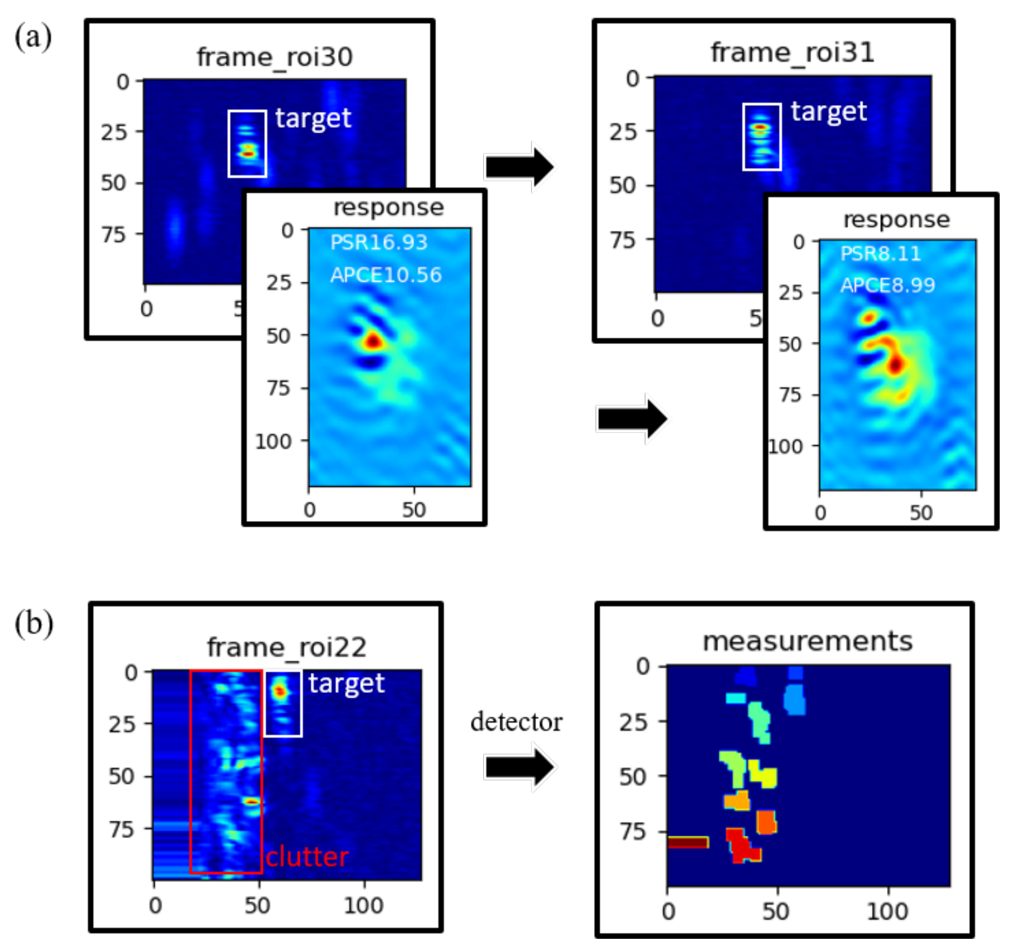
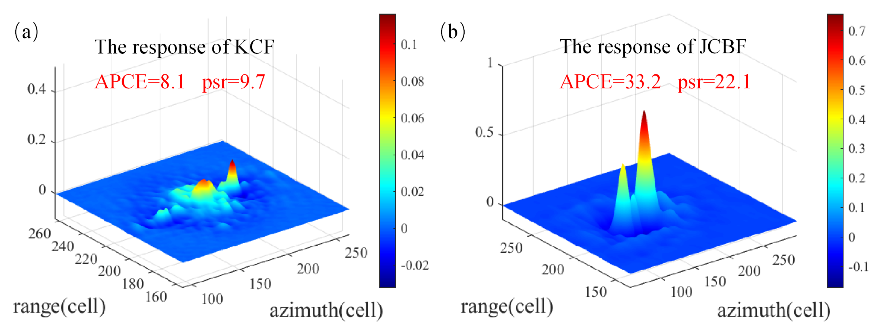
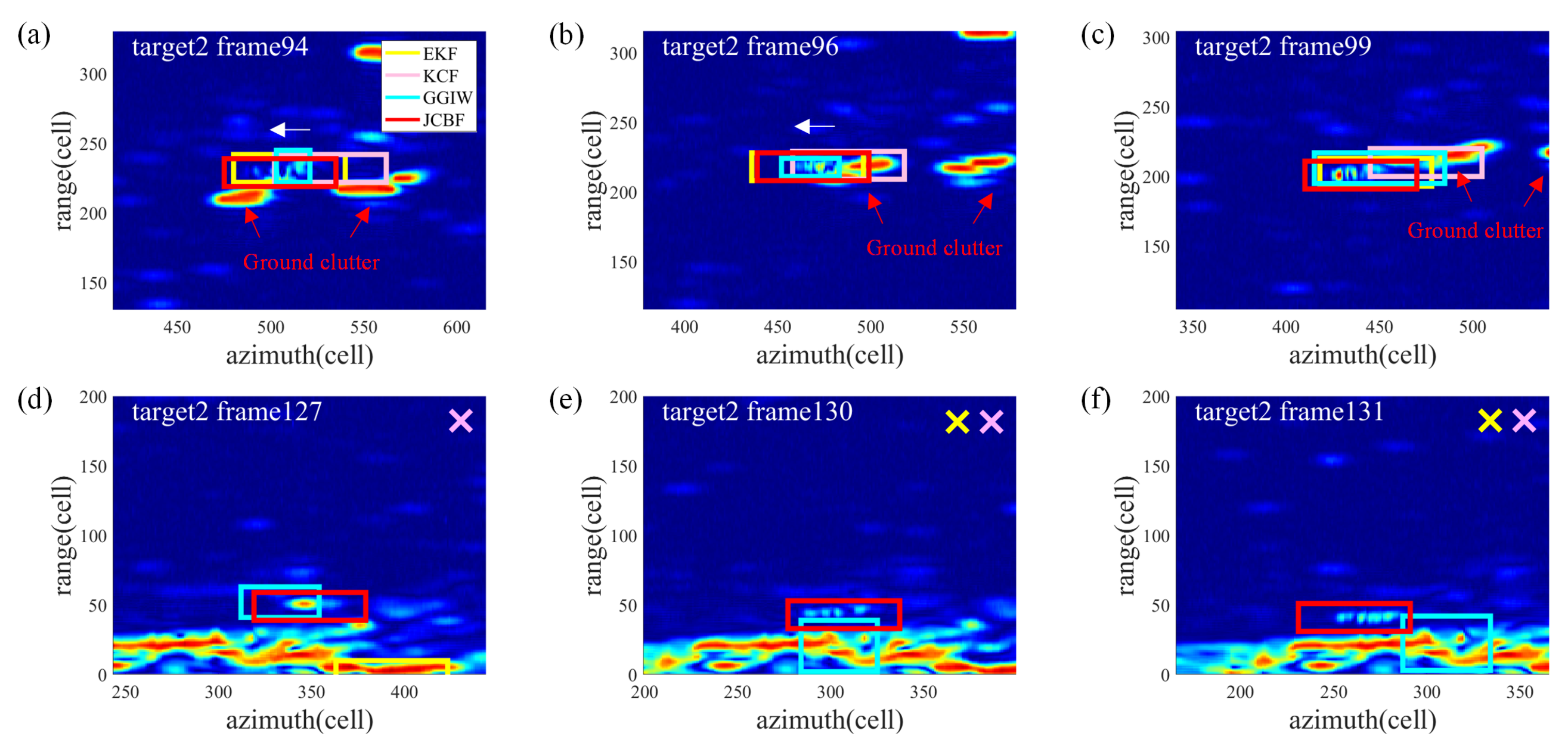
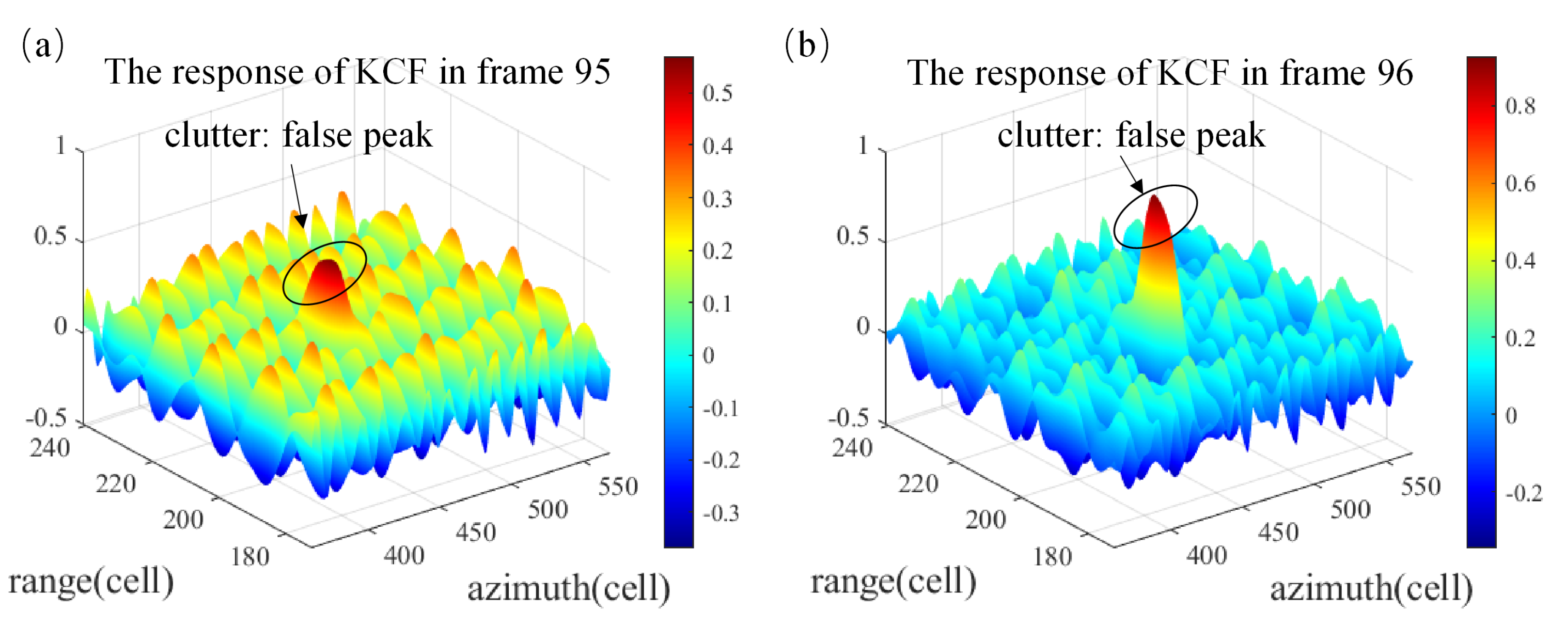
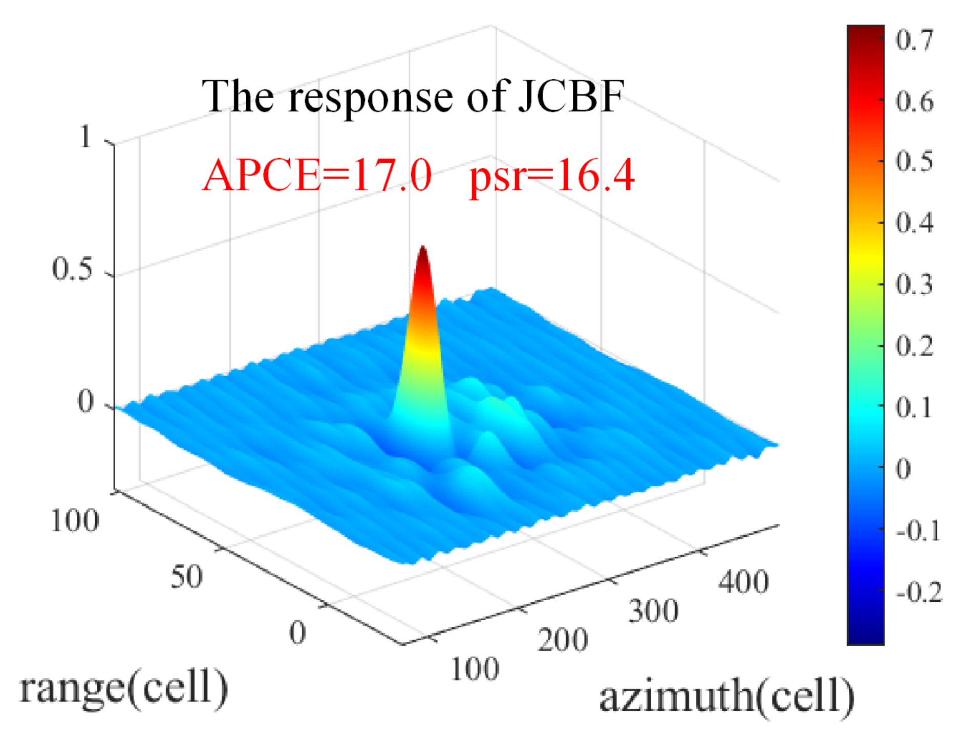
After capturing the target at time k, the correlation filter usually updates the model with new sample, as shown in (12). However, when the target is obscured by clutter or changes significantly in appearance, as shown in Figure 2a, the response of the filter deteriorates significantly, which leads to inaccurate estimation of the target state. The peak to side-lobe ratio (PSR) [26] and average peak-to-correlation energy (APCE) [27] are utilized to evaluate the fluctuated degree of response y and the confidence level of the detected targets, which are given by (31) and (32), respectively,

$$PSR=\frac{{\mathit{y}}_{max}-{\mu }_s}{{\sigma }_s},$$

(31)

$$APCE=\frac{{\left|{\mathit{y}}_{max}-{\mathit{y}}_{min}\right|}^2}{mean\left(\sum _{w,h}{\left({\mathit{y}}_{w,h}-{\mathit{y}}_{min}\right)}^2\right)},$$

(32)

where ${\mu }_s$ and ${\sigma }_s$ are the mean and standard deviation of the side-lobe, respectively, and ∑ denotes summation.

In this strategy, the reselected sample extracted from the estimated position given by the JCBF is utilized to update the CF rather than that form the original position given by the CF.

Similarly, Bayes filter updates the model with new measurements, as in (5). When the target passes through interference clutter or meets other targets, the measurements could be disturbed, as shown in Figure 2b. To solve this problem, ${\widehat{\mathit{v}}}_k$ is treated as a measurement and is fed back to the BF module together with the covariance matrix ${\sum }_c$ of estimation errors to update the BF.

In addition, a confidence threshold $th$ is set to determine whether to update the filter or not. If the PSR is less than the threshold, both filters will not be updated and the estimation for this frame will be replaced by the prediction of the Kalman filter.

2.5.2. A Scale Adaptive Strategy

The traditional Bayes methods [5,6,7,8,9] obtain an extended estimate of the target by dividing multiple measurements of the target; however, contaminated measurements may degrade the performance of these methods. Without relying on measurements, existing scale-adaptive CF methods [21,22] proposed for optical images calculate the response of a sample scaled at multiple scales by defining a scaling pool $\mathit{S}={\left\{t_i\right\}}_{i=1:l}=\{t_1,t_2,\dots ,t_l\}$. For the current frame, the template size is fixed as $\mathit{s}=(w,h)$ and z with sizes in $\{\mathit{s}·t_i\}$ is sampled to find the proper target. The scale of the sample with the largest response is considered as the target’s size. These methods don’t distort the appearance of the target by scaling both the length and width at the same ratio, for the reason that the optical images have the same resolution in both dimensions. However, the resolutions of radar in two dimensions are different, where the azimuthal resolution is determined by the beamwidth of the antenna, and the distance resolution is determined by the bandwidth of the radar’s emitting signal. Therefore, scaling the sample using above ratios would distort the radar targets. In addition, the clutter may be introduced into the sample z when the size expands. In summary, the method mentioned above with superior performance in optical images is not suitable for radar targets.

Unlike the targets in optical images, the expansion of radar targets in azimuth becomes more evident as it approaches closer to the radar, but not in distance, due to the lack of radar’s azimuthal resolution and the variation in radar’s view. Consequently, a scaling pool (33) for radar targets is proposed which scales the length and width of the template at different ratios, where width is scaled with a greater gradient than length. The gradient of the scaling pool is defined as $\Delta \mathit{S}={\left[\Delta t_w,\Delta t_h\right]}^T$, and l denotes the length of scaling pool.

$$\mathit{S}={\left\{{\mathit{t}}_i\right\}}_{i=1:l}=\left\{\left[\begin{array}{c}{t}_{w1}\hfill \\ t_{h1}\hfill \end{array}\right],\left[\begin{array}{c}{t}_{w2}\hfill \\ t_{h2}\hfill \end{array}\right],\dots ,\left[\begin{array}{c}{t}_{wl}\hfill \\ t_{hl}\hfill \end{array}\right]\right\}.$$

(33)

The further operations are the same as in [22], except the proposed scaling pool. The scaling size are given by (34):

$$\mathit{t}=arg\underset{{\mathit{t}}_i}{max}f\left({\mathit{z}}^{{\mathit{t}}_i}\right).$$

(34)

where ${\mathit{z}}^{{\mathit{t}}_i}$ denotes the sample z with scaling size ${\mathit{t}}_i$.

In the end, the response of KCF with scaling size t will be used in JCBF.

2.6. Framework of the Proposed JCBF

The proposed method is summarized in Algorithm 1. Given the position and size of the target in the initial frame, firstly, g is sampled to train KCF using (). In the latter frame, the response of the target is given by (10) and the $p\left({\mathit{A}}_k|{\mathit{v}}^k\right)$ is calculated by (25). It is worth noting that the scale adaptive strategy was only used to track the targets with varying shape. Meanwhile, a segmentation algorithm [23] (’detecor’ in Algorithm 1) is used to obtain measurements z′ of the target. Next, the EKF module is used to calculate the $p\left({\mathit{v}}_k|{\mathit{Z}}^k\right)$. Then, the results of the two filters are fused to obtain the state estimation $\widehat{\mathit{v}}$ of the target, as in (30). In the end, PSR [23,27] is utilized to determine whether to update the filter or not.

Algorithm 1: Joint correlation filter and Bayes filter.

Input ${\mathit{v}}_0$: the position of the target in the initial frame; ${\mathit{b}}_0$: the bounding box of the target in the initial frame; G: data matrix; N: total frames; S: scaling pool. Output $\widehat{\mathit{v}}$: the position of the target in latter frame.

1: for k = 1 to N

2:  if k initial frame

3:   Sampling g at position ${\mathit{v}}_0$ in size of ${\mathit{b}}_0$

4:   Generating Gaussian needle-shaped label y

5:   train: $\mathit{\alpha }={\mathcal{F}}^{-1}\left(\frac{\mathcal{F}\left(\mathit{y}\right)}{{\mathcal{F}}^{\ast }\left({\mathit{k}}_{gg}\right)+\lambda }\right)$

6:   $\widehat{\mathit{v}}={\mathit{v}}_0$

7:  end if

8:  if k ≠ initial frame then

9:   if step KCF then

10:    for ${\mathit{t}}_i$ in S do

11:     Sampling g′ (denotes ${\mathit{a}}_k$ at position $\widehat{\mathit{v}}$) in size of ${\mathit{b}}_0·{\mathit{t}}_i$

12:     test: $f\left({\mathit{g}}^{\prime {\mathit{t}}_i}\right)={\mathcal{F}}^{-1}\left(\mathcal{F}\left({\mathit{k}}_{g{g}^{\prime }}\right)\odot \mathcal{F}\left(\mathit{\alpha }\right)\right)$

13:    end for

14:    $\mathit{t}=arg\underset{{\mathit{t}}_i}{max}f\left({\mathit{g}}^{\prime {\mathit{t}}_i}\right)$

15:    The response of KCF is $f\left({\mathit{g}}^{\mathit{t}}\right)$

16:    Calculating $p\left({\mathit{A}}_k|{\mathit{v}}^k\right)$ by (25)

17:   end if

18:   if step EKF then

19:    ${\mathit{z}}_{\mathit{k}}=detector\left({\mathit{g}}^{\prime }\right)$

20:     Calculating $p\left({\mathit{v}}_k|Z^k\right)$ by (24)

21:    end if

22:    if step Fusion then

23:    Calculating the estimation $\widehat{\mathit{v}}$ by (30)

24:    Calculating the covariance matrix ${\sum }_c$ of estimation errors by (27)

25:    if psr > th then

26:     Updating KCF by (12)

27:     Updating EKF using $\widehat{\mathit{v}}$ and ${\sum }_c$

28:    end if

29:   end if

30:  end if

31: end for

2.7. Parameters Setup

Table 2. Key parameters settings.

Parameter	Interpretation	Value
w, h	Sample’s width and height	-
η	Adaptation rate	0.075
λ	Regularization	0.01
${\sigma }_k$	Feature bandwidth	0.2
σ	Spatial bandwidth	$\frac{\sqrt{wh}}{10}$
ΔS	Gradient of scaling pool	[0.005, 0.001]T
l	Length of scaling pool	10
th	Confidence threshold	10

lists the value of key parameters of JCBF, which are set depending on the dataset used for the experiments. A detailed description of the dataset used in the experiments is presented in Section 3.1.

2.8. Evaluation Methodology

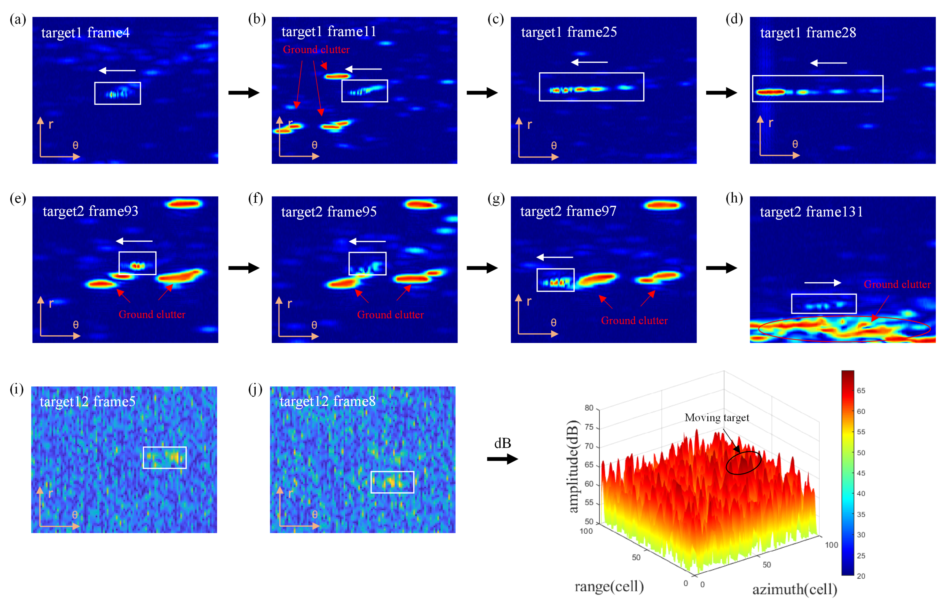
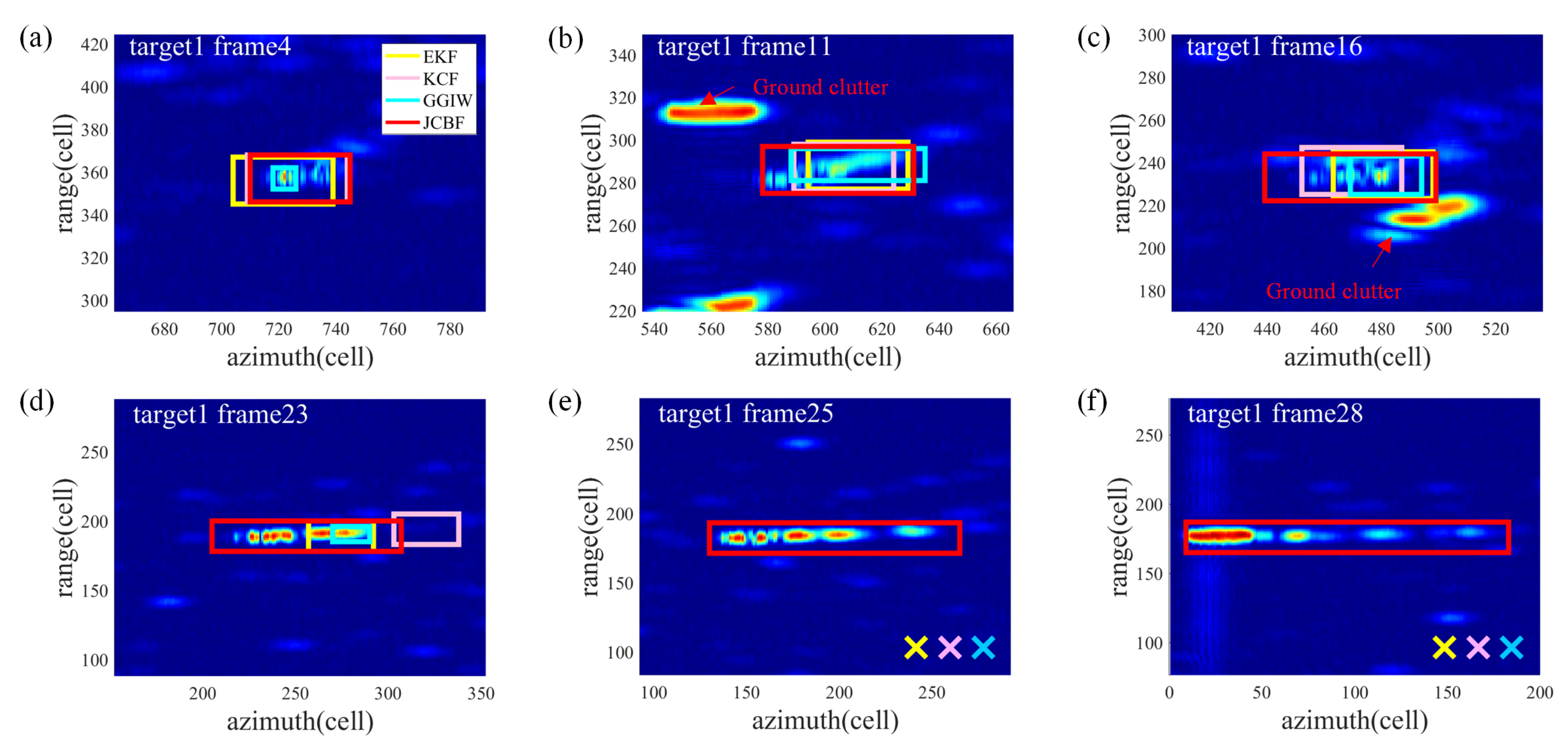
The experiments in this paper are performed using the data matrices of radar echoes. The proposed JCBF and several selected trackers are used to track each target separately. The results of each tracker are the center location and the bounding box of the targets. The targets in the radar monitoring scenario are non-cooperative, so the real motion information and the real labels of the targets can’t be obtained. In addition, the experimental results are compared with the manually generated labels to evaluate the trackers’ performance.

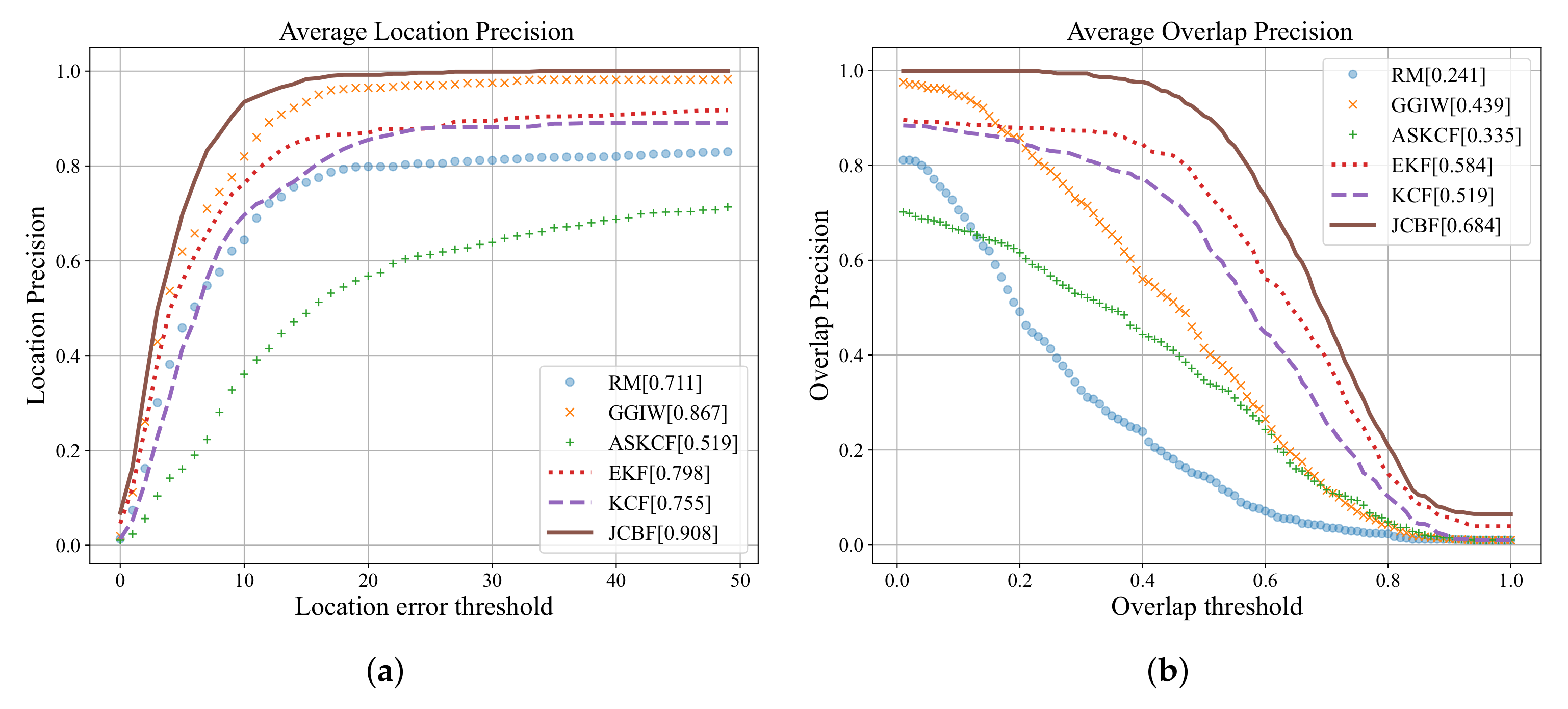
Average center location error (CLE) and bounding box overlap ratio are calculated to evaluate the difference between the results and the ground truth. For the performance criteria, the precision curves widely applied in the visual tracking [20,23,28] are also utilized to simply show the percentage of correctly tracked frames. Targets are considered to be tracked correctly if the predicted target center is within a distance threshold of ground truth.

The location precision and overlap precision are given by (35) and (36), respectively:

$$LP(\mathcal{G},\mathcal{T},t{h}_{lp})=\frac{sum(dist(\mathcal{G},\mathcal{T})\le t{h}_{lp})}{len\left(\mathcal{G}\right)},$$

(35)

$$OP(\mathcal{G},\mathcal{T},t{h}_{op})=\frac{sum(overlap(\mathcal{G},\mathcal{T})\ge t{h}_{op})}{len\left(\mathcal{G}\right)},$$

(36)

where $\mathcal{G}$ and $\mathcal{T}$ denote ground truth set and tracking results set, respectively. $dist(·)$ calculates the distance between the center of ground truth and the center of tracking results, and $overlap(·)$ calculates the intersection-over-union (IOU) between the ground truth and the tracking results. $t{h}_{lp}\in [0,50]$ and $t{h}_{op}\in [0,1]$ denote the location error threshold and overlap threshold, respectively.

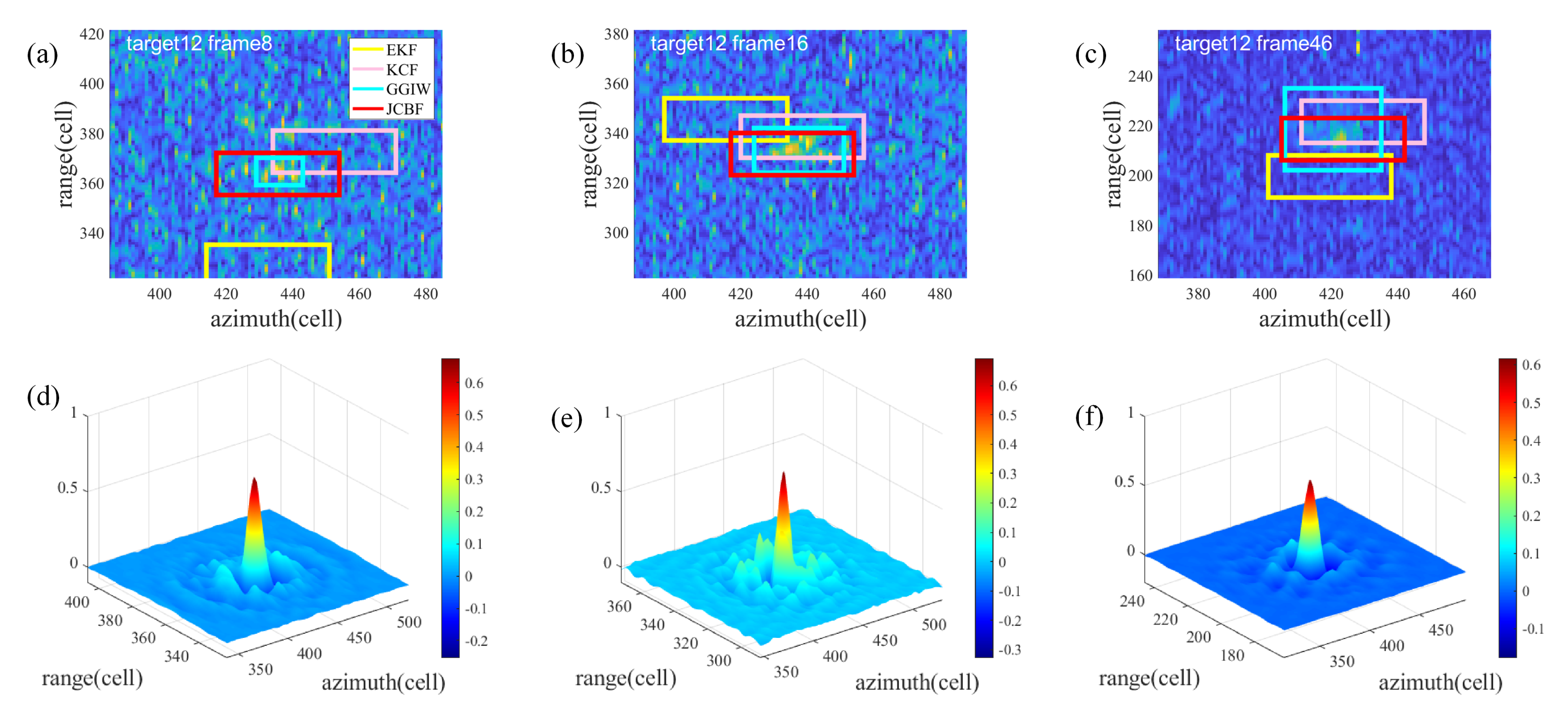
Three traditional Bayes tracking methods (EKF [2], RM-based trackers [5], GGIW-based trackers [9]) and two correlation filter-based methods (KCF [20], Scale Adaptive with Multiple Features tracker (ASKCF) [21]) are chosen to compare with JCBF. The same measurements are provided for three Bayes methods and the proposed JCBF. In addition, the parameters of the two correlation filters are the same as those of the proposed JCBF.

It is worth noting that KF has been used for smoothing the measurements in both RM-based trackers and GGIW-based trackers, the KF parameters of the two trackers are the same as those of JCBF. To show the performance improvement of the JCBF, the EKF supplemented by the nearest neighbor data correlation is also tested on the same dataset. Furthermore, the IOU is calculated based on the target size on the first frame, as the EKF cannot estimate the size of targets based on the point target hypothesis.

3. Experiment and Results Analysis

3.1. Data Sets Analysis

Experimental data sets were provided by Naval Aviation University [29,30] and collected on 22 July 2020. Overall, 136 frames of scanning data were collected by an X-band marine radar near the Yantai harbor, Yantai, China. The radar scan speed is 24 rpm and emits rectangular pulses with a PRF of 1.6 kHz. A frame of the radar image in the original data is formatted with 2224 cells in range and 1729 cells in azimuth. The detailed parameters of the experimental radar are displayed in

Table 3. X-band experimental radar parameters.

Parameter	Value
Operating Frequency	9.3–9.5 GHz
Output Power	50 W
Antenna Beamwidth	1.2 deg @ −3 dB
Rate of Rotation	24 rpm
Number of Range Samples	1729
Number of Azimuth Samples	2224
Range Resolution Cell	6 m
Azimuth Resolution Cell	360°/5120

.

Moreover, some of the azimuth cell data in the original data are duplicated or missing, thus the data need to be corrected, and the size of the corrected data is 2224 × 2078 (range cells × azimuth cells).

There are twelve targets in the monitoring scene, whose manually labeled real trajectories are shown in Figure 3. The radar is interfered by some unknown objects during the scanning process, resulting in the blocking of the 571st to 716th azimuth cells, which are marked by the white dotted boxes in Figure 3. The trajectories of the targets passing through this area are divided into two segments because there is no useful information in the radar echoes of the targets as they pass through these areas, e.g., target 1 (target 9) and target 6 (target 10).

3.2. Performance Analysis

The tracking trajectories of twelve targets from the proposed method are shown in Figure Figure 4.

3.2.1. Time Costing

Above experiments are performed on a workstation with the i5-10500 3.10 GHz CPU and 24 GB RAM. The costing time per target per frame is recorded in

Table 4. Cost time per frame.

Methods	RM	GGIW	ASKCF	EKF	KCF	JCBF
Cost time	0.027	0.029	0.223	0.018	0.167	0.275

. For every target, the proposed method costs 0.275 s per frame, which costs more time than others for the reason that two filters are utilized in JCBF.

3.2.2. Error and Precision

Table 5. Center location error (CLE ↓, ↓ means lower is better).

Targets	RM	GGIW	ASKCF	EKF	KCF	JCBF
target1	11.9	34.3	7.8	34.5	32.7	7.3
target2	23.6	17.4	21.5	30.3	145.0	4.8
target3	235.4	2.3	300.0	2.3	2.0	1.8
target4	6.6	6.5	26.6	6.5	16.5	4.3
target5	36.3	5.9	10.5	33.8	46.4	4.0
target6	5.6	5.9	7.9	7.3	6.0	4.2
target7	2.6	2.6	9.6	5.2	5.6	2.6
target8	6.8	6.8	32.9	5.9	4.5	5.9
target9	4.1	4.3	318.2	3.8	3.3	4.2
target10	5.4	5.6	12.8	5.6	5.1	5.2
target11	88.9	2.4	267.7	61.9	30.1	2.0
target12	44.1	3.1	296.8	6.5	12.5	3.5
Average	39.3	8.7	109.4	16.7	25.8	4.1

,

Table 6. Average location precision (LP ∈ [0, 1] ↑, ↑ means higher is better).

Targets	RM	GGIW	ASKCF	EKF	KCF	JCBF
target1	0.750	0.648	0.834	0.645	0.688	0.844
target2	0.773	0.768	0.681	0.727	0.330	0.895
target3	0.106	0.944	0.177	0.943	0.948	0.954
target4	0.858	0.860	0.459	0.861	0.716	0.905
target5	0.629	0.871	0.778	0.664	0.538	0.910
target6	0.879	0.873	0.831	0.879	0.871	0.908
target7	0.938	0.939	0.798	0.888	0.876	0.939
target8	0.852	0.853	0.519	0.897	0.899	0.875
target9	0.910	0.904	0.053	0.912	0.924	0.911
target10	0.883	0.877	0.733	0.880	0.886	0.888
target11	0.390	0.941	0.125	0.424	0.648	0.951
target12	0.569	0.928	0.243	0.861	0.739	0.919
Average	0.711	0.867	0.519	0.798	0.755	0.908

and

Table 7. Average overlap precision (OP [0, 1] ∈ ↑, ↑ means higher is better).

Targets	RM	GGIW	ASKCF	EKF	KCF	JCBF
target1	0.227	0.271	0.603	0.449	0.473	0.653
target2	0.210	0.326	0.331	0.469	0.192	0.635
target3	0.048	0.618	0.105	0.776	0.785	0.774
target4	0.443	0.504	0.312	0.606	0.534	0.647
target5	0.291	0.463	0.514	0.504	0.350	0.700
target6	0.374	0.407	0.597	0.666	0.581	0.687
target7	0.322	0.519	0.519	0.637	0.562	0.681
target8	0.320	0.359	0.253	0.618	0.605	0.621
target9	0.160	0.404	0.040	0.668	0.686	0.672
target10	0.245	0.299	0.530	0.687	0.704	0.722
target11	0.100	0.570	0.073	0.317	0.433	0.751
target12	0.159	0.534	0.149	0.591	0.326	0.670
Average	0.241	0.439	0.335	0.584	0.519	0.684

compare the center location error, location precision and overlap precision of the results obtained from six trackers, respectively. Additionally, the average location precision curves and average overlap precision curves are displayed in Figure 5a,b, respectively, which present the results more visually. The larger values of the location precision and the overlap precision mean the more accurate result.

As can be seen from Table 5 and Table 6, the proposed JCBF with the lowest average location error and highest average location precision can accurately capture the center of the target. It can be seen from the results in Figure 5 and Table 6Table 7 that the proposed method performs better than others in estimating the size of the target.

GGIW and RM are easy to misclassify measurements when the shape of the target changes or the target is disturbed by clutter. In addition, the scaling pool used by ASKCF is not suitable for radar targets as discussed in Section 2.5.2, which results in location and shape estimation errors. Moreover, the scaling pool used in ASKCF is easier to introduce the clutter into the sampling area. Furthermore, the difference between the target and clutter is most reflected in the phase of radar’s echo, but not the amplitude of the radar’s echo. Therefore, the clutter is easy to be regarded as the target by ASKCF, which will lead to the decline in the performance. Therefore, ASKCF is not suitable for radar targets. It’s noting that although the $OP$ of KCF and EKF is shown to demonstrate the performance improvement of the JCBF relative to them, it does not mean that they have the ability to estimate the size of targets.

Comparing the above results, it can be seen that the proposed JCBF has the significantly improved performance over other tracking algorithms. The reason is that the proposed JCBF exploits both the motion and appearance features of the target, which improves the algorithm’s ability to distinguish between targets and clutter. Moreover, the feedback strategy improves the stability of the trackers and the proposed scaling pool is more suitable for radar targets.

3.3. Tracking Results Analysis

Table 8. Some challenging targets in monitor scenarios.

Challenging Situations	Targets
Shape or appearance changing	target1, target4, target5
Multiple scattering points	target1, target4, target5
Interferenced by clutter	target1, target2, target3
Weak target	target12
Maneuvering targets	target1, target2

lists the challenging situations in the date sets. Some typical targets can be seen in Figure 6 are selected to visually show these situations, where the white boxes in figures indicate the position of the target and the white arrows indicate the direction of the target movement. When the maritime radar is working at scanning mode, target 1 produces different azimuthal expansion at each time due to radar’s beam width, as shown in Figure 6a–d. Target 2 is obscured (see Figure 6e–g) or interfered with (see Figure 6h) by ground clutter. Furthermore, target 12 is a weak target with low SNR at most frames, whose SNR is statistically 7.3 dB. The top four best performing algorithms (JCBF, EKF, KCF, GGIW) in Section 3.2 are selected for detailed analysis.

3.3.1. Shape or Appearance Changing

Figure 7 shows the tracking bounding boxes of target 1 given by JCBF and those of others in some key frames, where red boxes denote the JCBF, pink boxes denote the KCF, yellow boxes denote the EKF, and blue boxes denote the GGIW. Missing trackers are denoted by an ’×’.

Due to azimuthal scaling, the target tends to produce multiple measurements, which can easily lead to association errors during tracking. It can be seen from the results in Figure 7 that EKF estimates the position of the target incorrectly and gradually loses it when the target’s shape changes, because EKF only selects the measurement closest to the prediction. In addition, the measurements are so dispersed in azimuth, which causes the GGIW clusters incorrectly. KCF tracks reasonably well in the first few frames when target scales not obviously, but loses the target in both Figure 7e,f because the template size cannot change with the scaling of the target. In comparison, the proposed JCBF can capture the changing of the target’s size precisely.

In order to illustrate the advantages of the proposed algorithm in dealing with targets’ deformation more directly, the response maps of KCF and JCBF at frame 23 are compared in Figure 8. It can be seen that the response map of KCF fluctuates intensely because the target has multiple strong scattering points, while that of JCBF has high-confidence due to the high PSR.

3.3.2. Targets Interferenced by Clutter

Figure 9a–c compare the results of target 2 given by all trackers when the target is briefly obscured by clutter. Figure 9d–f show the results of target 2 under the circumstance that it approaches land at high speed and is interferenced by ground clutter.

It is seen from Figure 10 that the false sharp peak of the response map of KCF is within the clutter region, because the target is obscured by a stationary clutter from frame 94 to frame 96, which results in an incorrect position of KCF, as shown in Figure 9b,c. However, the target’s motion model is not affected by the clutter and when the target reappeared, the EKF module in the proposed JCBF can correctly track the target using real-time measurements, as shown in Figure 9c.

After frame 120, target 2 maneuvers closer to land and swerves quickly, whose motion model is not conforming to the preset uniform linear motion model and measurements are interferenced by clutter. It causes the wrong association and results in traditional trackers (EKF, GGIW) drifting, as shown in Figure 9d–f. However, response maps with high confidence are still obtained in JCBF, as the appearance of the target remains intact, as shown in Figure 11. As a result, the proposed JCBF is precise on locating the centroid of the target.

3.3.3. Weak Targets

Figure 12a–c give the results of target 12 given by all trackers. Under a low signal-to-clutter/noise ratio (SCR/SNR) environment, the existing detectors have poor detection performance and cannot provide effective measurements for trackers, which results in tracking errors of traditional tracking-by-detection tracker (EKF, GGIW). As Figure 12 shown, EKF is prone to produce location errors and GGIW incorrectly estimates the target’s size due to the obtained valid measurements. However, as displayed in Figure 12d–f, the JCBF is still able to accurately capture target 12 because of the high-confidence responses of the KCF module. Moreover, the feedback strategy continuously feeds repositioned high-confidence measurements and samples to the EKF and KCF modules, which improves the stability of the proposed JCBF at low SNR.

According to the above analysis, the performance of the JCBF is significantly better than the traditional methods since both the appearance information and the motion information of the target are utilized.

4. Discussion

4.1. Associations with Previous Research

Traditional radar target tracking algorithms rely on temporal evolution models and observation models, using the accumulated detector measurement as input with the aim of iteratively calculating the posterior PDF of the target’s kinematic state. These techniques can be described within unified Bayesian formalism [4]. With the improvement of modern radar resolution, the extended characteristics of targets have received more attention, while a number of extended target tracking algorithms within the Bayes framework have been proposed [5].

In the field of visual target tracking, the specificity of the target’s appearance features make it important for specific target discrimination. At the same time, the complexity of appearance features also make them intractable to model statistically, leading to a range of data-driven learning-based algorithms [18,20]. These algorithms allow for the efficient extraction and characterization of the target’s appearance information, but also directly lead to the representation of the appearance features being hard to include in the unified Bayesian formalism.

This paper proposes a method that incorporates the output of CF into a BF formalism, thus providing a scheme combining the appearance information extracted by learning-based algorithms with the motion information of the target, which is derived from the idea of regarding the output of the CF as a PDF of the target position in [23]. Through this, the proposed method would combine the specificity of the appearance representation provided by learning-based algorithms with the memorability of motion properties offered by Bayesian approach. The experimental results demonstrate the effectiveness of the proposed method, which has significant advantages over the traditional BF and CF in scenarios of clutter interference, target’s shape changing, and low SNR.

Based on the unity of the Bayesian formalism, it is reasonable to believe that most tracking algorithms which can be described within Bayesian formalism have the potential to be combined with CF using the method proposed in this paper.

4.2. Suggestions for Future Work

On the one hand, the CF relies on labeled data for initialization, which makes the proposed method’s automatic initiation become problematic. It is essential to address the tracker’s automatic initiation. On the other hand, the combination of other data-driven algorithms with Bayesian formalism and the extension of this method to multi-target scenarios are also subject to further research.

5. Conclusions

This paper proposes a new tracking framework based on correlation filter and Bayes filter for marine radar single-target tracking. The proposed JCBF is able to track the motion state and appearance of the target simultaneously by fusing the correlation filter and Bayes filter. Taking into account more available information of the radar target, the proposed method maintains robustness in the complex environment. The feedback structure improves the tracker’s stability and the scale adaptive strategy enables the tracker to adapt to the targets’ shape changing. Experiments on X-band marine radar data demonstrate that the JCBF performs better than traditional methods in some complex situations such as clutter interference, target’s shape changing, and low SNR. The experiments also indicate that statistical learning methods like KCF have the potential to be used widely in radar target tracking.

There is still some room for improvement of multi-target tracking in the proposed method. Further, a JCBF-based multi-target tracking framework will be investigated in depth.

References

1. Kalman, R.E. A new approach to linear filtering and prediction problems. Trans. ASME 1960, 1, 35–45. [Google Scholar] [CrossRef] [Green Version]
2. Daeipour, E.; Bar-Shalom, Y. An interacting multiple model approach for target tracking with glint noise. IEEE Trans. Aerosp. Electron. Syst. 1995, 31, 706–715. [Google Scholar] [CrossRef]
3. Julier, S.J.; Jeffrey, K.U.; Hugh, F.D. A new approach for filtering nonlinear systems. In Proceedings of the IEEE 1995 American Control Conference, Seattle, WA, USA, 21–23 June 1995; Volume 3. [Google Scholar]
4. Mahler, R.P.S. Advances in Statistical Multisource-Multitarget Information Fusion; Artech House: London, UK, 2014. [Google Scholar]
5. Koch, J.W. Bayesian approach to extended object and cluster tracking using random matrices. IEEE Trans. Aerosp. Electron. Syst. 2008, 44, 1042–1059. [Google Scholar]
6. Feldmann, M.; Fränken, D.; Koch, W. Tracking of Extended Objects and Group Targets Using Random Matrices. IEEE Trans. Signal Process. 2011, 59, 1409–1420. [Google Scholar] [CrossRef]
7. Orguner, U. A Variational Measurement Update for Extended Target Tracking with Random Matrices. IEEE Trans. Signal Process. 2012, 60, 3827–3834. [Google Scholar] [CrossRef]
8. Granstrom, K.; Orguner, U. A phd Filter for Tracking Multiple Extended Targets Using Random Matrices. IEEE Trans. Signal Process. 2012, 60, 5657–5671. [Google Scholar] [CrossRef] [Green Version]
9. Granström, K.; Natale, A.; Braca, P.; Ludeno, G.; Serafino, F. Gamma Gaussian Inverse Wishart Probability Hypothesis Density for Extended Target Tracking Using X-Band Marine Radar Data. IEEE Trans. Geosci. Remote Sens. 2015, 53, 6617–6631. [Google Scholar]
10. Marcus, B.; Uwe, D.H. Extended Object Tracking with Random Hypersurface Models. IEEE Trans. Aerosp. Electron. Syst. 2014, 50, 149–159. [Google Scholar]
11. Antonio, Z.; Florian, F.; Marcus, B.; Uwe, D.H. Level-set random hypersurface models for tracking nonconvex extended objects. IEEE Trans. Aerosp. Electron. Syst. 2016, 52, 2990–3007. [Google Scholar]
12. Niklas, W.; Emre, O. Extended Target Tracking Using Gaussian Processes. IEEE Trans. Signal Process. 2015, 63, 4165–4178. [Google Scholar]
13. Shui, P.L.; Li, C.D.; Xu, S.W. Tri-feature-based detection of floating small targets in sea clutter. IEEE Trans. Aerosp. Electron. Syst. 2014, 50, 1416–1430. [Google Scholar] [CrossRef]
14. Sun, J.P.; Liu, C.; Li, Q.; Chen, X.L. Labeled multi-bernoulli filter with amplitude information for tracking marine weak targets. IET Radar Sonar Navig. 2019, 13, 983–991. [Google Scholar] [CrossRef]
15. Kim, D.; Hwang, I. Dynamic model-based feature aided data association filter in target tracking. IET Radar Sonar Navig. 2019, 14, 279–289. [Google Scholar] [CrossRef]
16. Zhu, Y.P.; Wang, Z.; Yin, Y.P.; Chen, W.D. Feature-aided Multi-Target Tracking Method in Sea Clutter Using Scanning Radar Data. In Proceedings of the 2021 IEEE 6th International Conference on Signal and Image Processing (ICSIP), Nanjing, China, 9–11 July 2021; pp. 615–619. [Google Scholar]
17. Yin, Y.P.; Cheng, D.; Dai, Y.L.; Chen, C.; Chen, W.D. Feature-aided GM-PHD Algorithm for Sea-surface Target Tracking. In Proceedings of the 2020 IEEE 5th International Conference on Signal and Image Processing (ICSIP), Nanjing, China, 3–5 July 2020; pp. 220–225. [Google Scholar]
18. Chen, X.L.; Su, N.Y.; Huang, Y.; Guan, J. False-Alarm-Controllable Radar Detection for Marine Target Based on Multi Features Fusion via CNNs. IEEE Sens. J. 2021, 21, 9099–9111. [Google Scholar]
19. Su, N.Y.; Chen, X.L.; Guan, J.; Huang, Y. Maritime Target Detection Based on Radar Graph Data and Graph Convolutional Network. IEEE Geosci. Remote Sens. Lett. 2022, 19, 1–5. [Google Scholar] [CrossRef]
20. Henriques, J.F.; Caseiro, R.; Martins, P.; Batista, J. High-Speed Tracking with Kernelized Correlation Filters. IEEE Trans. Pattern Anal. Mach. Intell. 2015, 37, 583–596. [Google Scholar]
21. Danelljan, M.; Hager, G.; Khan, F.S.; Felsberg, M. Accurate scale estimation for robust visual tracking. In Proceedings of the British MachineVision Conference, Nottingham, UK, 1–5 September 2014; BMVA Press: Durham, UK, 2014. [Google Scholar]
22. Li, Y.; Zhu, J. A scale adaptive kernel correlation filter tracker with feature integration. In Proceedings of the European Conference on Computer Vision, Cham, Switzerland, 6–12 September 2014; pp. 254–265. [Google Scholar]
23. Zhou, Y.; Wang, T.; Hu, R.H.; Su, H. Multiple Kernelized Correlation Filters (MKCF) for Extended Object Tracking Using X-Band Marine Radar Data. IEEE Trans. Signal Process. 2019, 67, 3676–3688. [Google Scholar]
24. Mehmood, K.; Jalil, A.; Ali, A.; Khan, B.; Murad, M.; Khan, W.U.; He, Y. Context-aware and occlusion handling mechanism for online visual object tracking. Electronics 2020, 10, 43. [Google Scholar] [CrossRef]
25. Yu, C.L.; Zhan, R.H.; Wan, J.W. Research on Robust UKF Algorithm for Single Observer Passive Target Tracking Based on Polar Coordinates. J. Nat. Univ. Def. Technol. 2008, 30, 7. [Google Scholar]
26. Bolme, D.S.; Beveridge, J.R.; Draper, B.A.; Lui, Y.M. Visual object tracking using adaptive correlation filters. In Proceedings of the 2010 IEEE Computer Society Conference on Computer Vision and Pattern Recognition, San Francisco, CA, USA, 13–18 June 2010; pp. 2544–2550. [Google Scholar]
27. Wang, M.M.; Liu, Y.; Huang, Z.Y. Large Margin Object Tracking with Circulant Feature Maps. In Proceedings of the 2017 IEEE Conference on Computer Vision and Pattern Recognition (CVPR), Honolulu, HI, USA, 21–26 July 2017; pp. 4800–4808. [Google Scholar]
28. Babenko, B.; Yang, M.; Belongie, S. Robust Object Tracking with Online Multiple Instance Learning. IEEE Trans. Pattern Anal. Mach. Intell. 2011, 33, 1619–1632. [Google Scholar]
29. Liu, N.B.; Ding, H.; Huang, Y. Annual Progress of Sea-detecting X-band Radar and Data Acquisition Program. J. Radars 2021, 10, 173–182. [Google Scholar]
30. Liu, N.B.; Yunlong, D.; Wang, G.Q. Sea-detecting X-band radar and data acquisition program. J. Radars 2019, 8, 656–667. [Google Scholar]
31. Roecker, J.A.; McGillem, C.D. Target tracking in maneuver centered coordinates. In Proceedings of the 1988 IEEE National Radar Conference, Ann Arbor, MI, USA, 20–21 April 1988; pp. 68–73. [Google Scholar]
Figure 1. Overall flow of the proposed method. (a) Bayes filter module. (b) Correlation filter module. (c) Fusion module. The green lines indicate the feedback for correcting measurements. Both the process of providing measurements for Kalman filter by detector and the training process of the correlation filter are omitted in the figure.
Remotesensing 14 05937 g001
Figure 2. Common challenging situations. (a) Appearance changing. (b) Interruption measurements.
Remotesensing 14 05937 g002
Figure 3. Twelve trajectories of moving targets by manually labeled.
Remotesensing 14 05937 g003
Figure 4. The tracking results of the proposed JCBF.
Remotesensing 14 05937 g004
Figure 5. Average location precision and overlap precision of twelve targets. (a) Average location precision curves (DP ∈ [0, 1]) of twelve targets. (b) Average overlap precision curves (OP ∈ [0, 1]) of twelve targets.
Remotesensing 14 05937 g005
Figure 6. Some challenging targets in monitor scenarios. (ad) Shape or appearance changing. (eh) Targets interferenced by clutter. (i,j) Weak targets.
Remotesensing 14 05937 g006
Figure 7. Tracking results of target 1 at some key frames. (af): Tracking results for each filter when the shape of target 1 changes.
Remotesensing 14 05937 g007
Figure 8. The response maps of (a) KCF and (b) JCBF (target 1 in frame 23).
Remotesensing 14 05937 g008
Figure 9. Tracking results of target 2 at some key frames. (af) Tracking results for each filter when target 2 is obscured by clutter.
Remotesensing 14 05937 g009
Figure 10. The response maps of KCF (target 2 in frame 95 and frame 96). (a) The response maps in frame 95. (b) The response maps in frame 96.
Remotesensing 14 05937 g010
Figure 11. The response map of JCBF (target 2 in frame 131).
Remotesensing 14 05937 g011
Figure 12. Tracking results of target 12 at some key frames. (ac) The rusults of four trackers. (df) The responses of the proposed JCBF.
Remotesensing 14 05937 g012