
Evaluation of the Use of UAV-Derived Vegetation Indices and Environmental Variables for Grapevine Water Status Monitoring Based on Machine Learning Algorithms and SHAP Analysis


Abstract

1. Introduction
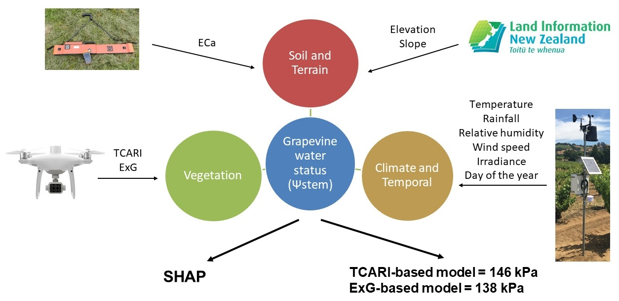
2. Materials and Methods
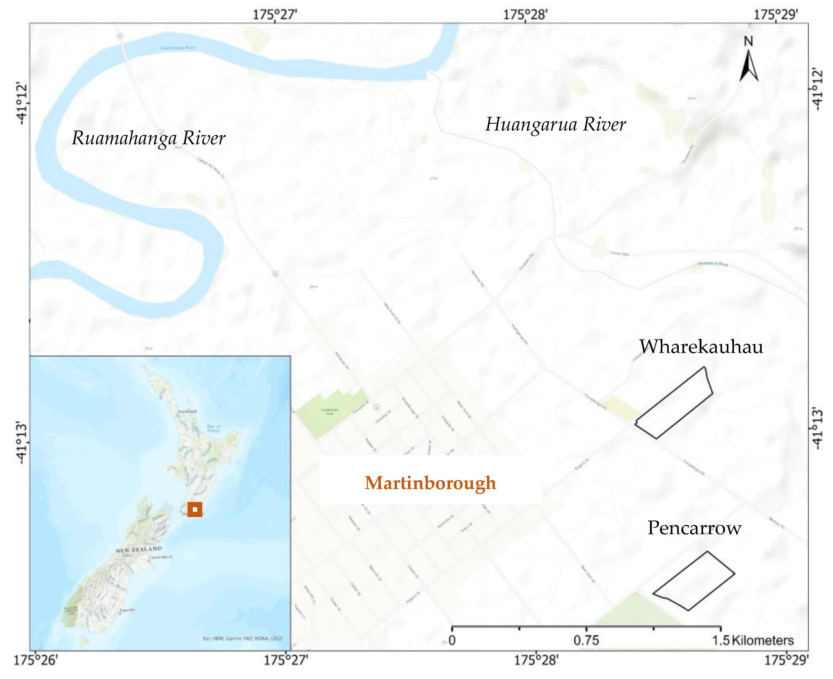
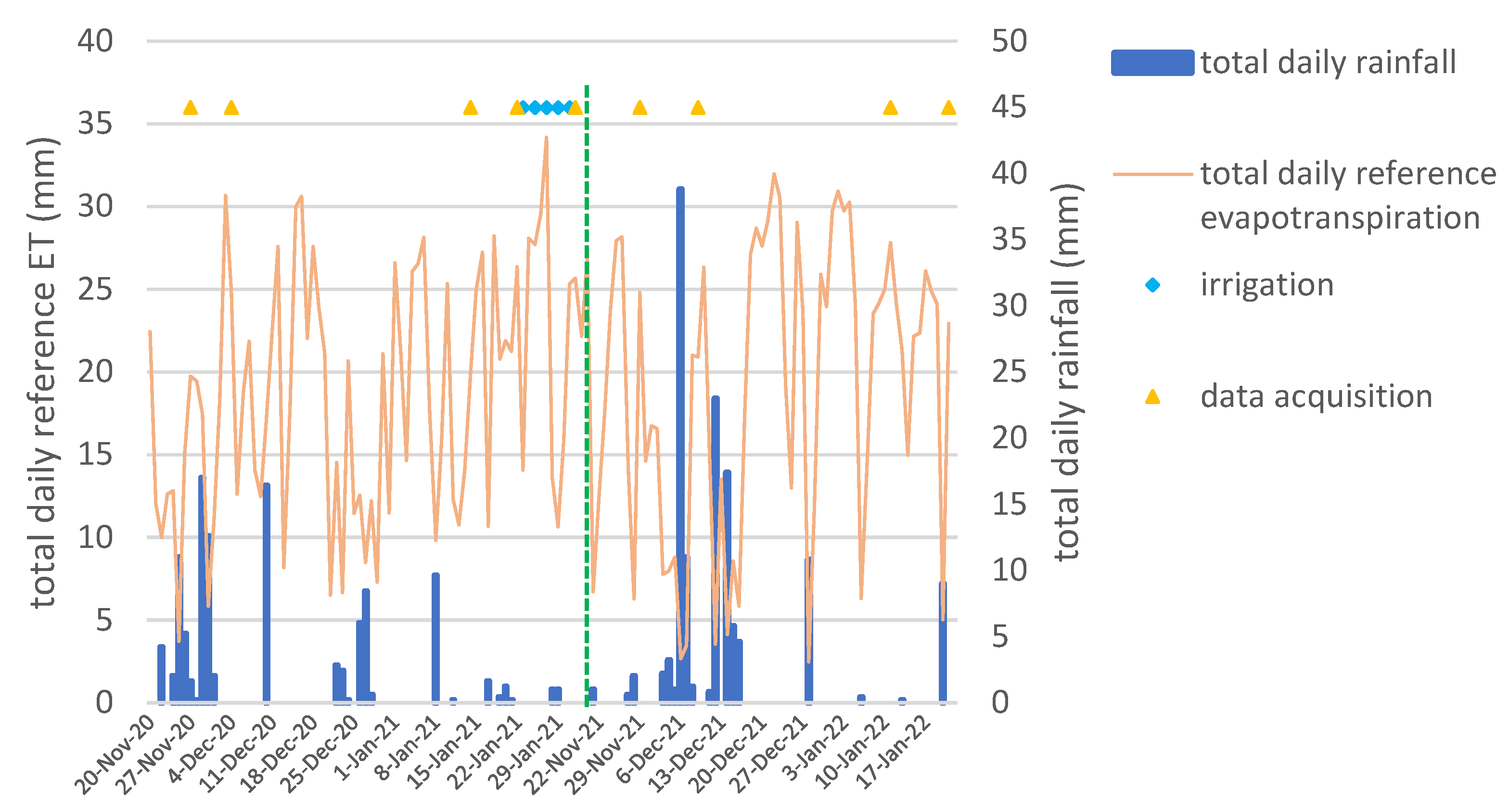
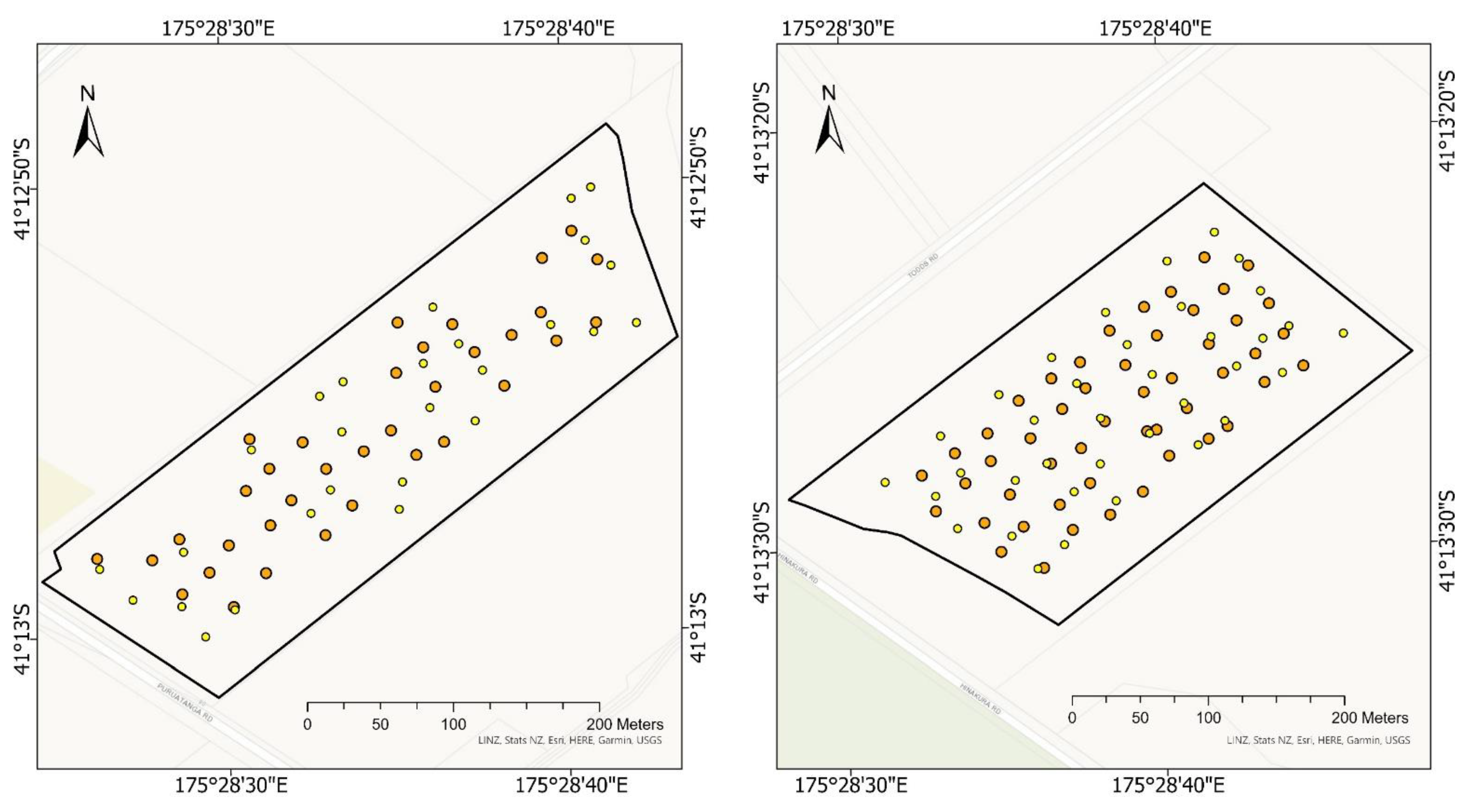
2.1. The Context of the Study Vineyards and Study Periods
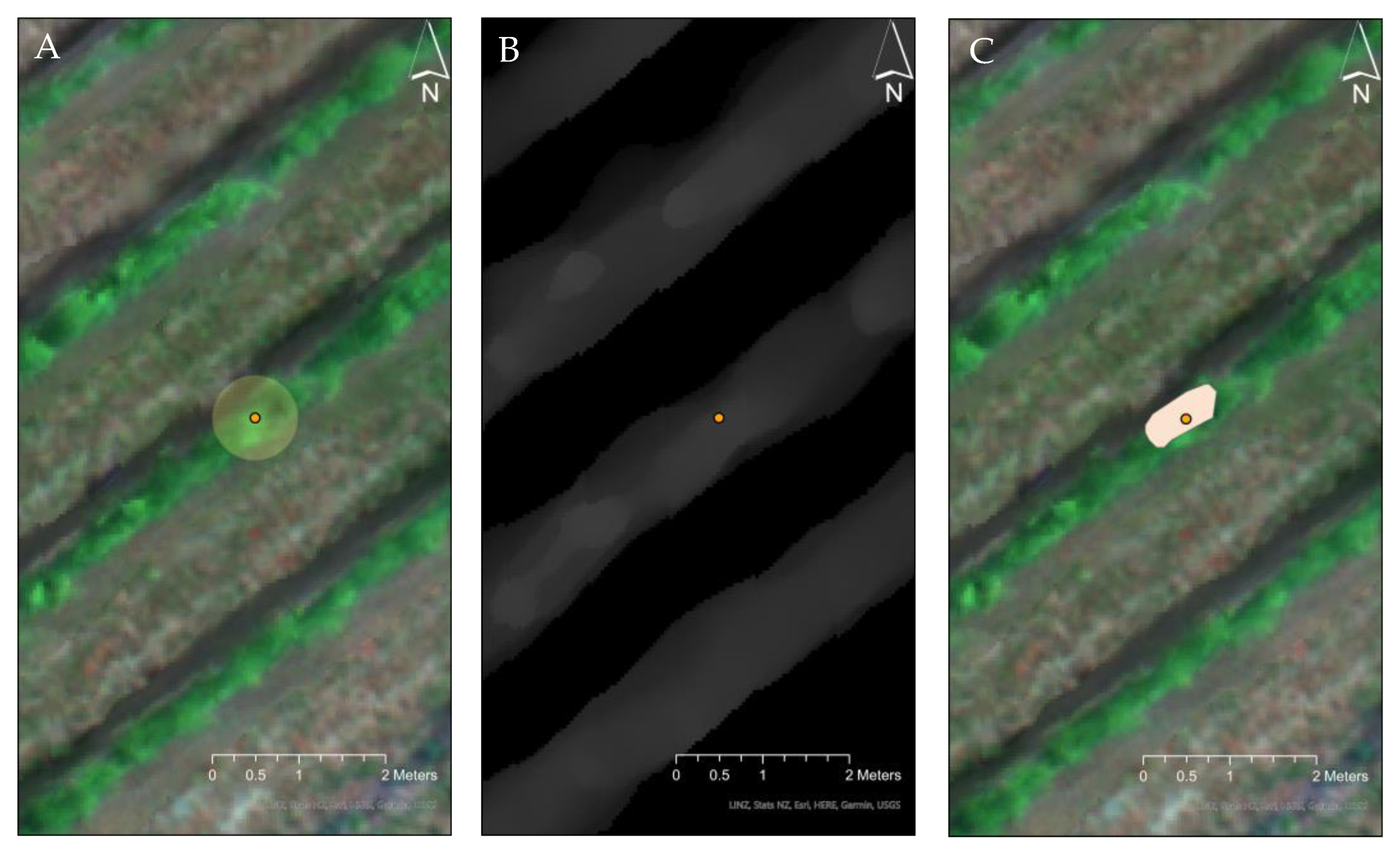
2.2. Response Variable-Stem Water Potential
2.3. Predictor Variable-Vegetation Parameters
2.4. Predictor Variable-Soil and Terrain Information
2.5. Predictor Variable-Meteorological and Temporal Data
2.6. Hierarchical Clustering
2.7. Regression Modeling
2.8. Shapley Additive Explanations Analysis
3. Results
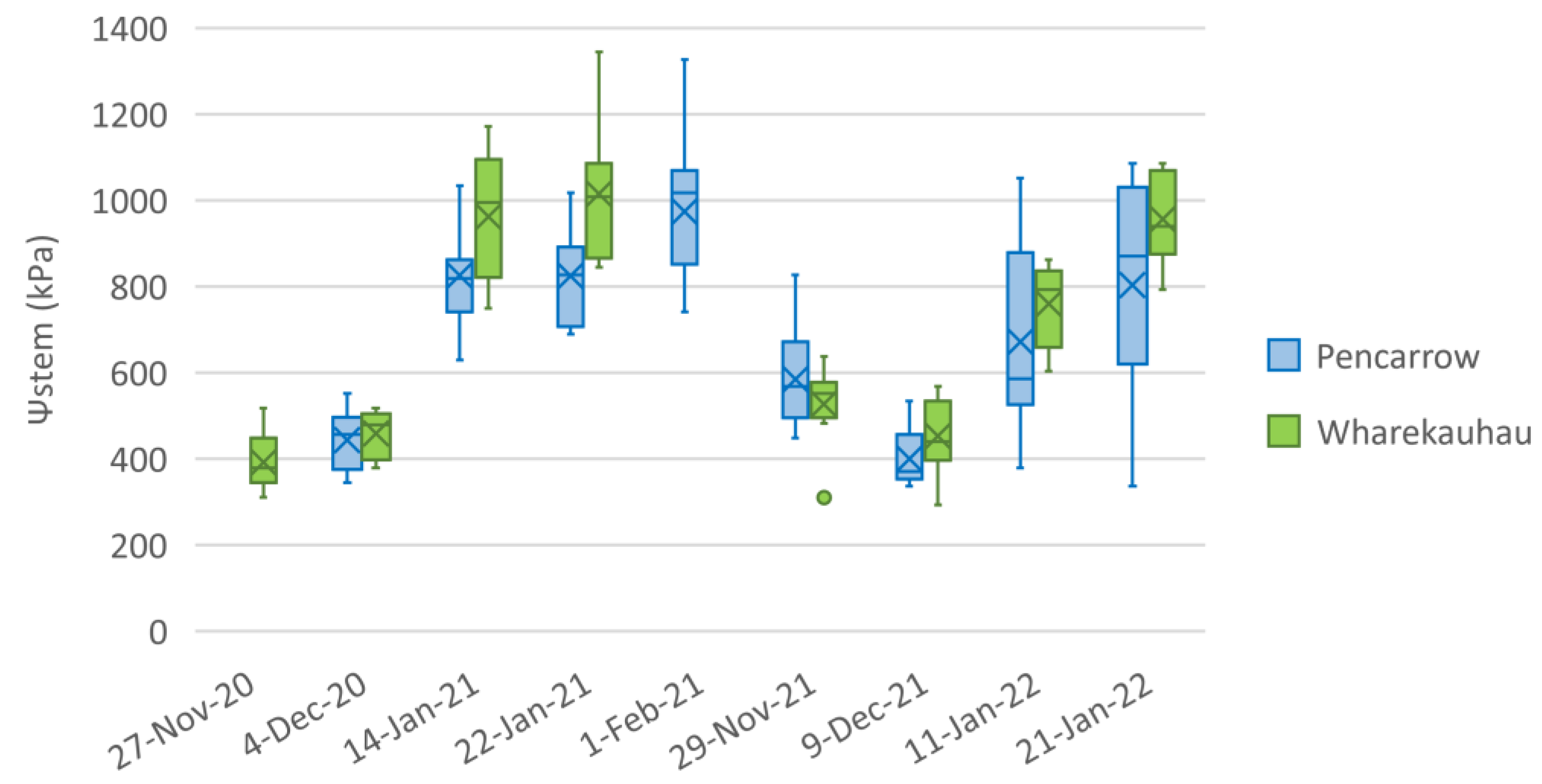
3.1. Variation in Stem Water Potential
3.2. Determination of the Best Descriptor of Vegetation Index for Variation in Grapevine Water Status
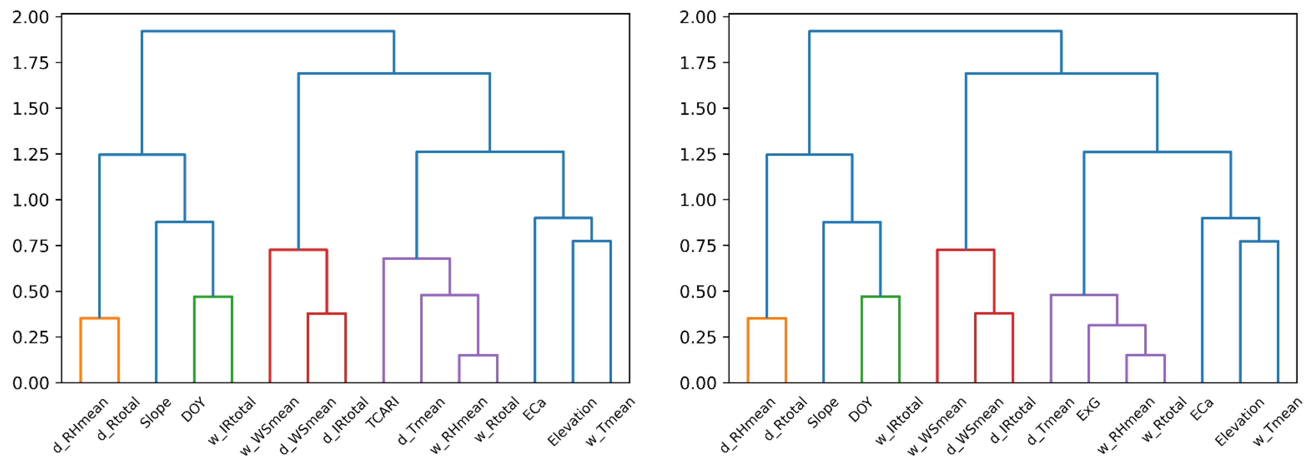
3.3. Selection of Predictor Variables as Inputs for Modeling Using Hierarchical Clustering
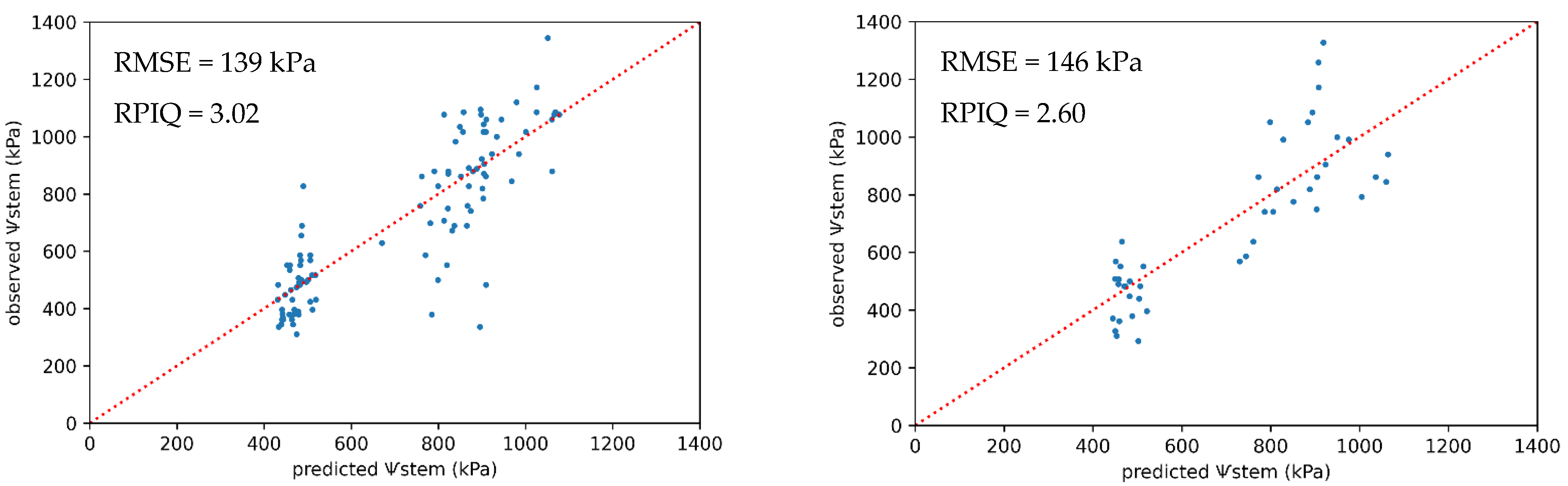
3.4. Regression of Grapevine Water Status Based on Core and Ancillary Variables
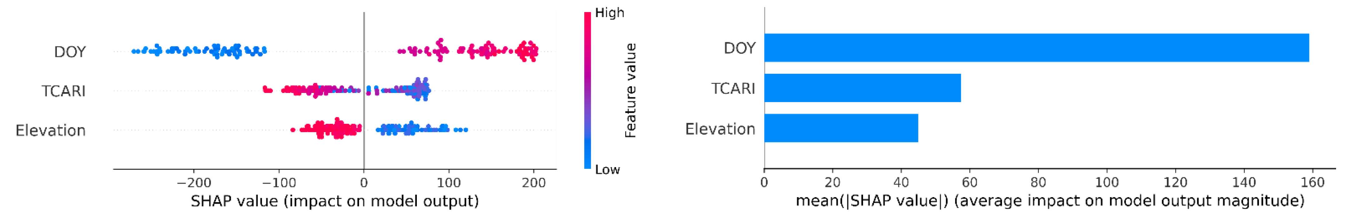
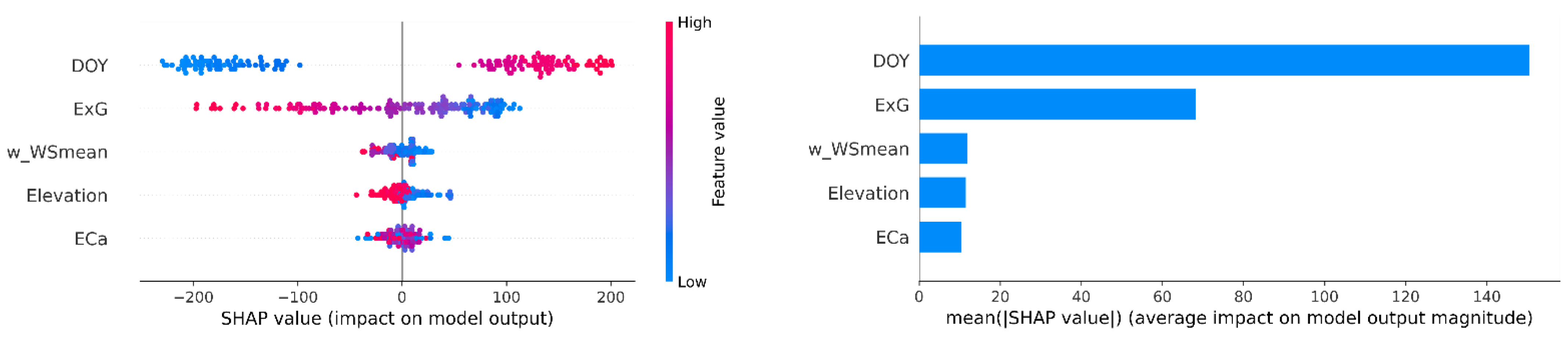
3.5. Interpreting Models Using Shapley Additive exPlanations Analysis
4. Discussion
4.1. Vegetation Indices and Stem Water Potential
4.2. Important Ancillary Variables: Day of the Year, Elevation, Electrical Conductivity, and Wind Speed
4.3. Regression Modeling
4.4. Limitations and Future Work
5. Conclusions
Author Contributions
Funding
Data Availability Statement
Acknowledgments
Conflicts of Interest
References
- Ojeda, H.; Andary, C.; Kraeva, E.; Carbonneau, A.; Deloire, A. Influence of pre-and postveraison water deficit on synthesis and concentration of skin phenolic compounds during berry growth of Vitis vinifera cv. Shiraz. Am. J. Enol. Vitic. 2002, 53, 261–267. [Google Scholar]
- Martínez-Lüscher, J.; Sánchez-Díaz, M.; Delrot, S.; Aguirreolea, J.; Pascual, I.; Gomes, E. Ultraviolet-B Radiation and Water Deficit Interact to Alter Flavonol and Anthocyanin Profiles in Grapevine Berries through Transcriptomic Regulation. Plant Cell Physiol. 2014, 55, 1925–1936. [Google Scholar] [CrossRef] [PubMed]
- Van Leeuwen, C.; Trégoat, O.; Choné, X.; Bois, B.; Pernet, D.; Gaudillère, J.-P. Vine water status is a key factor in grape ripening and vintage quality for red Bordeaux wine. How can it be assessed for vineyard management purposes? J. Int. Sci. Vigne Vin 2009, 43, 121–134. [Google Scholar] [CrossRef]
- Acevedo-Opazo, C.; Valdés-Gómez, H.; Taylor, J.; Avalo, A.; Verdugo-Vásquez, N.; Araya, M.; Jara-Rojas, F.; Tisseyre, B. Assessment of an empirical spatial prediction model of vine water status for irrigation management in a grapevine field. Agric. Water Manag. 2013, 124, 58–68. [Google Scholar] [CrossRef]
- Intrigliolo, D.S.; Castel, J.R. Response of grapevine cv. ‘Tempranillo’ to timing and amount of irrigation: Water relations, vine growth, yield and berry and wine composition. Irrig. Sci. 2009, 28, 113–125. [Google Scholar] [CrossRef]
- Etchebarne, F.; Ojeda, H.; Hunter, J. Leaf: Fruit ratio and vine water status effects on Grenache Noir (Vitis vinifera L.) berry composition: Water, sugar, organic acids and cations. S. Afr. J. Enol. Vitic. 2010, 31, 106–115. [Google Scholar]
- Min, Z.; Li, R.; Chen, L.; Zhang, Y.; Li, Z.; Liu, M.; Ju, Y.; Fang, Y. Alleviation of drought stress in grapevine by foliar-applied strigolactones. Plant Physiol. Biochem. 2019, 135, 99–110. [Google Scholar] [CrossRef]
- Brillante, L.; Martínez-Luscher, J.; Yu, R.; Plank, C.M.; Sanchez, L.; Bates, T.L.; Brenneman, C.; Oberholster, A.; Kurtural, S.K. Assessing Spatial Variability of Grape Skin Flavonoids at the Vineyard Scale Based on Plant Water Status Mapping. J. Agric. Food Chem. 2017, 65, 5255–5265. [Google Scholar] [CrossRef]
- López-García, P.; Intrigliolo, D.S.; Moreno, M.A.; Martínez-Moreno, A.; Ortega, J.F.; Pérez-Álvarez, E.P.; Ballesteros, R. Assessment of Vineyard Water Status by Multispectral and RGB Imagery Obtained from an Unmanned Aerial Vehicle. Am. J. Enol. Vitic. 2021, 72, 285–297. [Google Scholar] [CrossRef]
- Bramley, R.; Ouzman, J.; Boss, P. Variation in vine vigour, grape yield and vineyard soils and topography as indicators of variation in the chemical composition of grapes, wine and wine sensory attributes. Aust. J. Grape Wine Res. 2011, 17, 217–229. [Google Scholar] [CrossRef]
- Baciocco, K.A.; Davis, R.E.; Jones, G.V. Climate and Bordeaux wine quality: Identifying the key factors that differentiate vintages based on Consensus rankings. J. Wine Res. 2014, 25, 75–90. [Google Scholar] [CrossRef]
- Liu, C.; Sun, P.-S.; Liu, S.-R. A review of plant spectral reflectance response to water physiological changes. Chin. J. Plant Ecol. 2016, 40, 80. [Google Scholar]
- Bowyer, P.; Danson, F. Sensitivity of spectral reflectance to variation in live fuel moisture content at leaf and canopy level. Remote Sens. Environ. 2004, 92, 297–308. [Google Scholar] [CrossRef]
- Jang, G.; Kim, J.; Yu, J.-K.; Kim, H.-J.; Kim, Y.; Kim, D.-W.; Kim, K.-H.; Lee, C.W.; Chung, Y.S. Review: Cost-Effective Unmanned Aerial Vehicle (UAV) Platform for Field Plant Breeding Application. Remote Sens. 2020, 12, 998. [Google Scholar] [CrossRef]
- Rapaport, T.; Hochberg, U.; Shoshany, M.; Karnieli, A.; Rachmilevitch, S. Combining leaf physiology, hyperspectral imaging and partial least squares-regression (PLS-R) for grapevine water status assessment. ISPRS J. Photogramm. Remote Sens. 2015, 109, 88–97. [Google Scholar] [CrossRef]
- Brook, A.; De Micco, V.; Battipaglia, G.; Erbaggio, A.; Ludeno, G.; Catapano, I.; Bonfante, A. A smart multiple spatial and temporal resolution system to support precision agriculture from satellite images: Proof of concept on Aglianico vineyard. Remote Sens. Environ. 2020, 240, 111679. [Google Scholar] [CrossRef]
- Arevalo-Ramirez, T.; Villacrés, J.; Fuentes, A.; Reszka, P.; Cheein, F.A.A. Moisture content estimation of Pinus radiata and Eucalyptus globulus from reconstructed leaf reflectance in the SWIR region. Biosyst. Eng. 2020, 193, 187–205. [Google Scholar] [CrossRef]
- Jenal, A.; Bareth, G.; Bolten, A.; Kneer, C.; Weber, I.; Bongartz, J. Development of a VNIR/SWIR Multispectral Imaging System for Vegetation Monitoring with Unmanned Aerial Vehicles. Sensors 2019, 19, 5507. [Google Scholar] [CrossRef]
- Kandylakis, Z.; Falagas, A.; Karakizi, C.; Karantzalos, K. Water Stress Estimation in Vineyards from Aerial SWIR and Multispectral UAV Data. Remote Sens. 2020, 12, 2499. [Google Scholar] [CrossRef]
- Choné, X.; Van Leeuwen, C.; Dubourdieu, D.; Gaudillère, J.P. Stem Water Potential is a Sensitive Indicator of Grapevine Water Status. Ann. Bot. 2001, 87, 477–483. [Google Scholar] [CrossRef]
- Taylor, J.; Acevedo-Opazo, C.; Ojeda, H.; Tisseyre, B. Identification and significance of sources of spatial variation in grapevine water status. Aust. J. Grape Wine Res. 2010, 16, 218–226. [Google Scholar] [CrossRef]
- Irmak, S.; Mutiibwa, D. On the dynamics of canopy resistance: Generalized linear estimation and relationships with primary micrometeorological variables. Water Resour. Res. 2010, 46. [Google Scholar] [CrossRef]
- Acevedo-Opazo, C.; Tisseyre, B.; Guillaume, S.; Ojeda, H. The potential of high spatial resolution information to define within-vineyard zones related to vine water status. Precis. Agric. 2008, 9, 285–302. [Google Scholar] [CrossRef]
- Acevedo-Opazo, C.; Tisseyre, B.; Taylor, J.A.; Ojeda, H.; Guillaume, S. A model for the spatial prediction of water status in vines (Vitis vinifera L.) using high resolution ancillary information. Precis. Agric. 2010, 11, 358–378. [Google Scholar] [CrossRef]
- Taylor, J.A.; Acevedo-Opazo, C.; Pellegrino, A.; Ojeda, H.; Tisseyre, B. Can within-season grapevine predawn leaf water potentials be predicted from meteorological data in non-irrigated Mediterranean vineyards? OENO One 2012, 46, 221–232. [Google Scholar] [CrossRef]
- Brillante, L.; Mathieu, O.; Lévêque, J.; Bois, B. Ecophysiological Modeling of Grapevine Water Stress in Burgundy Terroirs by a Machine-Learning Approach. Front. Plant Sci. 2016, 7, 796. [Google Scholar] [CrossRef]
- Suter, B.; Triolo, R.; Pernet, D.; Dai, Z.; Van Leeuwen, C. Modeling Stem Water Potential by Separating the Effects of Soil Water Availability and Climatic Conditions on Water Status in Grapevine (Vitis vinifera L.). Front. Plant Sci. 2019, 10, 1485. [Google Scholar] [CrossRef]
- Tang, Z.; Jin, Y.; Alsina, M.M.; McElrone, A.J.; Bambach, N.; Kustas, W.P. Vine water status mapping with multispectral UAV imagery and machine learning. Irrig. Sci. 2022, 40, 715–730. [Google Scholar] [CrossRef]
- Kuhn, M.; Johnson, K. Data pre-processing. In Applied Predictive Modeling; Springer Science Business Media: New York, NY, USA, 2013; pp. 27–59. [Google Scholar]
- Lundberg, S.M.; Lee, S.-I. A unified approach to interpreting model predictions. In Proceedings of the 31st International Conference on Neural Information Processing Systems, Long Beach, CA, USA, 4–9 December 2017. [Google Scholar]
- Lundberg, S.M.; Erion, G.; Chen, H.; DeGrave, A.; Prutkin, J.M.; Nair, B.; Katz, R.; Himmelfarb, J.; Bansal, N.; Lee, S.-I. From local explanations to global understanding with explainable AI for trees. Nat. Mach. Intell. 2020, 2, 56–67. [Google Scholar] [CrossRef]
- Mangalathu, S.; Hwang, S.-H.; Jeon, J.-S. Failure mode and effects analysis of RC members based on machine-learning-based SHapley Additive exPlanations (SHAP) approach. Eng. Struct. 2020, 219, 110927. [Google Scholar] [CrossRef]
- Patakas, A.; Noitsakis, B.; Chouzouri, A. Optimization of irrigation water use in grapevines using the relationship between transpiration and plant water status. Agric. Ecosyst. Environ. 2005, 106, 253–259. [Google Scholar] [CrossRef]
- Giovos, R.; Tassopoulos, D.; Kalivas, D.; Lougkos, N.; Priovolou, A. Remote Sensing Vegetation Indices in Viticulture: A Critical Review. Agriculture 2021, 11, 457. [Google Scholar] [CrossRef]
- Haboudane, D.; Miller, J.R.; Tremblay, N.; Zarco-Tejada, P.J.; Dextraze, L. Integrated narrow-band vegetation indices for prediction of crop chlorophyll content for application to precision agriculture. Remote Sens. Environ. 2002, 81, 416–426. [Google Scholar] [CrossRef]
- Woebbecke, D.M.; Meyer, G.E.; Von Bargen, K.; Mortensen, D.A. Color Indices for Weed Identification Under Various Soil, Residue, and Lighting Conditions. Trans. ASAE 1995, 38, 259–269. [Google Scholar] [CrossRef]
- Barnes, E.M.; Clarke, T.R.; Richards, S.E.; Colaizzi, P.D.; Haberland, J.; Kostrzewski, M.; Waller, P.; Choi, C.; Riley, E.; Thompson, T.; et al. Coincident detection of crop water stress, nitrogen status and canopy density using ground based multispectral data. In Proceedings of the Fifth International Conference on Precision Agriculture, Bloomington, MN, USA, 16–19 July 2000. [Google Scholar]
- Gitelson, A.A.; Merzlyak, M.N. Remote sensing of chlorophyll concentration in higher plant leaves. Adv. Space Res. 1998, 22, 689–692. [Google Scholar] [CrossRef]
- Gitelson, A.A.; Viña, A.; Ciganda, V.; Rundquist, D.C.; Arkebauer, T.J. Remote estimation of canopy chlorophyll content in crops. Geophys. Res. Lett. 2005, 32, L08403. [Google Scholar] [CrossRef]
- Haboudane, D.; Miller, J.R.; Pattey, E.; Zarco-Tejada, P.J.; Strachan, I.B. Hyperspectral vegetation indices and novel algorithms for predicting green LAI of crop canopies: Modeling and validation in the context of precision agriculture. Remote Sens. Environ. 2004, 90, 337–352. [Google Scholar] [CrossRef]
- Huete, A.; Didan, K.; Miura, T.; Rodriguez, E.P.; Gao, X.; Ferreira, L.G. Overview of the radiometric and biophysical performance of the MODIS vegetation indices. Remote Sens. Environ. 2002, 83, 195–213. [Google Scholar] [CrossRef]
- Tucker, C.J. Red and photographic infrared linear combinations for monitoring vegetation. Remote Sens. Environ. 1979, 8, 127–150. [Google Scholar] [CrossRef]
- Qi, J.; Chehbouni, A.; Huete, A.R.; Kerr, Y.H.; Sorooshian, S. A modified soil adjusted vegetation index. Remote Sens. Environ. 1994, 48, 119–126. [Google Scholar] [CrossRef]
- Birth, G.S.; McVey, G.R. Measuring the Color of Growing Turf with a Reflectance Spectrophotometer. Agron. J. 1968, 60, 640–643. [Google Scholar] [CrossRef]
- Rouse, J.W.; Haas, R.H.; Schell, J.A.; Deering, D.W.; Harlan, J.C. Monitoring the Vernal Advancements and Retrogradation; Texas A & M University: College Station, TX, USA, 1974. [Google Scholar]
- Rondeaux, G.; Steven, M.; Baret, F. Optimization of soil-adjusted vegetation indices. Remote Sens. Environ. 1996, 55, 95–107. [Google Scholar] [CrossRef]
- Gamon, J.A.; Surfus, J.S. Assessing leaf pigment content and activity with a reflectometer. New Phytol. 1999, 143, 105–117. [Google Scholar] [CrossRef]
- Gitelson, A.A.; Kaufman, Y.J.; Stark, R.; Rundquist, D. Novel algorithms for remote estimation of vegetation fraction. Remote Sens. Environ. 2002, 80, 76–87. [Google Scholar] [CrossRef]
- Daughtry, C.S.T.; Walthall, C.L.; Kim, M.S.; De Colstoun, E.B.; McMurtrey, J.E., III. Estimating Corn Leaf Chlorophyll Concentration from Leaf and Canopy Reflectance. Remote Sens. Environ. 2000, 74, 229–239. [Google Scholar] [CrossRef]
- Ballesteros, R.; Ortega, J.F.; Hernández, D.; Moreno, M. Characterization of Vitis vinifera L. Canopy Using Unmanned Aerial Vehicle-Based Remote Sensing and Photogrammetry Techniques. Am. J. Enol. Vitic. 2015, 66, 120–129. [Google Scholar] [CrossRef]
- Cook, P.; Williams, B. Electromagnetic Induction Techniques—Part 8; CSIRO Publishing: Clayton, Australia, 1998. [Google Scholar] [CrossRef]
- Heil, K.; Schmidhalter, U. The Application of EM38: Determination of Soil Parameters, Selection of Soil Sampling Points and Use in Agriculture and Archaeology. Sensors 2017, 17, 2540. [Google Scholar] [CrossRef]
- Brevik, E.C.; Fenton, T.E.; Lazari, A. Soil electrical conductivity as a function of soil water content and implications for soil mapping. Precis. Agric. 2006, 7, 393–404. [Google Scholar] [CrossRef]
- Morgenthaler, S. Exploratory data analysis. Wiley Interdiscip. Rev. Comput. Stat. 2009, 1, 33–44. [Google Scholar] [CrossRef]
- James, G.; Witten, D.; Hastie, T.; Tibshirani, R. An Introduction to Statistical Learning; Springer: New York, NY, USA, 2013; Volume 112. [Google Scholar]
- Chaves, M.M.; Pereira, J.S.; Marôco, J.; Rodrigues, M.L.; Ricardo, C.P.P.; Osório, M.L.; Carvalho, I.; Faria, T.; Pinheiro, C. How Plants Cope with Water Stress in the Field? Photosynthesis and Growth. Ann. Bot. 2002, 89, 907–916. [Google Scholar] [CrossRef]
- Turner, N.; Begg, J.E. Plant-water relations and adaptation to stress. Plant Soil 1981, 58, 97–131. [Google Scholar] [CrossRef]
- Ballester, C.; Brinkhoff, J.; Quayle, W.C.; Hornbuckle, J. Monitoring the Effects of Water Stress in Cotton Using the Green Red Vegetation Index and Red Edge Ratio. Remote Sens. 2019, 11, 873. [Google Scholar] [CrossRef]
- Poblete, T.; Ortega-Farías, S.; Moreno, M.A.; Bardeen, M. Artificial Neural Network to Predict Vine Water Status Spatial Variability Using Multispectral Information Obtained from an Unmanned Aerial Vehicle (UAV). Sensors 2017, 17, 2488. [Google Scholar] [CrossRef]
- Steele, M.R.; Gitelson, A.A.; Rundquist, D.C.; Merzlyak, M.N. Nondestructive Estimation of Anthocyanin Content in Grapevine Leaves. Am. J. Enol. Vitic. 2009, 60, 87–92. [Google Scholar] [CrossRef]
- Gitelson, A. Nondestructive estimation of foliar pigment (chlorophylls, carotenoids and anthocyanins) contents: Evaluating a semianalytical three-band model. In Hyperspectral Remote Sensing of Vegetation; Thenkabail, P.S., Lyon, J.G., Eds.; CRC Press: Boca Raton, FL, USA, 2011; pp. 141–166. [Google Scholar]
- Viña, A.; Gitelson, A.A.; Nguy-Robertson, A.L.; Peng, Y. Comparison of different vegetation indices for the remote assessment of green leaf area index of crops. Remote Sens. Environ. 2011, 115, 3468–3478. [Google Scholar] [CrossRef]
- Ballester, C.; Zarco-Tejada, P.J.; Nicolás, E.; Alarcón, J.J.; Fereres, E.; Intrigliolo, D.S.; Gonzalez-Dugo, V. Evaluating the performance of xanthophyll, chlorophyll and structure-sensitive spectral indices to detect water stress in five fruit tree species. Precis. Agric. 2018, 19, 178–193. [Google Scholar] [CrossRef]
- Clevers, J.; De Jong, S.; Epema, G.F.; Van Der Meer, F.D.; Bakker, W.H.; Skidmore, A.; Scholte, K.H. Derivation of the red edge index using the MERIS standard band setting. Int. J. Remote Sens. 2002, 23, 3169–3184. [Google Scholar] [CrossRef]
- Campbell, P.K.E.; Middleton, E.M.; McMurtrey, J.E.; Corp, L.A.; Chappelle, E.W. Assessment of Vegetation Stress Using Reflectance or Fluorescence Measurements. J. Environ. Qual. 2007, 36, 832–845. [Google Scholar] [CrossRef] [PubMed]
- Satterwhite, M.B.; Henley, J.P. Hyperspectral Signatures (400 to 2500 nm) of Vegetation, Minerals, Soils, Rocks, and Cultural Features: Laboratory and Field Measurements; Army Engineer Topographic Labs: Fort Belvoir, VA, USA, 1990. [Google Scholar]
- Zarco-Tejada, P.J.; Miller, J.R.; Mohammed, G.H.; Noland, T.L. Chlorophyll fluorescence effects on vegetation apparent reflectance: I. Leaf-level measurements and model simulation. Remote Sens. Environ. 2000, 74, 582–595. [Google Scholar] [CrossRef]
- Cogato, A.; Wu, L.; Jewan, S.Y.Y.; Meggio, F.; Marinello, F.; Sozzi, M.; Pagay, V. Evaluating the Spectral and Physiological Responses of Grapevines (Vitis vinifera L.) to Heat and Water Stresses under Different Vineyard Cooling and Irrigation Strategies. Agronomy 2021, 11, 1940. [Google Scholar] [CrossRef]
- Maimaitijiang, M.; Sagan, V.; Sidike, P.; Daloye, A.M.; Erkbol, H.; Fritschi, F.B. Crop Monitoring Using Satellite/UAV Data Fusion and Machine Learning. Remote Sens. 2020, 12, 1357. [Google Scholar] [CrossRef]
- Romero, M.; Luo, Y.; Su, B.; Fuentes, S. Vineyard water status estimation using multispectral imagery from an UAV platform and machine learning algorithms for irrigation scheduling management. Comput. Electron. Agric. 2018, 147, 109–117. [Google Scholar] [CrossRef]
- Zulini, L.; Rubinigg, M.; Zorer, R.; Bertamini, M. Effects of Drought Stress on Chlorophyll Fluorescence and Photosynthetic Pigments in Grapevine Leaves (Vitis vinifera CV. ‘White Riesling’). In International Workshop on Advances in Grapevine and Wine Research 754; Washington State University: Pullman, WA, USA, 2005. [Google Scholar] [CrossRef]
- Teillet, P.; Staenz, K.; William, D. Effects of spectral, spatial, and radiometric characteristics on remote sensing vegetation indices of forested regions. Remote Sens. Environ. 1997, 61, 139–149. [Google Scholar] [CrossRef]
- Zhang, L.; Han, W.; Niu, Y.; Chávez, J.L.; Shao, G.; Zhang, H. Evaluating the sensitivity of water stressed maize chlorophyll and structure based on UAV derived vegetation indices. Comput. Electron. Agric. 2021, 185, 106174. [Google Scholar] [CrossRef]
- Mejias-Barrera, P. Effect of Reduced Irrigation on Grapevine Physiology, Grape Characteristics and Wine Composition in Three Pinot Noir Vineyards with Contrasting Soils. Ph.D. Thesis, Lincoln University, Lincoln, New Zealand, 2016. [Google Scholar]
- Baluja, J.; Diago, M.P.; Balda, P.; Zorer, R.; Meggio, F.; Morales, F.; Tardaguila, J. Assessment of vineyard water status variability by thermal and multispectral imagery using an unmanned aerial vehicle (UAV). Irrig. Sci. 2012, 30, 511–522. [Google Scholar] [CrossRef]
- Matese, A.; Baraldi, R.; Berton, A.; Cesaraccio, C.; Di Gennaro, S.F.; Duce, P.; Facini, O.; Mameli, M.G.; Piga, A.; Zaldei, A. Combination of proximal and remote sensing methods for mapping water stress conditions of grapevine. In International Symposium on Sensing Plant Water Status—Methods and Applications in Horticultural Science; ISHS: Leuven, Belgium, 2016. [Google Scholar]
- Hunt, E.R., Jr.; Hively, W.D.; Fujikawa, S.J.; Linden, D.S.; Daughtry, C.S.; McCarty, G.W. Acquisition of NIR-green-blue digital photographs from unmanned aircraft for crop monitoring. Remote Sens. 2010, 2, 290–305. [Google Scholar] [CrossRef]
- Boiarskii, B.; Hasegawa, H. Comparison of NDVI and NDRE indices to detect differences in vegetation and chlorophyll content. J. Mech. Contin. Math. Sci. 2019, 4, 20–29. [Google Scholar] [CrossRef]
- Espinoza, C.Z.; Khot, L.R.; Sankaran, S.; Jacoby, P.W. High Resolution Multispectral and Thermal Remote Sensing-Based Water Stress Assessment in Subsurface Irrigated Grapevines. Remote Sens. 2017, 9, 961. [Google Scholar] [CrossRef]
- Schultz, H.; Matthews, M. Vegetative Growth Distribution During Water Deficits in Vitis vinifera L. Funct. Plant Biol. 1988, 15, 641–656. [Google Scholar] [CrossRef]
- Caruso, G.; Tozzini, L.; Rallo, G.; Primicerio, J.; Moriondo, M.; Palai, G.; Gucci, R. Estimating biophysical and geometrical parameters of grapevine canopies (‘Sangiovese’) by an unmanned aerial vehicle (UAV) and VIS-NIR cameras. Vitis 2017, 56, 63–70. [Google Scholar]
- Junges, A.H.; Fontana, D.C.; Anzanello, R.; Bremm, C. Normalized difference vegetation index obtained by ground-based remote sensing to characterize vine cycle in Rio Grande do Sul, Brazil. Ciência Agrotecnologia 2017, 41, 543–553. [Google Scholar] [CrossRef]
- Elfving, D.C.; Kaufmann, M.R.; Hall, A.E. Interpreting Leaf Water Potential Measurements with a Model of the Soil-Plant-Atmosphere Continuum. Physiol. Plant. 1972, 27, 161–168. [Google Scholar] [CrossRef]
- Rodríguez, J.C.; Grageda, J.; Watts, C.J.; Garatuza-Payan, J.; Castellanos-Villegas, A.; Rodríguez-Casas, J.; Saiz-Hernandez, J.; Olavarrieta, V. Water use by perennial crops in the lower Sonora watershed. J. Arid. Environ. 2010, 74, 603–610. [Google Scholar] [CrossRef]
- Gutiérrez-Gamboa, G.; Pérez-Donoso, A.G.; Pou-Mir, A.; Acevedo-Opazo, C.; Valdés-Gómez, H. Hydric behaviour and gas exchange in different grapevine varieties (Vitis vinifera L.) from the Maule Valley (Chile). S. Afr. J. Enol. Vitic. 2019, 40. [Google Scholar] [CrossRef]
- Bellvert, J.; Marsal, J.; Mata, M.; Girona, J. Identifying irrigation zones across a 7.5-ha ‘Pinot noir’vineyard based on the variability of vine water status and multispectral images. Irrig. Sci. 2012, 30, 499–509. [Google Scholar] [CrossRef]
- Yu, R.; Brillante, L.; Martínez-Lüscher, J.; Kurtural, S.K. Spatial Variability of Soil and Plant Water Status and Their Cascading Effects on Grapevine Physiology Are Linked to Berry and Wine Chemistry. Front. Plant Sci. 2020, 11, 790. [Google Scholar] [CrossRef] [PubMed]
- Lal, R.; Shukla, M.R. Principles of Soil Physics, Part II; Marcel Dekker: New York, NY, USA, 2004; pp. 182–223. [Google Scholar] [CrossRef]
- Zhu, Q.; Lin, H.; Doolittle, J. Repeated Electromagnetic Induction Surveys for Determining Subsurface Hydrologic Dynamics in an Agricultural Landscape. Soil Sci. Soc. Am. J. 2010, 74, 1750–1762. [Google Scholar] [CrossRef]
- Callegary, J.B.; Ferré, T.P.; Groom, R. Three-dimensional sensitivity distribution and sample volume of low-induction-number electromagnetic-induction instruments. Soil Sci. Soc. Am. J. 2012, 76, 85–91. [Google Scholar] [CrossRef]
- Keller, M. The Science of Grapevines; Academic Press: Cambridge, MA, USA, 2020. [Google Scholar]
- Jarvis, P.G.; McNaughton, K.G. Stomatal Control of Transpiration: Scaling Up from Leaf to Region. Adv. Ecol. Res. 1986, 15, 1–49. [Google Scholar] [CrossRef]
- Kobriger, J.; Kliewer, W.; Lagier, S. Effects of wind on water relations of several grapevine cultivars. Am. J. Enol. Vitic. 1984, 35, 164–169. [Google Scholar]
- Campbell-Clause, J. Stomatal response of grapevines to wind. Aust. J. Exp. Agric. 1998, 38, 77–82. [Google Scholar] [CrossRef]
- Schymanski, S.J.; Or, D. Wind increases leaf water use efficiency. Plant Cell Environ. 2016, 39, 1448–1459. [Google Scholar] [CrossRef] [PubMed]
- Spiess, A.-N.; Neumeyer, N. An evaluation of R2 as an inadequate measure for nonlinear models in pharmacological and biochemical research: A Monte Carlo approach. BMC Pharmacol. 2010, 10, 6. [Google Scholar] [CrossRef] [PubMed]
- Tange, R.I.; Rasmussen, M.A.; Taira, E.; Bro, R. Benchmarking support vector regression against partial least squares regression and artificial neural network: Effect of sample size on model performance. J. Near Infrared Spectrosc. 2017, 25, 381–390. [Google Scholar] [CrossRef]
- Adams, H.D.; Williams, A.P.; Xu, C.; Rauscher, S.A.; Jiang, X.; McDowell, N.G. Empirical and process-based approaches to climate-induced forest mortality models. Front. Plant Sci. 2013, 4, 438. [Google Scholar] [CrossRef]


| Vegetation Index | Acronym | Formula | References |
|---|---|---|---|
| Transformed Chlorophyll Absorption Reflectance Index | TCARI | 3 × ((Red edge − Red) − 0.2 × (Red edge − Green) × (Red edge/ Red)) | [35] |
| Excess Green Index | ExG | 2 × Green − Red − Blue | [36] |
| Ratio between Transformed Chlorophyll Absorption Reflectance Index and Optimized Soil Adjusted Vegetation Index | TCARI/OSAVI | - | [35] |
| Normalized Difference Red Edge Index | NDRE | (NIR − Red edge)/(NIR + Red edge) | [37] |
| Green Normalized Difference Vegetation Index | GNDVI | (NIR − Green)/(NIR + Green) | [38] |
| Red Edge Chlorophyll Index | CL red edge | (NIR/ Red edge) − 1 | [39] |
| Modified Triangular Vegetation Index | MTVI1 | 1.2 × (1.2 × (NIR − Green) − 2.5 × (Red − Green)) | [40] |
| Enhanced Vegetation Index | EVI | 2.5 × (NIR − Red)/ (NIR + 6 × Red − 7.5 × Blue + 1) | [41] |
| Difference Vegetation Index | DVI | NIR − Red | [42] |
| Modified Soil Adjusted Vegetation Index | MSAVI | (2 × NIR + 1 − ((2 × NIR + 1)2 − 8 × (NIR − Red))1/2)/2 | [43] |
| Simple Ratio | SR | NIR/Red | [44] |
| Normalized Difference Vegetation Index | NDVI | (NIR − Red)/(NIR + Red) | [45] |
| Optimized Soil Adjusted Vegetation Index | OSAVI | (NIR − RED)/(NIR + Red + 0.16) | [46] |
| Normalized Difference Green/Red Index | NGRDI | (Green − Red)/(Green + Red) | [42] |
| Red:Green Ratio | R/G index | Red/Green | [47] |
| Visible Atmospherically Resistant Index | VARI | (Green − Red)/(Green + Red − Blue) | [48] |
| Modified Chlorophyll Absorption Ratio Index | MCARI | ((Red edge − Red) − 0.2 × (Red edge − Green)) × (Red edge/ Red) | [49] |
| Canopy volume | - | - | [50] |
| Regression Model | Hyperparameter | Range |
|---|---|---|
| Elastic net | Constant that multiplies the penalty terms | 0.01, 0.1, 1, 10, 100 |
| Mixing parameter | 0.1, 0.2, 0.3, 0.4, 0.5, 0.6, 0.7, 0.8, 0.9 | |
| Random forest regression | The number of variables to be considered for the best split | “auto”, “sqrt”, “log2” |
| The maximum depth of the tree | 2 | |
| The number of trees in the forest | 100 | |
| Support vector regression | The used kernel type | “linear”, “poly”, “rbf” |
| Kernel coefficient | “scale”, “auto” | |
| Regularization parameter | 0.01, 0.1, 1, 10, 100 | |
| The width of the epsilon-tube | 0.1, 0.5, 0.9 |
| Vegetation Index | R2 | RMSE (kPa) |
|---|---|---|
| TCARI | 0.35 | 213 |
| ExG | 0.30 | 221 |
| NDRE | 0.25 | 228 |
| TCARI/OSAVI | 0.24 | 231 |
| GNDVI | 0.24 | 231 |
| CL red edge | 0.24 | 231 |
| Canopy volume | 0.19 | 237 |
| MTVI1 | 0.16 | 243 |
| EVI | 0.13 | 247 |
| DVI | 0.12 | 248 |
| MSAVI | 0.10 | 251 |
| SR | 0.08 | 254 |
| NDVI | 0.04 | 258 |
| OSAVI | 0.03 | 260 |
| NGRDI | 0.02 | 262 |
| R/G index | 0.02 | 262 |
| VARI | 0.009 | 263 |
| MCARI | 0.0002 | 264 |
| Predictor | Abbreviation or Short Name of Predictor | Type |
|---|---|---|
| Day of the year | DOY | Temporal |
| Apparent electrical conductivity | ECa | Soil/terrain |
| Elevation | - | Soil/terrain |
| Slope | - | Soil/terrain |
| Mean relative humidity | RHmean | Weather |
| Total rainfall | Rtotal | Weather |
| Total irradiance | IRtotal | Weather |
| Mean wind speed | WSmean | Weather |
| Mean temperature | Tmean | Weather |
| Variable Composition | Machine Learning Algorithm | RMSE of the Train Set (kPa) | RPIQ of the Train Set | RMSE of the Test Set (kPa) | RPIQ of the Test Set |
|---|---|---|---|---|---|
| TCARI + full set of predictors | Support vector regression | 139 | 3.02 | 146 | 2.60 |
| TCARI + soil/terrain + weather | Random forest regression | 159 | 2.64 | 163 | 2.33 |
| TCARI + soil/terrain + temporal | Support vector regression | 139 | 3.02 | 146 | 2.60 |
| TCARI + weather + temporal | Random forest regression | 149 | 2.81 | 153 | 2.48 |
| TCARI + soil/terrain | Random forest regression | 165 | 2.54 | 172 | 2.21 |
| TCARI + temporal | Random forest regression | 149 | 2.81 | 150 | 2.53 |
| TCARI + weather | Random forest regression | 158 | 2.65 | 163 | 2.33 |
| Variable Composition | Machine Learning Algorithm | RMSE of the Train Set (kPa) | RPIQ of the Train Set | RMSE of the Test Set (kPa) | RPIQ of the Test Set |
|---|---|---|---|---|---|
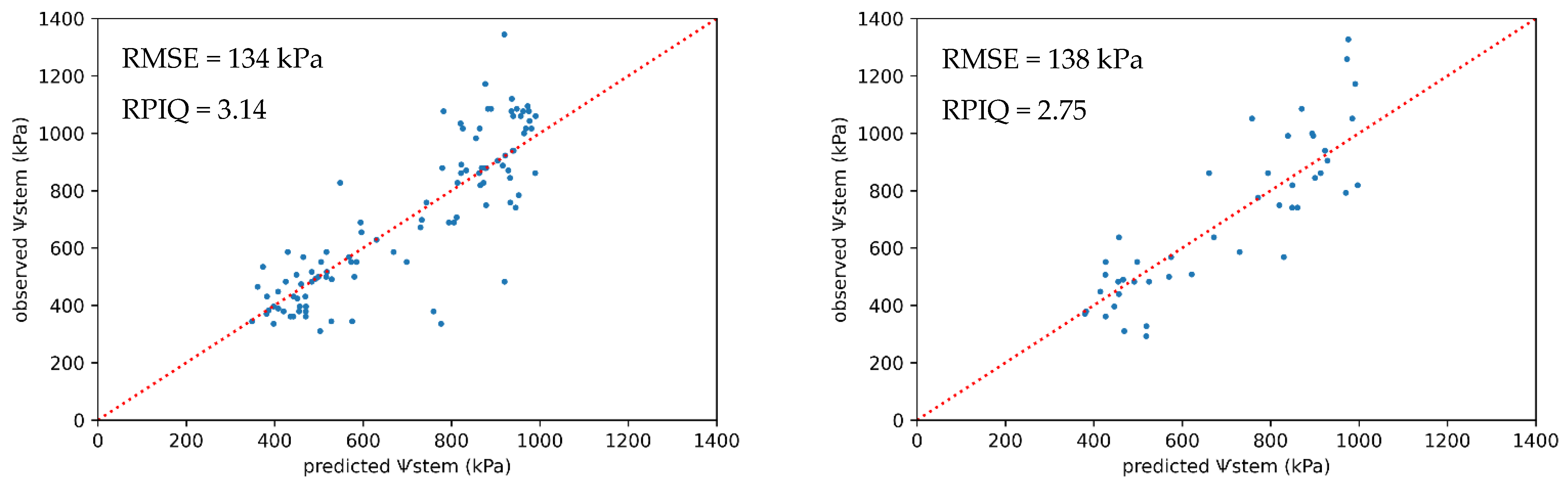
| ExG + full set of predictors | Support vector regression | 134 | 3.14 | 138 | 2.75 |
| ExG + soil/terrain + weather | Random forest regression | 139 | 3.02 | 142 | 2.66 |
| ExG + soil/terrain + temporal | Support vector regression | 135 | 3.10 | 141 | 2.69 |
| ExG + weather + temporal | Support vector regression | 138 | 3.03 | 143 | 2.65 |
| ExG + soil/terrain | Random forest regression | 196 | 2.14 | 214 | 1.77 |
| ExG + temporal | Random forest regression | 128 | 3.27 | 159 | 2.39 |
| ExG + weather | Random forest regression | 138 | 3.04 | 144 | 2.64 |
Publisher’s Note: MDPI stays neutral with regard to jurisdictional claims in published maps and institutional affiliations. |
© 2022 by the authors. Licensee MDPI, Basel, Switzerland. This article is an open access article distributed under the terms and conditions of the Creative Commons Attribution (CC BY) license (https://creativecommons.org/licenses/by/4.0/).
Share and Cite
Wei, H.-E.; Grafton, M.; Bretherton, M.; Irwin, M.; Sandoval, E. Evaluation of the Use of UAV-Derived Vegetation Indices and Environmental Variables for Grapevine Water Status Monitoring Based on Machine Learning Algorithms and SHAP Analysis. Remote Sens. 2022, 14, 5918. https://doi.org/10.3390/rs14235918
Wei H-E, Grafton M, Bretherton M, Irwin M, Sandoval E. Evaluation of the Use of UAV-Derived Vegetation Indices and Environmental Variables for Grapevine Water Status Monitoring Based on Machine Learning Algorithms and SHAP Analysis. Remote Sensing. 2022; 14(23):5918. https://doi.org/10.3390/rs14235918
Chicago/Turabian StyleWei, Hsiang-En, Miles Grafton, Mike Bretherton, Matthew Irwin, and Eduardo Sandoval. 2022. "Evaluation of the Use of UAV-Derived Vegetation Indices and Environmental Variables for Grapevine Water Status Monitoring Based on Machine Learning Algorithms and SHAP Analysis" Remote Sensing 14, no. 23: 5918. https://doi.org/10.3390/rs14235918
APA StyleWei, H.-E., Grafton, M., Bretherton, M., Irwin, M., & Sandoval, E. (2022). Evaluation of the Use of UAV-Derived Vegetation Indices and Environmental Variables for Grapevine Water Status Monitoring Based on Machine Learning Algorithms and SHAP Analysis. Remote Sensing, 14(23), 5918. https://doi.org/10.3390/rs14235918