A Method for the Automatic Extraction of Support Devices in an Overhead Catenary System Based on MLS Point Clouds

Abstract
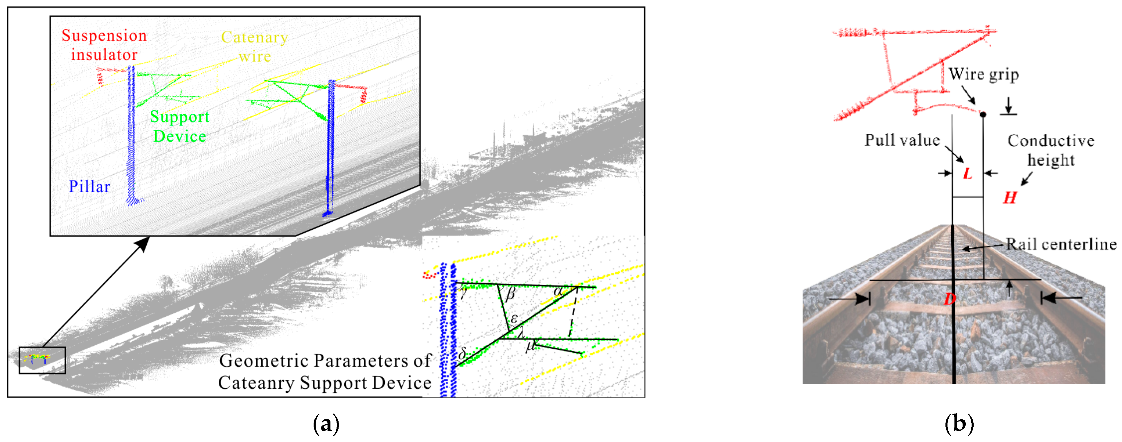
1. Introduction
- (1)
- A new method is proposed for locating support devices based on relatively stable spatial relationships between railway devices. Because each support device has a pillar center point, combining the two retrievals can reduce the occurrence of missing support devices and repeated extraction.
- (2)
- To achieve the high-precision extraction of the support device, other railway devices in the initial extraction results are filtered out by integrating two filters, the pillar and the voxel projection, which significantly improves the extraction accuracy of the support device. Among them, the voxel scale of the voxel projection filter is re-analyzed and designed based on the characteristics of the contact wires in the scene.
- (3)
- To assess the extraction effect and robustness of the proposed algorithm, six types of support devices and three types of support device distribution scenes are tested. Furthermore, two groups of railway unit scenes are tested to detect the performance of the algorithm in the actual application process.
2. Method
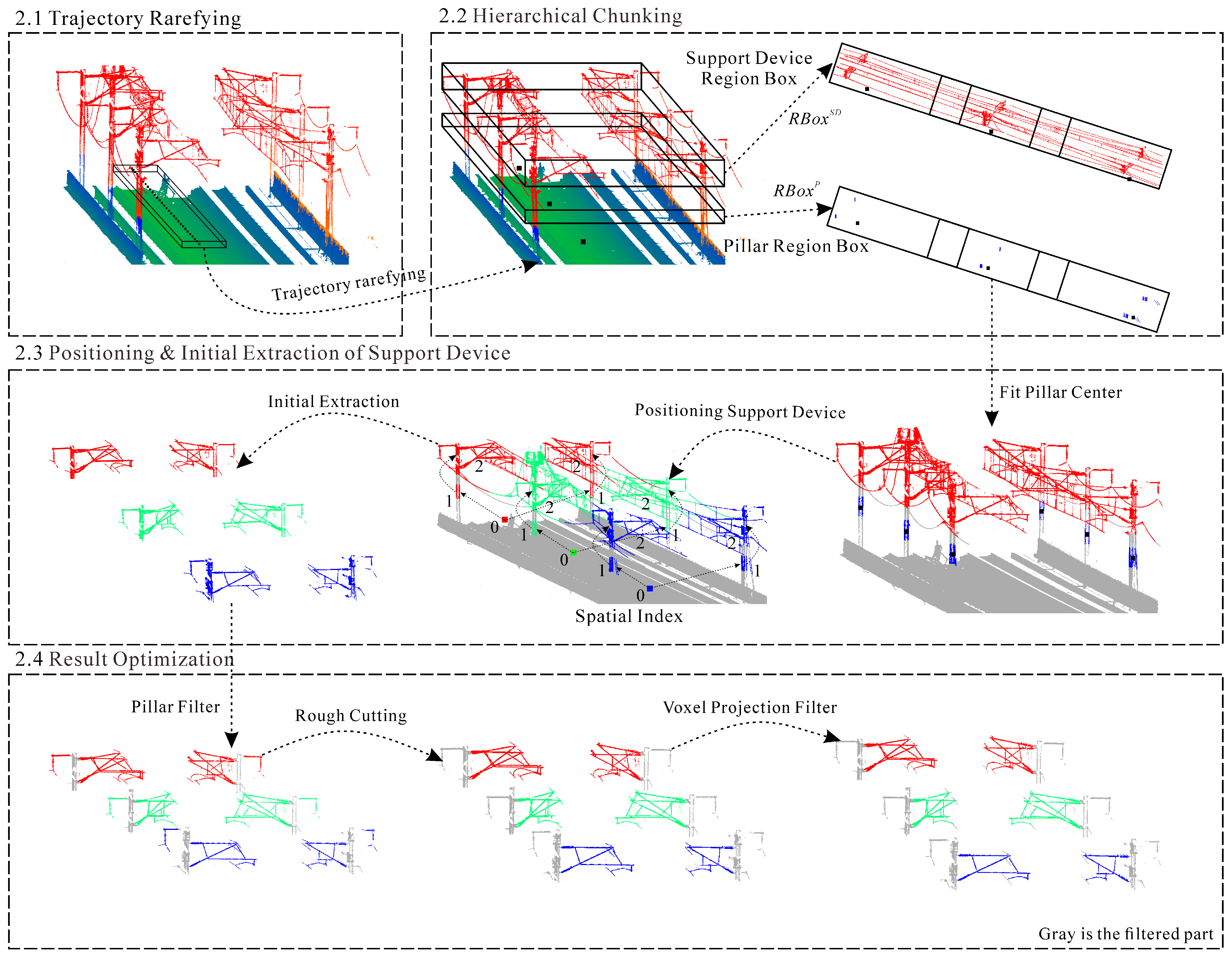
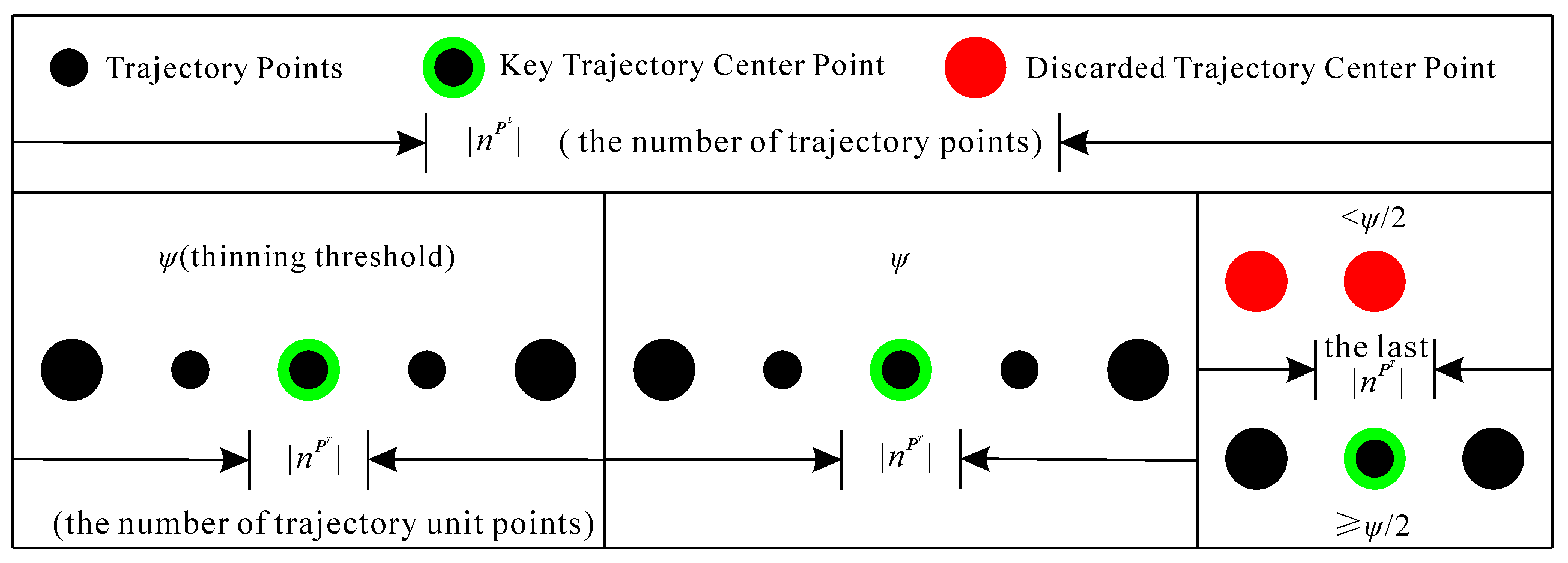
2.1. Trajectory Rarefying
2.2. Hierarchical Chunking
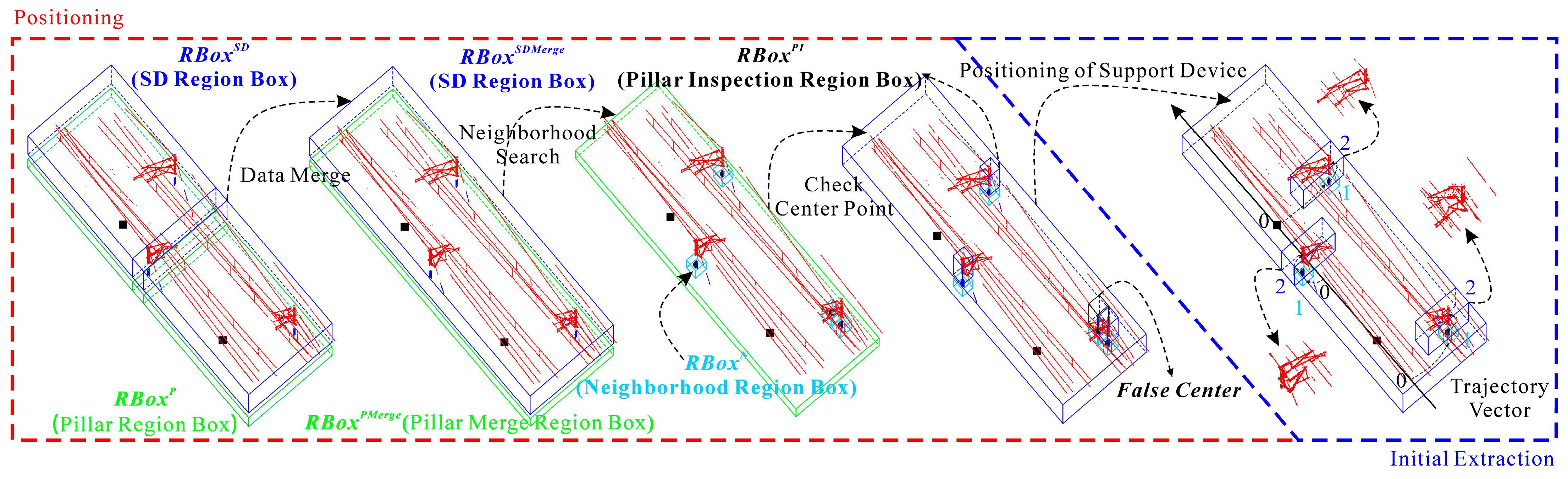
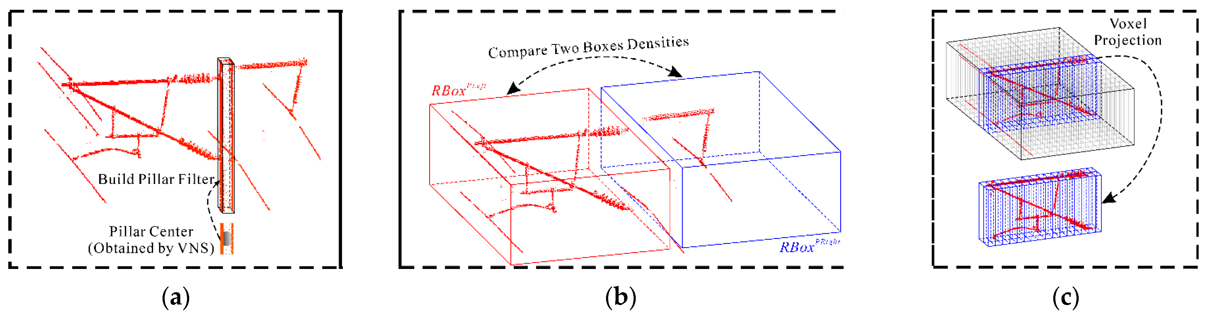
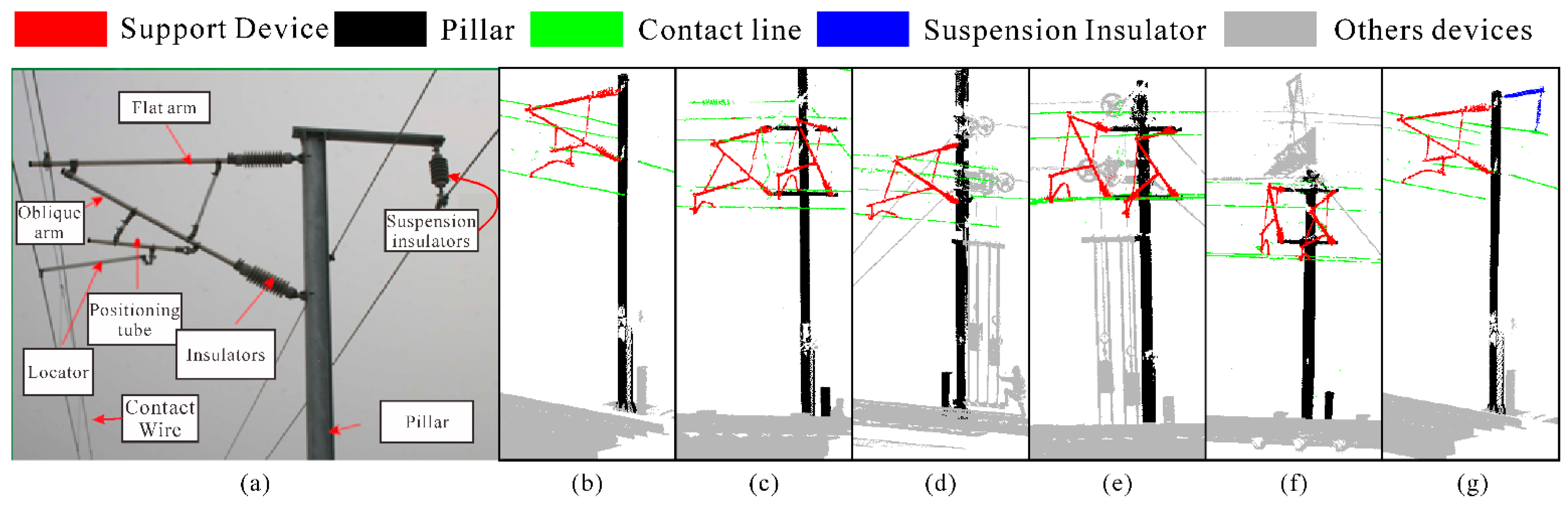
2.3. Positioning and Initial Extraction of the Support Device
| Algorithm 1. Algorithm for extracting pillar center points | |||||
| Input: | pillar region box: ; OCS-SD region box: ; neighborhood region box: ; pillar inspection region box: ; key trajectory center points set: , where is the total amount of . | ||||
| Output: | set of pillar center points: . | ||||
| 1: | fori = 1 to do | ||||
| 2: | initialize ; | ||||
| 3: | initialize ; | ||||
| 4: | for j = 0 to do | ||||
| 5: | if () then | ||||
| 6: | initialize k = 0; | ||||
| 7: | k++; | ||||
| 8: | Add to the collection; | ||||
| 9: | end if | ||||
| 10: | end for | ||||
| 11: | if () then is the pillar center point initial extraction threshold in | ||||
| 12: | Obtain the initial pillar center points | ||||
| 13: | end if | ||||
| 14: | end for | ||||
| 15: | fori = 0 to do | ||||
| 16: | for j = 0 to do | ||||
| 17: | initialize k = 0; | ||||
| 18: | if () | ||||
| 19: | k++; | ||||
| 20: | end if | ||||
| 21: | if () is the pillar center point check threshold in | ||||
| 22: | |||||
| 23: | end if | ||||
| 24: | end for | ||||
| 25: | end for | ||||
| 26: | return; | ||||
2.4. Result Optimization
3. Experiments
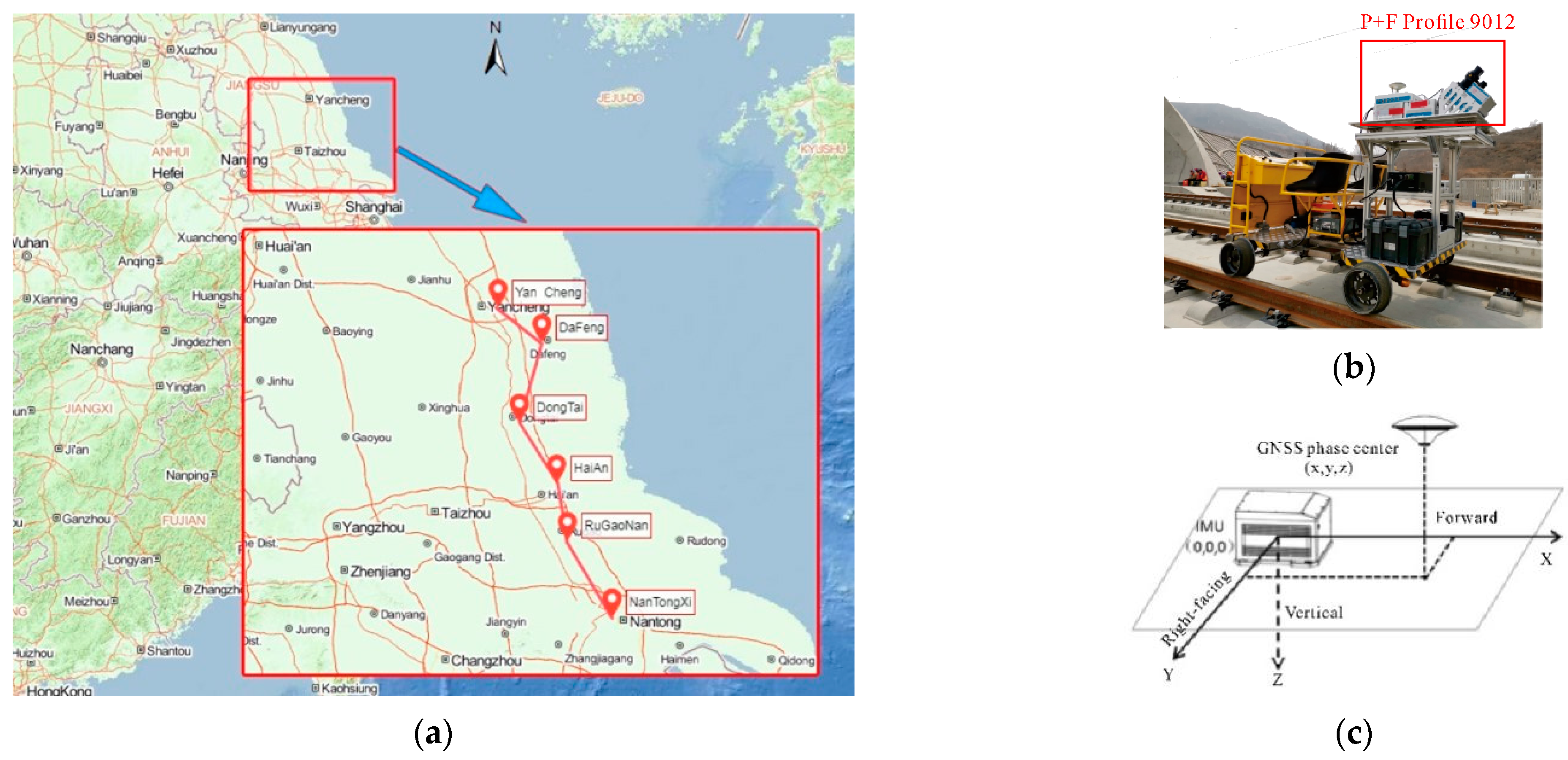
3.1. Study Area and Dataset
3.2. Implemental Details
3.3. Evaluation Indexes
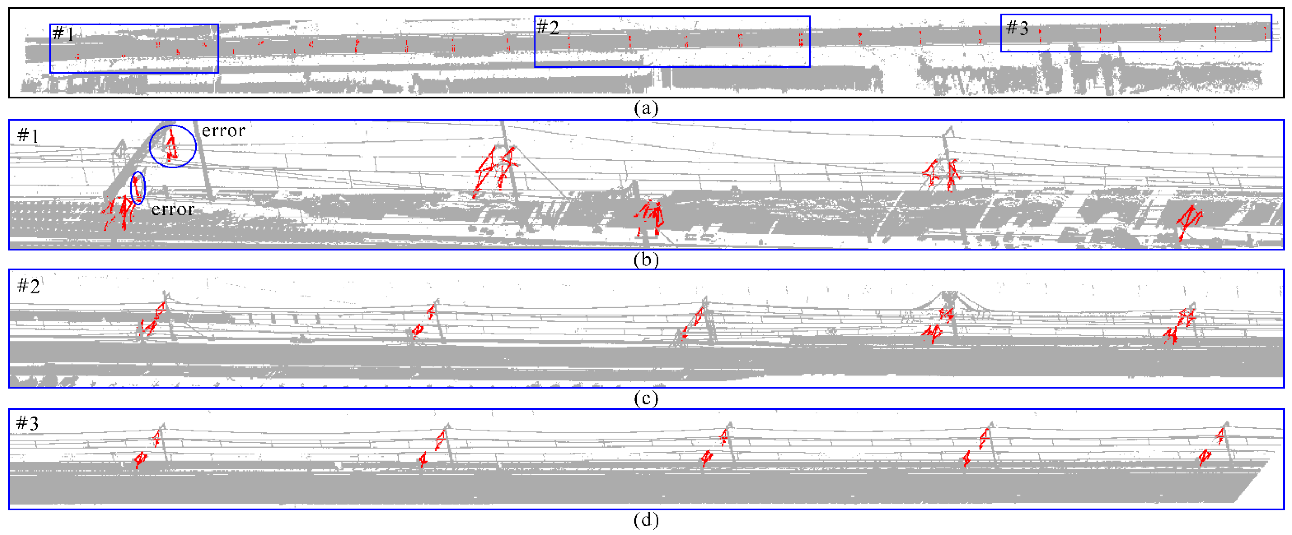
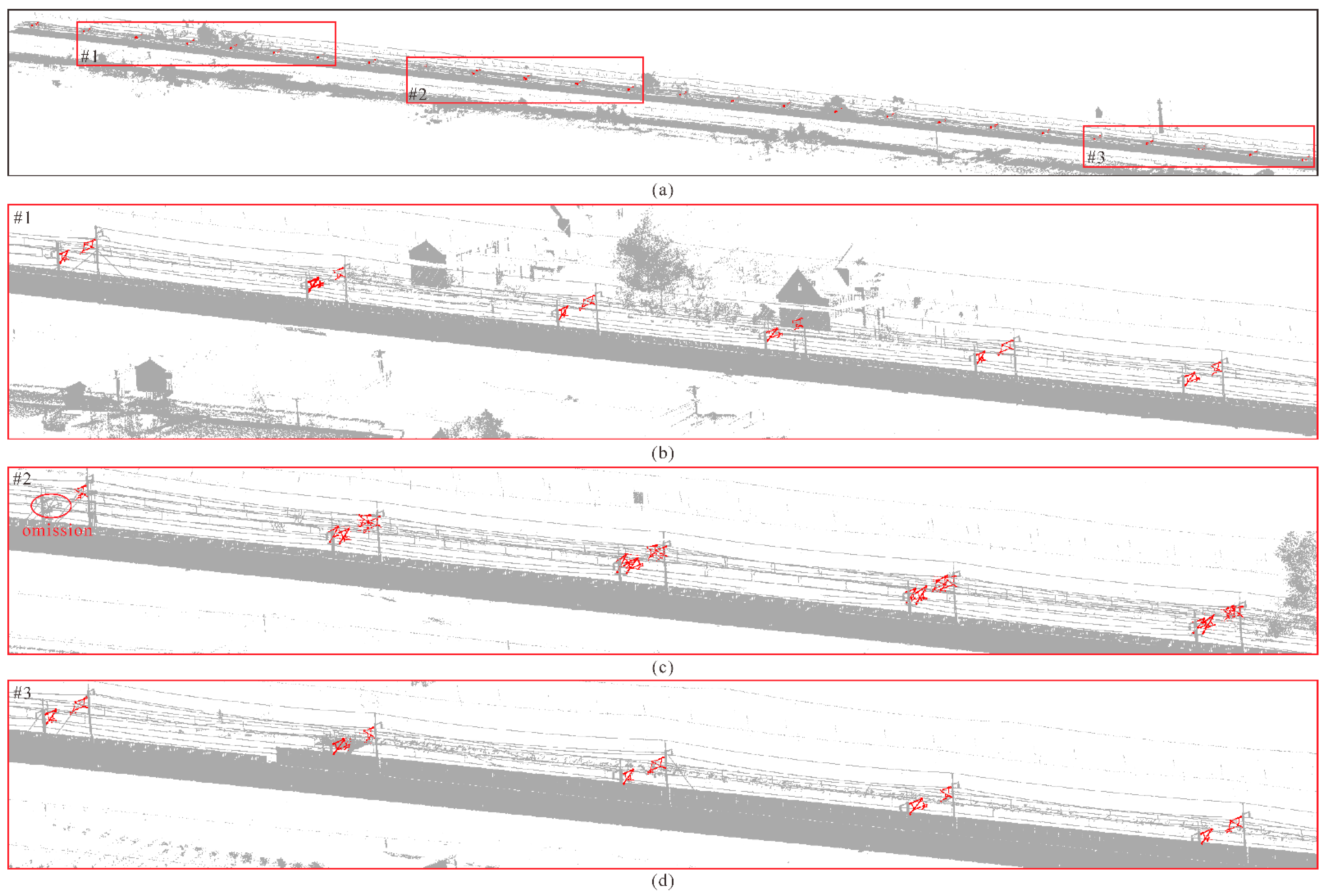
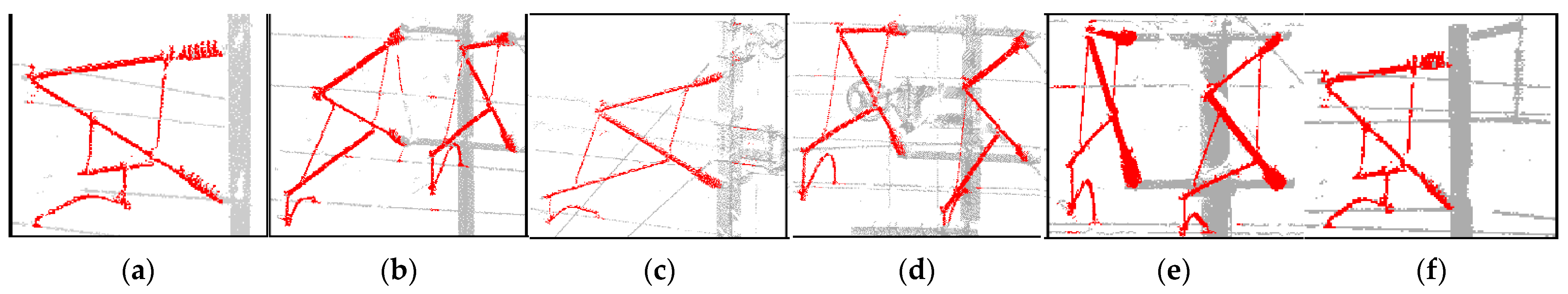
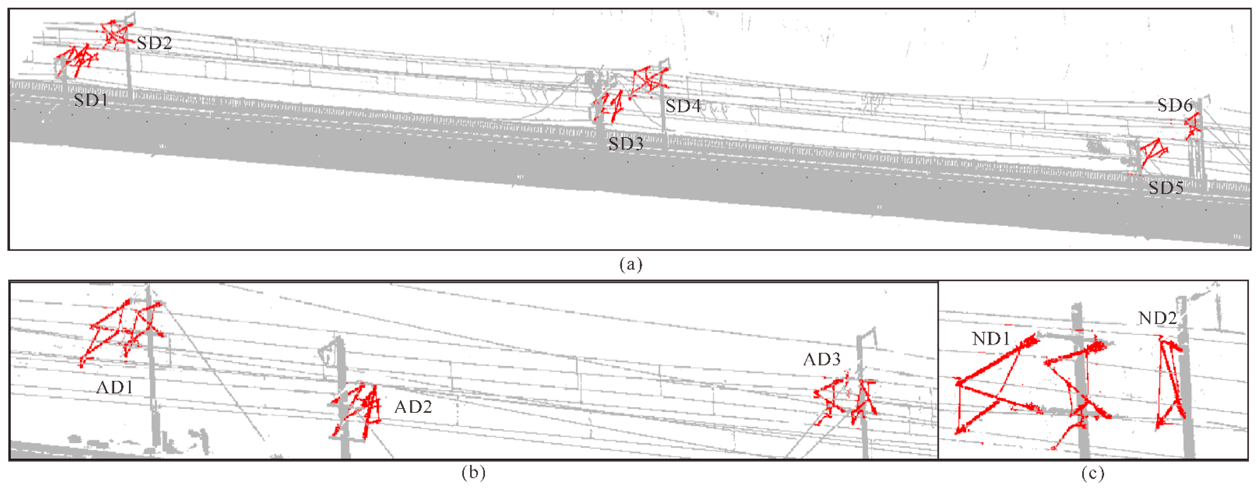
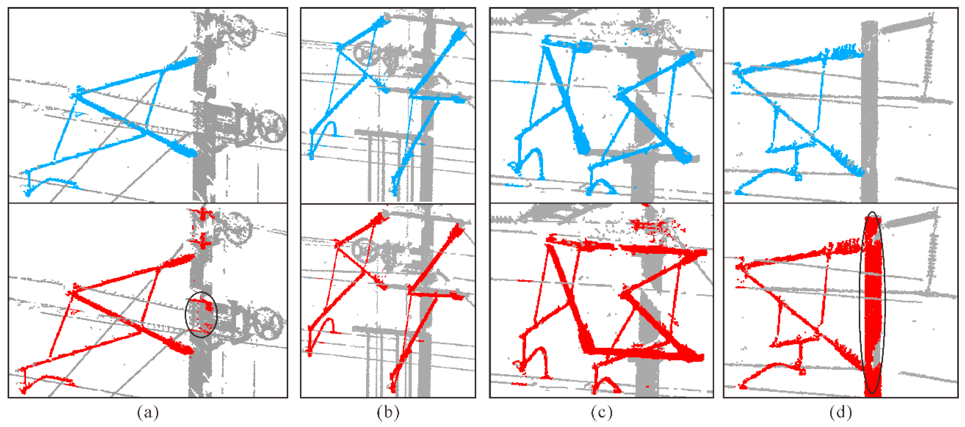
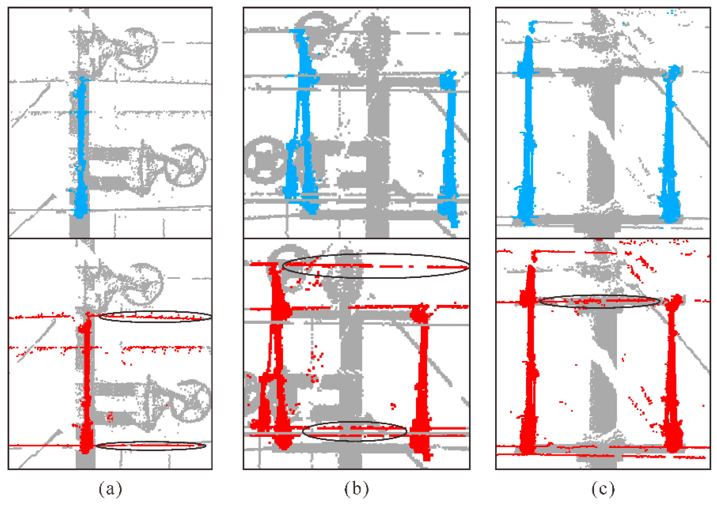
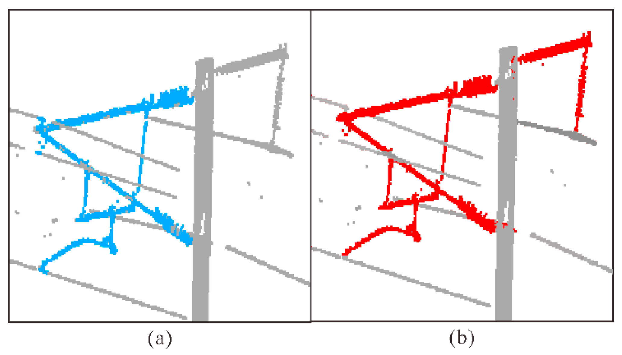
3.4. Experimental Results
3.5. Ablation Experiments
4. Discussion
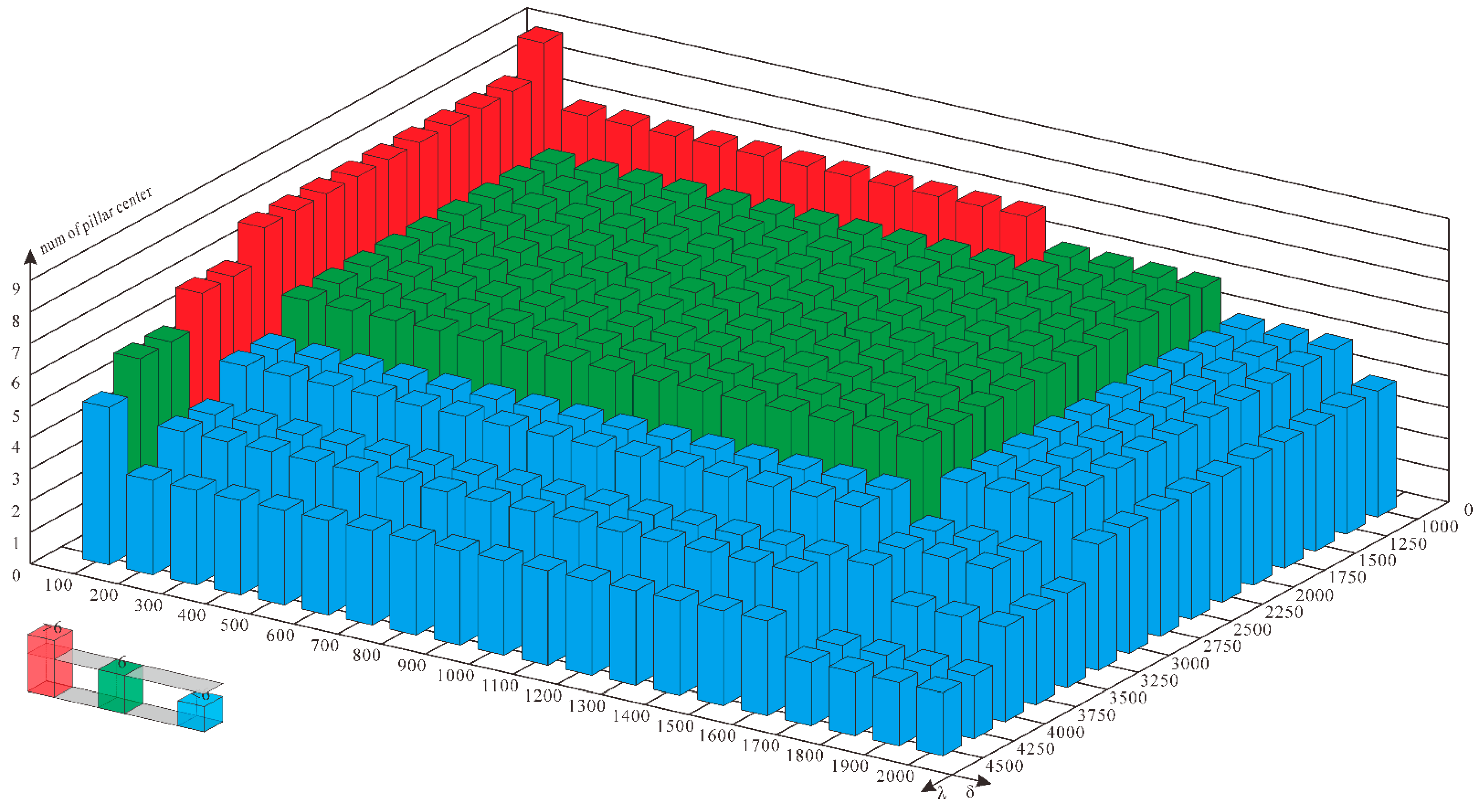
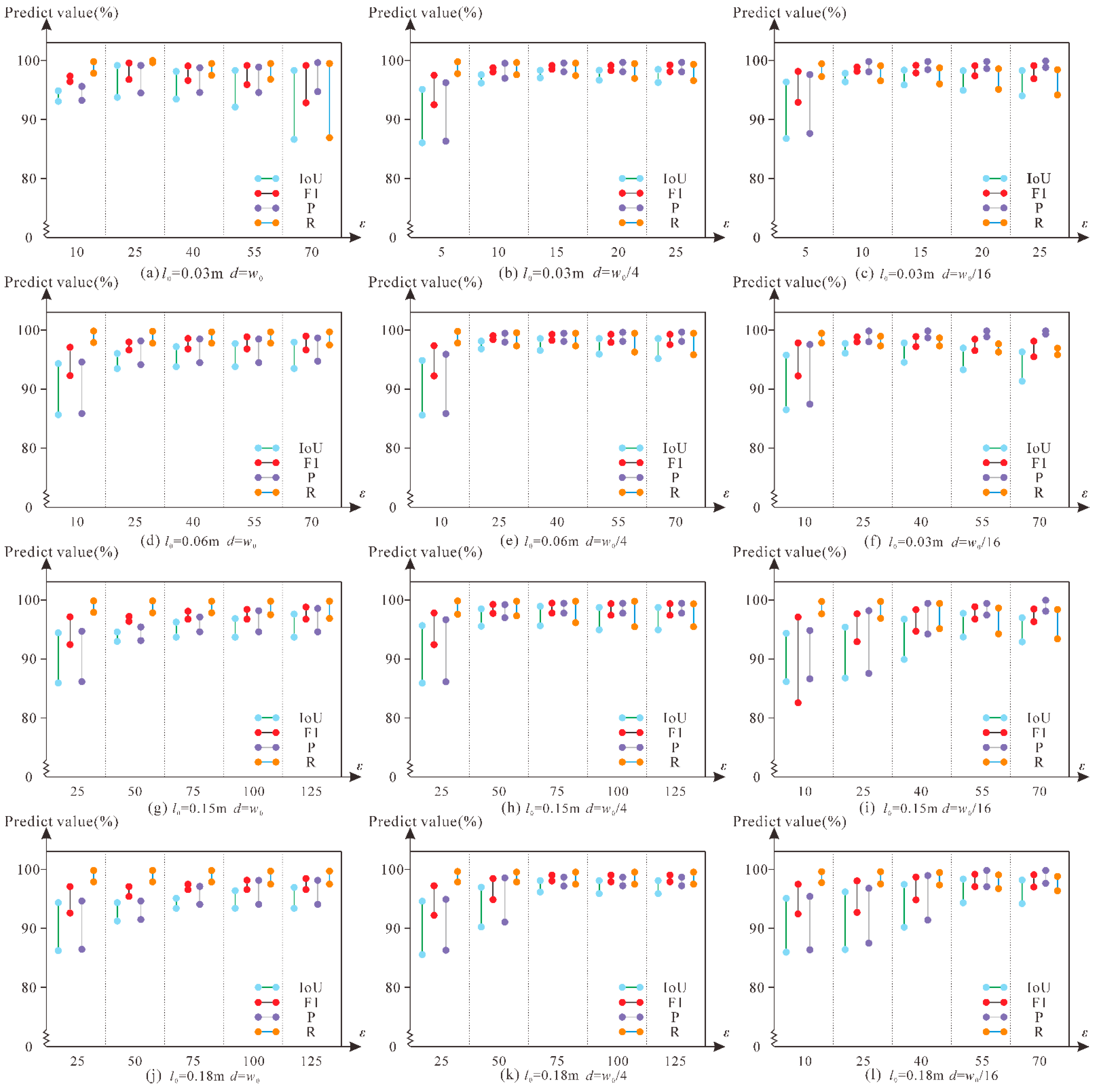
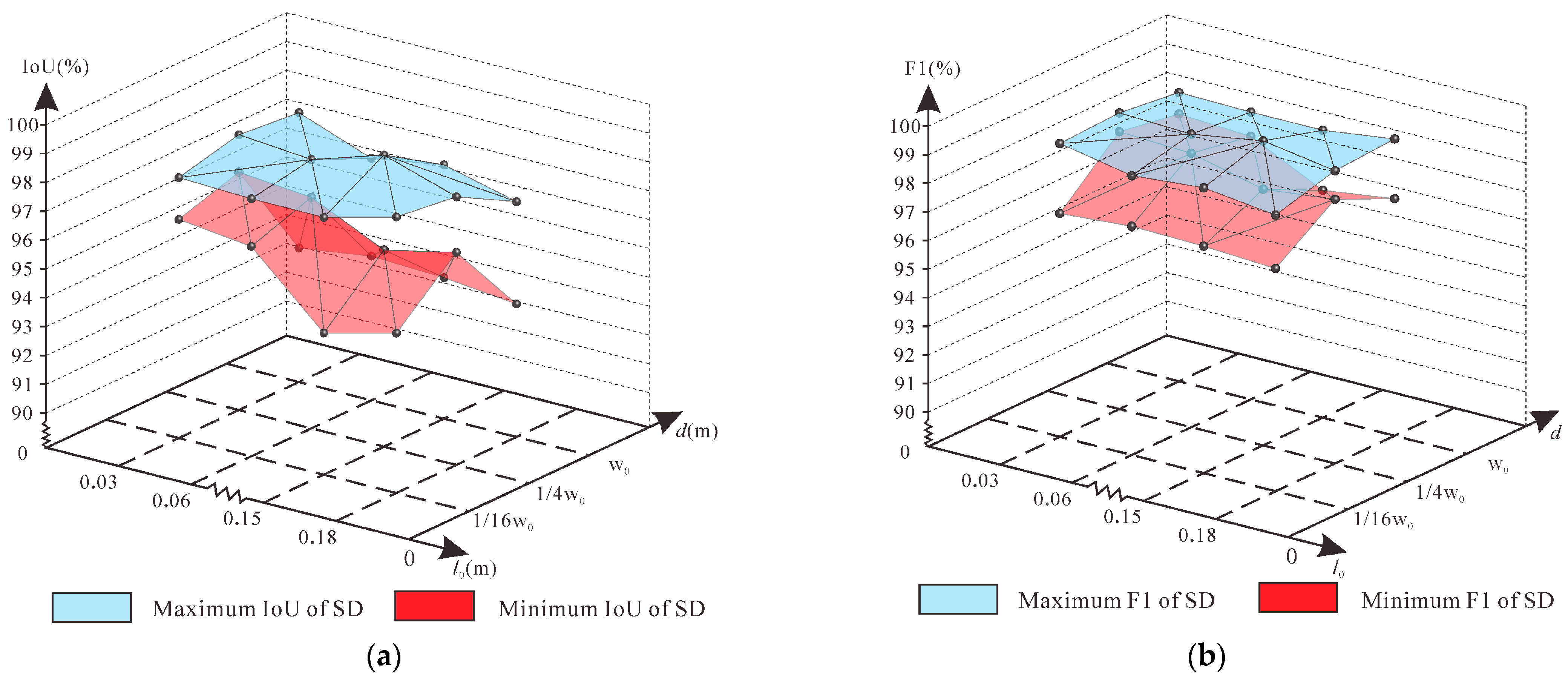
4.1. Analysis of Rarefying Threshold
4.2. Analysis of the Thresholds of the Pillar Center Points
4.3. Analysis of Voxel Size and Contact Line Threshold
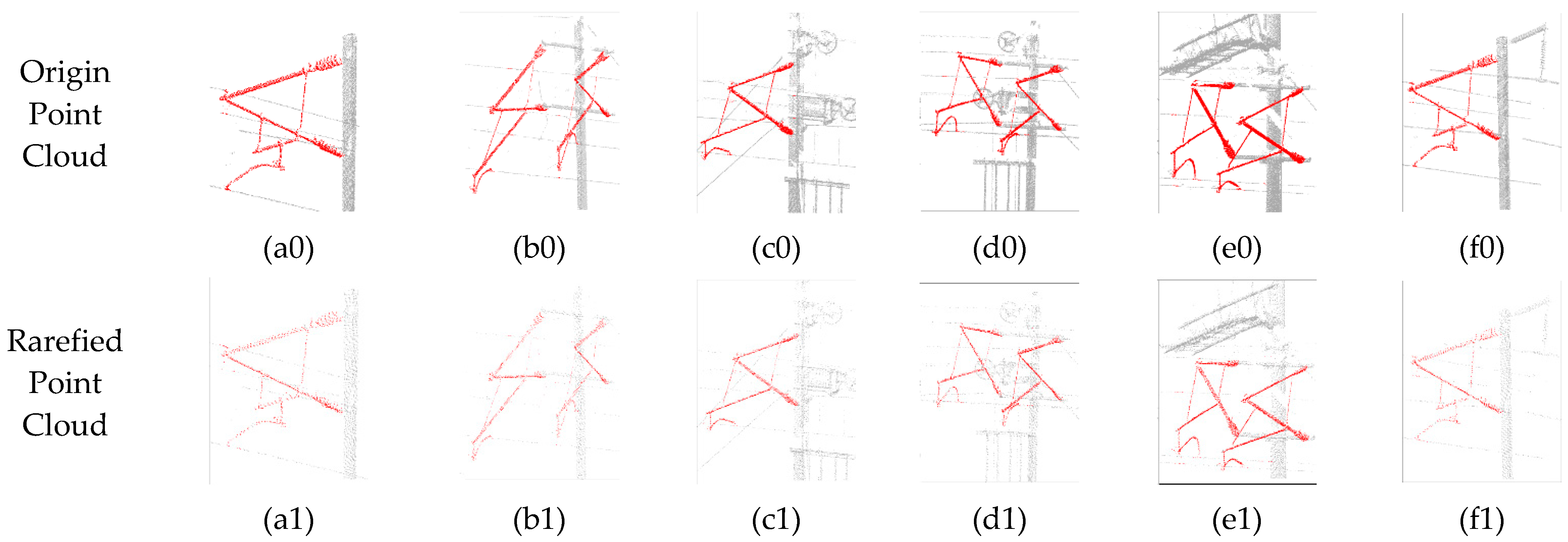
4.4. Discussion on Point Sparsity
5. Conclusions
Author Contributions
Funding
Conflicts of Interest
References
- Boccardo, P.; Arneodo, F.; Botta, D. Application of Geomatic techniques in Infomobility and Intelligent Transport Systems (ITS). Eur. J. Remote Sens. 2014, 47, 95–115. [Google Scholar] [CrossRef]
- Arco, E.; Ajmar, A.; Arneodo, F.; Boccardo, P. An operational framework to integrate traffic message channel (TMC) in emergency mapping services (EMS). Eur. J. Remote Sens. 2017, 50, 478–495. [Google Scholar] [CrossRef]
- Sánchez-Vaquerizo, J.A. Getting Real: The Challenge of Building and Validating a Large-Scale Digital Twin of Barcelona’s Traffic with Empirical Data. ISPRS Int. J. Geo-Inf. 2022, 11, 24. [Google Scholar] [CrossRef]
- Fang, L.N.; Chen, H.; Luo, H.; Guo, Y.Y.; Li, J. An intensity-enhanced method for handling mobile laser scanning point clouds. Int. J. Appl. Earth Obs. Geoinf. 2022, 107, 102684. [Google Scholar] [CrossRef]
- Qin, X.Q.; Li, Q.Q.; Ding, X.L.; Xie, L.F.; Wang, C.S.; Liao, M.S.; Zhang, L.; Zhang, B.; Xiong, S. A structure knowledge-synthetic aperture radar interferometry integration method for high-precision deformation monitoring and risk identification of sea-crossing bridges. Int. J. Appl. Earth Obs. Geoinf. 2021, 103, 102476. [Google Scholar] [CrossRef]
- Wang, J.; Zhao, H.R.; Wang, D.; Chen, Y.Y.; Zhang, Z.Q.; Liu, H. GPS trajectory-based segmentation and multi-filter-based extraction of expressway curbs and markings from mobile laser scanning data. Eur. J. Remote Sens. 2018, 51, 1022–1035. [Google Scholar]
- Liu, Z.G.; Song, Y.; Han, Y.; Wang, H.R.; Zhang, J.; Han, Z.W. Advances of research on high-speed railway catenary. J. Mod. Transp. 2017, 26, 1–23. [Google Scholar] [CrossRef]
- Midya, S.; Bormann, D.; Schutte, T.; Thottappillil, R. Pantograph Arcing in Electrified Railways-Mechanism and Influence of Various Parameters-Part I: With DC Traction Power Supply. IEEE Trans. Power Deliv. 2009, 24, 1931–1939. [Google Scholar] [CrossRef]
- Cheng, M.; Zhang, H.C.; Wang, C.; Li, J. Extraction and Classification of Road Markings Using Mobile Laser Scanning Point Clouds. IEEE J. Sel. Top. Appl. Earth Obs. Remote Sens. 2017, 10, 1182–1196. [Google Scholar] [CrossRef]
- Wen, C.L.; Sun, X.T.; Li, J.; Wang, C.; Guo, Y.; Habib, A. A deep learning framework for road marking extraction, classification and completion from mobile laser scanning point clouds. ISPRS J. Photogramm. Remote Sens. 2019, 147, 178–192. [Google Scholar] [CrossRef]
- Meng, X.L.; Currit, N.; Zhao, K.G. Ground Filtering Algorithms for Airborne LiDAR Data: A Review of Critical Issues. Remote Sens. 2010, 2, 833–860. [Google Scholar] [CrossRef]
- Chen, D.; Zhang, L.Q.; Mathiopoulos, P.T.; Huang, X.F. A Methodology for Automated Segmentation and Reconstruction of Urban 3-D Buildings from ALS Point Clouds. IEEE J. Sel. Top. Appl. Earth Obs. Remote Sens. 2014, 7, 4199–4217. [Google Scholar] [CrossRef]
- Cui, H.; Li, J.; Hu, Q.W.; Mao, Q.Z. Real-Time Inspection System for Ballast Railway Fasteners Based on Point Cloud Deep Learning. IEEE Access 2020, 8, 61604–61614. [Google Scholar] [CrossRef]
- Nurunnabi, A.A.M.; Teferle, N.; Li, J.; Lindenbergh, R.C.; Hunegnaw, A. An efficient deep learning approach for ground point filtering in aerial laser scanning point clouds. Int. Arch. Photogramm. Remote Sens. Spat. Inf. Sci. ISPRS Arch. 2021, 43, 31–38. [Google Scholar] [CrossRef]
- Jenke, P.; Wand, M.; Bokeloh, M.; Schilling, A.; Straßer, W. Bayesian Point Cloud Reconstruction. Comput. Graph. Forum 2006, 25, 379–388. [Google Scholar] [CrossRef]
- Han, X.F.; Jin, J.S.; Wang, M.J.; Jiang, W.; Gao, L.; Xiao, L.P. A review of algorithms for filtering the 3D point cloud. Signal Process. Image Commun. 2017, 57, 103–112. [Google Scholar] [CrossRef]
- Schall, O.; Belyaev, A.; Seidel, H.P. Adaptive feature-preserving non-local denoising of static and time-varying range data. Comput.-Aided Des. 2008, 40, 701–707. [Google Scholar] [CrossRef]
- Liao, B.; Xiao, C.X.; Jin, L.Q.; Fu, H.B. Efficient feature-preserving local projection operator for geometry reconstruction. Comput.-Aided Des. 2013, 45, 861–874. [Google Scholar] [CrossRef]
- Xiao, C.X.; Miao, Y.W.; Liu, S.; Peng, Q.S. A dynamic balanced flow for filtering point-sampled geometry. Vis. Comput. 2006, 22, 210–219. [Google Scholar] [CrossRef]
- Jaafary, A.H.; Salehi, M.R. Analysis of an All-Optical Microwave Mixing and Bandpass Filtering with Negative Coefficients. In Proceedings of the 2007 IEEE International Conference on Signal Processing and Communications, Dubai, United Arab Emirates, 24–27 November 2007; pp. 1123–1126. [Google Scholar]
- Zhang, L.Y.; Chang, J.H.; Li, H.X.; Liu, Z.X.; Zhang, S.Y.; Mao, R. Noise Reduction of LiDAR Signal via Local Mean Decomposition Combined with Improved Thresholding Method. IEEE Access 2020, 8, 113943–113952. [Google Scholar] [CrossRef]
- Barca, E.; Castrignanò, A.; Ruggieri, S.; Rinaldi, M. A new supervised classifier exploiting spectral-spatial information in the Bayesian framework. Int. J. Appl. Earth Obs. Geoinf. 2020, 86, 101990. [Google Scholar] [CrossRef]
- Zhao, G.Q.; Xiao, X.H.; Yuan, J.S. Fusion of Velodyne and camera data for scene parsing. In Proceedings of the 2012 15th International Conference on Information Fusion, Singapore, 9–12 July 2012; pp. 1172–1179. [Google Scholar]
- Li, R.; Qi, R.; Liu, L.P. Point Cloud De-Noising Based on Three-Dimensional Projection. In Proceedings of the 2015 International Conference on Computational Intelligence and Communication Networks (CICN), Jabalpur, India, 12–14 December 2015; pp. 942–946. [Google Scholar]
- Jiang, X.Y.; Meier, U.; Bunke, H. Fast Range Image Segmentation Using High-Level Segmentation Primitives. In Proceedings of the Third IEEE Workshop on Applications of Computer Vision WACV, Sarasoto, FL, USA, 2–4 December 1996; pp. 83–88. [Google Scholar]
- Zhang, R.; Li, G.Y.; Wunderlich, T.; Wang, L. A survey on deep learning-based precise boundary recovery of semantic segmentation for images and point clouds. Int. J. Appl. Earth Obs. Geoinf. 2021, 102, 102411. [Google Scholar] [CrossRef]
- Xia, Y.Q.; Xie, X.W.; Wu, X.W.; Zhi, J.; Qiao, S.H. An Approach of Automatically Selecting Seed Point Based on Region Growing for Liver Segmentation. In Proceedings of the 2019 8th International Symposium on Next Generation Electronics (ISNE), Zhengzhou, China, 9–10 October 2019; pp. 1–4. [Google Scholar]
- Vo, A.; Truong-Hong, L.; Laefer, D.F.; Bertolotto, M. Octree-based region growing for point cloud segmentation. ISPRS J. Photogramm. Remote Sens. 2015, 104, 88–100. [Google Scholar] [CrossRef]
- Zhao, B.F.; Hua, X.H.; Yu, K.G.; Xuan, W.; Chen, X.J.; Tao, W.J. Indoor Point Cloud Segmentation Using Iterative Gaussian Mapping and Improved Model Fitting. IEEE Trans. Geosci. Remote Sens. 2020, 58, 7890–7907. [Google Scholar] [CrossRef]
- Ma, X.F.; Luo, W.; Chen, M.Q.; Li, J.H.; Yan, X.; Zhang, X.; Wei, W. A Fast Point Cloud Segmentation Algorithm Based on Region Growth. In Proceedings of the 2019 18th International Conference on Optical Communications and Networks (ICOCN), Huangshan, China, 5–8 August 2019; pp. 1–2. [Google Scholar]
- Sun, S.P.; Li, C.Y.; Chee, P.W.; Paterson, A.H.; Jiang, Y.; Xu, R.; Robertson, J.S.; Adhikari, J.; Shehzad, T. Three-dimensional photogrammetric mapping of cotton bolls in situ based on point cloud segmentation and clustering. ISPRS J. Photogramm. Remote Sens. 2020, 160, 195–207. [Google Scholar] [CrossRef]
- Xu, L.; Oja, E.; Kultanen, P. A new curve detection method: Randomized Hough transform (RHT). Pattern Recognit. Lett. 1990, 11, 331–338. [Google Scholar] [CrossRef]
- Filin, S. Surface classification from airborne laser scanning data. Comput. Geosci. 2004, 30, 1033–1041. [Google Scholar] [CrossRef]
- Biosca, J.M.; Lerma, J.L. Unsupervised robust planar segmentation of terrestrial laser scanner point clouds based on fuzzy clustering methods. ISPRS J. Photogramm. Remote Sens. 2007, 63, 84–98. [Google Scholar] [CrossRef]


| Parameter | Description | Value |
|---|---|---|
| support device region box (affine transformation is required) | length: 30 m, width: 22 m, height: 1.0 m | |
| pillar region box (affine transformation is required) | length: 30 m, width: 22 m, height: 3.5 m | |
| neighborhood region box | length: 0.8 m, width: 0.8 m, height: 2.0 m | |
| pillar inspection region box | length: 0.4 m, width: 0.4 m, height: 3.5 m | |
| pillar filter region box | length: 0.4 m, width: 2.6 m, height: 3.5 m | |
| the left region box adjacent to | length: 6.2 m, width: 3.0 m, height: 3.5 m | |
| the right region box adjacent to | length: 6.2 m, width: 3.0 m, height: 3.5 m | |
| the initial extraction region box of the support device | length: 12.8 m, width: 3.0 m, height: 3.5 m | |
| the rarefying threshold of trajectory data | 10 | |
| pillar center point initial extraction threshold in | 1200 | |
| pillar center point check threshold in | 2500 | |
| voxel width | 1/16 | |
| contact line rejection threshold in voxel | 25 | |
| voxel length | 0.06 m |
| Types | SSD | DSD | SRSD | DRSD | SFSD | LSD | Average | |
|---|---|---|---|---|---|---|---|---|
| Predict (%) | ||||||||
| P (%) | 99.59 | 98.02 | 99.74 | 99.74 | 98.76 | 99.83 | 99.28 | |
| R (%) | 97.53 | 97.97 | 97.70 | 96.52 | 98.94 | 97.38 | 97.67 | |
| F1 (%) | 97.14 | 98 | 98.71 | 98.1 | 98.85 | 98.59 | 98.23 | |
| IoU (%) | 98.55 | 96.08 | 97.46 | 96.28 | 97.73 | 97.23 | 97.22 |
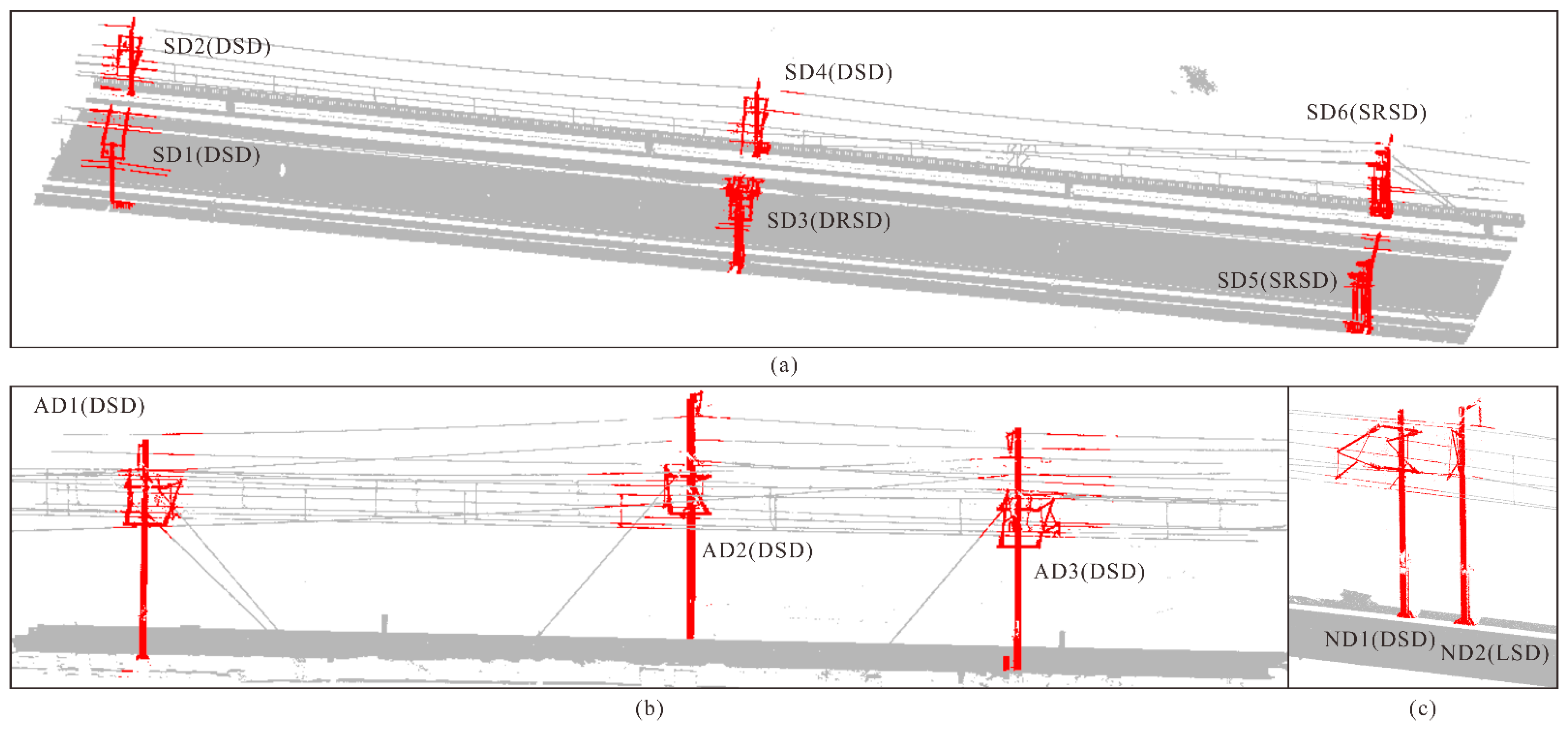
| Scene | SD | AD | ND | ||||||||||||
|---|---|---|---|---|---|---|---|---|---|---|---|---|---|---|---|
| Predict | SD1 | SD2 | SD3 | SD4 | SD5 | SD6 | Average | AD1 | AD2 | AD3 | Average | ND1 | ND2 | Average | |
| P (%) | 99.08 | 99.85 | 99.72 | 98.09 | 95.07 | 99.12 | 98.48 | 98.40 | 99.43 | 98.85 | 98.89 | 98.05 | 97.77 | 97.91 | |
| R (%) | 99.13 | 98.18 | 96.75 | 99.78 | 95.64 | 93.84 | 97.21 | 97.87 | 93.35 | 95.31 | 95.51 | 98.56 | 90.12 | 94.34 | |
| F1 (%) | 99.11 | 99.01 | 98.21 | 98.92 | 95.64 | 96.41 | 97.88 | 98.13 | 96.29 | 97.05 | 97.15 | 98.3 | 93.79 | 96.05 | |
| IoU (%) | 98.24 | 98.04 | 96.49 | 97.88 | 91.64 | 93.07 | 95.89 | 96.34 | 92.85 | 94.28 | 94.49 | 96.67 | 88.31 | 92.49 | |
| Parameter | Experimental Results | ||||||||||
|---|---|---|---|---|---|---|---|---|---|---|---|
| n | 5 | 6 | 7 | 8 | 9 | 10 | 11 | 12 | 13 | 14 | 15 |
| dis (m) | 20 | 24 | 28 | 32 | 36 | 40 | 44 | 48 | 52 | 56 | 60 |
| RKTO | 1 | 5/6 | 5/6 | 2/3 | 2/3 | 1/2 | 1/2 | 1/2 | 1/3 | 1/3 | 1/3 |
| Running time (s) | 1030 | 1010 | 990 | 990 | 980 | 980 | 980 | 970 | 960 | 960 | 940 |
| Type | SSD | DSD | SRSD | DRSD | SFSD | LSD | Average | |
|---|---|---|---|---|---|---|---|---|
| Predict | ||||||||
| Origin points number | 105,112 | 270,310 | 454,728 | 835,883 | 995,035 | 106,517 | 461,264 | |
| Filtered points number | 21,023 | 54,062 | 90,946 | 167,177 | 199,007 | 21,304 | 92,253 | |
| Origin P (%) | 99.59 | 98.02 | 99.74 | 99.74 | 98.76 | 99.83 | 99.28 | |
| P (%) | 97.93 | 96.48 | 99.51 | 99.40 | 99.16 | 97.01 | 98.25 | |
| Origin R (%) | 97.53 | 97.97 | 97.70 | 96.52 | 98.94 | 97.38 | 97.67 | |
| R (%) | 95.43 | 98.16 | 94.61 | 96.63 | 97.98 | 94.69 | 96.25 | |
| Origin F1 (%) | 97.14 | 98.00 | 98.71 | 98.1 | 98.85 | 98.59 | 98.23 | |
| F1 (%) | 96.66 | 97.31 | 97.01 | 97.99 | 98.57 | 96.22 | 97.29 | |
| Origin IoU (%) | 98.55 | 96.08 | 97.46 | 96.28 | 97.73 | 97.23 | 97.22 | |
| IoU (%) | 93.55 | 94.77 | 94.18 | 96.07 | 97.18 | 92.72 | 94.75 | |
Publisher’s Note: MDPI stays neutral with regard to jurisdictional claims in published maps and institutional affiliations. |
© 2022 by the authors. Licensee MDPI, Basel, Switzerland. This article is an open access article distributed under the terms and conditions of the Creative Commons Attribution (CC BY) license (https://creativecommons.org/licenses/by/4.0/).
Share and Cite
Zhang, S.; Meng, Q.; Hu, Y.; Fu, Z.; Chen, L. A Method for the Automatic Extraction of Support Devices in an Overhead Catenary System Based on MLS Point Clouds. Remote Sens. 2022, 14, 5915. https://doi.org/10.3390/rs14235915
Zhang S, Meng Q, Hu Y, Fu Z, Chen L. A Method for the Automatic Extraction of Support Devices in an Overhead Catenary System Based on MLS Point Clouds. Remote Sensing. 2022; 14(23):5915. https://doi.org/10.3390/rs14235915
Chicago/Turabian StyleZhang, Shengyuan, Qingxiang Meng, Yulong Hu, Zhongliang Fu, and Lijin Chen. 2022. "A Method for the Automatic Extraction of Support Devices in an Overhead Catenary System Based on MLS Point Clouds" Remote Sensing 14, no. 23: 5915. https://doi.org/10.3390/rs14235915
APA StyleZhang, S., Meng, Q., Hu, Y., Fu, Z., & Chen, L. (2022). A Method for the Automatic Extraction of Support Devices in an Overhead Catenary System Based on MLS Point Clouds. Remote Sensing, 14(23), 5915. https://doi.org/10.3390/rs14235915