Patch-Based Discriminative Learning for Remote Sensing Scene Classification

Abstract

The research focus in remote sensing scene image classification has been recently shifting towards deep learning (DL) techniques. However, even the state-of-the-art deep-learning-based models have shown limited performance due to the inter-class similarity and the intra-class diversity among scene categories. To alleviate this issue, we propose to explore the spatial dependencies between different image regions and introduce patch-based discriminative learning (PBDL) for remote sensing scene classification. In particular, the proposed method employs multi-level feature learning based on small, medium, and large neighborhood regions to enhance the discriminative power of image representation. To achieve this, image patches are selected through a fixed-size sliding window, and sampling redundancy, a novel concept, is developed to minimize the occurrence of redundant features while sustaining the relevant features for the model. Apart from multi-level learning, we explicitly impose image pyramids to magnify the visual information of the scene images and optimize their positions and scale parameters locally. Motivated by this, a local descriptor is exploited to extract multi-level and multi-scale features that we represent in terms of a codeword histogram by performing k-means clustering. Finally, a simple fusion strategy is proposed to balance the contribution of individual features where the fused features are incorporated into a bidirectional long short-term memory (BiLSTM) network. Experimental results on the NWPU-RESISC45, AID, UC-Merced, and WHU-RS datasets demonstrate that the proposed approach yields significantly higher classification performance in comparison with existing state-of-the-art deep-learning-based methods.

1. Introduction

Remote sensing has received unprecedented attention due to its role in mapping land cover [1], geographic image retrieval [2], natural hazards’ detection [3], and monitoring changes in land cover [4]. The currently available remote sensing satellites and instruments (e.g., IKONOS, unmanned aerial vehicles (UAVs), synthetic aperture radar) for observing the Earth not only provide high-resolution scene images but also give us an opportunity to study the spatial information with a fine-grained detail [5].

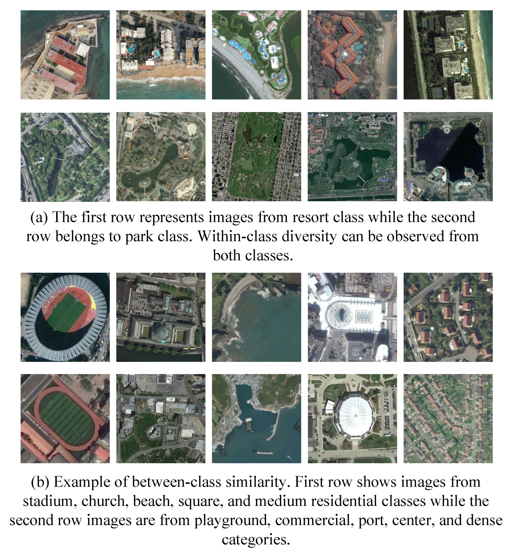
However, within-class diversity and between-class similarity among scene categories are the main challenges that make it extremely difficult to distinguish the scene classes. For instance, as shown in Figure 1a, a large intra-class or within-class diversity can be observed such as the resort scenes appearing in different building styles but all of them belong to the same class. Similarly, the park scenes show large differences within the same semantic class. In addition, satellite imagery data can be influenced by differences in color or radiation intensity due to factors such as weather, cloud coverage and mist, which, in turn, may cause within-class diversity [6,7]. In terms of inter-class or between-class similarity, the challenge is caused by the appearance of the same ground objects within the different scene classes as illustrated in Figure 1b. For instance, we can see that stadium and playground are different classes but represent a highly semantic overlapping between scene categories. This motivates us to focus on multi-level spatial features with small within-class scatter but large between-class separation. Here, the “scenes” belong to a different type of subareas extracted from large satellite images. These subareas could be different types of land covers or objects and possess a specific semantic meaning, such as commercial area, dense residential, sparse residential, and parking lot in a typical urban area of satellite image [6]. With the development of modern technologies, scene classification has been an active research field, and correctly labeling it to a predefined class is still a challenging task.

In the early days, most of the approaches focused on hand-crafted features, which can be computed based on shape, color, or textual characteristics where commonly used descriptors are local binary patterns (LBPs) [8], scale invariant feature transform [9], color histogram [10], or histogram oriented gradients (HOG) [11]. A major shortcoming of these low-level descriptors is their inability to fulfill scene understanding due to the high diversity and non-homogeneous spatial distributions of the scene classes. In comparison to handcrafted features, the bag-of-words (BoW) model is one of the famous mid-level (global) representations, which became extremely popular in image analysis and classification [12], while providing an efficient solution for aerial or satellite image scene classification [13]. It was first proposed for text analysis and then extended to images by a spatial pyramid method (SPM) because the vanilla BoW model does not consider spatial and structural information. Specifically, the SPM method divides the images into several parts and computes BoW histograms from each part based on the structure of local features. The histograms are then concatenated from all image parts to make up the final representation [14]. Although these mid-level features are highly efficient, they may not be able to characterize detailed structures and distinct patterns. For instance, some scene classes are represented mainly by individual objects, e.g., runway and airport in remote sensing datasets. As a result, the performance of BoW model remains limited when dealing with complex and challenging scene images.

Recently, deep-learning-based methods have been successfully utilized in scene classification and proven to be promising in extracting high-level features. For instance, Shi et al. [15] proposed a multi-level feature fusion method based on a lightweight convolution neural network to improve the classification performance of scene images. Yuan et al. [16] proposed a multi-subset feature fusion method to integrate the global and local information of the deep features. A dual-channel spectral feature extraction network is introduced in [17]. Their model employs a 3D convolution kernel to directly extract multi-scale spatial features. Then an adaptive fusion of spectral and spatial features is performed to improve the performance. These methods testify of the importance of deep-learning-based feature fusion. However, patch-based global feature learning has been never deeply investigated in the BoW framework. Moreover, the authors in [18] argued that convolutional layers record a precise position of features in the input and generate a fixed-dimensional representation in the CNN framework. Since the pooling process decreases the size of the feature matrix after the convolution layer, the performance of CNN remains limited in the case where key features are minute and irregular [19]. One of the reasons is that natural images can be mainly captured by cameras with manual or auto-focus options, which make them center-biased [20]. However, in the case of remote sensing scene classification, images are usually captured overhead. Therefore, using a CNN as a “black box” to classify remote sensing images may be not good enough for complex scenes. Even though several works [21,22] attempted to focus on critical local image patches, the role of the spatial dependency among objects in remote sensing scene classification task remains an unsolved problem [23].

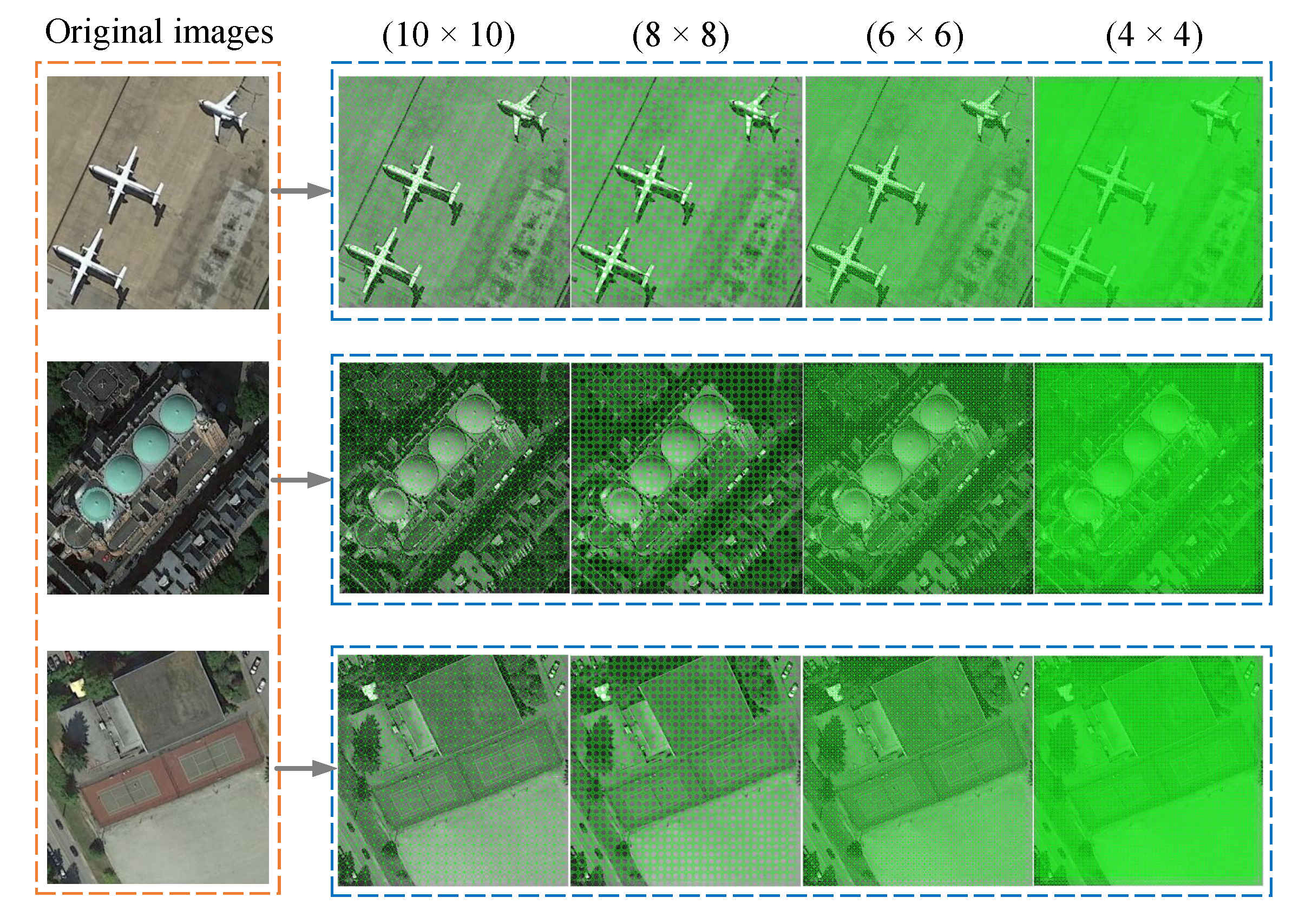
In general, patch sampling or feature learning is a critical component for building up an intelligent system either for the CNN model or BoW-based approaches. Ideally, special attention should be paid to image patches that are the most informative for the classification task. This is due to the fact that objects can appear at any location in the image [24]. Recent studies address this issue by sampling feature points based on a regular dense grid [25] or a random strategy [26] because there is no clear consensus about which sampling strategy is most suitable for natural scene images. Although multiscale keypoint detectors (e.g., Harris-affine, Laplacian of Gaussian) as samplers [27] are well studied in the computer vision community, they were not designed to find the most informative patches for scene image classification [26]. In this paper, instead of working towards a new CNN model or a local descriptor, we introduce a patch-based discriminative learning (PBDL) to extract image features region by region based on small, medium, and large neighborhood patches to fully exploit the spatial structure information in the BoW model. Here, the definition of different neighborhood sizes is considered small, medium, or large regions depending on the patch sizes. For instance, the patch size $(4\times 4)$ represents the small region, the patch size $(6\times 6)$ represents the medium region, and large sizes are represented by $(8\times 8)$, $(10\times 10)$. This is motivated by the fact that different patch sizes still exhibit good learning ability of spatial dependencies between image region features that may help to interpret the scene [28,29]. Figure 2 illustrates the extracted regions used in our work. In Figure 2 from right to left: the first column images represent the dark green color due to the patch size of $(4\times 4)$. The images in the second column show the SURF features with the size of $(6\times 6)$. Likewise, $(8\times 8)$, and $(10\times 10)$ patch sizes are used, and their features are displayed in the third and fourth columns, respectively. Moreover, the proposed method also magnifies the visual information by utilizing Gaussian pyramids in a scale-space setting to improve the classification performance. In particular, the idea of magnifying the visual information in our work is based on generating a multi-scale representation of an image by creating a one-parameter family of derived signals [30]. Since the proposed multi-level learning is based on different image patch sizes, spatial receptive fields may overlap due to unique nature of remote sensing scene images (e.g., buildings, fields, etc.). Thus, we also consider the sampling redundancy problem to minimize the presence of nearby or neighboring pixels. We show that overlapping pixels can be minimized by setting pixel stride equal to the pixel width of the feature window.

Next, we balance the contribution of individual patch features by proposing a simple fusion strategy based on two motivations. Firstly, the proposed method introduces a simple fusion strategy that can surpass the previous performance without utilizing state-of-the-art fusion methods such as DCA [32], PCA [33], CCA [34], as previously utilized in remote sensing domain (we further discuss this aspect in Section 4.3). The second motivation is to evade the disadvantages of traditional dimensionality reduction techniques such as principle component analysis (PCA) because of their data-dependent characteristic, the computational burden of diagonalizing the covariance matrix, and the lack of guarantee that distances in the original and projected spaces are well retained. Finally, the BiLSTM [35] network is adopted after combining small, medium, and large scale spatial and visual histograms to classify scene images. We demonstrate that the collaborative fusion of the different regions (patch sizes) addresses the problem of intra-class difference, and the aggregated multi-scale features in scale-space pyramids can be used to solve the problem of inter-class similarity. To this end, our main contributions in this paper are summarized as follows:

1.

We present a patch-based discriminative learning to combine all the surrounding features into a new single vector and address the problem of intra-class diversity and inter-class similarity.

2.

We demonstrate the effectiveness of patch-based learning in the BoW model for the first time. Our method suggests that exploring visual descriptor on image regions independently can be more effective than random sampling for the remote sensing scene classification.

3.

To enlarge the visual information, smoothing and stacking is performed by convolving the image with Gaussian second derivatives. In this way, we integrate the fixed regions (patches) into multiple downscaled versions of the input image in a scale-space pyramid. By doing so, we explore more content and important information.

4.

The proposed method not only surpasses the previous BoW methods but also several state-of-the-art deep-learning-based methods on four publicly available datasets and achieves state-of-the-art results.

The rest of this work is organized as follows. Section 2 discusses the related literature work of this study. Section 3 introduces the proposed PBDL for remote sensing scene classification. Section 4 shows the experimental results of the proposed PBDL on several public benchmark datasets. Section 5 summarizes the entire work and gives suggestions for future research.

2. Literature Review

In the early 1970s, most of the early methods in remote sensing image analysis focused on per-pixel analysis, through labeling each pixel in the satellite images (such as the Landsat series) with a semantic class, because the spatial resolution of Landsat images acquired by satellite sensor is very low where the size of a pixel is close to the sizes of the objects of interest [7]. With the advances in remote sensing technology, the spatial resolution of remote sensing images is increasingly finer than the typical object of interest, and the objects are usually composed of many pixels, such that single pixels lost their semantic meanings. In such cases, it is difficult or sometimes impoverished to recognize scene images at the pixel level solely. In 2001, Blaschke and Strobl [36] raised the critical question “What’s wrong with pixels?” to conclude that analyzing remote sensing images at the object level is more efficient than the statistical analysis of single pixels. Afterward, a new paradigm of approaches to analyze remote sensing images at the object level has dominated for the last two decades [7].

However, pixel and object-level classification methods may not be sufficient to always classify them correctly because pixel-based identification tasks carry little semantic meanings. Under these circumstances, semantic-level remote sensing image scene classification seeks to classify each given remote sensing image patch into a semantic class that contains explicit semantic classes (e.g., commercial area, industrial area, and residential area). This led to categorization of remote sensing image scene classification into three main classes according to the employed features: human engineering-based methods, unsupervised feature learning (or global-based methods), and deep feature learning-based methods. Early works in scene classification required a considerable amount of engineering skills and are mainly based on handcrafted descriptors [8,10,37,38]. These methods mainly focused on texture, color histograms, shape, spatial and spectral information, and were invariant to translation and rotation.

In brief, handcrafted features have their own benefits and disadvantages as well. For instance, color features are more convenient to extract in comparison with texture and shape features [38]. Indeed, color histograms and color moments provide discriminative features and can be computed based on local descriptors such as local binary patterns (LBPs) [8], scale invariant feature transform (SIFT) [9], color histogram [10], and histogram oriented gradients (HOG) [11]. Although color-based histograms are easy to compute, they do not convey spatial information and the high resolution of scene images makes it very difficult to distinguish the images with the same colors. Yu et al. [39] proposed a new descriptor called color-texture-structure (CTS) to encode color, texture, and structure features. In their work, a dense approach was used to build the hierarchical representation of the images. Next, the co-occurrence patterns of regions were extracted and the local descriptors were encoded to test the discriminative capability. Tokarczyk et al. [38] proposed to use the integral images and extract discriminative textures at different scale levels of scene images. The features were named Randomized Quasi-Exhaustive (RQE) which are capable of covering a large range of texture frequencies. The main advantage of extracting these spatial cues such as color, texture, or spatial information is that they can be directly utilized by classifiers for scene classification. On the other hand, every individual cue focused only on one single type of feature, so it remains challenging or inadequate to illustrate the content of the entire scene image. To overcome this limitation, Chen et al. [37] proposed a combination of different features such as color, structure, and texture features. To perform the classification task, the k-nearest-neighbor (KNN) classifier and the support vector machine classifiers (SVM) were employed and the decision level fusion was performed to improve the performance of scene images. Zhang et al. [40] focused on the variable selection process based on random forests to improve land cover classification.

To further improve the robustness of handcrafted descriptors, the bag-of-words (BoW) framework has made significant progress for remote sensing image scene classification [41]. By learning global features, Khan et al. [42] investigated multiple hand-crafted color features in the bag-of-word model. In their work, color and shape cues were used to enhance the performance of the model. Yang et al. [43] utilized the BoW model using the spatial co-occurrence kernel, where two spatial extensions were proposed to emphasize the importance of spatial structure in geographic data. Vigo et al. [44] proved that incorporating color and shape in both feature detection and extraction significantly improves the bag-of-words based image representation. Sande et al. [45] proposed a detailed study about the invariance properties of color descriptors. They concluded that the addition of color descriptors over SIFT increases the classification accuracy by 8%. Lazebnik et al. [14] proposed a spatially hierarchical pooling stage to form the spatial pyramid method (SPM). To improve the SPM pooling stage, sparse codes (SC) of SIFT features were merged into the traditional SPM [46]. Although, researchers have proposed several methods to achieve good performance for land use classification, especially compared to handcrafted feature-based methods, one of the major disadvantages of BoW is that it neglects the spatial relationships among the patches, and the performance remains unclear, especially the localization issue is not well understood.

Recently, most of the current state-of-the-art approaches generally rely on end-to-end learning to obtain good feature representations. Specifically, the use of convolutional neural networks (CNN) is the state-of-the-art framework in scene image classification. In this case, convolutional layers convolve the local image regions independently, and pass their results to the next layer, whereas pooling layers summarize the dimensions of data. Due to the wide range of image resolution and the various scales of detail textures, fixed-sized kernels are inadequate to extract scene features of different scales. Therefore, the focus of current literature has been shifted to multi-scale and fusion methods in the scene image classification domain, and existing deep learning methods are making full use of multi-scale information and fusion for a better representation. For instance, Ghanbari et al. [47] proposed a multi-scale method called dense-global-residual network to reduce the loss of spatial information and enhance the context information. The authors used a residual network to extract the features and a global spatial pyramid pooling module to obtain dense multi-scale features at different levels. Zuo et al. [48] proposed a convolutional recurrent neural network to learn the spatial dependencies between image regions and enhance the discriminative power of image representation. The authors trained their model in an end-to-end manner where CNN layers were used to generate mid-level features and RNN was used for learning contextual dependencies. Huang et al. [49] proposed an end-to-end deep learning model with multi-scale feature fusion, channel-spatial attention, and a label correlation extraction module. Specifically, a channel-spatial attention mechanism was used to fuse and refine multi-scale features from different layers of the CNN model.

Li et al. [50] proposed an adaptive multi-layer feature fusion model to fuse different convolutional features with feature selection operation, rather than simple concatenation. The authors claimed that their proposed method is flexible and can be embedded into other neural architectures. Few-shot scene classification was introduced by proposing an end-to-end network, called discriminative learning of adaptive match network (DLA-MatchNet) in [51]. The authors addressed the issues of the large intraclass variances and interclass similarity by introducing the attention mechanism into the feature learning process. In this way, discriminative regions were extracted, which helps the classification model to emphasize valuable feature information. Xiwen et al. [52] proposed a unified annotation framework based on a stacked discriminative sparse autoencoder (SDSAE) and weakly supervised feature transferring. The results demonstrated the effectiveness of weakly supervised semantic annotation in remote sensing scene classification. Rosier et al. [53] found that fusing Earth observation and socioeconomic data lead to increases in the accuracy of urban land use classification.

Due to the wide range of image resolution and various scales of detail textures, fixed-sized CNN kernels are inadequate to extract scene features of different scales. Therefore, the focus has been shifted to multi-scale, attention mechanism, and fusion methods in the scene image classification domain, and existing deep learning methods are making full use of multi-scale information and fusion for a better representation. The main idea behind the attention mechanism was initially developed in 2014 for natural language processing applications [54] based on the assumption that different weights assigned to different pieces of information can be provided to attract the attention of the model [24].

In our work, we pay particular attention to the previous work [33] where the authors claimed that a simple combination strategy achieves less than $1\%$ accuracy when the fusion of deep features (AlexNet, VGG-M, VGG-S and CaffeNet) was applied. Thus, a natural question arises: can we combine different region features effectively and efficiently to address scene image classification? With the exception [32], to our knowledge, this question still remains mostly unanswered. In particular, the deep features from fully connected layers with the DCA method were fused to improve the scene image classification in [32]. We show that raw SURF features produce good informative features to describe the images scene with a simple concatenation of different patch-size features. Experimental results on four public remote sensing image datasets demonstrate that combining the proposed discriminative regions can improve performance up to $20\%$, $15\%$, $10\%$ and $6\%$ for NWPU, AID, WHU-RS and UC Merced datasets, respectively.

3. The Proposed Method

The proposed approach is divided into four indispensable components: (a) estimation of patch-based regions (b) scale-space representation (c) information fusion and (d) a Recurrent neural network for classification purpose. We first describe the procedure of patch-based learning. Next, we describe the proposed fusion along the classification process of BiLSTM network. The overall procedure of the proposed approach is illustrated in Figure 3.

3.1. Estimation of Patch-Based Regions

To explore the spatial relationship between scenes or sub-scenes, we propose to extract multi-level features assuming that different regions contain discriminative characteristics that can be used to extract more meaningful information. Based on our observation, the size of the neighborhood has a great impact on the scene representations and classification performance. To demonstrate this, we first define a region over the entire image, where the small $(4\times 4)$, medium $(6\times 6)$, and larger $(8\times 8)$, $(10\times 10)$, patch sizes are used, and each patch is then processed individually. In particular, given an image $I:\Omega ⟼R^Q$ where $\Omega =\left\{0,1,\dots ,G-1\right\}\times \left\{0,1,\dots ,H-1\right\}$, G and H represent the number of rows and columns of an image, respectively. The sampling patch g is the number of sampled grids divided by the number of pixels in an image; the objective is to determine a subset D of $\Omega$ for a given sampling patch g, such that:

$$\begin{array}{c}\hfill D=\left\{\left.c\right|cϵ\Omega ,j\left(x\right)isinformative,\frac{\#C}{G\times H}=g\right\}\end{array}$$

(1)

where c denotes the local patches (i.e., grids) defined at the image pixel x, $j\left(x\right)$ is the response map at x and $\#C$ represents the number of grids. In our work, we set the size of the sampling patch g to the number of sampled patches partitioned by the number of pixels in an image. Therefore, an image is represented by the same number of patches that defines the representative area of the same size. Thus, four kinds of grid sampling size $\left(g\right)$ as mentioned above were used for each image to ensure that the output is a good representative of the information content.

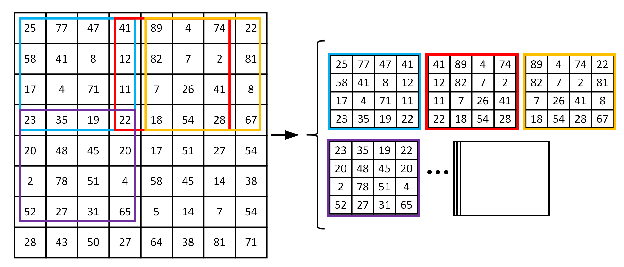
Moreover, we adopt a multi-scale representation by utilizing different scale $\sigma$ sizes. However, the natural question is whether the large scale images can provide salient features from every scale $\sigma$, or, equivalently, whether small scaled images are enough for the classifier. For instance, taking an equal $4\times 4$ pixel stride at the scale $\sigma =1.6$, should the proposed sampling at a 4 pixel stride be able to recognize objects at a wide variety of scales? This is an open question that must be addressed during feature extraction stage. Recent studies generally address this issue by sampling the feature points either uniformly or randomly [55,56]. For uniform sampling, local patches are sampled densely within regular sampling grids across an image with certain pixel spacing. For instance, an example image with the neighborhood patch $(4\times 4)$ size is provided in Figure 4 to show how the local descriptor can be exploited using a fixed-size window with a constant stride 1. Such an approach would be sub-optimal if:

• There is not much spatial information available at the larger scales. This suggests that larger scales should not be weighted equally.
• A large number of scale images provide more redundancy at the same pixel stride. Since the fixed pixel stride can share overlapping, spatial closeness must be taken into account before employing the local descriptor.

Perhaps surprisingly, the proposed strategy has the potential to be more efficient, exploring the salient features at a wide variety of scales. Specifically, if the proposed sampling uses a 4 pixel strides for $\sigma =1.6$, then it would also utilize other pixel stride of 6, 8 and 10 for higher scales $\sigma =6.0$ to avoid ambiguity. Thus, the proposed sampling method overcome the overlapping or redundancy problem by, first, setting the different patch regions, e.g., $(4\times 4)$, $(6\times 6)$, $(8\times 8)$, $(10\times 10)$, and then keeping the pixel stride equal to the pixel width of the feature window (i.e., 4, 6, 8 and 10). By doing this, a bias, if it exists at all, would then only be applicable at the borders of such a region, but not for the central pixels (we further discuss this argument in Section 4.3).

3.2. Scale-Space Representation

To achieve multi-scale information of each region, we propose to use multi-scale filtering motivated by the fact that it can adaptively integrate the edges of small and large structures referring as image pyramids. Inspired by the Gaussian scale-space theory [57], Hessian matrix-based extractor is used by enlarging the size of the box filter without compromising on the size of the original image. In this way, multi-scale information could be achieved based on a second derivative Gaussian filter and a convolution operation as follows, see (Equations (2) and (3)):

$$\begin{array}{c}\hfill H(X,\mu )=\left[\frac{L_{xx}(X,\mu ),L_{xy}(X,\mu )}{L_{xy}(X,\mu ),L_{yy}(X,\mu )}\right]\end{array}$$

(2)

$$\begin{array}{c}\hfill L_{xx}(X,\mu )=I(x,y)\times \frac{{\partial }^2}{\partial x^2}g\left(\mu \right)\end{array}$$

(3)

where $L_{xx}(X,\mu )$ represents a second-order differentiated Gaussian filter along the $xx$ direction while $L_{xy}(X,\mu )$ and $L_{yy}(X,\mu )$ denotes second order differentiated Gaussian filters and convolution operations in $xy$ direction (diagonal) and $yy$ direction (vertical), respectively [58]. Since the Gaussian filter has a drawback due to a large amount of computation, this issue is addressed by using box filters [31] which have been particularly employed for fast implementation such as:

$$\begin{array}{c}\hfill det\left(H_{app}\right)=D_{xx}{D}_{yy}-{\left(\lambda D_{xy}\right)}^2\end{array}$$

(4)

where $\lambda$ required to balance the Hessian determinant and is acquired using the Frobenius Norm. In this way, computation amount can be significantly decreased as:

$$\begin{array}{c}\hfill \lambda =\frac{{\left|L_{xy}(1,2)\right|}_F{\left|D_{yy}\left(9\right)\right|}_F}{{\left|L_{yy}(1,2)\right|}_F{\left|D_{xy}\left(9\right)\right|}_F}=0.912\cong 0.9\end{array}$$

(5)

Hence, the proposed idea takes the advantage of a hybrid feature extraction scheme, i.e., multi-scale interest points and dense sampling, where we start from a dense sampling on regular grids with the repeatability of interest points at multiple scales. Figure 5 displays the dense sampling, sparse interest points, and hybrid (dense interest points) scheme. Once the scale space has been built, we utilize SURF descriptor [31] to extract the features within a bounded search area. For an image I, image scales $m_i=(i=1,2,\dots ,n)$ are denoted as $x_{mi}=(i=1,2,\dots ,n)$. Formally, for each smoothed image, the feature extracted from the SURF is illustrated as follows:

$${\mathit{f}}_{m_i}=SURF\left(x_{mi}\right),i=1,2,\dots ,n$$

(6)

where n is the number of scales, i is the index of scale, $x_{mi}$ is the $i^{th}$ scale, $x_{mi}$ is the region at $i^{th}$ scale, and ${\mathit{f}}_{mi}$ is the SURF feature for $x_{mi}$.

In order to construct the visual vocabulary, we use the BoW framework that produced a histogram through a quantization of feature space using K-means clustering. The optimal value for K remains challenging and we select it according to the size of the dataset by trial-and-error learning. The histogram becomes a final representation of the image.

3.3. Information Fusion

Information fusion is the process of combining multiple pieces of information to provide more consistent, accurate, and useful information than a single piece of information. In general, it is divided into four categories: decision level, scale level, feature level, and pixel-level [59]. Among them, feature-level fusion has comparatively a shorter history but is an emerging topic in remote sensing domain. The spatial relation between the proposed regions can improve scene classification in two aspects. First, aggregating the information of a neighborhood and its adjacent neighborhoods assists in recognizing the features that accurately represent the scene type of the image. For instance, determining whether farmland belongs to a forest field or a meadow requires information about its neighboring area. Second, the natural relationship of the spatial distribution pattern of a scene helps us to infer the scene category. An industrial area, for instance, is likely planar, and the runway is always linear. Therefore, we select to combine four different regions based on multiscale features, with the aim to obtain more informative and relevant features to represent the input image. Each input image I produced four sets of a histogram of visual words, which are generated by different pixel strides through the k-means clustering process as previously mentioned and denoted as $Q_1$, $Q_2$, $Q_3$, and $Q_4$. Specifically, the first set of histogram of visual words extracted from the image is $Q_1=(q_{e_1},q_{e_2},\dots ,q_{e_n})\in R^z$; $R^z$ represents the z-dimensional vector. The second set is represented as $Q_2=(q_{w_1},q_{w_2},\dots ,q_{w_n})\in R^w$; $R^w$ represents the w-dimensional vector. $Q_1$ and $Q_2$ are the outputs of two different patch sizes. Similarly, the third and fourth sets are represented as $Q_3=(q_{y_1},q_{y_2},\dots ,q_{y_n})\in R^y$; $R^y$ represents the y-dimensional vector, and $Q_4=(q_{u_1},q_{u_2},\dots ,q_{u_n})\in R^u$; $R^u$ represents the u-dimensional vector, respectively. Information fusion is performed by the concatenation of $Q_1$,$Q_2$,$Q_3$ and $Q_4$, and the result is denoted by $Q_f$, which corresponds to an $(z+w+y+u)$-dimensional vector. Thus, the fusion operation is achieved by the following formula:

$$Q_f=Q_1\oplus Q_2\oplus Q_3\oplus Q_4,Q_f\in R^{z+w+y+u}$$

(7)

where the elements $(q_{e_1},q_{e_2},\dots ,q_{e_n})$ of $Q_1$, the elements $(q_{w_1},q_{w_2},\dots ,q_{w_n})$ of $Q_2$, the elements $(q_{y_1},q_{y_2},\dots ,q_{y_n})$ of $Q_3$, and the elements of $(q_{u_1},q_{u_2},\dots ,q_{u_n})$ of $Q_4$ construct a new vector $Q_f$ to express the fused feature vector.

3.4. Recurrent Neural Network (RNN)

The extracted multilevel and multiscale features are used as spatial sequences and fed to a bidirectional long short-term memory (BiLSTM) [35] to capture the long-range dependency and contextual relationship. In particular, the BiLSTM was used to exploit the spatial dependency of features and automatically find the optimal combination through gates mechanism. BiLSTM determines the input sequence $i=i_1,i_2,\dots ,i_n$ from the opposite order to a forward hidden sequence $\overrightarrow{{\mathrm{f}}_{\mathrm{t}}}=(\overrightarrow{{\mathrm{f}}_1},\overrightarrow{{\mathrm{f}}_2},\dots ,\overrightarrow{{\mathrm{f}}_{\mathrm{n}}})$ and a backward hidden sequence $\overleftarrow{{\mathrm{f}}_{\mathrm{t}}}=(\overleftarrow{{\mathrm{f}}_1},\overleftarrow{{\mathrm{f}}_2},\dots ,\overleftarrow{{\mathrm{f}}_{\mathrm{n}}})$. The encoded vector $v_t$ is computed by the accumulation of the final forward and backward outputs $v_t=[\overrightarrow{{\mathrm{f}}_{\mathrm{t}}},\overleftarrow{{\mathrm{f}}_{\mathrm{t}}}]$.

$$\begin{array}{c}\hfill \overrightarrow{{\mathrm{f}}_{\mathrm{t}}}=\delta (W_{\overrightarrow{\mathrm{f}}i}{i}_t+W_{\overrightarrow{\mathrm{f}}\overrightarrow{\mathrm{f}}}{\overrightarrow{\mathrm{f}}}_{t-1}+q_{\overrightarrow{\mathrm{f}}}),\end{array}$$

(8)

$$\begin{array}{c}\hfill \overleftarrow{{\mathrm{f}}_{\mathrm{t}}}=\delta (W_{\overleftarrow{\mathrm{f}}i}{i}_t+W_{\overleftarrow{\mathrm{f}}\overleftarrow{\mathrm{f}}}{\overleftarrow{\mathrm{f}}}_{t+1}+q_{\overrightarrow{\mathrm{f}}}),\end{array}$$

(9)

$$\begin{array}{c}\hfill v_t=W_{v\overrightarrow{\mathrm{f}}}\overrightarrow{{\mathrm{f}}_{\mathrm{t}}}+W_{v\overleftarrow{\mathrm{f}}}\overleftarrow{{\mathrm{f}}_{\mathrm{t}}}+q_v\end{array}$$

(10)

where $\delta$ is the logistic sigmoid function and $v=(v_1,v_2,\dots v_t\dots ,v_n)$ is the output sequence of the first hidden layer.

4. Datasets and Experimental Setup

In this section, we first provide a brief description of the four databases that are used to test and evaluate our method. Then, the implementation details and ablation analysis are discussed and the results are compared with other state-of-the-art methods.

4.1. Datasets

UC Merced Land Use Dataset (UC-Merced): This dataset was obtained from the USGS National Map Urban Area with a pixel resolution of one-foot [43]. It contains 21 distinctive scene categories and each class consists of 100 images of size $256\times 256\times 3$. Inter-class similarity, for example, highway and architecture scenes can be easily mixed with other scenes, such as freeways and buildings, which makes this dataset a challenging one.

WHU-RS Dataset: It was collected from satellite images of Google Earth [60]. This dataset consists of 950 scene images and 19 classes with a size of $600\times 600$. Each image varies greatly in high resolution, scale, and orientation, which makes it more complicated than the UCM dataset.

Aerial Image Dataset (AID): There are $10,000$ images in AID dataset, which are categorized into 30 scene classes [6]. Each class contains images ranging from 220 up to 420 with the fixed size of $600\times 600$ pixels in the RGB space. The pixel resolution changes from about 8 m to about half a meter.

NWPU-RESISC45 Dataset: It consists of 31,500 remote sensing images divided into 45 scene classes, covering more than 100 countries and regions all over the world [61]. Each class contains 700 images with the size of $256\times 256$ pixels. This dataset is acquired from Google Earth (Google Inc., Mountain View, CA, USA), where the spatial resolution varies from 30 to 0.2 m per pixel. This is one of the largest datasets of remote sensing images and is 15 times larger than the most widely-used UC Merced dataset. Hence, the rich image variations, high inter-class similarity, and the large scale make the dataset even more challenging.

4.2. Implementation Details

To evaluate the performance on the above-mentioned datasets, the BoW was used as the base architecture with four distinct image regions and seven adjacent Gaussian scaled images, i.e., $[1.6,2.5,3.5,4.5,5.5,6.0,6.4]$. The vocabulary size of k in the remote sensing domain varies from a few hundred to thousands. We set the size of visual vocabulary to $15,000$ for UC Merced, AID, NWPU, and $10,000$ for the WHU-RS dataset. The results of all the experiments reported in our work use a $20\%$ training ratio for NWPU, $50\%$ for AID, and $80\%$ for UC Merced and WHU-RS datasets. The BiLSTM is trained using the Adam optimizer with a gradient threshold 1, while the minibatch size of 32 with a hidden layer dimension of 80. For the UC Merced dataset, a hidden layer dimension of 100 was used. Initializing the BiLSTM with the right weights is a challenging task because the standard gradient descent from random initialization can hamper the training of BiLSTM. Therefore, we set the recurrent weights with Glorot initializer (Xavier uniform) [62] which performs the best in all scenarios of our experiments. To decrease the computation complexity and overfitting risk on AID and NWPU datasets, we empirically set four Gaussian scaled images, i.e., $[1.6,2.5,3.5,4.5]$.

4.3. Ablation Study

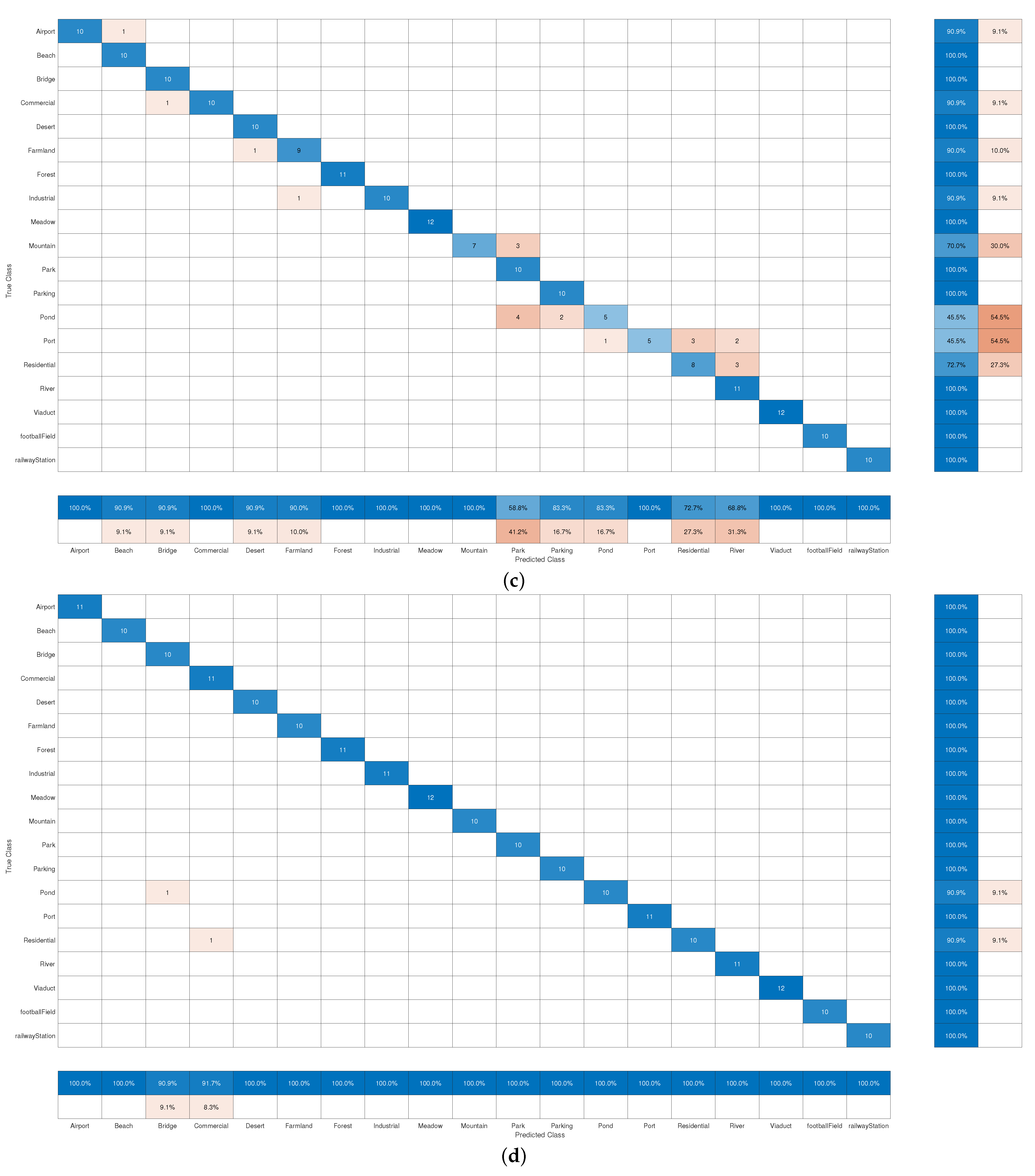
We thoroughly validate the performance of each neighborhood size by performing an ablation study. In

Table 1. Patch-based analysis on each dataset.

	Different Neighborhood Combinations	Accuracy (%)
UC Merced dataset
1	$4\times 4$	88.10
2	$6\times 6$	86.79
3	$8\times 8$	85.43
4	$10\times 10$	84.52
WHU-RS dataset
1	$4\times 4$	86.10
2	$6\times 6$	88.70
3	$8\times 8$	91.52
4	$10\times 10$	89.52
NWPU-RESISC45 dataset
1	$4\times 4$	67.10
2	$6\times 6$	65.61
3	$8\times 8$	64.52
4	$10\times 10$	62.52
AID dataset
1	$4\times 4$	75.60
2	$6\times 6$	77.13
3	$8\times 8$	78.52
4	$10\times 10$	76.90

, we have reported the results of estimating PBDL on UC Merced, WHU-RS, NWPU, and AID datasets. Our one-stage detection method on the WHU-RS dataset with the neighborhood size of $(4\times 4)$ achieves $86.10\%$ accuracy and the numerical results of each category are shown in Figure 6a. The diagonal elements represent the number of images for which the classifier predicted correctly. It can be seen that several classes such as bridge (three images), pond (six images), farmland (three images), residential (three images), and viaduct (two images) are misclassified. In Figure 6b, we show that when the neighborhood size $(10\times 10)$ increases, the overall classification is improved from $86\%$ to $89\%$, which is $3\%$ higher than the $(4\times 4)$ size. After combining both kinds of features, we notice that images of the bridge, pond, farmland, and residential are predicted correctly up to $99\%$ and achieve an overall classification accuracy of $95\%$ as shown in Figure 6c. The final results are obtained by combining all the neighborhood features and are displayed in Figure 6d. A significant improvement can be observed in overall classification performance and only two images are found misclassified in the WHU dataset. Based on these results, we conclude that a single BoW model cannot provide state-of-the-art results without aggregating the features of discriminative regions. From the findings of

Table 2. The general comparison of the proposed method after information fusion in terms of accuracy (%), training and testing time per second.

Dataset	Patch-Based Fusion	Accuracy	Training (s)	Testing (s)
UC-Merced	BoW(1+2)+BiLSTM	94.10	8671.74	253.16
	BoW(1+2+3)+BiLSTM	97.76	15,007.61	480.74
	BoW(1+2+3+4)+BiLSTM	99.57	19,343.48	601.32
WHU-RS	BoW(1+2)+BiLSTM	95.49	10,452.38	676.3
	BoW(1+2+3)+BiLSTM	98.20	17,678.57	1104.5
	BoW(1+2+3+4)+BiLSTM	99.63	22,904.76	1452.6
NWPU	BoW(1+2)+BiLSTM	89.32	21,271.08	7798.06
	BoW(1+2+3)+BiLSTM	94.72	32,906.62	12,695.59
	BoW(1+2+3+4)+BiLSTM	97.13	44,542.16	16,594.12
AID	BoW(1+2)+BiLSTM	92.77	40,035.02	9131.96
	BoW(1+2+3)+BiLSTM	96.51	62,152.53	14,697.94
	BoW(1+2+3+4)+BiLSTM	98.43	82,170.04	19,263.92

, it is evident that the BoW(1+2)+BiLSTM yields good performance on the UC Merced dataset right from the start. When we integrate the features of different neighborhood(1+2+3) sizes, the model further improves the performance up to $9\%$ than the single grid-sized BoW model. By combining all the neighborhood features, we achieved the best performance i.e., $99\%$. Similarly, for NWPU and AID datasets, a significant difference can be seen even with combining two neighborhood(1+2) sizes, and the performance is boosted when increasing the number of neighborhood(1+2+3) sizes, surpassing $90\%$ with just $10\%$ of all samples as a training sample. In addition, UC-Merced, WHU-RS, NWPU, and AID datasets take 19,343.48 s, 22,904.76 s, 44,542.16 s, and 82,170.04 s for training, and 601.32 s, 1452.6 s, 1452.6 s, and 19,263.92 s for testing, respectively. One can observe that the size of the patch has a significant influence in the time consuming of the visual vocabulary-based method. Although the time required to construct the vocabulary is in the range of few hours, the methods provide acceptable classification performance. Thus, the results demonstrate that the different neighborhood sizes play different roles in classifying remote sensing scene images, and the proposed patch-based discriminative learning plays an essential role in significantly improving the feature representation for remote sensing scene classification.

4.3.1. Scale Factor of Gaussian Kernel

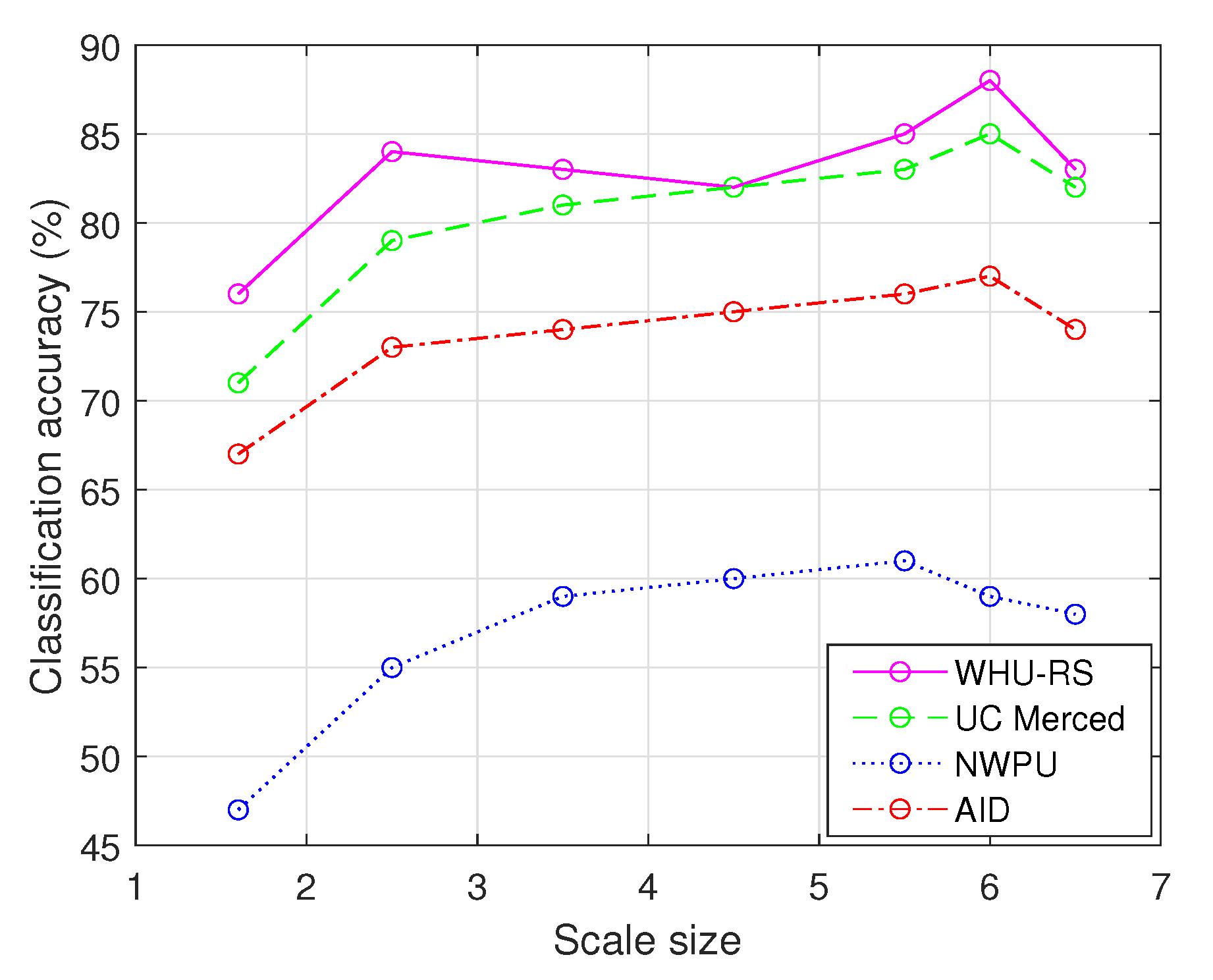
Figure 7 shows the classification performance of each scaled image based on $10\times 10$ neighborhood size. The PBDL extracts multi-scale dense features according to the scale factor to control the Gaussian kernel. It can be observed that with the increase of scale $\sigma$ factor, the performance first improves and then gradually decreases after the $\sigma =6.0$ scaled image. We conclude that including a certain range of Gaussian smoothed images can improve the performance, but too many of them not only reduce details but also degrade the performance.

4.3.2. Codebook Learning

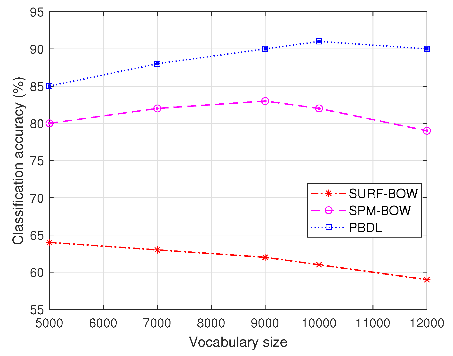
We quantitatively analyzed the performance with the SURF descriptor and standard SPM method in the bag-of-words framework. An engaging question is how much the performance can be improved by defining the proposed spatial locations with multi-scale information. With this in mind, we set different vocabulary sizes for WHU-RS dataset. The respective outcomes can be found in Figure 8. One can see that even the proposed one-stage detection method with the neighborhood size of $(4\times 4)$ significantly outperforms the SPM method with the vocabulary size of 10,000. Similarly, using the SURF descriptor in the BoW framework cannot achieve the best performance and even provided more than $20\%$ lower accuracy than ours. The training ratio was set to $80\%$ in order to conduct the experiments. Thus, we investigated the importance of the role played by the vocabulary size and concluded that an extremely large vocabulary size can decrease the model performance.

4.3.3. Quantitative Comparison of Different Fusion Methods

Table 3. Comparison of classification accuracy (%) with feature-level fusion methods under different training sizes on the WHU-RS dataset.

Train Data	DCA [32]	PCA [33]	CCA [34]	Ours
30%	93.72 ± 0.34	92.13 ± 0.32	92.88 ± 0.51	94.13 ± 0.32
40%	94.13 ± 0.11	93.88 ± 0.41	94.11 ± 0.61	95.41 ± 0.59
50%	96.82 ± 0.55	94.52 ± 0.22	95.22 ± 0.43	97.05 ± 0.41

provides a quantitative analysis based on the different sizes of the training data. All the compared methods such as [32,33,34] performed feature-level fusion based on discriminant correlation analysis (DCA), principal component analysis (PCA), or canonical correlation analysis (CCA) to improve the scene classification performance. For instance, the authors in [32] fused the deep neural network features based on DCA. To make the deep learning features more discriminant, features of different models were combined based on PCA in [33]. The global features under the BoW framework were fused based on CCA in [34]. In comparison with these state-of-the-art fusion methods, our proposed fusion performs best even with the size of $30\%$ sampling ratio.

4.3.4. Performance Comparison of Different Pixel Strides

During patch-based learning, we consider the problem of sampling redundancy. Although different number of image patch sizes have been used in a traditional dense feature sampling approach, the optimal pixel strides are not deeply investigated in the literature. We show that same pixel stride $\left(4\right)$ corresponding to the pixel width of the feature window $(4\times 4)$ is better suited to the domain of remote sensing scene image classification. In this way, it allows the classifiers to consider more scales with minimal increase in overlapping or redundancy.

Table 4. Comparison of classification accuracy (%) based on different pixel strides (PS) with WHU-RS dataset. The PS1 and PS2 are corresponding to pixel stride 1 and 2. The PS represents the pixel stride equal to the patch size (4).

Dataset	PS1	PS2	PS
WHU-RS	95.54 ± 0.52	97.94 ± 0.47	99.63 ± 0.21

shows the impact of this effective parameter tuning. The PS represent the same pixel stride corresponding to the proposed patch sizes while pixel stride 1 and 2 are used for comparison purpose and expressed as PS1 and PS2, respectively. One can see that this basic modification provides improved results on all datasets and minimized the overlapping in (x,y) space. In addition, Figure 9 visualizes the point of redundancy.

4.3.5. Visualization of Feature Structures

One of the advantages of the proposed approach is that we can interpret the classification process of the model. Especially for each stage, we can see how the features are structured into the data space as well as their impact with respect to the different classification stages. Taking this into consideration, we employed the “t-distributed stochastic neighboring embedding” (t-SNE) algorithm [63] and illustrated the derived embeddings into three separated processing stages: (1) one-stage learning, (2) combined learning (PBDL), and (3) BiLSTM classified features for the WHU dataset. The features with the patch size of $4\times 4$ in Figure 10a show that the most classes are strongly correlated, which makes the classifier (BiLSTM) hard to separate them. We also visualize the clusters by fusing all the neighborhood features in Figure 10b. The derived clusters indicate that the proposed fusion reduces the correlation between similar classes and can capture more variability in the feature space. Moreover, it could be noticed from Figure 10c that all the classes are well separable which could potentially lead to a better performance when training BiLSTM on remote sensing dataset.

4.4. Performance Comparison with State-Of-The-Art Methods

4.4.1. NWPU-RESISC45 Dataset

To demonstrate the superiority of the proposed method, we evaluated the performance against several state-of-the-art classification methods on the NWPU dataset as shown in

Table 5. Classification accuracy (%) for the NWPU dataset with two training ratios.The results are obtained directly from the corresponding papers.

Method	10%	20%
BoW with dense SIFT [64]	41.72 ± 0.21	44.97 ± 0.28
BOCF [64]	82.65 ± 0.31	84.32 ± 0.17
BoVW+SPM [61]	27.83 ± 0.61	32.96 ± 0.47
D-CNN [65]	89.22 ± 0.50	91.89 ± 0.22
Triple networks [66]	-	92.33 ± 0.20
MDFR [67]	83.37 ± 0.26	86.89 ± 0.17
APDC-Net [68]	85.94 ± 0.22	87.84 ± 0.26
BoWK [34]	-	66.87 ± 0.90
SFCNN [69]	89.89 ± 0.16	92.55 ± 0.14
Attention GANs [70]	86.11 ± 0.22	89.44 ± 0.18
MDFR [67]	83.37 ± 0.26	86.89 ± 0.17
CNN + GCN [23]	90.75 ± 0.21	92.87 ± 0.13
Color fusion [71]	-	87.50 ± 0.00
Graph CNN [72]	91.39 ± 0.19	93.62 ± 0.28
AlexNet+SAFF [73]	80.05 ± 0.29	84.00 ± 0.17
VGG-VD16+SAFF [73]	84.38 ± 0.19	87.86 ± 0.14
IDCCP [74]	91.55 ± 0.16	93.76 ± 0.12
SEMSDNet [75]	91.68 ± 0.39	93.89 ± 0.63
MFST [76]	92.64 ± 0.08	94.90 ± 0.06
T-CNN [77]	90.25 ± 0.14	93.05 ± 0.12
PBDL (The proposed)	94.20 ± 0.81	97.13 ± 0.92

. Especially, we choose mainstream BoW and deep-learning-based methods and compared the performance of scene classification. It could be observed from Table 5, that the proposed approach, by combining all neighborhood-based features, achieved the highest overall performance of $94.20\%$ and $97.13\%$ using $10\%$ and $20\%$ training ratios, respectively. Likewise, NWPU is found to be much more difficult than the other three datasets and our proposed method outperforms the previous state-of-the-art method by a margin of $4\%$ under the training ratio of $20\%$. Thus, the classification performance of the proposed PBDL shows the effectiveness of combining global-based visual features on the NWPU dataset.

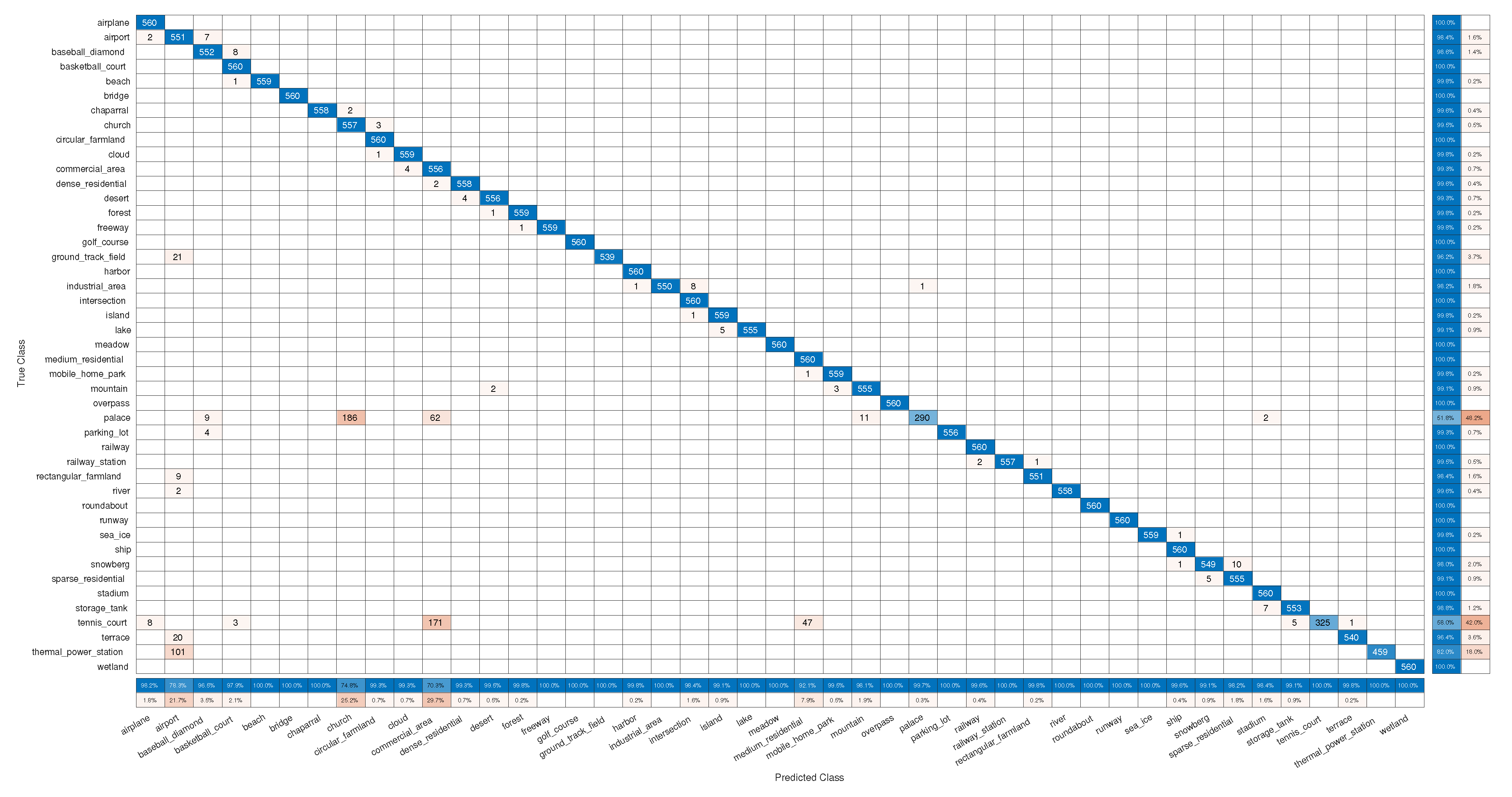
Figure 11 illustrates the confusion matrix produced by our proposed method (PBDL) with the $20\%$ training ratio. Each row represents the percentages of correctly and incorrectly classified observations for each true class. Similarly, each column displays the percentages of correctly and incorrectly classified observations for each predicted class. One can see that the classification performance of 41 categories is greater than $95\%$ where only the 14 categories achieved more than $95\%$ accuracy in the previous methods [23]. However, one common challenge is found that the church and palace are two confusing categories. This prevented many existing works to surpass such a performance [23]. In our case, $25\%$ of images from church are mistakenly classified as a palace which is $1\%$ high misclassification rate than the CNN + GCN [23]. On the other side, only $0.3\%$ of images from the palace are mistakenly classified as an industrial area where the previous methods [23] achieve $67\%$ [69] and $70\%$ accuracy performance for the palace class. By analyzing the confusion matrix on PBDL, the airport, church, and commercial area are the only challenging classes for our proposed method. Thus, the experimental results demonstrate the proposed method improves the discriminative ability of features and works well on the large-scale NWPU-RESISC45 dataset.

4.4.2. AID Dataset

We evaluate and report the comparison results against the existing state-of-the-art classification methods for the AID dataset in

Table 6. Classification accuracy (%) for the AID dataset with two training ratios.The results are obtained directly from the corresponding papers.

Method	20%	50%
Fusion by addition [32]	-	91.87 ± 0.36
D-CNN [65]	90.82 ± 0.16	96.89 ± 0.10
MDFR [67]	90.62 ± 0.27	93.37 ± 0.29
APDC-Net [68]	88.56 ± 0.29	92.15 ± 0.29
SFCNN [69]	94.93 ± 0.31	96.89 ± 0.10
Attention GANs [70]	93.97 ± 0.23	96.03 ± 0.16
CNN + GCN [23]	94.93 ± 0.31	96.89 ± 0.10
Color fusion [71]	-	94.00 ± 0.00
AlexNet+SAFF [73]	87.51 ± 0.36	91.83 ± 0.27
VGG-VD16+SAFF [73]	90.25 ± 0.29	93.83 ± 0.28
Graph CNN [72]	93.06 ± 0.26	95.78 ± 0.37
IDCCP [74]	94.80 ± 0.18	96.95 ± 0.13
SEMSDNet [75]	94.23 ± 0.63	97.64 ± 0.51
MFST [76]	96.23 ± 0.08	97.38 ± 0.08
T-CNN [77]	94.55 ± 0.27	96.72 ± 0.23
PBDL (The proposed)	96.11 ± 0.81	98.43 ± 0.33

. It could be observed that PBDL achieved the overall accuracy of $96.11\%$ and $98.43\%$ using $20\%$ and $50\%$ training ratios, respectively. As can be seen from Table 6, our method outperformed the SEMSDNet [75] with increases in the overall performance of $1.88\%$ and $0.79\%$ under both training ratios. Thus, our proposed method, by combining all the neighborhood features, verifies the effectiveness of multi-level and multi-scale feature fusion.

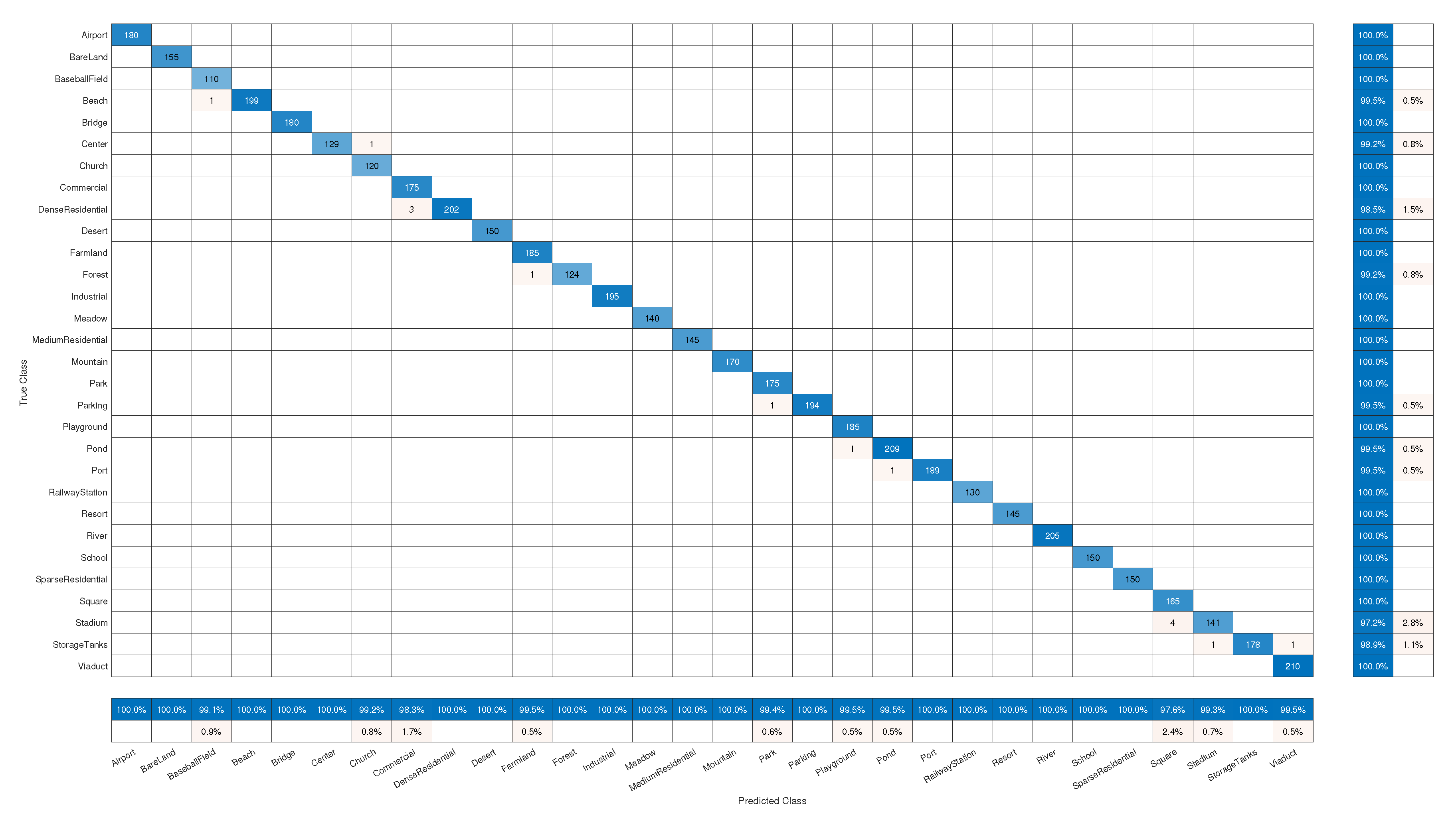
Figure 12 represents the confusion matrix generated by PBDL with the $50\%$ training ratio. As can be seen from Figure 13, the classification performance of all the categories is higher than $95\%$. Specifically, 4 of images from the square are mistakenly classified as stadium, and 3 of images from commercial are misclassified as dense residential. The five categories consisting of school, square, park, center, and resort are very confusing categories, which prevented many existing works from getting a competitive performance [75]. For instance, SFCNN [69] and the CNN + GCN [23] attained $70\%$ to $91\%$ accuracy for the class of resort while our method achieves $100\%$ accuracy. This confirms that despite the high interclass similarity, the proposed method is capable of extracting robust spatial location information to distinguish these remote sensing scene categories.

4.4.3. UC Merced Dataset

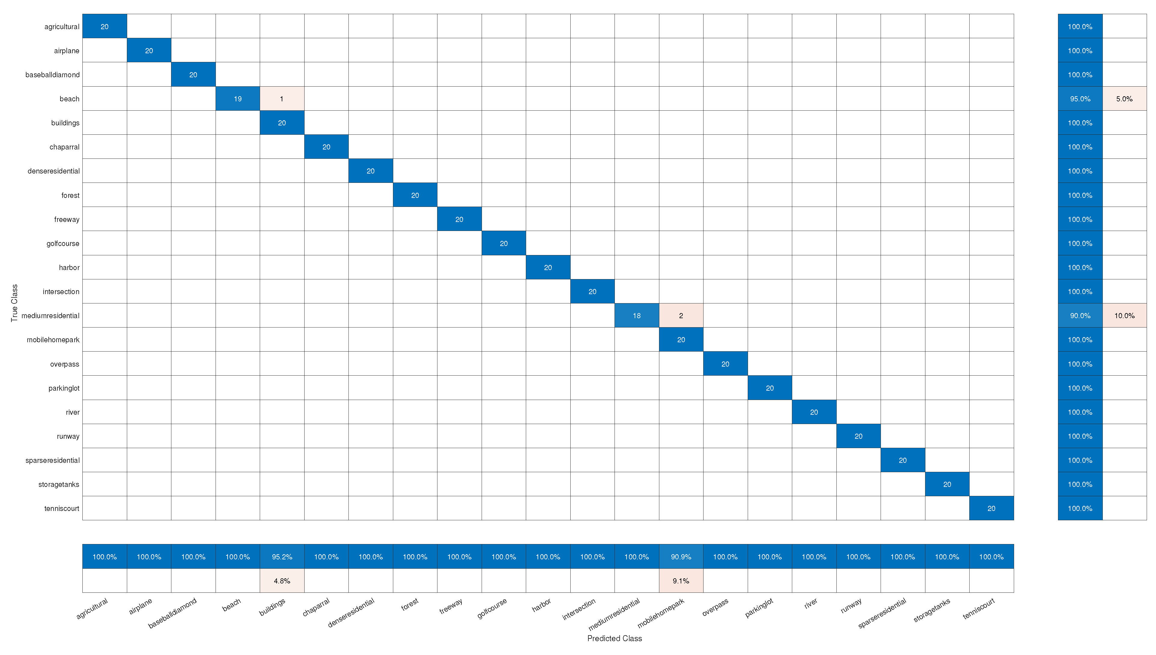
The evaluation results on the UC Merced dataset are presented in

Table 7. Comparison of classification accuracy (%) for the UC-Merced dataset with 80% ratios. The results are obtained directly from the corresponding papers.

Method	Accuracy (Mean ± std)
AlexNet+sum pooling [78]	94.10 ± 0.93
VGG-VD16+sum pooling [78]	91.67 ± 1.40
SPP-Net [79]	96.67 ± 0.94
GoogleNet [6]	94.31 ± 0.89
VGG-VD16 [6]	95.21 ± 1.20
DCA fusion [32]	96.90 ± 0.77
MCNN [80]	96.66 ± 0.90
D-CNN [65]	98.93 ± 0.10
Triple networks [66]	97.99 ± 0.53
VGG-VD16 +AlexNet [33]	98.81 ± 0.38
Fusion by concatenation [81]	98.10 ± 0.20
MDFR [67]	98.02 ± 0.51
APDC-Net [68]	97.05 ± 0.43
BoWK [34]	97.52 ± 0.80
Attention GANs [70]	97.69 ± 0.69
AlexNet+SAFF [73]	96.13 ± 0.97
VGG-VD16+SAFF [73]	97.02 ± 0.78
Color fusion [71]	98.10 ± 0.00
Graph CNN [72]	99.00 ± 0.43
IDCCP [74]	99.05 ± 0.20
SEMSDNet [75]	99.41 ± 0.14
T-CNN [77]	99.33 ± 0.11
PBDL (The proposed)	99.71 ± 0.11

. We used an $80\%$ training ratio. The proposed method achieves $99.71\%$ accuracy and competes with the previous BoW [34] approach by a margin of $2.15\%$. For further evaluation, a confusion matrix of the UC Merced dataset is shown in Figure 13. A total of 3 images are misclassified in this dataset where buildings and mobile home parks are found to be among challenging categories for our proposed method. Thus, the proposed method is effective to classify most of the scene categories.

4.4.4. WHU-RS Dataset

Table 8. Comparison of classification accuracy (%) for the WHU-RS19 with $80\%$ ratios. The results are obtained directly from the corresponding papers.

Method	Accuracy (Mean ± std)
Transferring CNNs (Case I) [82]	96.70 ± 0.00
Transferring CNNs (Case II) [82]	98.60 ± 0.00
Two-Step Categorization [83]	93.70 ± 0.57
CaffeNet [6]	94.80 ± 0.00
GoogleNet [6]	92.90 ± 0.00
VGG-VD16 [6]	95.10 ± 0.00
MDDC [84]	98.27 ± 0.53
sal$M^3$LBP-CLM [85]	96.38 ± 0.76
AlexNet-SPP-SS [79]	95.00 ± 1.12
VGG-VD19 [33]	98.16 ± 0.77
DCA by addition [32]	98.70 ± 0.22
MLF [86]	88.16 ± 2.76
Fusion by concatenation [81]	99.17 ± 0.20
D-DSML-CaffeNet [87]	96.64 ± 0.68
BoWK [34]	99.47 ± 0.60
Color fusion [71]	96.60 ± 0.00
PBDL (The proposed)	99.63 ± 0.42

reports the comparison results of the WHU-RS dataset. As shown in Table 8, the PBDL achieves the highest classification $(99.63\%)$ accuracy and outperforms all the previous methods. In addition, a confusion matrix of the WHU-RS dataset is shown in Figure 6d. Tremendous improvements can be observed in some classes such as residential, industrial, port, pond, park, mountain, airport, and railway station. Only 2 images from commercial and bridge categories are misclassified in this dataset. Hence, based on experimental analysis, we argue that a combination of neighborhood sizes and multi-scale filtering is essential to produce a robust feature representation for remote sensing scene classification.

5. Conclusions

This paper introduced a simple, yet very effective approach called patch-based discriminative learning (PBDL) for extracting discriminative patch features. The PBCL generates N patches for each image feature map, and the individual patches of the same image are located at different spatial regions to achieve a more accurate representation. In particular, these regions focus on “where” is the discriminative information, whereas aggregation (fusion) of the neighborhood regions focuses on “what” is the scene semantic associated with, given an input image and taking into account the complementary aspect. We showed that patch-based learning in the BoW model significantly improves the recognition performance compared to that obtained when using a single-level BoW alone. Experiments were conducted on four publicly available datasets, and the results reinforced the intuition that the use of different distributions of spatial location and visual information is crucial for scene classification. The proposed approach is shown to have advantages over single-scale BoW and traditional CNNs methods, especially in the situation where a large number of training data is not available and the classification accuracy is the prime goal. A drawback of PBDL is that it increases the computational complexity of the BoW model. Therefore, we plan to extend our work by developing computationally efficient methods to automatically obtain multi-level and multi-scale features without human intervention.

References

1. Rujoiu-Mare, M.R.; Mihai, B.A. Mapping land cover using remote sensing data and GIS techniques: A case study of Prahova Subcarpathians. Procedia Environ. Sci. 2016, 32, 244–255. [Google Scholar] [CrossRef] [Green Version]
2. Li, Y.; Ma, J.; Zhang, Y. Image retrieval from remote sensing big data: A survey. Inf. Fusion 2021, 67, 94–115. [Google Scholar] [CrossRef]
3. Joyce, K.E.; Belliss, S.E.; Samsonov, S.V.; McNeill, S.J.; Glassey, P.J. A review of the status of satellite remote sensing and image processing techniques for mapping natural hazards and disasters. Prog. Phys. Geogr. 2009, 33, 183–207. [Google Scholar] [CrossRef] [Green Version]
4. Treitz, P.; Rogan, J. Remote sensing for mapping and monitoring land-cover and land-use change-an introduction. Prog. Plan. 2004, 61, 269–279. [Google Scholar] [CrossRef]
5. Bishop-Taylor, R.; Nanson, R.; Sagar, S.; Lymburner, L. Mapping Australia’s dynamic coastline at mean sea level using three decades of Landsat imagery. Remote Sens. Environ. 2021, 267, 112734. [Google Scholar] [CrossRef]
6. Xia, G.S.; Hu, J.; Hu, F.; Shi, B.; Bai, X.; Zhong, Y.; Zhang, L.; Lu, X. AID: A benchmark data set for performance evaluation of aerial scene classification. IEEE Trans. Geosci. Remote Sens. 2017, 55, 3965–3981. [Google Scholar] [CrossRef] [Green Version]
7. Cheng, G.; Xie, X.; Han, J.; Guo, L.; Xia, G.S. Remote sensing image scene classification meets deep learning: Challenges, methods, benchmarks, and opportunities. IEEE J. Sel. Top. Appl. Earth Obs. Remote Sens. 2020, 13, 3735–3756. [Google Scholar] [CrossRef]
8. He, D.C.; Wang, L. Texture unit, texture spectrum, and texture analysis. IEEE Trans. Geosci. Remote Sens. 1990, 28, 509–512. [Google Scholar]
9. Lowe, D.G. Distinctive image features from scale-invariant keypoints. Int. J. Comput. Vis. 2004, 60, 91–110. [Google Scholar] [CrossRef]
10. Swain, M.; Ballard, D. Color Indexing. Int. J. Comput. Vis. 1991, 7, 11–23. [Google Scholar] [CrossRef]
11. Dalal, N.; Triggs, B. Histograms of oriented gradients for human detection. In Proceedings of the 2005 IEEE Computer Society Conference on Computer Vision and Pattern Recognition (CVPR’05), San Diego, CA, USA, 20–25 June 2005; Volume 1, pp. 886–893. [Google Scholar]
12. Tsai, C.F. Bag-of-words representation in image annotation: A review. Int. Sch. Res. Not. 2012, 2012, 376804. [Google Scholar] [CrossRef]
13. Li, X.; Zhang, L.; Wang, L.; Wan, X. Effects of BOW model with affinity propagation and spatial pyramid matching on polarimetric SAR image classification. IEEE J. Sel. Top. Appl. Earth Obs. Remote Sens. 2017, 10, 3314–3322. [Google Scholar] [CrossRef]
14. Lazebnik, S.; Schmid, C.; Ponce, J. Beyond bags of features: Spatial pyramid matching for recognizing natural scene categories. In Proceedings of the 2006 IEEE Computer Society Conference on Computer Vision and Pattern Recognition (CVPR’06), New York, NY, USA, 17–22 June 2006; Volume 2, pp. 2169–2178. [Google Scholar]
15. Shi, C.; Zhang, X.; Sun, J.; Wang, L. Remote Sensing Scene Image Classification Based on Dense Fusion of Multi-level Features. Remote Sens. 2021, 13, 4379. [Google Scholar] [CrossRef]
16. Yuan, B.; Han, L.; Gu, X.; Yan, H. Multi-deep features fusion for high-resolution remote sensing image scene classification. Neural Comput. Appl. 2021, 33, 2047–2063. [Google Scholar] [CrossRef]
17. Gao, H.; Chen, Z.; Xu, F. Adaptive spectral-spatial feature fusion network for hyperspectral image classification using limited training samples. Int. J. Appl. Earth Obs. Geoinf. 2022, 107, 102687. [Google Scholar] [CrossRef]
18. Jiang, H.; Peng, M.; Zhong, Y.; Xie, H.; Hao, Z.; Lin, J.; Ma, X.; Hu, X. A Survey on Deep Learning-Based Change Detection from High-Resolution Remote Sensing Images. Remote Sens. 2022, 14, 1552. [Google Scholar] [CrossRef]
19. Springenberg, J.T.; Dosovitskiy, A.; Brox, T.; Riedmiller, M. Striving for simplicity: The all convolutional net. arXiv 2014, arXiv:1412.6806. [Google Scholar]
20. Hu, J.; Xia, G.S.; Hu, F.; Sun, H.; Zhang, L. A comparative study of sampling analysis in scene classification of high-resolution remote sensing imagery. In Proceedings of the 2015 IEEE International Geoscience and Remote Sensing Symposium (IGARSS), Milan, Italy, 26–31 July 2015; pp. 2389–2392. [Google Scholar]
21. Muhammad, U.; Wang, W.; Chattha, S.P.; Ali, S. Pre-trained VGGNet architecture for remote-sensing image scene classification. In Proceedings of the 2018 24th International Conference on Pattern Recognition (ICPR), Beijing, China, 20–24 August 2018; pp. 1622–1627. [Google Scholar]
22. Bi, Q.; Qin, K.; Li, Z.; Zhang, H.; Xu, K.; Xia, G.S. A multiple-instance densely-connected ConvNet for aerial scene classification. IEEE Trans. Image Process. 2020, 29, 4911–4926. [Google Scholar] [CrossRef]
23. Liang, J.; Deng, Y.; Zeng, D. A deep neural network combined CNN and GCN for remote sensing scene classification. IEEE J. Sel. Top. Appl. Earth Obs. Remote Sens. 2020, 13, 4325–4338. [Google Scholar] [CrossRef]
24. Ghaffarian, S.; Valente, J.; Van Der Voort, M.; Tekinerdogan, B. Effect of attention mechanism in deep-learning-based remote sensing image processing: A systematic literature review. Remote Sens. 2021, 13, 2965. [Google Scholar] [CrossRef]
25. Jurie, F.; Triggs, B. Creating efficient codebooks for visual recognition. In Proceedings of the Tenth IEEE International Conference on Computer Vision (ICCV’05), Beijing, China, 17–21 October 2005; Volume 1, pp. 604–610. [Google Scholar]
26. Nowak, E.; Jurie, F.; Triggs, B. Sampling strategies for bag-of-features image classification. In Proceedings of the European Conference on Computer Vision; Springer: Berlin/Heidelberg, Germany, 2006; pp. 490–503. [Google Scholar]
27. Agarwal, S.; Awan, A.; Roth, D. Learning to detect objects in images via a sparse, part-based representation. IEEE Trans. Pattern Anal. Mach. Intell. 2004, 26, 1475–1490. [Google Scholar] [CrossRef]
28. Tuytelaars, T. Dense interest points. In Proceedings of the 2010 IEEE Computer Society Conference on Computer Vision and Pattern Recognition, San Francisco, CA, USA, 13–18 June 2010; pp. 2281–2288. [Google Scholar]
29. Chen, Z.; Zhu, Y.; Zhao, C.; Hu, G.; Zeng, W.; Wang, J.; Tang, M. Dpt: Deformable patch-based transformer for visual recognition. In Proceedings of the 29th ACM International Conference on Multimedia, 20–24 October 2021; pp. 2899–2907. [Google Scholar]
30. Lindeberg, T. Scale-Space Theory Computer Vision; Springer Science & Business Media: Berlin/Heidelberg, Germany, 2013; Volume 256. [Google Scholar]
31. Bay, H.; Ess, A.; Tuytelaars, T.; Van Gool, L. Speeded-up robust features (SURF). Comput. Vis. Image Underst. 2008, 110, 346–359. [Google Scholar] [CrossRef]
32. Chaib, S.; Liu, H.; Gu, Y.; Yao, H. Deep feature fusion for VHR remote sensing scene classification. IEEE Trans. Geosci. Remote Sens. 2017, 55, 4775–4784. [Google Scholar] [CrossRef]
33. Li, E.; Xia, J.; Du, P.; Lin, C.; Samat, A. Integrating multilayer features of convolutional neural networks for remote sensing scene classification. IEEE Trans. Geosci. Remote Sens. 2017, 55, 5653–5665. [Google Scholar] [CrossRef]
34. Muhammad, U.; Wang, W.; Hadid, A.; Pervez, S. Bag of words KAZE (BoWK) with two-step classification for high-resolution remote sensing images. IET Comput. Vis. 2019, 13, 395–403. [Google Scholar] [CrossRef]
35. Schuster, M.; Paliwal, K.K. Bidirectional recurrent neural networks. IEEE Trans. Signal Process. 1997, 45, 2673–2681. [Google Scholar] [CrossRef] [Green Version]
36. Blaschke, T.; Strobl, J. What’s wrong with pixels? Some recent developments interfacing remote sensing and GIS. Z. Geoinf. 2001, 12–17. [Google Scholar]
37. Chen, L.; Yang, W.; Xu, K.; Xu, T. Evaluation of local features for scene classification using VHR satellite images. In Proceedings of the 2011 Joint Urban Remote Sensing Event, Munich, Germany, 11–13 April 2011; pp. 385–388. [Google Scholar]
38. Tokarczyk, P.; Wegner, J.D.; Walk, S.; Schindler, K. Features, color spaces, and boosting: New insights on semantic classification of remote sensing images. IEEE Trans. Geosci. Remote Sens. 2014, 53, 280–295. [Google Scholar] [CrossRef]
39. Yu, H.; Yang, W.; Xia, G.S.; Liu, G. A color-texture-structure descriptor for high-resolution satellite image classification. Remote Sens. 2016, 8, 259. [Google Scholar] [CrossRef] [Green Version]
40. Zhang, F.; Yang, X. Improving land cover classification in an urbanized coastal area by random forests: The role of variable selection. Remote Sens. Environ. 2020, 251, 112105. [Google Scholar] [CrossRef]
41. Yang, Y.; Newsam, S. Geographic image retrieval using local invariant features. IEEE Trans. Geosci. Remote Sens. 2012, 51, 818–832. [Google Scholar] [CrossRef]
42. Khan, F.S.; Van de Weijer, J.; Vanrell, M. Modulating shape features by color attention for object recognition. Int. J. Comput. Vis. 2012, 98, 49–64. [Google Scholar] [CrossRef]
43. Yang, Y.; Newsam, S. Bag-of-visual-words and spatial extensions for land-use classification. In Proceedings of the 18th SIGSPATIAL International Conference on Advances in Geographic Information Systems, San Jose, CA, USA, 2–5 November 2010; pp. 270–279. [Google Scholar]
44. Vigo, D.A.R.; Khan, F.S.; Van De Weijer, J.; Gevers, T. The impact of color on bag-of-words based object recognition. In Proceedings of the 2010 20th International Conference on Pattern Recognition, Istanbul, Turkey, 23–26 August 2010; pp. 1549–1553. [Google Scholar]
45. Van De Sande, K.; Gevers, T.; Snoek, C. Evaluating color descriptors for object and scene recognition. IEEE Trans. Pattern Anal. Mach. Intell. 2009, 32, 1582–1596. [Google Scholar] [CrossRef] [PubMed]
46. Yang, J.; Yu, K.; Gong, Y.; Huang, T. Linear spatial pyramid matching using sparse coding for image classification. In Proceedings of the 2009 IEEE Conference on Computer Vision and Pattern Recognition, Miami, FL, USA, 20–25 June 2009; pp. 1794–1801. [Google Scholar]
47. Ghanbari, H.; Mahdianpari, M.; Homayouni, S.; Mohammadimanesh, F. A meta-analysis of convolutional neural networks for remote sensing applications. IEEE J. Sel. Top. Appl. Earth Obs. Remote Sens. 2021, 14, 3602–3613. [Google Scholar] [CrossRef]
48. Zuo, Z.; Shuai, B.; Wang, G.; Liu, X.; Wang, X.; Wang, B.; Chen, Y. Convolutional recurrent neural networks: Learning spatial dependencies for image representation. In Proceedings of the IEEE Conference on Computer Vision and Pattern Recognition Workshops, Boston, MA, USA, 7–12 June 2015; pp. 18–26. [Google Scholar]
49. Huang, R.; Zheng, F.; Huang, W. Multi-label Remote Sensing Image Annotation with Multi-scale attention and Label Correlation. IEEE J. Sel. Top. Appl. Earth Obs. Remote Sens. 2021, 14, 6951–6961. [Google Scholar] [CrossRef]
50. Li, M.; Lei, L.; Li, X.; Sun, Y.; Kuang, G. An adaptive multilayer feature fusion strategy for remote sensing scene classification. Remote Sens. Lett. 2021, 12, 563–572. [Google Scholar] [CrossRef]
51. Li, L.; Han, J.; Yao, X.; Cheng, G.; Guo, L. DLA-MatchNet for few-shot remote sensing image scene classification. IEEE Trans. Geosci. Remote Sens. 2020, 59, 7844–7853. [Google Scholar] [CrossRef]
52. Yao, X.; Han, J.; Cheng, G.; Qian, X.; Guo, L. Semantic annotation of high-resolution satellite images via weakly supervised learning. IEEE Trans. Geosci. Remote Sens. 2016, 54, 3660–3671. [Google Scholar] [CrossRef]
53. Rosier, J.F.; Taubenböck, H.; Verburg, P.H.; van Vliet, J. Fusing Earth observation and socioeconomic data to increase the transferability of large-scale urban land use classification. Remote Sens. Environ. 2022, 278, 113076. [Google Scholar] [CrossRef]
54. Bahdanau, D.; Cho, K.; Bengio, Y. Neural machine translation by jointly learning to align and translate. arXiv 2014, arXiv:1409.0473. [Google Scholar]
55. Chen, S.; Liu, H.; Zeng, X.; Qian, S.; Wei, W.; Wu, G.; Duan, B. Local patch vectors encoded by fisher vectors for image classification. Information 2018, 9, 38. [Google Scholar] [CrossRef] [Green Version]
56. Chavez, A.J. Image Classification with Dense SIFT Sampling: An Exploration of Optimal Parameters; Kansas State University: Manhattan, KS, USA, 2012. [Google Scholar]
57. Witkin, A. Scale-space filtering: A new approach to multi-scale description. In Proceedings of the ICASSP’84. IEEE International Conference on Acoustics, Speech, and Signal Processing, San Diego, CA, USA, 19–21 March 1984; Volume 9, pp. 150–153. [Google Scholar]
58. Lee, J.H. Panoramic image stitching using feature extracting and matching on embedded system. Trans. Electr. Electron. Mater. 2017, 18, 273–278. [Google Scholar]
59. Sun, Q.S.; Zeng, S.G.; Liu, Y.; Heng, P.A.; Xia, D.S. A new method of feature fusion and its application in image recognition. Pattern Recognit. 2005, 38, 2437–2448. [Google Scholar] [CrossRef]
60. Sheng, G.; Yang, W.; Xu, T.; Sun, H. High-resolution satellite scene classification using a sparse coding based multiple feature combination. Int. J. Remote Sens. 2012, 33, 2395–2412. [Google Scholar] [CrossRef]
61. Cheng, G.; Han, J.; Lu, X. Remote sensing image scene classification: Benchmark and state of the art. Proc. IEEE 2017, 105, 1865–1883. [Google Scholar] [CrossRef]
62. Glorot, X.; Bengio, Y. Understanding the difficulty of training deep feedforward neural networks. In Proceedings of the Thirteenth International Conference on Artificial Intelligence and Statistics, JMLR Workshop and Conference Proceedings, Chia Laguna Resort, Italy, 13–15 May 2010; pp. 249–256. [Google Scholar]
63. Van der Maaten, L.; Hinton, G. Visualizing data using t-SNE. J. Mach. Learn. Res. 2008, 9, 2579–2605. [Google Scholar]
64. Cheng, G.; Li, Z.; Yao, X.; Guo, L.; Wei, Z. Remote sensing image scene classification using bag of convolutional features. IEEE Geosci. Remote Sens. Lett. 2017, 14, 1735–1739. [Google Scholar] [CrossRef]
65. Cheng, G.; Yang, C.; Yao, X.; Guo, L.; Han, J. When deep learning meets metric learning: Remote sensing image scene classification via learning discriminative CNNs. IEEE Trans. Geosci. Remote Sens. 2018, 56, 2811–2821. [Google Scholar] [CrossRef]
66. Liu, Y.; Huang, C. Scene classification via triplet networks. IEEE J. Sel. Top. Appl. Earth Obs. Remote Sens. 2017, 11, 220–237. [Google Scholar] [CrossRef]
67. Zhang, J.; Zhang, M.; Shi, L.; Yan, W.; Pan, B. A multi-scale approach for remote sensing scene classification based on feature maps selection and region representation. Remote Sens. 2019, 11, 2504. [Google Scholar] [CrossRef] [Green Version]
68. Bi, Q.; Qin, K.; Zhang, H.; Xie, J.; Li, Z.; Xu, K. APDC-Net: Attention pooling-based convolutional network for aerial scene classification. IEEE Geosci. Remote Sens. Lett. 2019, 17, 1603–1607. [Google Scholar] [CrossRef]
69. Xie, J.; He, N.; Fang, L.; Plaza, A. Scale-free convolutional neural network for remote sensing scene classification. IEEE Trans. Geosci. Remote Sens. 2019, 57, 6916–6928. [Google Scholar] [CrossRef]
70. Yu, Y.; Li, X.; Liu, F. Attention GANs: Unsupervised deep feature learning for aerial scene classification. IEEE Trans. Geosci. Remote Sens. 2019, 58, 519–531. [Google Scholar] [CrossRef]
71. Anwer, R.M.; Khan, F.S.; Laaksonen, J. Compact Deep Color Features for Remote Sensing Scene Classification. Neural Process. Lett. 2021, 53, 1523–1544. [Google Scholar] [CrossRef]
72. Gao, Y.; Shi, J.; Li, J.; Wang, R. Remote sensing scene classification based on high-order graph convolutional network. Eur. J. Remote Sens. 2021, 54, 141–155. [Google Scholar] [CrossRef]
73. Cao, R.; Fang, L.; Lu, T.; He, N. Self-attention-based deep feature fusion for remote sensing scene classification. IEEE Geosci. Remote Sens. Lett. 2020, 18, 43–47. [Google Scholar] [CrossRef]
74. Wang, S.; Ren, Y.; Parr, G.; Guan, Y.; Shao, L. Invariant Deep Compressible Covariance Pooling for Aerial Scene Categorization. IEEE Trans. Geosci. Remote Sens. 2020, 59, 6549–6561. [Google Scholar] [CrossRef]
75. Tian, T.; Li, L.; Chen, W.; Zhou, H. SEMSDNet: A Multi-Scale Dense Network with Attention for Remote Sensing Scene Classification. IEEE J. Sel. Top. Appl. Earth Obs. Remote Sens. 2021, 14, 5501–5514. [Google Scholar] [CrossRef]
76. Wang, G.; Zhang, N.; Liu, W.; Chen, H.; Xie, Y. MFST: A Multi-Level Fusion Network for Remote Sensing Scene Classification. IEEE Geosci. Remote Sens. Lett. 2022, 19, 1–5. [Google Scholar] [CrossRef]
77. Wang, W.; Chen, Y.; Ghamisi, P. Transferring CNN With Adaptive Learning for Remote Sensing Scene Classification. IEEE Trans. Geosci. Remote Sens. 2022, 60, 1–18. [Google Scholar] [CrossRef]
78. Babenko, A.; Lempitsky, V. Aggregating local deep features for image retrieval. In Proceedings of the IEEE International Conference on Computer Vision, Santiago, Chile, 7–13 December 2015; pp. 1269–1277. [Google Scholar]
79. Han, X.; Zhong, Y.; Cao, L.; Zhang, L. Pre-trained alexnet architecture with pyramid pooling and supervision for high spatial resolution remote sensing image scene classification. Remote Sens. 2017, 9, 848. [Google Scholar] [CrossRef] [Green Version]
80. Liu, Y.; Zhong, Y.; Qin, Q. Scene classification based on multiscale convolutional neural network. IEEE Trans. Geosci. Remote Sens. 2018, 56, 7109–7121. [Google Scholar] [CrossRef] [Green Version]
81. Muhammad, U.; Wang, W.; Hadid, A. Feature fusion with deep supervision for remote-sensing image scene classification. In Proceedings of the 2018 IEEE 30th International Conference on Tools with Artificial Intelligence (ICTAI), Volos, Greece, 5–7 November 2018; pp. 249–253. [Google Scholar]
82. Hu, F.; Xia, G.S.; Hu, J.; Zhang, L. Transferring deep convolutional neural networks for the scene classification of high-resolution remote sensing imagery. Remote Sens. 2015, 7, 14680–14707. [Google Scholar] [CrossRef] [Green Version]
83. Yan, L.; Zhu, R.; Mo, N.; Liu, Y. Improved class-specific codebook with two-step classification for scene-level classification of high resolution remote sensing images. Remote Sens. 2017, 9, 223. [Google Scholar] [CrossRef] [Green Version]
84. Qi, K.; Yang, C.; Guan, Q.; Wu, H.; Gong, J. A multiscale deeply described correlatons-based model for land-use scene classification. Remote Sens. 2017, 9, 917. [Google Scholar] [CrossRef] [Green Version]
85. Bian, X.; Chen, C.; Tian, L.; Du, Q. Fusing local and global features for high-resolution scene classification. IEEE J. Sel. Top. Appl. Earth Obs. Remote Sens. 2017, 10, 2889–2901. [Google Scholar] [CrossRef]
86. Li, E.; Du, P.; Samat, A.; Meng, Y.; Che, M. Mid-level feature representation via sparse autoencoder for remotely sensed scene classification. IEEE J. Sel. Top. Appl. Earth Obs. Remote Sens. 2016, 10, 1068–1081. [Google Scholar] [CrossRef]
87. Gong, Z.; Zhong, P.; Yu, Y.; Hu, W. Diversity-promoting deep structural metric learning for remote sensing scene classification. IEEE Trans. Geosci. Remote Sens. 2017, 56, 371–390. [Google Scholar] [CrossRef]
Figure 1. The challenging scene images of AID dataset [6]. (a) The intra-class diversity and (b) inter-class similarity are the main obstacles that limit the scene classification performance.
Remotesensing 14 05913 g001
Figure 2. An illustration of different patch sizes. Given a remote sensing image, the BoW model is designed with different image patch sizes to incorporate spatial information. Left column: Example images from NWPU dataset. Right columns: SURF [31] features of light, medium and dark green colors represent different spatial locations.
Remotesensing 14 05913 g002
Figure 3. Flowchart of the proposed method. The local patches are selected by a fixed-size sliding window, where green, orange, blue, and yellow rectangles represent the patch sizes of 10 × 10 , 8 × 8 , 6 × 6 , and 4 × 4 , respectively. Then the dense interest points are extracted with Gaussian second derivatives without changing the size of the original image and encoded to visual vocabulary through the k-means clustering process. Finally, a concatenated histogram is used as an input for training the BiLSTM network.
Remotesensing 14 05913 g003
Figure 4. Predefined patch ( 4 × 4 ) size before representing features over entire image.
Remotesensing 14 05913 g004
Figure 5. Scene recognition with dense sampling, sparse interest points and the proposed dense interest points.
Remotesensing 14 05913 g005
Figure 6. Confusion matrix of our proposed method on WHU-RS dataset by fixing the training ratio as 80 % training (a) with one-stage learning, (b) with two-stage learning, (c) with three-stage learning, and (d) with multi-stage learning. Zoom in for a better view.
Remotesensing 14 05913 g006aRemotesensing 14 05913 g006b
Figure 7. Classification accuracy of the proposed method under different Gaussian scales for four datasets.
Remotesensing 14 05913 g007
Figure 8. Comparing the performance on WHU-RS dataset with SURF-BOW [31], SPM-BOW [14], and ours.
Remotesensing 14 05913 g008
Figure 9. Images indicate window size and stride for each one of the three. (Leftright): sample windows shows high redundancy. Center: sample windows with a pixel width 2 display overlapping. Right: the proposed sample windows show negligible redundancy.
Remotesensing 14 05913 g009
Figure 10. Two-dimensional scatterplots of SURF-based BoW features generated with t-SNE over the WHU-RS dataset. (a) Scatterplot of one-stage multi-scale features. (b) Scatterplot of features extracted and combined from four-stage learning. (c) Features extracted from the last fully-connected layer of BiLSTM. All points in the scatterplots are color coded by class. Zoom in for a better view.
Remotesensing 14 05913 g010
Figure 11. Confusion matrix of our proposed method on NWPU-RESISC45 Dataset by fixing the training ratio as 20 % . Zoom in for a better view.
Remotesensing 14 05913 g011
Figure 12. Confusion matrix of our proposed method on AID Dataset by fixing the training ratio as 50 % . Zoom in for a better view.
Remotesensing 14 05913 g012
Figure 13. Confusion matrix of our proposed method on UC Merced Dataset by fixing the training ratio as 80 % . Zoom in for a better view.
Remotesensing 14 05913 g013