MFNet: Multi-Level Feature Extraction and Fusion Network for Large-Scale Point Cloud Classification

Abstract

The accuracy with which a neural network interprets a point cloud depends on the quality of the features expressed by the network. Addressing this issue, we propose a multi-level feature extraction layer (MFEL) which collects local contextual feature and global information by modeling point clouds at different levels. The MFEL is mainly composed of three independent modules, including the aggregated GAPLayer, the spatial position perceptron, and the RBFLayer, which learn point cloud features from three different scales. The aggregated GAPLayer aggregates the geometry features of neighboring points in a local coordinate system to centroid by graph convolution. Then, the spatial position perceptron independently learns the position features of each point in the world coordinate system. Finally, the RBFLayer aggregates points into pointsets according to the correlation between features, and extracts features from the pointset scale through the quantization layer. Based on the MFEL, an end-to-end classification and segmentation network, namely the MFNet and MFNet-S, is proposed. In the proposed network, the channel-attention mechanism is employed to better aggregate multi-level features. We conduct classification and semantic segmentation experiments on four standard datasets. The results show that the proposed method outperforms the compared methods on the multiple datasets, resulting in 93.1% classification accuracy in ModelNet40. Furthermore, the mIoU of part semantic segmentation in ShapeNet is 85.4%, and the mIoU for semantic segmentation in S3DIS and Semantic3D is 62.9% and 71.9%, respectively.

1. Introduction

Point clouds contain rich three-dimensional (3D) spatial information and have broad application prospects in areas such as autonomous driving, virtual reality, and power grid inspection [1,2]. However, the automatic extraction of interesting information from point clouds, especially in large-scale scenes, remains a huge challenge [3]. This is because objects in a large scene usually exit a lot of occlusions. Moreover, objects of different classes but with a similar local geometry structure will cause interference for segmentation. Therefore, it is necessary to describe the objects in the large-scale scene from different scales to achieve the effect of efficient extraction [4].

Deep learning methods based on convolutional neural networks (CNNs) have achieved great success in the field of two-dimensional (2D) image processing. However, directly migrating these image processing networks to 3D point cloud processing tasks is usually infeasible because point clouds are disordered and structurally irregular. Moreover, point clouds contain a large amount of object geometry information, which does not exist in 2D images. In addition, the point cloud collected in the real scene has a large coverage and uneven density of point, but the resolution of the image is fixed. Therefore, how to utilize the geometric features and multi-granularity features of point clouds are two challenges in the field of point cloud interpretation [5].

The disorder of the point cloud is the problem to be considered primarily in point cloud processing networks based on deep learning. The disordered point clouds can be transformed into a regular form by some strategies, e.g., voxelization [6] and multi-view projection [7,8]. Another idea is to design a symmetric function (such as max-pooling) to counteract the disorder of point clouds. The representative work is PointNet [9] and its successor, PointNet++ [10]. PointNet learns the point-wise features using a shared multi-layer perception (MLP) but fails to capture local geometry patterns among neighboring points. PointNet++ tries to learn local contexts by aggregating per-point features in a neighborhood. However, it still deals with each point separately within each neighborhood, and the geometric relations between points are not fully utilized.

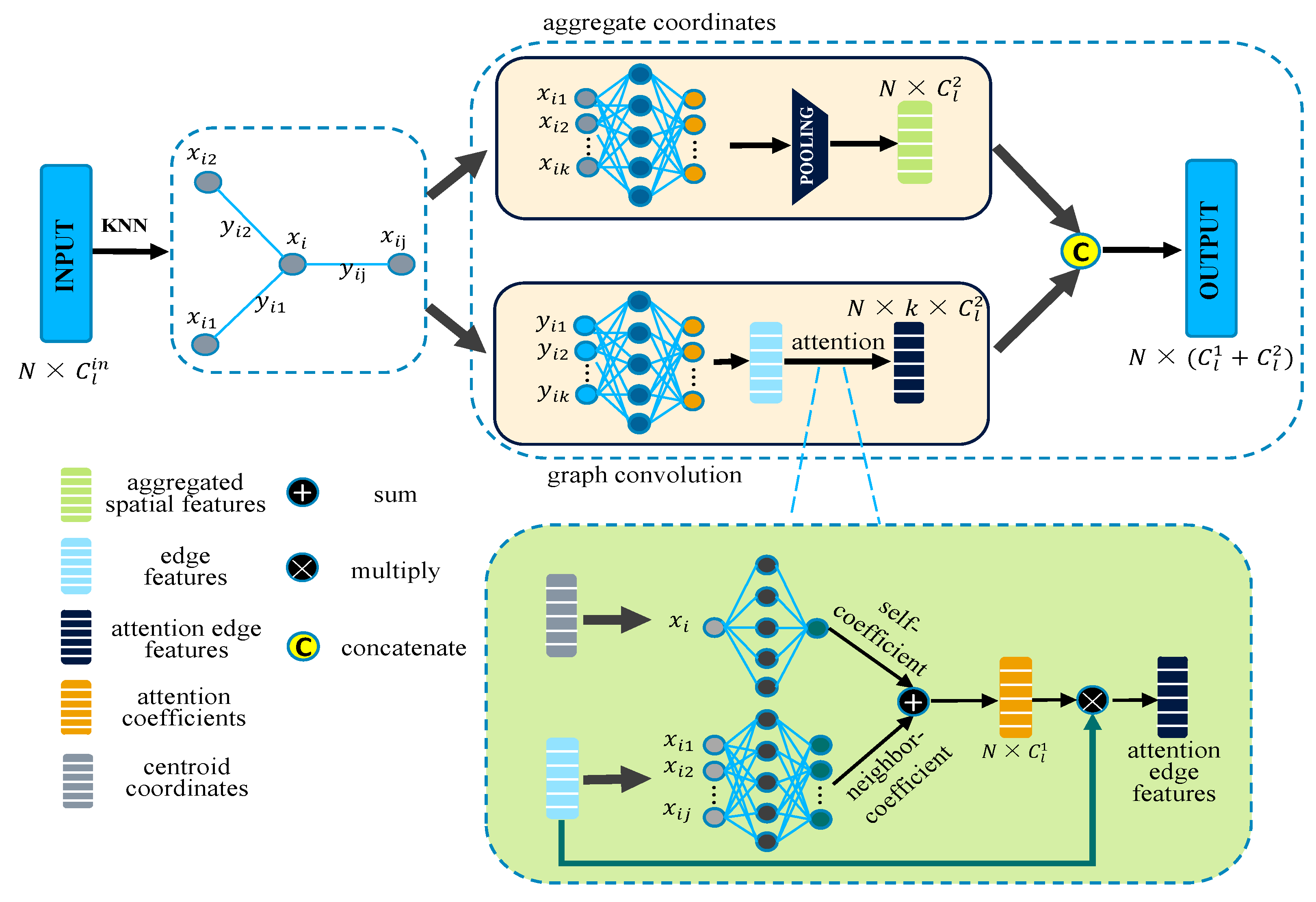
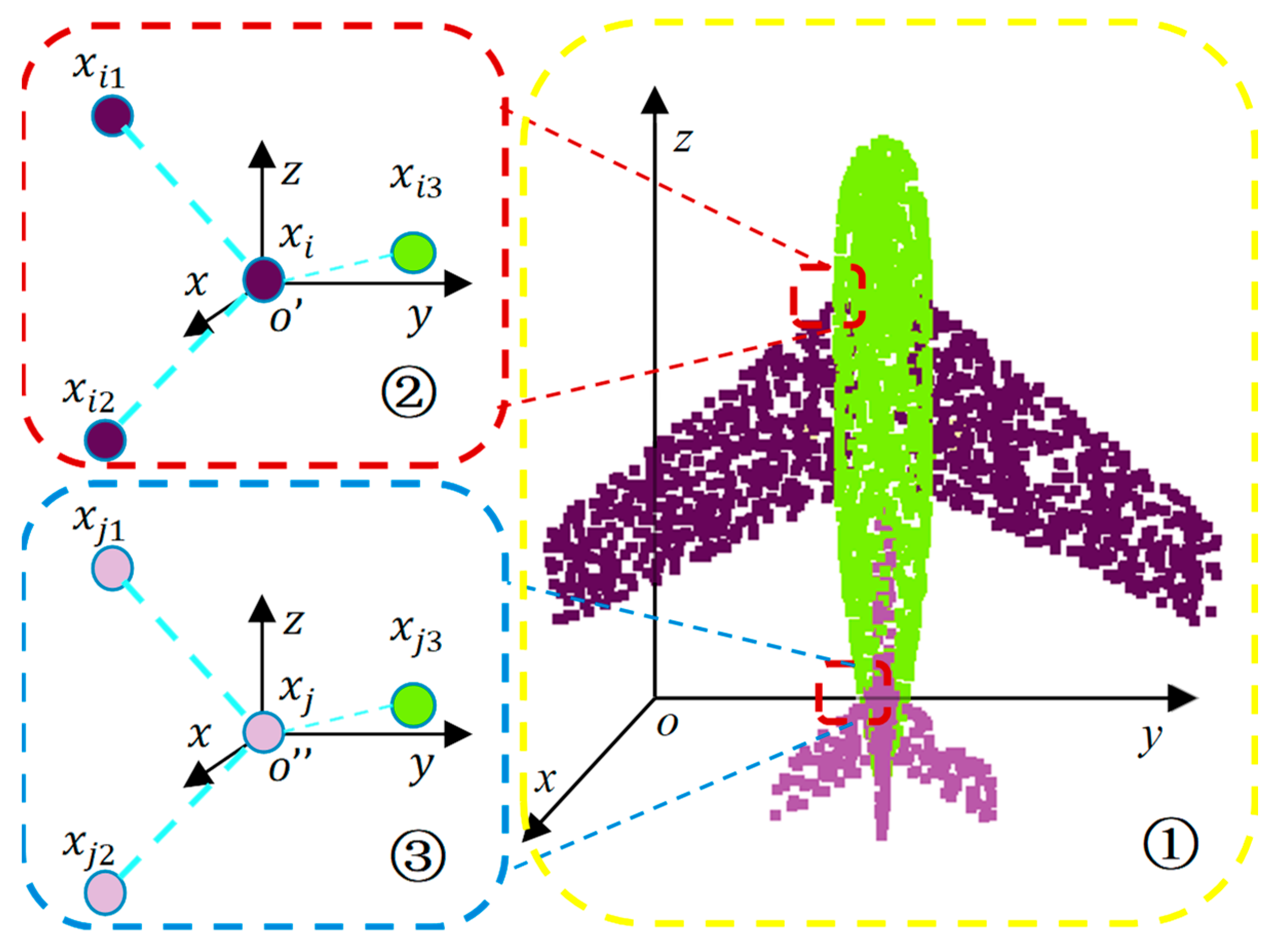
In order to obtain more geometric structure information from local neighborhoods, some researchers have proposed some neighborhood-based feature extraction methods. For instance, A-CNN [11] and KPConv [12] define convolution kernels within the neighborhood to extract features such as the spatial location of each neighborhood point, and then aggregate the features to the center point. GAPNet [13] proposes the GAPLayer (namely a multi-head graph attention-based point network layer) which convolves edges to extract the geometric features of a graph. Then, it generates local attention weights and self-attention weights according to local features and assigns attention weights to each edge. The GAPNet has made great contributions to graph attention, but it mainly focuses on point-to-point relationships within neighborhoods and performs poorly on large-scale datasets. We boil it down to three reasons.

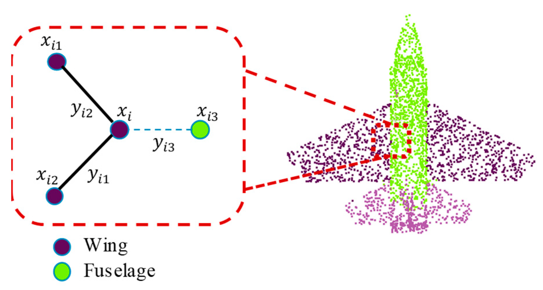
Firstly, as shown in Figure 1, some point clouds may have similar geometries, but they may belong to different categories, as shown by the rectangles ② and ③. As mentioned above, the GAPLayer can only identify the geometric features of a local region but cannot effectively correlate them with the wider contextual information of the region. Therefore, the situation shown in Figure 1 may be a hindrance when interpreting point clouds.

Secondly, the GAPLayer processes each local region independently, regardless of the correlation between regions, as shown in Figure 2.

Finally, global features play an important role in classification and part segmentation. Although the GAPLayer does mention global feature extraction, it does not blend well with features at other scales.

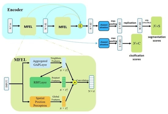
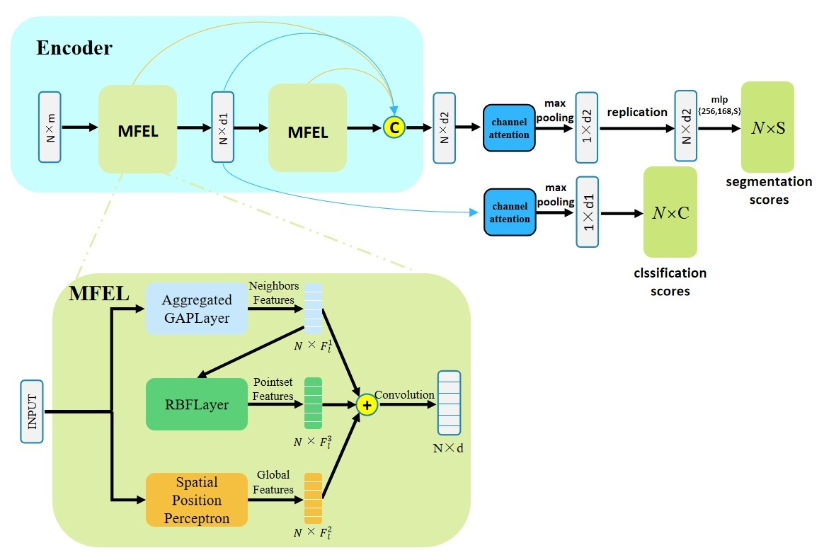
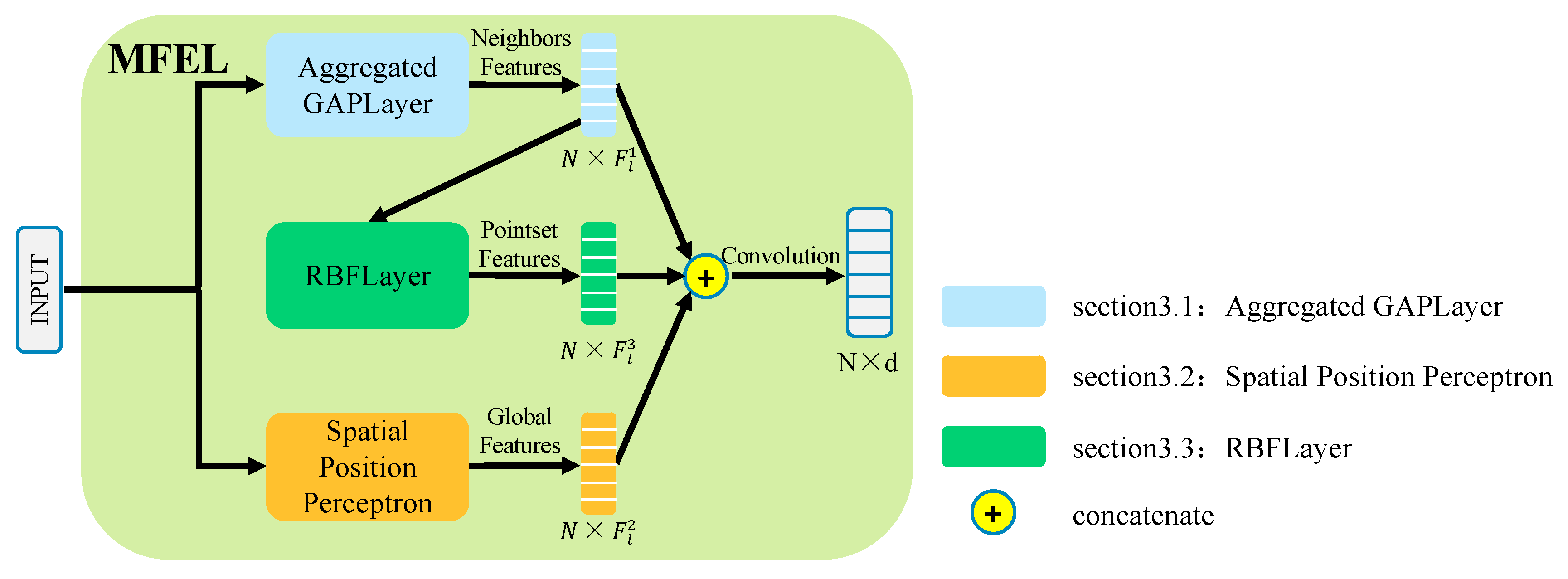
In order to address the above problems and avoid the loss of information caused by down-sampling, we propose the MFEL for the multi-scale feature extraction of point clouds. Further, two end-to-end networks (namely, MFNet and MFNet-S) are proposed for point cloud classification, including object semantic segmentation and part segmentation. The experimental results show that our method achieves significant improvement. Given that our approach builds on previous work, we explicitly point to the contributions of this study:

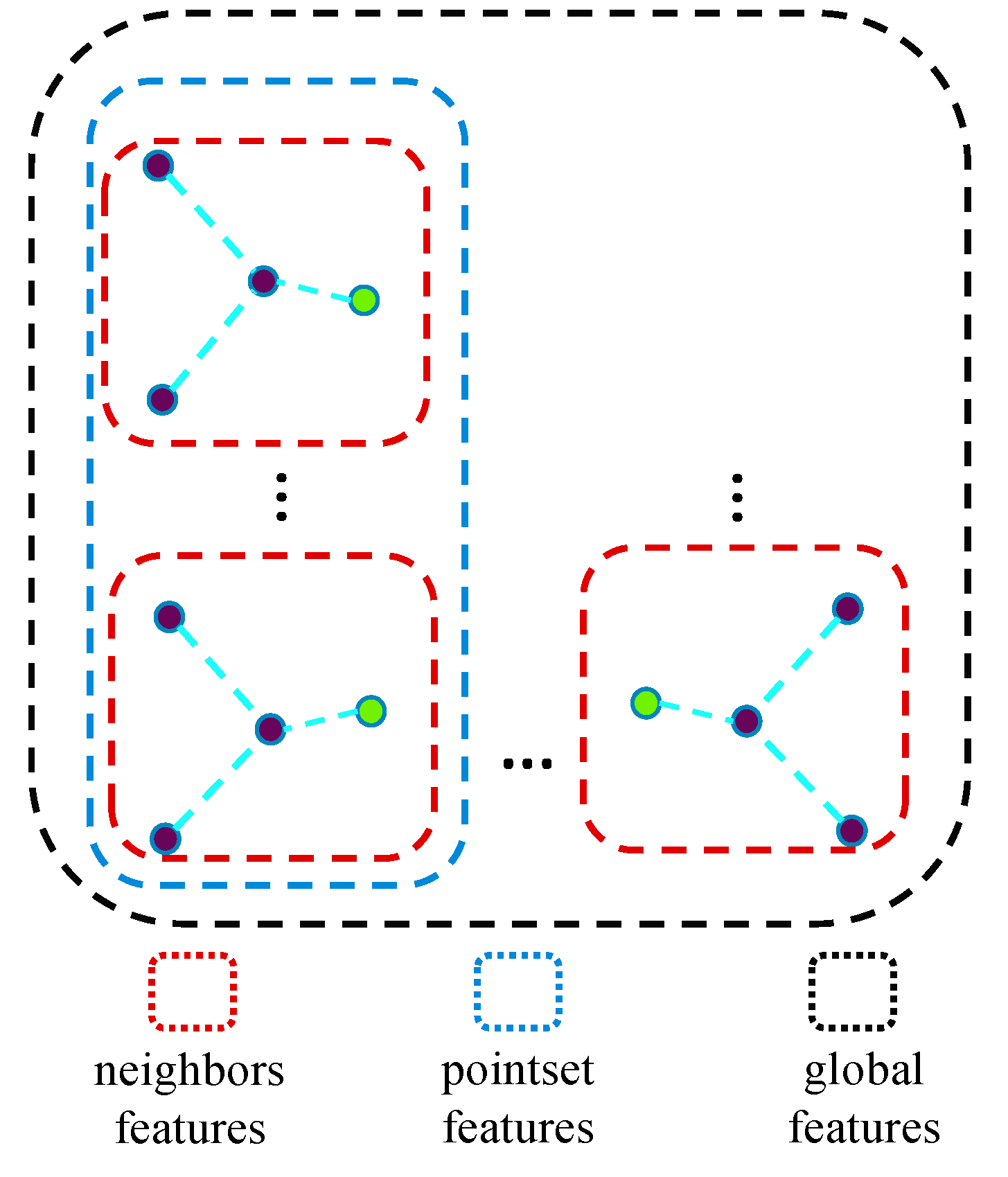
• We propose a new module MEFL that extends the GAPLayer to extract features at three different scales, namely, single point scale, point neighborhood scale, and pointset scale, enabling the network to extract multi-granularity features of point clouds.
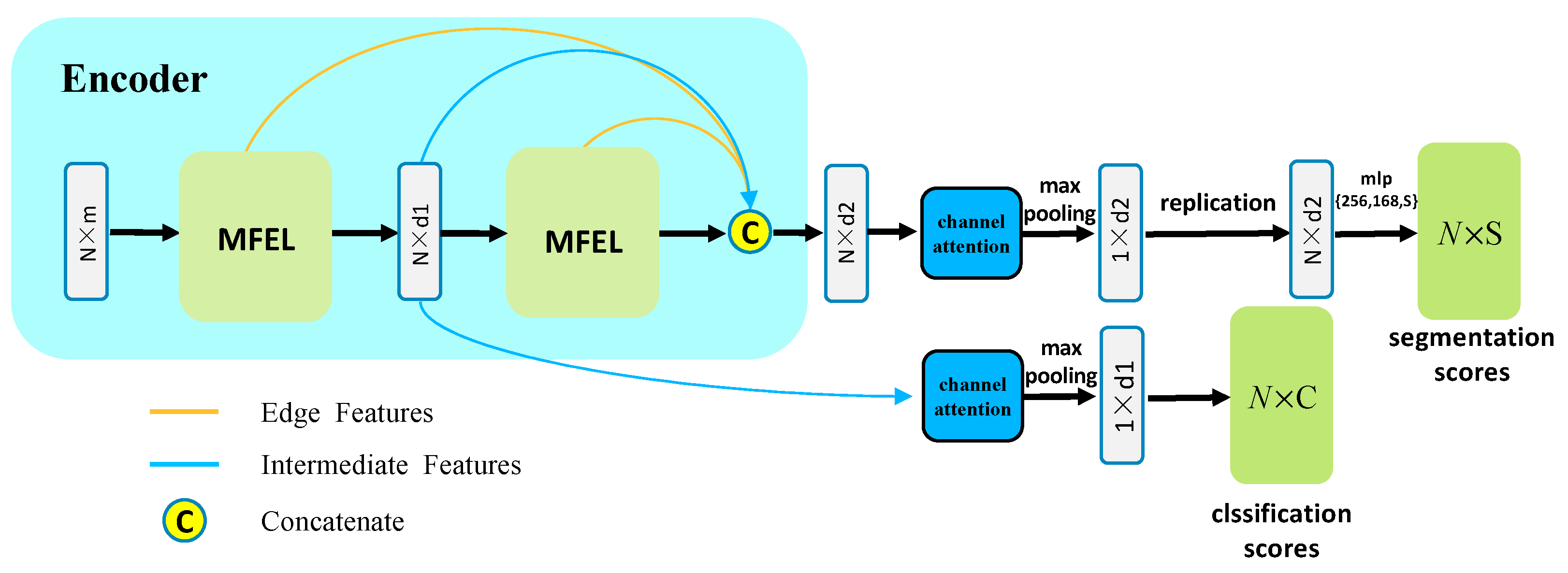
• We introduce an end-to-end framework named the multi-level feature fusion neural network (MFNet) for the tasks of classification and part segmentation, which effectively fuse features of different scales and levels.
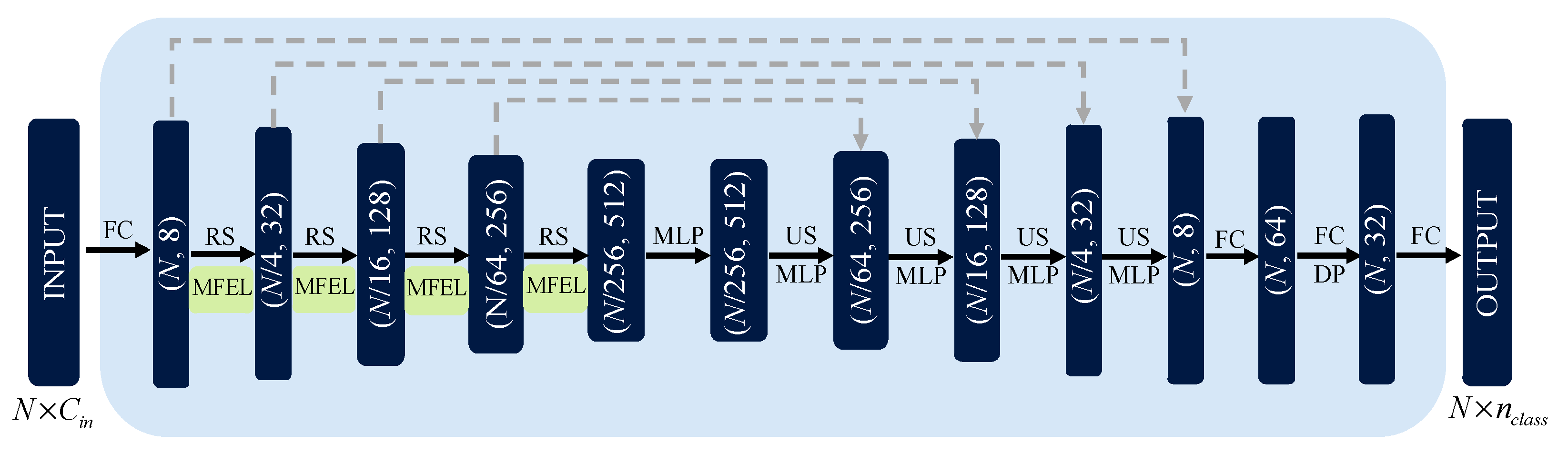
• Furthermore, we design a network MFNet-S for semantic segmentation tasks and conduct comparative experiments on large indoor and outdoor datasets.

The remainder of this paper is organized as follows. Section 2 reviews the related work. Section 3 gives the details of the proposed methodology. Section 4 introduces the setting of the experiments, the datasets (including ModelNet40 [14], ShapeNet [15], S3DIS [16], and Sementic3D [17]), and discusses the experiment results. Section 5 summarizes our research.

2. Related Work

In this section, we briefly summarize related work on point cloud processing, including deep learning-based frameworks, attention mechanisms, and feature representation methods.

2.1. Deep Learning-Based Methods for Point Cloud Processing

Deep learning-based point cloud processing methods can be classified into two categories according to the input form, namely, regularized input and input that is direct from the original point clouds.

2.1.1. Regularized Representation

Regular data (such as images) can easily extract context features by using a shared convolution kernel. Thus, one approach to process a point cloud by CNN is to transform the point cloud to the regularized form. Voxelization and multi-view projection are two common regularization methods.

Voxelization is to represent the point clouds with regular 3D voxel grids, and each grid represents a spatial unit. For example, VoxNet [6] uses a supervised 3D CNN-based occupancy grid to extract voxel features. The computational cost of voxel-based models increases dramatically with increasing resolution. To reduce the computational and memory overhead, Wang et al. [18] used an unbalanced octree to divide the space hierarchically, so that computational resources are concentrated on content-dense regions.

Another method is to project the point cloud onto the planes of multiple views and express 3D point cloud information using 2D images of the multiple planes. The challenge of this approach is how to efficiently aggregate features from multiple views. For example, GVCNN introduces a grouping strategy to consider the content relationship and discrimination between views, and then the group level features are aggregated into the shape descriptor according to their discriminative weights [7]. Ma et al. used long short-term memory and a sequence voting layer to aggregate view-wise features into a shape descriptor [8]. The multi-view method only preserves 2D information within a limited number of perspectives and has relatively high computational efficiency [19]. It is often used for classification or retrieval tasks. However, due to the loss of geometric information in the projection process, the performance of semantic segmentation in large-scale scenes needs to be improved further. To reduce the quantization loss after projecting, ASCNet [20] employs a module named PSCFE (pillar-wise spatial context features encoding) before projecting, which can capture the context features as vertical-wise within the pillars and the neighborhood geometric information between pillars.

2.1.2. Direct Representation of Original Point Clouds

Point cloud data are unordered and unstructured. Thus, it is not feasible to directly apply CNNs to point clouds. In order to reduce the loss of information and directly process point clouds, some researchers have proposed a series of point-based frameworks, and these works can be roughly divided into point-wise MLP methods and graph-based methods.

(1) Point-wise MLP methods. PointNet [9] is a pioneering work of applying deep learning directly on point clouds. Specifically, it applies the MLP on each point, and then uses the max-pooling to aggregate features of all points to achieve permutation invariance. PointNet is computationally efficient, but its learning process aims to encode each point individually, regardless of the contextual relationship between points. PointNet++ [10] is an extension work of the PointNet. It hierarchically samples and groups the input and applies the PointNet pipeline on each group. Then, the features of the local region are aggregated into the centroid as local features. PointNet++ still encodes each local point independently, which makes it hard to utilize the local geometric information. To capture the local patterns better, KPconv [12] proposes the kernel point convolution. It uses the kernel function to calculate the weight matrix of the points that fall within the range of a sphere, and the matrix is used to transform the features of this point. Aggregating the neighborhood features of points onto a point inspired us to construct local neighborhood graphs and gather the graph features to the central point. To further capture additional local geometric information, PointVGG [21] defines operations of convolution and pooling, i.e., Pconv and Ppool, respectively. The Pconv could pay attention to the relations between neighbors, and the Ppool makes the network abstract the underlying shape information. LGS-Net [22] proposes a local geometric structure representation block to model fine-grained geometric structures by fully utilizing relative and global geometric relationships in the neighborhood.

(2) Graph-based methods. This kind of approach attempts to process non-Euclidean structured data (e.g., 3D point clouds or social networks) through deep neural networks [23,24]. Relevant works on graph convolution can be divided into spectral-based and non-spectral (or spatial)-based methods [25].

Spectral-based graph neural networks perform Fourier transformation and eigen decomposition in the Laplace matrix of the graph. The spectral convolution can be defined as the element-wise product of Fourier variations of two signals on the graph [26]. For example, Yi et al. [27] parametrized the convolution kernel in the spectral domain and constructed a spectral conversion network to share the network parameters. The disadvantage of spectral-based graph CNN methods is that the entire point cloud needs to be loaded into memory for graph convolution. Since the Laplacian matrix eigen decomposition is time-consuming, the spectral-based CNNs consume a lot of computational resources. To solve this problem, Defferrard et al. [28] reduced the computational complexity through the Chebyshev polynomials and their approximate calculation scheme. Furthermore, Wang et al. [29] designed graph convolution on local pointsets and applied recursive clustering and pooling operations to gather spectral information from neighboring nodes to reduce computation. Spectral-based methods can effectively capture the local geometric features. This also means that the feature construction method based on a graph may directly affect the feature extraction.

Spatial-based graph neural networks usually define a neighborhood to perform graph convolution operations on the spatial relationships of nodes within the neighborhood. For instance, Duvenaud et al. [30] computed local features by summing the weight matrix of adjacent vertices and multiplying by its neighboring nodes, thus sharing the same weights between all edges. DGCNN [31] applies convolution to each edge where the local neighborhood is connected to the query points and dynamically updates the graph. Wang et al. [26] introduced a graph attention convolution (GAC) that assigns different attention weights to different neighboring points according to local information. Thus, the kernel of GAC can adjust dynamically to accommodate different objects with different structures.

2.2. Attention Mechanism

In recent years, an attention mechanism has been used to spotlight the important parts of features [32]. In order to adaptively adjust the weights between channels, SENet [33] builds feature maps with the help of the inter-channel correlations. The GATs [34] can assign different weights to different neighboring nodes in graph convolution operations. RandLA-Net [3] takes a similar strategy to SENet in each neighborhood. That is, neighbor features are fed into a shared MLP followed by softmax to generate attention scores. Then, the neighbor features are weighted summed according to the score to update the center point features. The difference is that RandLA-Net produces edge weights without dimension compression. SCF-Net [35] has improved RandLA-Net in the attention mechanism. Specifically, SCF-Net introduces the distance of geometric space and feature space in addition to the neighbor feature itself to generate the attention coefficient. This allows the attention coefficient to contain more information.

A point transformer [36] introduces the self-attention transformer based on the encoding decoding structure in the NLP (natural language processing) field into the point cloud processing field, and it has achieved remarkable results. However, Zhang et al. [37] proposed that the calculation cost of existing point transformers is very high because they need to generate a large attention map. Therefore, they proposed Patch attention (PAT) to adaptively learn a much smaller set of bases and calculate attention mapping on this basis.

Inspired by these methods, our model learns the attention weight of each edge in the graph structure through the neighborhood features, to extract local features, so that the model can focus on the edge features in the neighborhood and better facilitate semantic understanding. In addition, SENet is used to filtrate the fused multi-level features to highlight important parts and suppress redundant features.

2.3. Feature Representation Methods

Many feature descriptors are designed based on human experience in point cloud processing. For example, Salti et al. [38] proposed signatures of histograms of orientations (SHOT), which use local histograms to extract descriptors on the surface of an object. This descriptor is similar to the classic spin image [39], point feature histograms (PFH) descriptor, and fast point feature histograms (FPFH) descriptor [40], etc. However, these feature descriptors rely on the stable surface information acquisition of objects, which limits their broad applications. Arandjelov et al. [41] proposed NetVLAD, which converts non-differentiable functions in VLAD vectors [42] into differentiable functions in a clever way. It successfully applies BoF-based (bag of feature) [43] feature descriptors to deep learning networks. Further, PointNetVLAD [44] combines PointNet with NetVLAD to build an end-to-end model of point cloud retrieval.

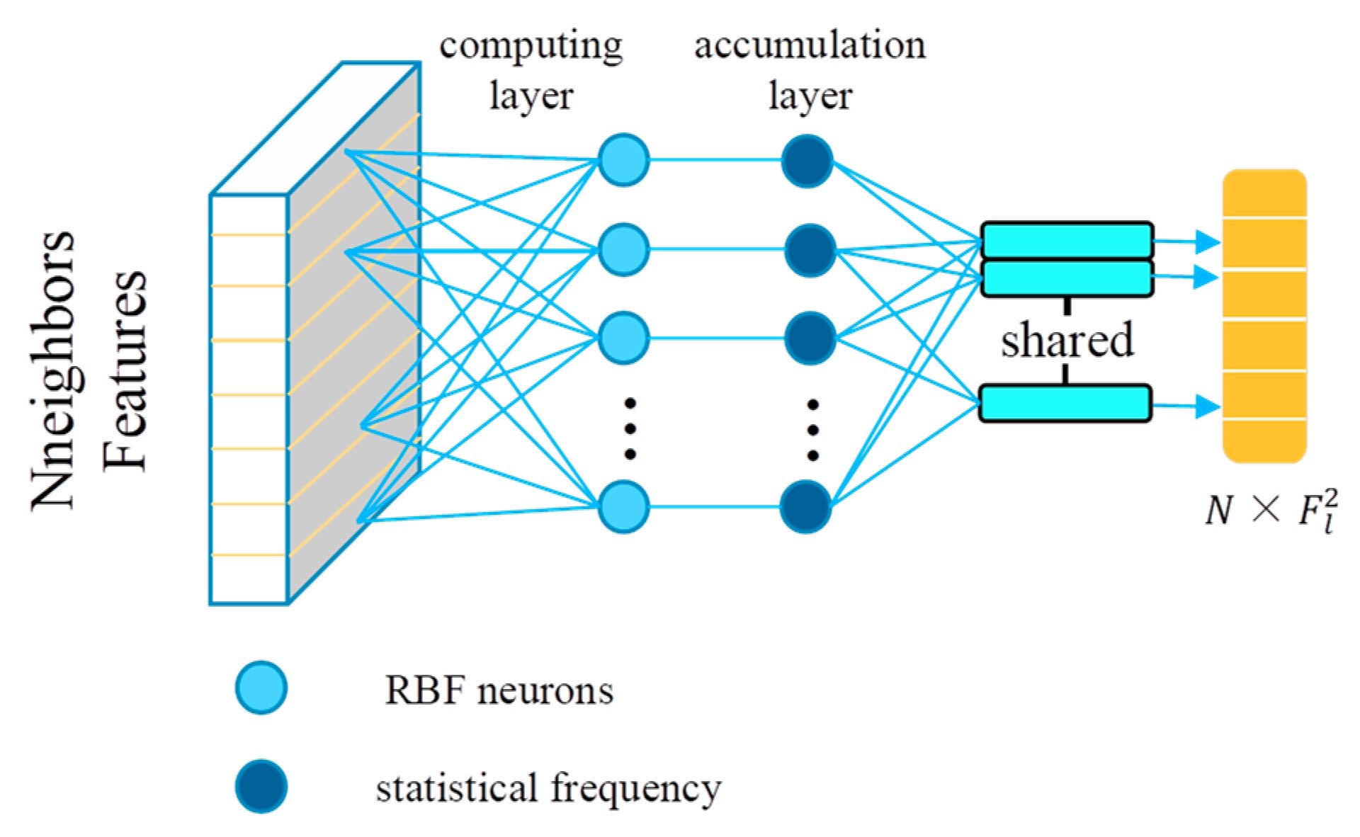
In order to make our feature extraction module more robust, similar to the feature descriptor construction process of VLAD, this research uses the radial basis function (RBF) to learn cluster centers to extract pointset level features.

3. Methodology

In this section, we introduce the MFEL and our network architecture for point cloud classification and segmentation. As show in Figure 3, MFEL exploits the aggregated GAPLayer, spatial position perceptron (SPP), and RBFLayer to capture more complete geometric features of 3D point clouds.

The aggregated GAPLayer and the SPP are two parallel branches, which directly extract features from the input (original input or feature maps). The aggregated GAPLayer uses the K-nearest neighbors (KNN) to find the respective neighborhood for each point and extract the local geometric features from each neighborhood, since the local geometric features contain contextual information that is more conducive to describe the similarity between pointsets. Thus, the local geometric features are fed into the RBFLayer to obtain the enhanced local features to distinguish the features of pointsets. The SPP is designed to extract features at a global level.

3.1. Aggregated GAPLayer

The GAPLayer only extracts geometric features in the local coordinate system of ② or ③ in Figure 1. To address this problem, we propose the aggregated GAPLayer, which contains an aggregated coordinate channel to associate the local coordinate system with the world coordinate system shown in ① in Figure 1.

As shown in Figure 4, the input of the aggregated GAPLayer is $I_l=\left\{x_1,x_2,\dots ,x_N\right\}\in {ℝ}^{N\times C_l^{in}}$, where N is the number of the input point clouds, and $C_l^{in}$ is the number of input channels of the l-th MFEL. The local structure of the point cloud can be denoted as a directed graph $G=\left(V,E\right)$, where $V=\left\{v_1,v_2,\dots ,v_N\right\}$ is the set of N point nodes, and $E\subseteq N\times N$ are edges of a local graph. We employ KNN to construct G in the feature space. Edge features $y\left(x\right)$ can be calculated as $y_{ij}=x_i-x_{ij}$, where $i\in V$, and $j\in k$, and k is the number of neighbors.

The edge features $y\left(x\right)$ contain the geometric structure information of the neighboring points corresponding to the query point. Then, we apply a shared convolution kernel to $y\left(x\right)$ to extract the depth-level local geometric edge features $y^{\prime }\left(x\right)$. Assuming that $y\in {ℝ}^{N\times k\times C_{in}}$, ${y^{\prime }}_{ij}$ can be calculated as follows:

$${y^{\prime }}_{ij}=(y_{ij}·{\mathit{W}}_l^{C_{in}\times C_l^1}+\theta )\subseteq {ℝ}^{N\times k\times C_l^1},$$

(1)

where W is the parameters of the shared convolution kernel, l represents the l-th MFEL, and θ is a bias term. Equation (1) can be represented as ${y^{\prime }}_{ij}=h\left(y_{ij},\theta \right)$. That is, we want to find a nonlinear function $h(\cdot )$ with at least $C_{in}\times C_l^1$ parameters, which can map edge features to a high-dimensional space. The effects of the values of k will be discussed in the Section 4.

In addition, each edge has a different contribution to the representation of local geometry. As shown in Figure 5, there are strong dependencies between neighboring points (i.e., $x_{i1}$ or $x_{i2}$) and center point $x_i$, which belong to the “wing”. Thus, the model should pay more attention to the edges $y_{i1}$ and $y_{i2}$, while ignoring the edge $y_{i3}$ and connecting the “fuselage” point. This varying degree of dependency is influenced by both the central point and the neighboring points. Therefore, we design an attention pooling layer to learn the nonlinear interaction from the perspective of the central point and neighboring points, respectively. The pooling layer is constructed by self-attention channels and neighbor-attention channels. Specifically, the self-attention layer uses the convolution kernel without bias to extract the spatial information of the query point itself and generate the self-attention coefficient. Then, the neighbor-attention layer uses a nonlinear function to extract the neighbor-attention coefficient from the edge features. To fuse these two attention coefficients, we employ a simple sum function. Finally, the fused coefficients are normalized to generate a weight $\widehat{{\alpha }_{ij}}$ for each edge as shown in Equation (2).

$$\widehat{{\alpha }_{ij}}=\frac{{\alpha }_{ij}}{{\sum }_{k\in N_i}{\alpha }_{ik}}\subseteq {ℝ}^{N\times 1\times k},$$

(2)

where ${\alpha }_{ij}=\sigma \left(h\left(x_i\right)+h\left({y^{\prime }}_{ij},\theta \right)\right)$ is the edge weight before normalization, and $\sigma (·)$ is the activation function. Here, the LeakyReLU was chosen. The weighted edge features $\widehat{{y^{\prime }}_{ij}}$ are calculated as follows:

$$\widehat{{y^{\prime }}_{ij}}=\widehat{{\alpha }_{ij}}\times {y^{\prime }}_{ij}\subseteq {ℝ}^{N\times C_l^1},$$

(3)

To better describe the contextual information of a local region, we add a channel to GAPLayer to aggregate the absolute position information of the neighborhood relative to the entire point cloud. We apply a set of shared convolution kernels on each point in the neighborhood and aggregate the feature ${x^{\prime }}_{ij}$ of each point with a pooling layer:

$${x^{\prime }}_{ij}=Max\left\{h\left(h\left(x_{ij}\right)\right)\right\}\in {ℝ}^{N\times C_l^2},$$

(4)

where the function Max{∙} means max-pooling function. Then, ${x^{\prime }}_{ij}$ is concatenated with the attentive edge feature $\widehat{y^{\prime }}$ as shown in Equation (5):

$$E=[\widehat{y^{\prime }}\Vert x^{\prime }]\in {ℝ}^{N\times F^1},$$

(5)

where the $F^1=C_l^1+C_l^2$ is the final output dimension of the proposed module.

3.2. RBFLayer

As shown in Figure 2, pointsets with similar geometric structures usually have similar spatial distribution characteristics. Such a pointset often has a large spatial range, and its distribution characteristics are less affected by noise, which can express the characteristics of objects more comprehensively.

The radial basis function (RBF) only responds to the distance between the input variable and the center point, and the response is monotonic. Therefore, it is suitable to describe the distribution of points in space. The RBF can be defined as:

$$\phi \left(x,v\right)=\phi (\Vert x-v\Vert ),$$

(6)

where x and v are the input and center, respectively. We expect the points in the pointset to have similar characteristics. Thus, a kernel function whose output is inversely proportional to the distance (namely, ‖x − v‖) is designed, e.g., the Gaussian function:

$$k\left(x,v^{\prime }\right)=\exp (-\frac{{\Vert x-v\Vert }^2}{2{\delta }^2}),$$

(7)

where δ is a hyperparameter that adjusts the width of the Gaussian function. Such RBF can well reflect the spatial distribution in a large range, and the distribution characteristics are explicitly modeled. Inspired by the RBF, we propose a pointset feature extraction module called the RBFLayer, which can extract pointset features that contain richer context information. In addition, the feature extraction method based on point clusters can aggregate some scattered points into an overall representation. Therefore, the RBFLayer can extract statistical features and reduce the influence of point density changes.

In our work, the RBF is used as a feature extractor to generate statistical features in the scale of the pointset. The intermediate features are fed into the RBFLayer to model the distribution in the feature space. Specifically, the RBFLayer learns a predetermined number of cluster centers from the feature maps. As shown in Figure 6, the RBFLayer consists of two sub-layers, namely, the computing layer and accumulation layer.

Assuming that the extracted feature map has N feature vectors, $x_i\in R^F\left(i=1,\dots ,N\right)$, the computing layer calculates the similarity between the input feature vectors and the feature vectors of cluster centers. Then, the results of the computing layer are sent to the accumulation layer. The accumulation layer quantifies the similarity into a histogram. To normalize the output, we use Equation (8) as the kernel function:

$${\left[\phi \left(x\right)\right]}_t=\frac{exp\left(-{\Vert x-v_t\Vert }_2/{\delta }_t\right)}{{\sum }_{q=1}^{N_t}exp\left({\Vert x-v_q\Vert }_2/{\delta }_t\right)},$$

(8)

where v is a learnable cluster center with the same dimension as the input vector. The output $s_j$ of the accumulation layer is calculated as follows:

$$s_j=\frac{1}{N_i}{\sum }_{j=1}^t\phi \left(x_{ij}\right),$$

(9)

where $\phi (x_{ij}$) is the output of the i-th feature $x_i$ on the j-th radial neuron. The RBFLayer outputs the statistical histogram of the entire point clouds, denoted as $S=\left(s_1,s_2,\dots ,s_t\right)$. Finally, S replicates N times to concatenate with the output of the aggregated GAPLayer.

3.3. Spatial Position Perceptron

To enrich the feature hierarchy, another module is introduced, i.e., the spatial position perceptron (SPP), to extract the global features of the whole point clouds. As shown in Figure 7, the SPP can obtain a larger receptive field than a pointset consisting of K-nearest neighbors. All points are directly fed into the shared convolutional layer, and the interconnection between all points is established to form the global feature of the entire point cloud. The global features are denoted as U:

$$U=h\left(x_i,\theta \right)\in {ℝ}^{N\times F^2},$$

(10)

In the aggregated GAPLayer mentioned in Section 3.1, we use a similar method on the neighborhood with k points. The difference is that the aggregated GAPLayer just aggregates the spatial information in a local region, and the SPP is concerned with all input data. We note that some related works embed raw coordinates (x, y, z) into each feature extraction layer. Our purpose is to make the model learn the location information of points in different dimensions in the space. Therefore, the input of the first MFEL is the raw coordinates, while the input of the second MFEL is the feature maps output by the previous MFEL, and so on.

3.4. The Proposed MFNet and MFNet-S

As shown in Figure 8, an end-to-end point cloud classification network, namely, MFNet, is constructed based on the MFEL. The MFEL is used to extract features of three different scales, including neighborhood features, pointset features, and global features, as shown in Figure 2. In the part segmentation network, the middle-level features and the deep-level features are also connected by means of the skip connection. Finally, the multi-scale and multi-level semantic features are extracted.

3.4.1. Classification Network

As shown in the bottom pipeline of Figure 8, to keep the results robust to the changes of the input (such as rotation, zoom, etc.), our classification and part segmentation networks implement the spatial transformation network, and the classification network uses one MFEL as an encoder. As the geometric structure information in a neighborhood is abundant and the information collected by one neighborhood feature extraction module is limited, we adopt the multi-head mechanism to learn more information independently by using the aggregated GAPLayer in different subspaces. Then, the outputs of multi-heads are concatenated. We set the head number h = 4 and the neighboring point number k = 20 in the classification network. The channel-attention mechanism SENet is used to assign weights to the merged feature channels. Finally, we apply three fully connected layers with drop-out to convert the global features obtained by max-pooling into classification scores of 40 categories. Furthermore, each fully connected layer is nonlinearly transformed with the help of the batch normalized activation function ReLU.

3.4.2. Part Segmentation Network

As shown in the top pipeline of Figure 8, the part segmentation task requires richer context and deeper information. Thus, the part segmentation network sets k = 30 and uses two MFELs. As the network depth and neighbor nodes increase, the consumption of computing resources also increases. Thus, we reduce the number of heads, and set h = 2. The output intermediate features of the first MFEL are fed into the second MFEL. Then, the salient edge features in each MFEL with the output of the two MFELs are concatenated and fed into the SENet. We use the tiling function to restore the pooled features to the feature size before pooling. Finally, the fully connected layer is used to generate the prediction score for each point. In this research, the cross-entropy loss is used in classify training.

3.4.3. Semantic Segmentation Network

In the task of semantic segmentation, the MFEL is embedded in the U-Net framework, namely, MFNet-S, as shown in Figure 9. The input is fed to the encoder after the fully connected layer. The encoder consists of four down-sampling layers. Each layer equips an MFEL with two heads to extract the multi-level features. As the number of points decreases, the feature channel dimension is continuously increased. The output of the last down-sampling layers is directly fed into the first up-sampling layer of the decoder. The decoder consists of four up-sampling layers, and the up-sampling algorithm is the nearest neighbor interpolation. Additionally, the skip connection is used to concatenate the features of the same size between the encoder and decoder. The final semantic label of each point is obtained through three shared fully-connected layers and a dropout layer. The dropout ratio is 0.5. The output is the predicted semantics of all points with a size of $N\times n_{class}$, where $n_{class}$ is the number of classes. Furthermore, the cross-entropy loss is used to train the model.

4. Results and Discussion

To verify the effectiveness of the proposed algorithm, we perform a qualitative and quantitative analysis of the proposed algorithm on four indoor and outdoor point cloud datasets. We first conduct ablation study experiments on the ModelNet40 to verify the effectiveness of each part of the MFEL. Then, we implement the MFNet to conduct the part segmentation experiments on the ShapeNet. Finally, the MFNet-S is used to perform semantic segmentation experiments on different point cloud datasets. The comparisons and analysis for the experiments are also provided.

4.1. Datasets

ModelNet40: The ModelNet40 is a synthetic dataset. Compared with the real datasets collected by laser scanning, each object in the ModelNet40 has a complete shape and does not contain noise. The ModelNet40 has 40 common man-made categories, such as cups, hats, and chairs, and contains 12,311 objects in total. We use about 80% (9843) for training and the remaining 20% (2468) for testing.

ShapeNet: The ShapeNet is also a synthetic dataset. The ShapeNet contains 16 categories and 16,881 samples. Each sample contains 2–5 parts, such as an aircraft contains 4 parts, namely, fuselage, wings, engines, and tail. All objects have a total of 50 different parts. As usual, we use 80% of the samples as training data and the remaining 20% as test data.

S3DIS: The S3DIS is a large-scale indoor point cloud dataset developed by Stanford University. The S3DIS is reconstructed from six large indoor areas (Area 1–Area 6) scanned by Matterport camera. The S3DIS is further divided into 271 rooms. Each point in the dataset is semantically labeled by one of the 13 common indoor objects, such as chair, table, and floor. Each point is represented by a 9-dimensional vector, i.e., X, Y, Z, R, G, B, and the normalized X, Y, and Z. Note that the normalized coordinates X, Y, and Z are between 0 and 1.

Semantic3D-8: The Semantic3D is a large-scale outdoor scene dataset scanned by terrestrial laser scanning. The Semantic3D contains different natural and artificial scenarios such as rural areas, sport fields, and urban squares. Each scene contains tens of millions of points, with a total of more than one billion points for the whole dataset. The Semantic3D-8 has 8 categories, such as plant, building, vehicle, etc. Each point contains 3D coordinates, R/G/B color information, and intensity. Compared with the above dataset and indoor dataset, its density distribution is more uneven. The Reduce-8 training set is the same as the Semantic3D-8, but the test set is a uniformly down-sampled sub-dataset with an interval of 0.01 m.

4.2. Evaluation Metrics

On the ModelNet40, we employ overall accuracy (OA) and mean class accuracy (mAcc) as our classification task evaluation indicators. If we suppose l is the number of categories (the number of labels in the semantic segmentation task), OA is calculated as follows:

$$OA=\frac{{\sum }_{i=0}^l{P}_{ii}}{{\sum }_{i=1}^l{\sum }_{j=1}^l{P}_{ij}},$$

(11)

where $P_{ij}$ represents the point predicted to be of class j but actually of class i. The OA reflects the overall classification ability of the network, as it represents the proportion of the number of correctly classified samples to the total number of samples. However, sample balance may affect the OA value and reduce the generalization of the network. mAcc calculates the OA value of the prediction results for each class of objects, and then averages the OA values of all classes:

$$mAcc=\frac{1}{l}{\sum }_{i=0}^l\frac{P_{ii}}{{\sum }_{j=0}^l{P}_{ij}},$$

(12)

For the ShapeNet, S3DIS, and Semantic3D, the evaluation metrics are the same as most of the references to facilitate the comparison of experimental results. Here, mIoU (mean IoU) and mAcc are used on the ShapeNet. OA and mIoU are used on the S3DIS and Semantic3D. The $Io{U}_i$ is calculated as follows:

$$Io{U}_i={\sum }_{i=1}^l\frac{P_{ii}}{{\sum }_{j=1}^l{P}_{ij}+{\sum }_{j=1}^l{P}_{ji}-P_{ii}},$$

(13)

The mIoU evaluates the semantic segmentation results for all classes, which are calculated by Equation (14):

$$mIoU=\frac{1}{l}{\sum }_{i=0}^l\frac{P_{ii}}{{\sum }_{j=1}^l{P}_{ij}+{\sum }_{j=1}^l{P}_{ji}-P_{ii}},$$

(14)

4.3. Ablation Studies and Parameter Sensitivities Analysis

In this section, we conduct ablation experiments on the MFNet by comparing it with the GAPNet. We also conduct sensitivity experiments on several key hyperparameters. These experiments are conducted on RTX 2080Ti with Tensorflow v1.12.

4.3.1. Ablation Studies

The training parameter settings are the same as the GAPNet: 1024 points as the input, learning rate = 0.001, and training epoch = 250. Data augmentation operations include random rotation and jitter. For optimization, we use Adam to train the model for 250 epochs with batch size = 32. The initial learning rate is set to 0.001. We will sequentially add our proposed modules into the GAPNet. The experimental steps are as follows.

Step 1: The feature extraction module GAPLayer in the GAPNet is replaced by our improved aggregated GAPLayer. The MLP channel numbers in SPP are 8, 16, and 16, respectively. Step 2: The RBFLayer is added to the network after step 1. Here, we choose the number of RBF neurons t = 40. Step 3: The spatial position perceptrons with convolution channels of {32, 64, 64} are added to the network after step 2. Step 4: We embed the SENet channel-attention mechanism into the network. The attention coefficients for all feature channels can be assigned according to the feature map, to highlight significant features and suppress redundant features.

The experimental results of the ablation studies are shown in

Table 1. Ablation studies on ModelNet40 dataset.

Component	Base Model	Step 1	Step 2	Step 3	Step 4
GAPLayer	√
Aggregate GAPLayer		√	√	√	√
RBFLayer			√	√	√
Spatial Position Perceptron				√	√
SENet					√
OA (%)	92.4	92.5	92.6	93.0	93.1
mAcc (%)	89.7	90.4	90.6	90.9	91.4

Note: “√” means that the module has been added to the network. In all tables in this article, bold font indicates best results.

. With the addition of modules, the OA and mAcc show an upward trend, indicating that each module has played an active role. When all modules are loaded, the proposed MFNet is formed. OA and mAcc reach 93.1% and 91.4%, respectively, which are 0.7% and 1.7% higher than the original GAPNet, respectively. Further comparison can find that the improvement of mAcc in step 1 is the largest, which is increased by 0.8%, and the improvement of OA in step 4 is the largest, which is increased by 0.4%. This proves that for small-scale point cloud classification tasks, adding rich geometric features and global features can help the network to distinguish object categories more accurately.

4.3.2. Parameter Sensitivities Analysis

We conduct parameter sensitivity experiments in the classification and segmentation networks of the MFNet, respectively. The training strategy of parameter sensitivity analysis in the classification network is the same as the ablation experiments. In this experiment, we discuss the influence of neighboring point number k and RBF neuron number t on the classification results. According to

Table 2. Parameter sensitivity analysis on the classification network.

	t = 40			k = 20
	k = 10	k = 20	k = 40	t = 20	t = 40	t = 80
OA (%)	92.5	93.1	92.8	92.9	93.1	92.8
mAcc (%)	90.3	91.4	90.2	90.7	91.4	90.3

, when k = 20 and t = 40, the MFNet performs best on the ModelNet40. In addition, there is no obvious correlation between the neighboring point number or RBF neurons’ number with classification accuracy because the size of the neighborhood may affect the model’s perception of fine-grained geometric features. According to the experiments, the number of RBF neurons should be approximately equal to the number of categories in the dataset, which will make the RBF neurons describe the characteristics of the pointset best.

For the part segmentation task, each object is sampled with the 2048 point as the input. The initial learning rate is set to 0.005 with the Adam optimizer. The model is trained in 200 epochs with the batch size of 16. Since the part segmentation task is more sensitive to parameters, we further discuss the influence of the head number (h) and the number of output channels (C) of each aggregated GAPlayer on the results here. The RBF neurons (t) are set to 40. The results are shown in

Table 3. Parameter sensitivity analysis on ShapeNet dataset.

		$({\mathit{C}}_1^1, {\mathit{C}}_1^2)$	$({\mathit{C}}_2^1, {\mathit{C}}_2^2)$	mAcc (%)	mIoU (%)
head = 1	(1) k = 30	(64, 16)	(256, 128)	94.3	84.7
head = 2	(2) k = 40	(32, 16)	(128, 128)	94.5	85.4
	(3) k = 30	(32, 16)	(128, 128)	94.3	84.8
	(4) k = 30	(16, 16)	(128, 32)	94.1	84.6
	(5) k = 10	(32, 16)	(128, 128)	94.1	84.4
head = 4	(6) k = 30	(16, 16)	(128, 32)	94.4	84.8

Note: $C_l^1$ and $C_l^2$ mean the number of edge feature and local spatial aggregation feature output channels of the l-th module, respectively.

. By comparing configurations (3), (4), and (6), the three sets of experiments, it can be found that when k = 30, increasing the number of output channels can improve performance to a certain extent. Increasing the number of channels can compensate to a certain extent for the decrease in accuracy due to the reduction of the head number. On the other hand, reducing the head number will reduce the memory usage to further increase k to 40; the mAcc and mIoU of (2) are 0.1% and 0.6% higher than those in configuration (6), respectively. According to the comparisons of (1), (2), (3), and (4), we find that when the head number drops to 1, the expression capacity of the features cannot be improved even if the number of output channels is greatly increased. Thus, we finally choose the parameter setting of (2).

4.4. Comparison with Other Methods

To further verify the validity of the proposed model, in this section, we will make a detailed comparison of experimental results on four common datasets between our model and other methods.

4.4.1. Classification on ModelNet40

Table 4. Classification results comparing on ModelNet40 dataset.

Methods	OA (%)	mAcc (%)
PointNet [9]	89.2	86.0
PointNet++ [10]	90.7	-
DGCNN [31]	92.2	90.2
Point2Sequence [48]	92.6	90.4
A-CNN [11]	92.6	90.3
KPConv [12]	92.9	-
GAPNet [13]	92.4	89.7
LDGCNN [49]	92.9	90.3
PointASNL [50]	92.9	-
Point2Node [51]	93.0	-
Grid-GCN [46]	93.1	91.3
PointView-GCN [47]	95.4	-
HAPGN [2]	91.7	89.4
MFNet (ours)	93.1	91.4

Note: “-” means that the value of the item is not available.

shows the comparison results. Referring to the research [45], we divide the compared methods into three categories, i.e., point-wise MLP methods, convolution-based methods, and graph-based methods. In Table 4, our method achieves a remarkable performance on both OA and mAcc. Compared with graph-based methods such as Grid-GCN [46], our method achieves the same OA value, but we improve the mAcc value by 0.1%. Note that compared to the baseline (GAPNet), we improve 0.7% and 1.7% on OA and mAcc, respectively, despite the model size increase of 10 MB. In addition, for convolution-based methods, i.e., methods that focus on efficiently aggregating context within local regions, we also obtain competitive results over them. Compared to the KPconv, we lead by 0.2% in OA. In comparison with homogeneous methods (namely, the graph-based methods), our method has achieved remarkable results. For example, the PointView-GCN [47] is a state-of-the-art method, with an OA of 95.4%. However, the method has only been tested on small-scale datasets. Our method can be applied to semantic segmentation tasks on large-scale datasets as well as achieve remarkable results in the classification tasks on small-scale datasets.

4.4.2. Part Semantic Segmentation on ShapeNet

As shown in

Table 5. Part semantic results on ShapeNet dataset.

Methods	mAcc (%)	mIoU (%)
Kd-Net [52]	77.4	82.3
PointNet++ [10]	81.9	85.1
PCNN [53]	81.8	85.1
RS-Net [54]	81.4	84.9
KCNet [55]	82.2	84.7
DGCNN [31]	82.3	85.2
GAPNet [13]	-	84.7
Point-PlaneNet [56]	82.5	85.1
PatchFormer [37]	-	86.5
MFNet (ours)	83.2	85.4

, we divide the compared methods into four categories: structure-based, voxel-based, point-based MLP, and graph-based. Our method achieves the best mAcc and mIoU values among the four types of methods, reaching 83.2% and 85.4%, respectively. Compared with the baseline network, namely GAPNet, we improve mIoU by 0.7%. Experiments show that the feature extraction layer can extract semantic information very well in the task of part segmentation with a small amount of data. In comparison with homogeneous methods (namely the graph-based methods), our method has achieved the best results. The PatchFormer [37] achieves the best results on mIoU with 86.5%, but our method remains ahead on mAcc. In addition, the PatchFormer has also not been verified on large-scale datasets.

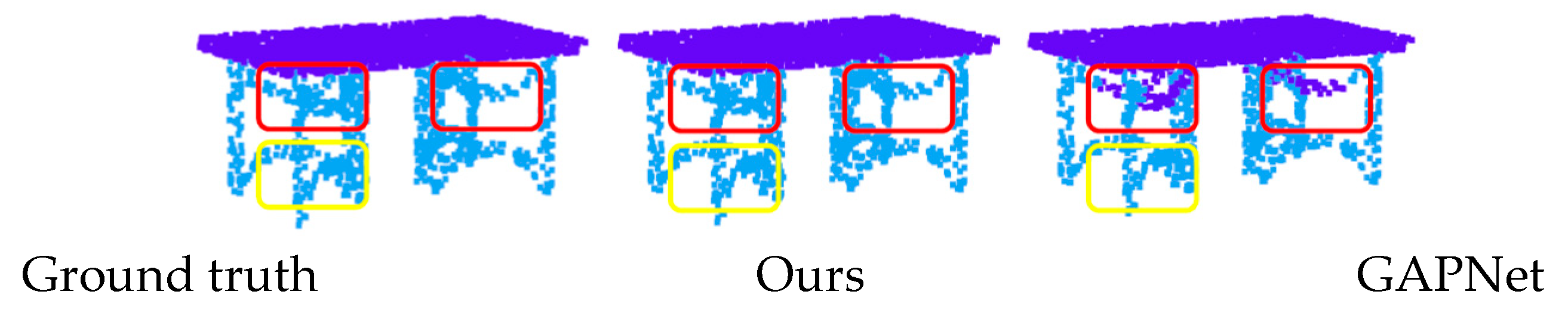
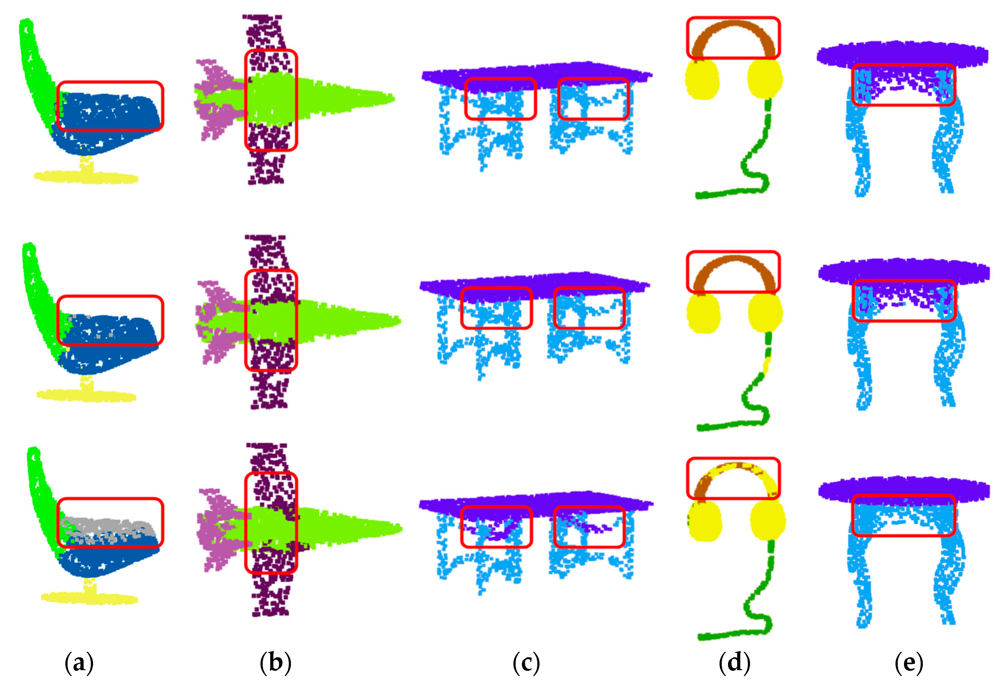
Figure 10 shows the visualization results of ShapeNet semantic segmentation. By comparison, it can be found that our method performs better on both flat and complex structures (such as red rectangles). Thanks to the geometric features extracted from the aggregated GAPLayer and pointset features of the RBFLayer, our network can better distinguish the shapes of various parts of the object, such as the armrest of the chair, the wing of the airplane, and the beam of the earphone. Since the RBFLayer can extract the object features of the pointset, when processing the object parts in Figure 10c, the connection between the upper and lower beams can be established, and the beams will not be erroneously segmented as with the GAPNet. However, our method incorrectly identifies a part of the line as the earmuffs, possibly because there is a gap in the line. Furthermore, the model mistakenly judges that the two parts separated by a certain distance are the earmuffs, as the distance between the misidentified part and the true earmuff is similar to the distance between the two true earmuffs.

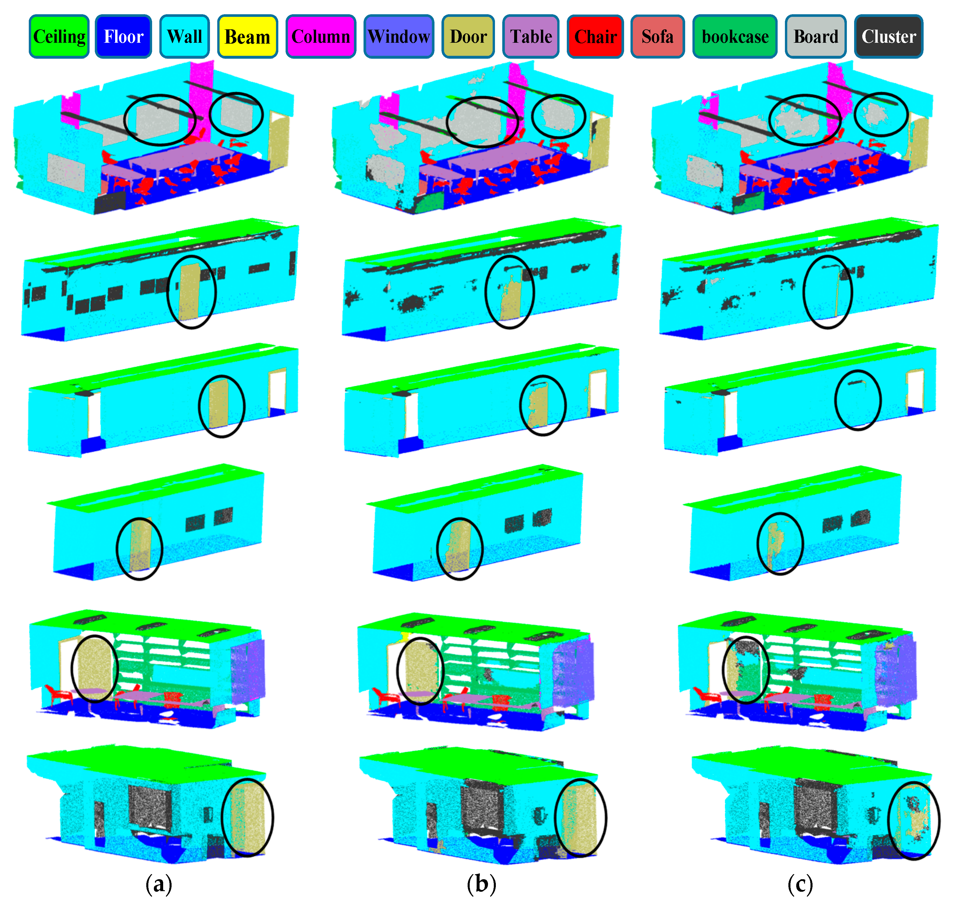
4.4.3. Semantic Segmentation on S3DIS

For the semantic segmentation task on the S3DIS and the Semantic3D, the MFNet-S network is employed. The Adam optimizer with an initial learning rate of 0.01 is used to train our model for 100 epochs. The batch size is set at 6 and 4, respectively, and the number of neighbors is set to 32 and 16, respectively, when training on the S3DIS and Semantic3D, and the decay rate of learning is set to 0.98. These two experiments are conducted on an NVIDIA Quadro RTX 6000 GPU.

Table 6. OA (%) and mIoU (%) on S3DIS dataset.

Method	OA	mIoU	Ceiling	Floor	Wall	Beam	Column	Window	Door	Chair	Table	Bookcase	Sofa	Board	Clutter
PointNet [9]	-	41.1	88.8	97.3	69.8	0.1	3.9	46.3	10.8	52.6	58.9	40.3	5.9	26.4	33.4
PointCNN [57]	85.9	57.3	92.3	98.2	79.4	0.0	17.6	22.8	62.1	74.4	80.6	31.7	66.7	62.1	56.7
TangentConv [58]	82.5	52.8	90.5	97.7	74	0.0	20.7	39.0	31.3	69.4	77.5	38.5	57.3	48.8	39.8
PointWeb [59]	87.0	60.3	92.0	98.5	79.4	0.0	21.1	59.7	34.8	76.3	88.3	46.9	69.3	64.9	52.5
HPEIN [60]	87.2	61.9	91.5	98.2	81.4	0.0	23.3	65.3	40.0	75.5	87.7	58.5	67.8	65.6	49.4
DGCNN [31]	59.8	51.5	93.0	97.4	77.7	0.0	12.2	47.8	39.8	67.4	72.4	23.2	52.3	39.8	46.6
GAPNet * [13]	85.7	59.4	89.1	97.0	79.4	0.0	28.8	57.6	35.3	76.0	80.0	50.9	66.2	63.2	48.3
Grid-GCN [46]	86.9	57.8	94.1	97.3	77.7	0.0	16.6	32.9	58.53	72.2	81.3	36.5	48.7	64.5	50.5
TGNet [61]	88.5	57.8	93.3	97.6	78.0	0.0	9.3	57.0	39.4	83.4	76.4	90.6	41.8	58.7	55.3
MFNet-S (Ours)	86.6	62.9	91.2	98.2	80.4	0.0	35.1	57.2	46.6	77.4	86.0	65.6	65.4	66.2	47.6

Note: Testing on Area 5 and training on the rest. Note that * is the result of replacing the feature extraction module of RandLA-Net with GAPLayer. Boldface indicates the method with the highest performance value.

provides the experimental results. The OA and mIoU of our method reach 86.6% and 62.9%, respectively, which are better than most compared methods. Compared with the GAPLayer, the OA and mIoU of our method are improved by 0.9% and 3.5%, respectively, and the segmentation results of each category are improved. Since our method integrates multi-scale features and can expand receptive fields, it has obvious advantages to segment large objects such as a column, bookcase, and board.

Compared with the local feature extraction network PointWeb, although the obtained OA is the same, the mIoU of our method is 2.5% higher, and it is better than the PointWeb in the segmentation results of most categories. In the graph-based approach (such as TGNet [61] and Grid-GCN [46]), our method takes the lead in both mIoU and mAcc.

Figure 11 shows the semantic segmentation visualization results of several typical scenes in the S3DIS. Compared with the ground truth and baseline model GAPLayer, our network has a strong recognition ability for large-area connected areas such as doors and window frames on the wall, and also has a good segmentation effect for objects with complex geometric structures (such as indoor furniture). This proves that the RBFLayer in our MFEL can better construct similar features of pointsets and can fully consider the geometric and spatial attributes of adjacent points. However, the boundary prediction of some large-area connection areas is not clear or complete. This is mainly because the limited receptive field limits its ability to learn geometric features to distinguish connected objects.

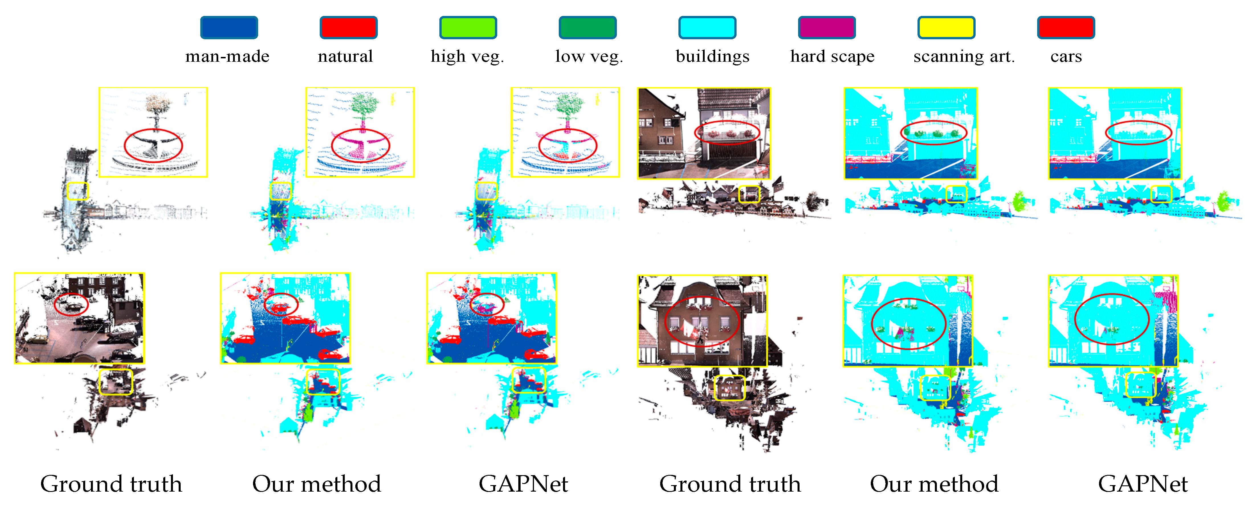
4.4.4. Semantic Segmentation on Semantic3D

For a fair comparison, we submit our prediction results on the Reduced-8 to the sever and evaluate the mIoU and OA.

Table 7. OA (%) and mIoU (%) on Semantic3d dataset (Reduced-8 test online).

Method	OA	mIoU	Man-Made	Natural	High vcg.	Low vcg.	Buildings	Hard Scape	Scanning Art.	Cars
PointNet [9]	-	41.1	88.8	97.3	69.8	0.1	3.9	46.3	10.8	52.6
GACNet [26]	91.9	70.8	86.4	77.7	88.5	60.6	94.2	37.3	43.5	77.8
SegCloud [62]	88.1	61.3	83.9	66.0	86.0	40.5	91.1	30.9	27.5	64.3
JSNet [63]	87.7	54.5	-	-	-	-	-	-	-	-
OFDV-Net [64]	88.3	57.3	86.5	75.4	76.1	40.3	89.2	14.0	27.9	49.2
OctreeNet [65]	89.9	59.1	90.7	82.0	82.4	39.3	90.0	10.9	31.2	46.0
XJTLU [66]	89.4	63.5	85.4	74.4	74.6	31.9	93.0	25.2	41.5	82.0
GAPNet * [13]	92.4	69.3	97.7	82.5	85.2	36.7	94.8	34.6	55.7	66.7
MFNet-S (Ours)	93.7	71.9	97.9	92.2	82.1	45.9	94.1	34.2	57.0	72

Note: the “*” is the result of replacing the feature extraction module of RandLA with GAPLayer. Boldface indicates the method with the highest performance value.

provides a quantitative comparison with several methods. The mIoU and OA of our network are 71.9% and 93.7%, respectively, which are significantly better than most existing methods. Compared with the baseline network, the results of our method are improved by 2.6% and 1.3%, respectively. The segmentation of our network in 4 of the 8 categories achieves the highest score in the compared methods. From the prediction results of the visualization in the real large-scale scene shown in Figure 12, our network can accurately segment small artificial objects such as carts and columns. The segmentation results on flat objects such as a sunshade surface are also complete. However, due to the sparse point cloud and the mixed geometric structure of the high vegetation leaves, the discriminative ability of the network is affected. Thus, our method is obviously inferior to the GAPNet in the recognition of targets such as high vegetation. This is what we will improve in the future.

Figure 11. Semantic segmentation visualization results on the S3DIS. (a) Ground truth; (b) our method; (c) GAPNet. As shown in the figure, the segmentation result of our method is better than that of GAPNet in the black circle.

Figure 11. Semantic segmentation visualization results on the S3DIS. (a) Ground truth; (b) our method; (c) GAPNet. As shown in the figure, the segmentation result of our method is better than that of GAPNet in the black circle.

5. Conclusions

In this research, we propose a new multi-scale feature extraction module MFEL for the large-scale point cloud classification. The MFEL first strengthens the local geometric feature extraction capability by adding a multi-layer perceptron channel with pooling layers to the graph convolution. Then, the statistical features of the point clouds at the pointset level are obtained via the RBFLayer. Finally, we combine the spatial location features extracted by the PointNet and design an end-to-end framework for the classification and part segmentation with better results. We also embed the module into a basic framework and perform experiments on large-scale indoor and outdoor point clouds, i.e., S3DIS and Semantic3D, with promising results. By the comparisons on several different types of datasets, our proposed feature extraction module provides greater improvements to the baseline model on large-scale datasets. In large-scale real scenarios, our proposed multi-scale feature extraction is more accurate and a stronger semantic representation for objects with rich geometric shapes.

However, our method is still inadequate in the segmentation of some small objects with complex structures, and inefficient feature fusion may lead to feature redundancy. Therefore, improving the efficiency of feature fusion and enriching the extraction of geometric features will be our future research.

References

1. Mi, X.; Yang, B.; Dong, Z.; Liu, C.; Zong, Z.; Yuan, Z. A two-stage approach for road marking extraction and modeling using MLS point clouds. ISPRS J. Photogramm. Remote Sens. 2021, 180, 255–268. [Google Scholar] [CrossRef]
2. Chen, C.; Qian, S.; Fang, Q.; Xu, C. Hapgn: Hierarchical Attentive Pooling Graph Network for Point Cloud Segmentation. IEEE Trans. Multimed. 2020, 23, 2335–2346. [Google Scholar] [CrossRef]
3. Hu, Q.; Yang, B.; Xie, L.; Rosa, S.; Guo, Y.; Wang, Z.; Trigoni, N.; Markham, A. Randla-Net: Efficient Semantic Segmentation of Large-Scale Point Clouds. In Proceedings of the IEEE/CVF Conference on Computer Vision and Pattern Recognition, Seattle, WA, USA, 16–18 June 2020; pp. 11108–11117. [Google Scholar]
4. Zhang, Z.; Sun, L.; Zhong, R.; Chen, D.; Zhang, L.; Li, X.; Wang, Q.; Chen, S. Hierarchical Aggregated Deep Features for ALS Point Cloud Classification. IEEE Trans. Geosci. Remote Sens. 2020, 59, 1686–1699. [Google Scholar] [CrossRef]
5. Shinde, R.C.; Durbha, S.S.; Potnis, A.V. LidarCSNet: A Deep Convolutional Compressive Sensing Reconstruction Framework for 3D Airborne Lidar Point Cloud. ISPRS J. Photogramm. Remote Sens. 2021, 180, 313–334. [Google Scholar] [CrossRef]
6. Maturana, D.; Scherer, S. Voxnet: A 3d Convolutional Neural Network for Real-Time Object Recognition. In Proceedings of the 2015 IEEE/RSJ International Conference on Intelligent Robots and Systems (IROS), Hamburg, Germany, 28 September–2 October 2015; pp. 922–928. [Google Scholar]
7. Feng, Y.; Zhang, Z.; Zhao, X.; Ji, R.; Gao, Y. Gvcnn: Group-View Convolutional Neural Networks for 3d Shape Recognition. In Proceedings of the IEEE Conference on Computer Vision and Pattern Recognition, Salt Lake City, UT, USA, 18–22 June 2018; pp. 264–272. [Google Scholar]
8. Ma, C.; Guo, Y.; Yang, J.; An, W. Learning Multi-View Representation With LSTM for 3-D Shape Recognition and Retrieval. IEEE Trans. Multimed. 2018, 21, 1169–1182. [Google Scholar] [CrossRef]
9. Qi, C.R.; Su, H.; Mo, K.; Guibas, L.J. Pointnet: Deep Learning on Point Sets for 3d Classification and Segmentation. In Proceedings of the IEEE Conference on Computer Vision and Pattern Recognition, Honolulu, HI, USA, 21–26 July 2017; pp. 652–660. [Google Scholar]
10. Qi, C.R.; Yi, L.; Su, H.; Guibas, L.J. Pointnet++: Deep Hierarchical Feature Learning on Point Sets in a Metric Space. Adv. Neural Inf. Process. Syst. 2017, 30, 5105–5114. [Google Scholar]
11. Komarichev, A.; Zhong, Z.; Hua, J. A-Cnn: Annularly Convolutional Neural Networks on Point Clouds. In Proceedings of the IEEE/CVF Conference on Computer Vision and Pattern Recognition, Long Beach, CA, USA, 15–20 June 2019; pp. 7421–7430. [Google Scholar]
12. Thomas, H.; Qi, C.R.; Deschaud, J.-E.; Marcotegui, B.; Goulette, F.; Guibas, L.J. Kpconv: Flexible and Deformable Convolution for Point Clouds. In Proceedings of the IEEE/CVF International Conference on Computer Vision, Seoul, Korea, 27 October–2 November 2019; pp. 6411–6420. [Google Scholar]
13. Chen, C.; Fragonara, L.Z.; Tsourdos, A. GAPointNet: Graph attention based point neural network for exploiting local feature of point cloud. Neurocomputing 2021, 438, 122–132. [Google Scholar] [CrossRef]
14. Wu, Z.; Song, S.; Khosla, A.; Yu, F.; Zhang, L.; Tang, X.; Xiao, J. 3d Shapenets: A Deep Representation for Volumetric Shapes. In Proceedings of the IEEE Conference on Computer Vision and Pattern Recognition, Boston, MA, USA, 7–12 June 2015; pp. 1912–1920. [Google Scholar]
15. Chang, A.X.; Funkhouser, T.; Guibas, L.; Hanrahan, P.; Huang, Q.; Li, Z.; Savarese, S.; Savva, M.; Song, S.; Su, H.; et al. Shapenet: An Information-Rich 3d Model Repository. arXiv 2015, arXiv:1512.03012. [Google Scholar]
16. Engelmann, F.; Kontogianni, T.; Hermans, A.; Leibe, B. Exploring Spatial Context for 3D Semantic Segmentation of Point Clouds. In Proceedings of the IEEE International Conference on Computer Vision Workshops, Venice, Italy, 22–29 October 2017; pp. 716–724. [Google Scholar]
17. Hackel, T.; Savinov, N.; Ladicky, L.; Wegner, J.D.; Schindler, K.; Pollefeys, M. Semantic3d. Net: A New Large-Scale Point Cloud Classification Benchmark. arXiv 2017, arXiv:1704.03847. [Google Scholar]
18. Wang, P.-S.; Liu, Y.; Guo, Y.-X.; Sun, C.-Y.; Tong, X. O-Cnn: Octree-Based Convolutional Neural Networks for 3d Shape Analysis. ACM Trans. Graph. (TOG) 2017, 36, 1–11. [Google Scholar] [CrossRef] [Green Version]
19. Su, H.; Maji, S.; Kalogerakis, E.; Learned-Miller, E. Multi-View Convolutional Neural Networks for 3d Shape Recognition. In Proceedings of the IEEE International Conference on Computer Vision, Santiago, Chile, 7–13 December 2015; pp. 945–953. [Google Scholar]
20. Tong, G.; Peng, H.; Shao, Y.; Yin, Q.; Li, Z. ASCNet: 3D object detection from point cloud based on adaptive spatial context features. Neurocomputing 2022, 475, 89–101. [Google Scholar] [CrossRef]
21. Li, R.; Zhang, Y.; Niu, D.; Yang, G.; Zafar, N.; Zhang, C.; Zhao, X. PointVGG: Graph convolutional network with progressive aggregating features on point clouds. Neurocomputing 2020, 429, 187–198. [Google Scholar] [CrossRef]
22. Shao, Y.; Tong, G.; Peng, H. Mining local geometric structure for large-scale 3D point clouds semantic segmentation. Neurocomputing 2022, 500, 191–202. [Google Scholar] [CrossRef]
23. Li, G.; Muller, M.; Thabet, A.; Ghanem, B. Deepgcns: Can Gcns Go as Deep as Cnns? In Proceedings of the IEEE/CVF International Conference on Computer Vision, Seoul, Korea, 27 October–2 November 2019; pp. 9267–9276. [Google Scholar]
24. Wu, L.; Sun, P.; Hong, R.; Fu, Y.; Wang, X.; Wang, M. Socialgcn: An Efficient Graph Convolutional Network Based Model for Social Recommendation. arXiv 2018, arXiv:1811.02815. [Google Scholar]
25. Zhou, J.; Cui, G.; Hu, S.; Zhang, Z.; Yang, C.; Liu, Z.; Wang, L.; Li, C.; Sun, M. Graph neural networks: A review of methods and applications. AI Open 2020, 1, 57–81. [Google Scholar] [CrossRef]
26. Wang, L.; Huang, Y.; Hou, Y.; Zhang, S.; Shan, J. Graph Attention Convolution for Point Cloud Semantic Segmentation. In Proceedings of the IEEE/CVF Conference on Computer Vision and Pattern Recognition, Long Beach, CA, USA, 15–20 June 2019; pp. 10296–10305. [Google Scholar]
27. Yi, L.; Su, H.; Guo, X.; Guibas, L.J. Syncspeccnn: Synchronized Spectral Cnn for 3d Shape Segmentation. In Proceedings of the IEEE Conference on Computer Vision and Pattern Recognition, Honolulu, HI, USA, 21–26 July 2017; pp. 2282–2290. [Google Scholar]
28. Defferrard, M.; Bresson, X.; Vandergheynst, P. Convolutional Neural Networks on Graphs with Fast Localized Spectral Filtering. Adv. Neural Inf. Process. Syst. 2016, 29, 3844–3852. [Google Scholar]
29. Wang, C.; Samari, B.; Siddiqi, K. Local Spectral Graph Convolution for Point Set Feature Learning. In Proceedings of the European Conference on Computer Vision (ECCV), Munich, Gernamy, 8–14 September 2018; pp. 52–66. [Google Scholar]
30. Duvenaud, D.; Maclaurin, D.; Aguilera-Iparraguirre, J.; Gómez-Bombarelli, R.; Hirzel, T.; Aspuru-Guzik, A.; Adams, R.P. Convolutional Networks on Graphs for Learning Molecular Fingerprints. arXiv 2015, arXiv:1509.09292. [Google Scholar]
31. Wang, Y.; Sun, Y.; Liu, Z.; Sarma, S.E.; Bronstein, M.M.; Solomon, J.M. Dynamic Graph Cnn for Learning on Point Clouds. Acm Trans. Graph. (TOG) 2019, 38, 1–12. [Google Scholar] [CrossRef] [Green Version]
32. Vaswani, A.; Shazeer, N.; Parmar, N.; Uszkoreit, J.; Jones, L.; Gomez, A.N.; Kaiser, L.; Polosukhin, I. Attention Is All You Need. Adv. Neural Inf. Process. Syst. 2017, 30, 5998–6008. [Google Scholar]
33. Hu, J.; Shen, L.; Sun, G. Squeeze-and-Excitation Networks. In Proceedings of the IEEE Conference on Computer Vision and Pattern Recognition, Salt Lake City, UT, USA, 18–22 June 2018; pp. 7132–7141. [Google Scholar]
34. Veličković, P.; Cucurull, G.; Casanova, A.; Romero, A.; Lio, P.; Bengio, Y. Graph attention networks. Graph Atten. Netw. 2017, 1056, 20. [Google Scholar]
35. Fan, S.; Dong, Q.; Zhu, F.; Lv, Y.; Ye, P.; Wang, F.-Y. SCF-Net: Learning Spatial Contextual Features for Large-Scale Point Cloud Segmentation. In Proceedings of the IEEE/CVF Conference on Computer Vision and Pattern Recognition, Nashville, NT, USA, 20–25 June 2021; pp. 14504–14513. [Google Scholar]
36. Zhao, H.; Jiang, L.; Jia, J.; Torr, P.H.; Koltun, V. Point Transformer. In Proceedings of the IEEE/CVF International Conference on Computer Vision, Montreal, Canada, 11–17 October 2021; pp. 16259–16268. [Google Scholar]
37. Cheng, Z.; Wan, H.; Shen, X.; Wu, Z. Patchformer: A Versatile 3d Transformer Based on Patch Attention. arXiv 2021, arXiv:2111.00207. [Google Scholar]
38. Salti, S.; Tombari, F.; Di Stefano, L. SHOT: Unique Signatures of Histograms for Surface and Texture Description. Comput. Vis. Image Underst. 2014, 125, 251–264. [Google Scholar] [CrossRef]
39. Johnson, A.E. Spin-Images: A Representation for 3-D Surface Matching; Carnegie Mellon University: Pittsburgh, PA, USA, 1997. [Google Scholar]
40. Rusu, R.B.; Blodow, N.; Beetz, M. Fast Point Feature Histograms (FPFH) for 3D Registration. In Proceedings of the 2009 IEEE International Conference on Robotics and Automation, Kobe, Japan, 17 May 2009; pp. 3212–3217. [Google Scholar]
41. Arandjelovic, R.; Gronat, P.; Torii, A.; Pajdla, T.; Sivic, J. NetVLAD: CNN Architecture for Weakly Supervised Place Recognition. In Proceedings of the IEEE Conference on Computer Vision and Pattern Recognition, Las Vegas, NV, USA, 1–26 June 2016; pp. 5297–5307. [Google Scholar]
42. Jégou, H.; Douze, M.; Schmid, C.; Pérez, P. Aggregating Local Descriptors into a Compact Image Representation. In Proceedings of the 2010 IEEE Computer Society Conference on Computer Vision and Pattern Recognition, San Francisco, CA, USA, 13–18 June 2010; IEEE: Piscataway, NJ, USA, 2010; pp. 3304–3311. [Google Scholar]
43. Jégou, H.; Douze, M.; Schmid, C. Improving Bag-of-Features for Large Scale Image Search. Int. J. Comput. Vis. 2010, 87, 316–336. [Google Scholar] [CrossRef] [Green Version]
44. Uy, M.A.; Lee, G.H. Pointnetvlad: Deep Point Cloud Based Retrieval for Large-Scale Place Recognition. In Proceedings of the IEEE Conference on Computer Vision and Pattern Recognition, Salt Lake City, UT, USA, 18–22 June 2018; pp. 4470–4479. [Google Scholar]
45. Guo, Y.; Wang, H.; Hu, Q.; Liu, H.; Liu, L.; Bennamoun, M. Deep Learning for 3d Point Clouds: A Survey. IEEE Trans. Pattern Anal. Mach. Intell. 2020, 43, 4338–4364. [Google Scholar] [CrossRef]
46. Xu, Q.; Sun, X.; Wu, C.-Y.; Wang, P.; Neumann, U. Grid-Gcn for Fast and Scalable Point Cloud Learning. In Proceedings of the IEEE/CVF Conference on Computer Vision and Pattern Recognition, Seattle, WA, USA, 13–19 June 2020; pp. 5661–5670. [Google Scholar]
47. Mohammadi, S.S.; Wang, Y.; Del Bue, A. PointView-GCN: 3D Shape Classification with Multi-View Point Clouds. In Proceedings of the 2021 IEEE International Conference on Image Processing (ICIP), Anchorage, AK, USA, 19–22 November 2021; pp. 3103–3107. [Google Scholar]
48. Liu, X.; Han, Z.; Liu, Y.-S.; Zwicker, M. Point2sequence: Learning the Shape Representation of 3d Point Clouds with an Attention-Based Sequence to Sequence Network. In Proceedings of the AAAI Conference on Artificial Intelligence, Honolulu, HI, USA, 29–31 January 2019; Volume 33, pp. 8778–8785. [Google Scholar]
49. Zhang, K.; Hao, M.; Wang, J.; de Silva, C.W.; Fu, C. Linked Dynamic Graph Cnn: Learning on Point Cloud via Linking Hierarchical Features. arXiv 2019, arXiv:1904.10014. [Google Scholar]
50. Yan, X.; Zheng, C.; Li, Z.; Wang, S.; Cui, S. Pointasnl: Robust Point Clouds Processing Using Nonlocal Neural Networks with Adaptive Sampling. In Proceedings of the IEEE/CVF Conference on Computer Vision and Pattern Recognition, Seattle, WA, USA, 13–19 June 2020; pp. 5589–5598. [Google Scholar]
51. Han, W.; Wen, C.; Wang, C.; Li, X.; Li, Q. Point2node: Correlation Learning of Dynamic-Node for Point Cloud Feature Modeling. In Proceedings of the AAAI Conference on Artificial Intelligence, New York, NY, USA, 7–12 February 2020; Volume 34, pp. 10925–10932. [Google Scholar]
52. Klokov, R.; Lempitsky, V. Escape from Cells: Deep Kd-Networks for the Recognition of 3d Point Cloud Models. In Proceedings of the IEEE International Conference on Computer Vision, Venice, Italy, 22–29 October 2017; pp. 863–872. [Google Scholar]
53. Atzmon, M.; Maron, H.; Lipman, Y. Point Convolutional Neural Networks by Extension Operators. arXiv 2018, arXiv:1803.10091. [Google Scholar] [CrossRef] [Green Version]
54. Huang, Q.; Wang, W.; Neumann, U. Recurrent Slice Networks for 3d Segmentation of Point Clouds. In Proceedings of the IEEE Conference on Computer Vision and Pattern Recognition, Salt Lake City, UT, USA, 18–22 June 2018; pp. 2626–2635. [Google Scholar]
55. Shen, Y.; Feng, C.; Yang, Y.; Tian, D. Mining Point Cloud Local Structures by Kernel Correlation and Graph Pooling. In Proceedings of the IEEE Conference on Computer Vision and Pattern Recognition, Salt Lake City, UT, USA, 18–22 June 2018; pp. 4548–4557. [Google Scholar]
56. Peyghambarzadeh, S.M.; Azizmalayeri, F.; Khotanlou, H.; Salarpour, A. Point-PlaneNet: Plane Kernel Based Convolutional Neural Network for Point Clouds Analysis. Digit. Signal Process. 2020, 98, 102633. [Google Scholar] [CrossRef]
57. Li, Y.; Bu, R.; Sun, M.; Wu, W.; Di, X.; Chen, B. Pointcnn: Convolution on x-Transformed Points. arXiv 2018, arXiv:1801.07791. [Google Scholar]
58. Tatarchenko, M.; Park, J.; Koltun, V.; Zhou, Q.-Y. Tangent Convolutions for Dense Prediction in 3d. In Proceedings of the IEEE Conference on Computer Vision and Pattern Recognition, Salt Lake City, UT, USA, 18–22 June 2018; pp. 3887–3896. [Google Scholar]
59. Zhao, H.; Jiang, L.; Fu, C.-W.; Jia, J. Pointweb: Enhancing Local Neighborhood Features for Point Cloud Processing. In Proceedings of the IEEE/CVF Conference on Computer Vision and Pattern Recognition, Long Beach, CA, USA, 15–20 June 2019; pp. 5565–5573. [Google Scholar]
60. Jiang, L.; Zhao, H.; Liu, S.; Shen, X.; Fu, C.-W.; Jia, J. Hierarchical Point-Edge Interaction Network for Point Cloud Semantic Segmentation. In Proceedings of the IEEE/CVF International Conference on Computer Vision, Seoul, Korea, 27 October–2 November 2019; pp. 10433–10441. [Google Scholar]
61. Li, Y.; Ma, L.; Zhong, Z.; Cao, D.; Li, J. TGNet: Geometric Graph CNN on 3-D Point Cloud Segmentation. IEEE Trans. Geosci. Remote Sens. 2019, 58, 3588–3600. [Google Scholar] [CrossRef]
62. Tchapmi, L.; Choy, C.; Armeni, I.; Gwak, J.; Savarese, S. Segcloud: Semantic Segmentation of 3d Point Clouds. In Proceedings of the 2017 International Conference on 3D Vision (3DV), Qingdao, China, 10–12 October 2017; pp. 537–547. [Google Scholar]
63. Zhao, L.; Tao, W. Jsnet: Joint Instance and Semantic Segmentation of 3d Point Clouds. In Proceedings of the AAAI Conference on Artificial Intelligence, New York, NY, USA, 7–12 February 2020; Volume 34, pp. 12951–12958. [Google Scholar]
64. Li, J.; Sun, Q.; Chen, K.; Cui, H.; Huangfu, K.; Chen, X. 3D Large-Scale Point Cloud Semantic Segmentation Using Optimal Feature Description Vector Network: OFDV-Net. IEEE Access 2020, 8, 226285–226296. [Google Scholar] [CrossRef]
65. Wang, F.; Zhuang, Y.; Gu, H.; Hu, H. OctreeNet: A Novel Sparse 3-D Convolutional Neural Network for Real-Time 3-D Outdoor Scene Analysis. IEEE Trans. Autom. Sci. Eng. 2019, 17, 735–747. [Google Scholar] [CrossRef]
66. Cai, Y.; Huang, H.; Wang, K.; Zhang, C.; Fan, L.; Guo, F. Selecting Optimal Combination of Data Channels for Semantic Segmentation in City Information Modelling (CIM). Remote Sens. 2021, 13, 1367. [Google Scholar] [CrossRef]
Figure 1. Illustration of similar local structure with different semantic information. Region ① indicates the global coordinate system. Regions ② and ③ indicate the local coordinate system, where the wing and the fuselage are connected and have similar geometric structures, although two wings come from two different semantic wing parts. In our work, features of local region are associated with world coordinate system by embedding the coordinates of world coordinate system.
Remotesensing 14 05707 g001
Figure 2. An illustration of pointset similarity. The parts in the red and yellow boxes in the figure are pointsets with similar geometric structures. While GAPNet correctly predicts the part in the yellow box, the prediction in the red box is wrong because it does not exploit the relationship between pointsets.
Remotesensing 14 05707 g002
Figure 3. The structure of the proposed MFEL module. The aggregated GAPLayer extracts features from individual point and its k neighboring points. The RBFLayer takes neighbors’ features as input and extracts the pointset features. The spatial position perceptron extracts coordinate features relative to the entire point cloud.
Remotesensing 14 05707 g003
Figure 4. Aggregated GAPLayer based on graph convolution. The input data are divided into three branches after performing the KNN algorithm.
Remotesensing 14 05707 g004
Figure 5. Illustration of graph attention mechanism. This is a neighborhood graph of the center point x i . If x i and its neighboring points x i 1 and x i 2 belong to the wing, the neighboring point x i 3 belongs to fuselage, and the y is the edges formed by connecting each neighborhood point and the center point. To strengthen the connection between points of the same category, the attention mechanism will impose larger weight to the edges y i 1 and y i 2 than the edge y i 3 .
Remotesensing 14 05707 g005
Figure 6. Illustration of RBFLayer. The RBFLayer takes neighbor features from aggregated GAPLayer as input, to learn t RBF neuron parameters.
Remotesensing 14 05707 g006
Figure 7. Schematic diagram of multi-level features. The Aggregated GAPLayer extracts the local scale features within the red box, the RBFLayer extracts the point set scale features within the blue box, and the Spatial Position Perceptron extracts the global features of the entire input within the black box.
Remotesensing 14 05707 g007
Figure 8. The proposed MFNet framework for classification and part segmentation. MFNet uses MFEL to extract features. Channel attention is added to assign attention coefficients for the fusion features.
Remotesensing 14 05707 g008
Figure 9. Illustration of MFNet-S. Note that FC is a fully connected layer, RS is random sampling, US is up-sampling, DP is dropout, and MLP is a multi-layer perceptron.
Remotesensing 14 05707 g009
Figure 10. Visualization of part semantic results on ShapeNet dataset. The columns (ae) are chair, airplane, table, earphone, and table, respectively. The first row is the ground truth, and the second and third rows are our results and GAPNet results, respectively. Obviously, the segmentation result of our method in the red box is better than that of GAPNet.
Remotesensing 14 05707 g010
Figure 12. Semantic segmentation results on the Semantic3D. As shown in the figure, the segmentation result of our method is better than that of GAPNet in the red circle.
Remotesensing 14 05707 g012