Article

Digital Soil Texture Mapping and Spatial Transferability of Machine Learning Models Using Sentinel-1, Sentinel-2, and Terrain-Derived Covariates

by
Reza Mirzaeitalarposhti
1,*,
Hossein Shafizadeh-Moghadam
2,
Ruhollah Taghizadeh-Mehrjardi
3 and
Michael Scott Demyan
4
1
Department of Fertilization and Soil Matter Dynamics (340i), Institute of Crop Science, University of Hohenheim, 70599 Stuttgart, Germany
2
Department of Water Engineering and Management, Tarbiat Modares University, Tehran P.O. Box 14115-336, Iran
3
Department of Geosciences, Soil Science and Geomorphology, University of Tübingen, 72070 Tuebingen, Germany
4
School of Environment and Natural Resources, The Ohio State University, Columbus, OH 43210, USA
*
Author to whom correspondence should be addressed.
Remote Sens. 2022, 14(23), 5909; https://doi.org/10.3390/rs14235909
Submission received: 31 August 2022 / Revised: 4 November 2022 / Accepted: 14 November 2022 / Published: 22 November 2022

Abstract

:
Soil texture is an important property that controls the mobility of the water and nutrients in soil. This study examined the capability of machine learning (ML) models in estimating soil texture fractions using different combinations of remotely sensed data from Sentinel-1 (S1), Sentinel-2 (S2), and terrain-derived covariates (TDC) across two contrasting agroecological regions in Southwest Germany, Kraichgau and the Swabian Alb. Importantly, we tested the predictive power of three different ML models: the random forest (RF), the support vector machine (SVM), and extreme gradient boosting (XGB) coupled with the remote sensing data covariates. As expected, ML model performance was not consistent regarding the input covariates, soil texture fractions, and study regions. For example, in the Swabian Alb, the SVM model performed the best for the sand content with S2 + TDC (RMSE = 3.63%, R2 = 0.42), and XGB best predicted the clay content with S1 + S2 + TDC (RMSE = 6.84%, R2 = 0.64). In Kraichgau, the best models for sand (RMSE = 7.54%, R2 = 0.79) and clay contents (RMSE = 6.14%, R2 = 0.48) were obtained using XGB and SVM, respectively. Moreover, the results indicated that TDC were critical in estimating soil texture fractions, especially in Kraichgau, which indicated that topography plays an important role in defining the spatial distribution of soil properties. In contrast, the contribution of remote sensing data better predicted the silt and clay content in the Swabian Alb. The transferability of a region-specific model to the other region was low as indicated by poor predictive performance. The resulting soil-texture-fraction maps could be a significant source of information for efficient land resource management and environmental monitoring. Nonetheless, further research to evaluate the added value of the Sentinel imagery and to better analyze the spatial transferability of machine learning models is highly recommended.

Graphical Abstract

1. Introduction

Precise information on the spatial variability of agricultural soil properties has a vital role in designing novel farming systems for efficient management to prevent soil degradation [1,2,3]. Soil texture, among other factors, controls the water retention, mobility, and dissolved chemicals in soil, which, therefore, influences crop yield and the nutrient equilibrium in the rhizosphere [4,5]. Soil texture is a critical input for environmental and agricultural modeling and assessment [6,7]. Existing soil texture maps often have a coarse resolution and lack sufficient detail for efficient resource management in croplands and modeling [3,8].
Ground-based soil texture measurements rely on labor-intensive and costly procedures. Therefore, many scientists have dedicated tremendous efforts to developing robust and cost-effective approaches to provide updated and improved soil texture maps [9,10]. A combination of remote sensing (RS) data linked to digital soil mapping (DSM) has been shown to be a strong rapid-throughput method for mapping different soil properties. RS technology is efficient in overcoming the difficulties raised in conventional soil mapping. It vastly reduces field and laboratory labor [10,11,12,13,14,15,16]. Space-borne multispectral satellite data in the optical and near-infrared ranges (VNIR-SWIR) increasingly provide opportunities to quantify different soil attributes through the appropriate empirical models with varying success [17,18,19]. The recent release of the high-resolution Sentinel-2 (S2) satellite presents several advantages for DSM. Several studies achieved acceptable accuracy in the quantitative estimation of some soil properties such as silt and clay contents using multispectral satellite data from S2, ASTER, Landsat-7, and Landsat-8 imagery [17,18,19,20]. Recently, Vaudour et al. [21] and Gomez et al. [15] investigated the spectral behavior of clay contents with varying degrees of accuracy using multispectral S2 data.
Moreover, there was considerable technical progress in developing new RS missions in the microwave spectral range. Because of their capability in data collection in all weather conditions, day and night, the microwave sensors are of great interest for monitoring the soil and vegetation properties in agricultural areas [22,23]. Due to longer wavelengths than sensors in the optical and infrared ranges, radar sensors allow information retrieval from the top few cm of bare soil and provide spectral information over partly vegetated soil surfaces [24]. Generally, the spectral response of soil varies based on the soil particle fractions, allowing the estimation of soil properties [24,25,26,27,28].
Despite the substantial number of studies of RS applications in estimating soil attributes, findings in the literature indicate that the applicability of both multispectral VNIR/SWIR and radar RS in accurately estimating soil texture fractions is in an early stage, and studies focusing on the synergistic use of multisource RS encompassing both optical and microwave domains are rare and mainly limited to the field or local scale. Due to the current and future demand for DSM, especially at large scales, the potential of explicitly spectral bands from recently released microwave Sentinel-1 (S1) and multispectral S2 sensors in predicting and mapping soil properties needs further investigation [3,15,21,29,30].
Machine learning (ML) models are more efficient than traditional statistical models when multisource datasets are applied [31,32,33,34]. According to Ma et al. [35], ML models quantify the relative importance of covariates from different sources that control soil variability. However, findings indicate that the prediction results from different models might vary substantially when the same data source is applied [31,32,36]. Therefore, when dealing with multisource datasets in areas offering meaningful intrinsic and extrinsic heterogeneity, it is necessary to assess different models’ abilities to select the best-performing model with the highest accuracy and the lowest uncertainty [32]. Thus, an approach that simultaneously uses multisensor RS data combined with environmental covariates may allow soil texture estimates with a better accuracy at a higher spatial resolution.
This study examined the potential effects of RS imagery (S1 and S2) and terrain-derived covariates (TDC) in estimating soil texture fractions (clay, silt, and sand contents) across two contrasting agroecological regions, Kraichgau and the Swabian Alb, in Southwest Germany. In this context, the aims of the present study were (1) to evaluate the performance of ML algorithms, including the random forest—RF, the support vector machine—SVM, and extreme gradient boosting—XGB, in mapping soil texture fractions using S1 and S2 data individually and combined with terrain-derived covariates; (2) to explore the most effective covariates to estimate soil texture fractions; and (3) to evaluate the transferability of predictive models outside of the initial training region in predicting soil texture fractions.

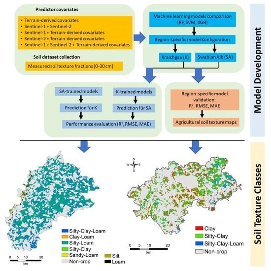
2. Materials and Methods

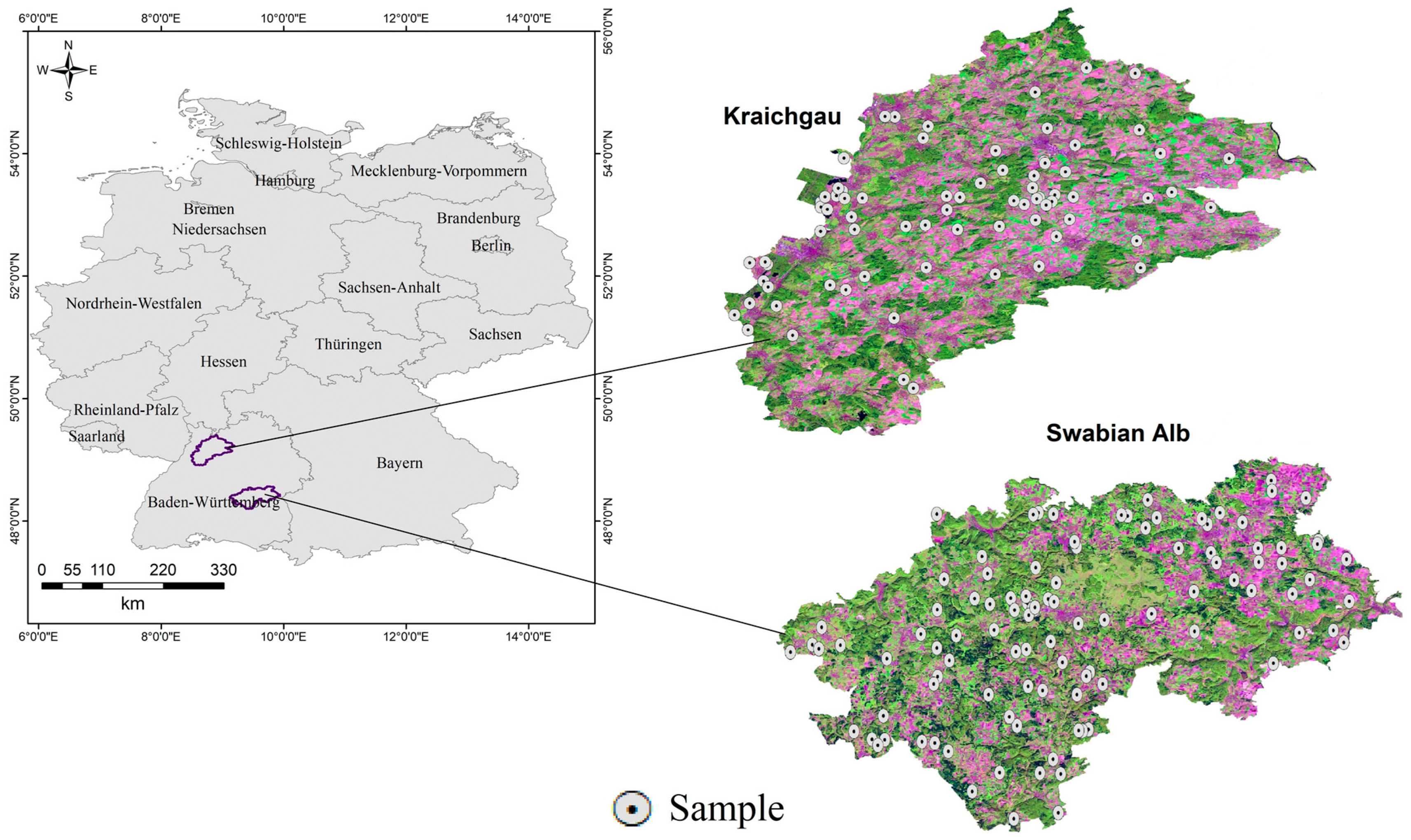
2.1. Study Areas and Soil Sampling

The study sites were two agroecological regions, Kraichgau (K) and Swabian Alb (SA), in Southwest Germany (Figure 1). Each study site covered an area of approximately 1600 km2 centered on 49°04′N, 8°48′E and 48°25′N, 9°29′E, respectively. The Kraichgau region is located at 100–400 m a.s.l. with soils formed mainly from loess. It is a part of the Neckar River watershed with an annual mean temperature of more than 9 °C and mean annual precipitation of 720 to 830 mm. The Swabian Alb is a low mountain plateau in Southwest Germany located at an altitude of 500–850 m a.s.l. with an annual average temperature of 6–7 °C and mean annual precipitation between 800 and 1000 mm. Its soils developed mainly on Jurassic limestone and have a high clay content due to strong decalcification and weathering. Further details can be found in Fischer et al. [37], Ingwersen et al. [38], and Ali et al. [39]. Bulk soil samples were taken (0–30 cm) from agricultural fields during field campaigns via a probability-based sampling design (e.g., simple randomized and regular grid sampling) across the two regions [40]. A sample size of 75 (for K) and 105 (for SA) of these archived soils were analyzed for soil particle size fractions (e.g., sand, silt, and clay) based on German classification (2000–63 µm of sand, 63–2 µm of silt, and < 2 µm of clay) [41] following the pipette method [42]. Briefly, 20 g of < 2 mm soil samples were first checked for CaCO3 by adding a few drops of 10% HCl. Soil organic carbon was removed by adding 6 mL of 30% hydrogen peroxide (H2O2) solution and was heated to 80 °C. Then, samples were rinsed and centrifuged. Sand was first separated out using wet sieving with a 63 µm sieve size. The remaining silt and clay contents were then determined by measuring the rate of settling of these two separates from the suspension in water. The time required for silt and clay to settle was calculated using Stokes law. Next, sand, silt, and clay contents were converted into the World Reference Base particle size classification system (2000–50 µm of sand, 50–2 µm of silt, and < 2 µm of clay) [43] using the R package “soil texture” [44].

2.2. Remote Sensing Data (RS)

In this study, RS data from two freely available missions operated by the European Space Agency (ESA), S1 and S2, were used for estimating soil texture in the 0–30 cm depth [45,46]. S1 allows full polarimetric imaging, i.e., horizontal transmit and receive (HH), horizontal transmit and vertical receive (HV), vertical transmit and horizontal receive (VH), and vertical transmit and receive (VV), at a resolution of 5–20 m every 12 days. This study used dual-polarized SAR level-1 ground range detected products (VH, VV) in ‘IW’ mode as the original data was at a resolution of 10 m. Multiploidization SAR allows a better understanding of soil surface properties compared only to the backscatter coefficients of a single polarization. Several preprocessing algorithms, including radiometric and geometric correction, speckle filtering, and thermal noise removal, were applied to each SAR image to draw out the backscatter coefficient at any polarization mode. These allow reducing error propagation in the following processes and analyses. S2 is a space-borne multispectral spectral imager with a five-day revisit time, which started its mission first in June 2015 as part of the “Copernicus” program. The S2 image comprises 13 spectral bands in the optical domain (VNIR/SWIR) at spatial resolutions of 10, 20, and 60 m. After excluding B1 (Coastal Aerosol), the remaining 11 bands (i.e., B2 (490 nm), B3 (560 nm), B4 (665 nm), B5 (705 nm), B6 (740 nm), B7 (783 nm), B8 (842 nm), B9 (945 nm), B10 (1375 nm), B11 (1610 nm), and B12 (2190 nm)) were extracted for further use (Table 1). The present study acquired the median of S1 and cloud-free multitemporal S2 images for three periods of time, including April–May (T1), August–September (T2) and October–November (T3) 2015-2016 from Google Earth Engine [47].

2.3. Terrain-Derived Covariates (TDC)

In this study, a free digital elevation model (DEM) from the Shuttle Radar Topography Mission (SRTM) [48] was used for deriving terrain-derived covariates (TDC). There are several TDC that can be extracted from DEMs which are directly or indirectly related to soil properties. According to this, the 10 terrain attributes involved in controlling the spatial distribution of texture fractions were derived from a preprocessed DEM with a 30 m resolution using SAGA GIS software [49] to explain the spatial variability of soil texture fractions (i.e., clay, silt, and sand). The included TDC were related to local-scale terrain morphology (e.g., elevation and aspect), hydrological characteristics (e.g., length–slope factor, topographic wetness index), and landscape-scale morphometry (Table 1).

2.4. Machine Learning Models

2.4.1. Random Forest (RF)

Initially introduced by Breiman [50], RF is an ensemble learning algorithm used for regression and classification tasks. RF is an adjusted version of bagged decision trees made of large decorrelated trees that require a few tuning parameters [51]. RF is composed of a reimplementation of the classification and regression tree (CART) model based on the bootstrap sampling. Bootstrapping is a resampling method that generates several datasets equal to the size of the original data [52]. In bootstrapping, some records will be selected multiple times due to the allowance of sampling with replacement, whereas others will not be selected. Unselected records, known as out-of-bag errors, assess model performance. Within the RF algorithm, the mtry parameter was tuned, which denotes the number of explanatory variables for splitting at each tree node.

2.4.2. Support Vector Regression (SVR)

Introduced by Cortes and Vapnik [53], support vector machines (SVMs) are learning models frequently used for distribution estimation, regression, and classification tasks. SVMs transform original independent variables into a higher or infinite dimensional feature space using nonlinear techniques. They aim to create a better separation [54]. The regression task is called support vector regression (SVR); nevertheless, the goal of the classification and regression problem is to minimize error. The kernels used were linear (LN), polynomial (PL), radial basis function (RBF), and sigmoid (SIG); each requires specific parameters, and the proper selection and parameterization of these kernels control the accuracy of the SVR [53]. Tuning parameters were C, known as the penalty factor, to avoid overfitting and to regulate the trade-off between the margins and training errors [55]. The degree of nonlinearity was controlled by the kernel width or gamma (γ) parameter.

2.4.3. Extreme Gradient Boosting (XGB)

XGB is a scalable tree boosting method known for its performance and speed [56]. XGB constructs several consequent decision trees based on the criterion of residuals of the previous tree model or of prediction errors; thus, the algorithm principally marks the samples with higher uncertainty, and, lastly, the generated results are added to calculate the final output [57]. XGB has numerous tuning parameters that make the model complicated, most of which are similar to other tree-based models, plus some hyperparameters intended to lessen the risk of overfitting, reducing prediction variability, and thus increasing the accuracy [51]. Tuning parameters in XGB [51] used were: nrounds, to determine the maximum number of iterations; max_depth, to control the depth of the tree; eta, to control the learning rate for capturing the patterns in data; gamma, to control regularization to prevent overfitting; colsample_bytree, the number of variables provided for a tree; min_child_weight, the tree splitting stops when the leaf node has a minimum sum of instance weight lower than min_child_weight in the classification task; and the last tuning parameter is subsample which controls the number of observations provided for a tree.

2.5. Model Evaluation

Identifying the optimum parameters and model performance was conducted using a 10-fold cross-validation approach to assess the performance of the calibrated model on new data. Ten-fold cross-validation is a resampling process in which all data are randomly divided into ten equal folds; at each run, one-fold is set out for validation, and the remaining k − 1 folds are used for calibration [58]. Then, the final accuracy is computed from the average accuracy of all folds. Three performance indicators were used to evaluate the prediction accuracy of models: R2, root-mean-square error (RMSE), and the mean absolute error (MAE) of cross-validation. All machine learning modeling was done in R Studio with the “Caret” package [59].

3. Results

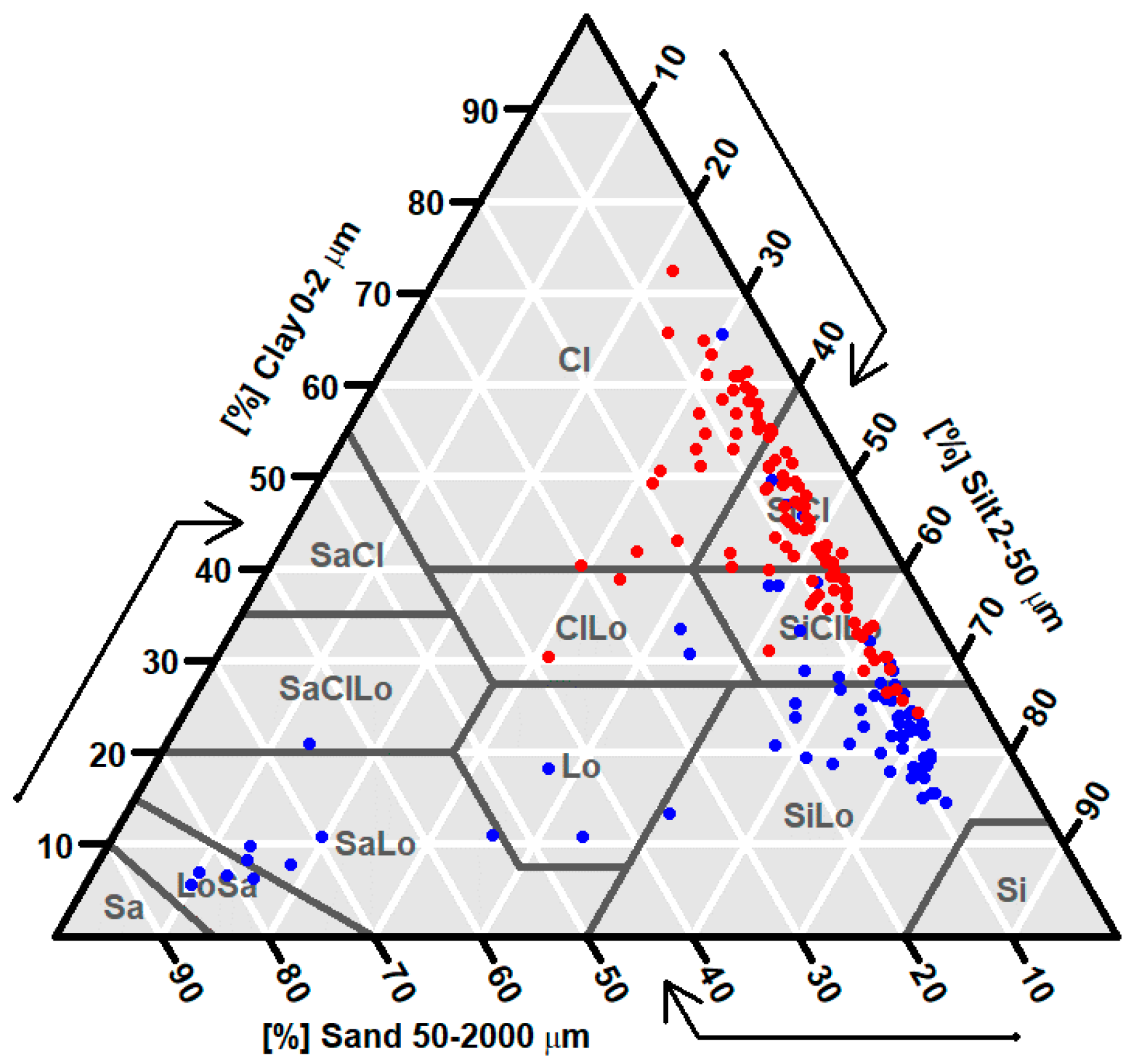
3.1. Summary Statistics of Soil Texture Data

The descriptive characteristics of the measured soil texture fractions for each study region are shown in Table 2. In the K region, the silt contents were highest, with a mean value of 56.7%, whereas the clay and sand fractions were 23.1% and 20.3%, respectively. The sand content varied from 3.4 to 84.3% with a standard deviation (SD) of 22.8%, while the clay and silt contents varied from 10.2 to 76.6% (SD = 18.7%) and 5.6 to 65.4% (SD = 10.2%), respectively. According to the WRB soil texture classes, considering the high silt contents, the soils would typically be classified as silt loam and silty clay loam in the K region. In contrast, the clay and silt sizes dominated in the SA region, representing an average of 46% and 45.2%, respectively, followed by a sand content of 8.8%. Unlike the K region, the silt and clay contents showed the largest variability with SDs of 10.39 and 10.2%, respectively, while the sand contents ranged from 4.1% to 38.4% with an SD of 5.3%. Given that the clay content of the field observation in the entire SA region was over 40%, the soils would typically be classified as clay and silty clay textures. There was a wide range of soil texture classes in the SA region, which included 9 out of the 12 possible texture classes. However, the dominant texture classes across both regions were silt loam (27%), silty clay (25%), silty clay loam (22%), and clay (17%). The remaining 10 percent of measured samples represented other soil texture types (Figure 2).
The variability of the texture within the two regions was mainly due to both intrinsic (e.g., parent material, climate, mineralogy, and soil-forming processes) and extrinsic (e.g., land use type and management practices) factors [60]. The Rhine Valley typically had sandy soil texture classes surrounded by soils with higher silt and clay contents in the K region. Farming with different crop types demands differing plowing practices, resulting in variability in texture fractions within the two regions. Topography, erosion, and deposition also may result in high variability in texture fractions [61].

3.2. Model Performance

Three different ML models were used for predicting soil texture fractions and were evaluated using a 10-fold cross-validation strategy. The model accuracy and predictor selections for the SA and K regions are shown in Table 3 and Table 4, respectively. The prediction accuracy varied among different models and selected predictors in terms of the RMSE, R2, and MAE. As shown, the application of TDC and RS data (S1 + S2) alone resulted in the lowest accuracies with some exceptions. In the SA region, the synergic application of all covariates (S1 + S2 + TDC) generally increased model performance. However, an exception was the SVM model where the S2 + TDC predictor selection strategy was most precise for sand predictions, resulting in an RMSE = 3.6%, R2 = 0.42, and MAE = 2.6%. Although the S1 + S2 + TDC predictors yielded an improved accuracy with the XGB model than other predictor selection strategies, the model performance was still significantly lower (RMSE = 4.4; R2 = 0.33) compared to the RF and SVM models for sand prediction. Regardless of the ML model, the S1 + S2 + TDC predictor selection strategy resulted in the best model performance when predicting silt contents. Indeed, again, the SVM model using S1 + S2 + TDC was most accurate, with an RMSE of 7.3% and an R2 of 0.54. For clay estimates, the XGB model was the most accurate, with an RMSE = 6.8% and an R2 = 0.64, using the S1 + S2 + TDC predictors.
Relatively similar trends in the model accuracy of the K region were observed by changing the model input predictors, where the S1 + S2 + TDC predictors increased clay and sand model performance using the SVM and XGB models, respectively. For sand prediction, the XGB model was most robust with S1 + S2 + TDC predictors, yielding an RMSE = 7.5 and an R2 = 0.79. In terms of the clay predictions, the SVM with S1 + S2 + TDC predictors was most accurate, resulting in an RMSE = 6.1 and an R2 = 0.48. For the silt content, XGB showed the highest performance again but with S1 + TDC predictors and RMSE and R2 values of 7.9 and 0.85, respectively.

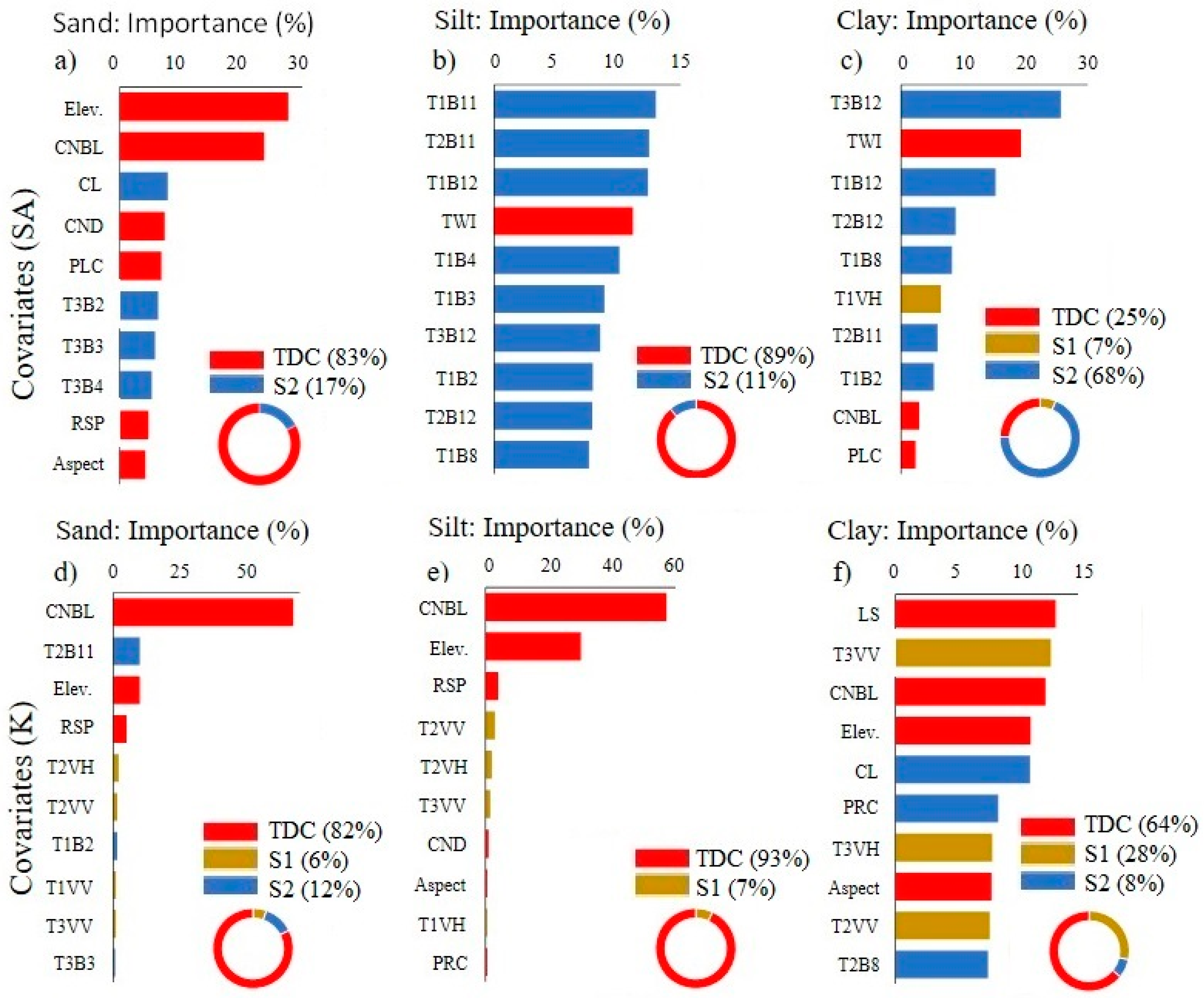
3.3. Variable Importance for Computational Models

Figure 3 gives the relative importance of predictor covariates for the best-fitting ML models used for texture fraction prediction. Only the top 10 predictors for model fitting are shown. The relative importance of predictor covariates differed both by region and by model type. The selected predictors were ordered in the selection process by their influence or by the order in which they were contributed. S2 and TDC explained 17.5% and 82.5% of the sand variation in the SA region, respectively. The elev. (27.7%) and CNBL (23.7%) were the most strongly relevant covariates in fitting the learning models, followed by less relevant predictors such as CI, CND, PLC, B2, B3, and B4. S2 covariates accounted for 88.8% of the total variation for predicting the silt content, followed by TDC with a relative importance of only 11%. The S2 features in SWIR, such as B11 and B12, were the most essential variables in model fitting. The TWI was the only terrain-derived covariate contributing to model fitting, accounting for only 11% of silt variation. The best-fit models for clay and silt contents had relatively similar selected variables. As shown in Figure 3, S1, S2, and TDC accounted for 6.5%, 69%, and 24% of clay variation. The model identified mainly B12 (41%) and TWI (19%) as the most relevant covariates for clay predictions.
In the K region, the contributions of S1, S2, and TDC in describing sand variation were 5%, 12%, and 82%, respectively. The CNBL had the highest importance, accounting for 67% of the total sand variation. Likewise, the CNBL (57%) and elev. (30%) were the most important covariates for silt prediction, followed by the RSP, VV, and VH. Comparably, TDC accounted for 64% of the clay variation, while S1 and S2 explained 28 and 8% of clay variation, respectively. The results showed that the LS (13%), VV (13%), CNBL (12%), Elev. (11%), and CL (11%) were the most critical covariates describing clay variation.

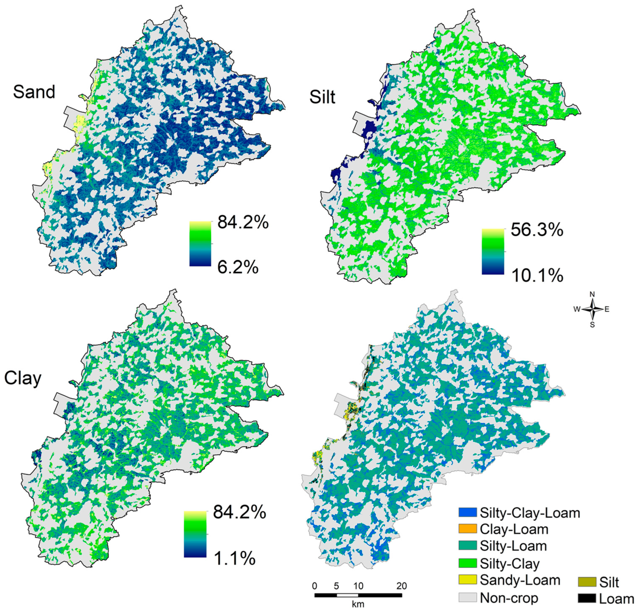
3.4. Mapping of Soil Textural Classes within the Training Region

The best model, described in Section 3.2, was applied to create the spatial prediction map of texture fractions and, later, the texture classes for both training regions separately. Figure 4 shows the spatial prediction of texture fractions and texture maps in the SA region. The visual inspection of the continuous maps displayed a relatively homogenous distribution of the sand content in the SA region, ranging mainly from 5.8% to 25.8%. For the silt content, a mosaic pattern with three different classes was obtained: silt content < 30%, between 30 and 60%, and >60%. Clay contents between 30 and 50% were dominating, covering mainly the center and partially covering the southwestern region. Interestingly, the areas with a higher clay content corresponded with relatively high altitudes. The SA region was classified mostly into three soil texture classes, including silty clay, clay and silty clay loam, corroborating the field observations. The silty clay texture was dominant, covering roughly 70% of the entire region. The silty clay loam texture dominated mainly in the eastern areas of the study region. The clay texture class was observed mainly in the central part of the region.
In the K region, the soils in the western regions represented high sand contents >70%. While the silt contents between 30 and 60% were dominant in the SA, there was a higher silt content (>60%) in the K region. The clay content could be split into three different classes as follows: <30%, 30–50%, and >50%. Clay contents of less than 30% dominated the region. Silt loam was the dominant texture class, covering roughly 67% of the entire area. A small area at the western edge of the study region in the Rhine Valley represented a heterogenous textures with relatively high sand contents, including sandy loam, loam and clay loam texture classes (Figure 5).

3.5. Spatial Transferability of Best-Fitted Models Outside the Training Region

To test the model transferability, the best-fit models using RS data and the terrain-derived predictors in each training region (shown in Section 3.2) were further applied separately to predict the texture fractions for croplands in the other region with the prediction accuracies in Table 5. The soil-texture-fraction prediction accuracy for the K region dramatically decreased when the best-fit SA region models were used. Generally, the performance of all the best fit models was poor in predicting texture fractions in a new geographic region. For sand prediction in the K region, the RMSE increased to 25.2%, which was six times higher than in the transferred model (SA_Sand_SVM_S2 + TDC). The accuracy also declined for silt and clay prediction in K with an increased RMSE of 24.3% and 19.8% compared to those in the original models, i.e., SA_Silt_SVM_S1 + S2 + TDC and SA_Clay_XGB_S1 + S2 + TDC, respectively. Likewise, the R2 decreased, and the MAE increased. In the SA region, in sand prediction with the K_Sand_XGB_S1 + S2 + TDC model, the RMSE value increased to 6.1%, and the R2 declined to 0.003. For silt and clay contents, similar trends in the RMSE were observed again with an increase to 19.6 and 10.2, respectively. Thus, the models performed best for both regions when the calibration points were located within the respective application area (within the training region; Section 3.4).

4. Discussion

4.1. Variable Importance for ML Models

Our study evaluated the potential use of TDC and RS data as covariates in five combinations (S1 + S2, TDC, S1 + TDC, S2 + TDC, and S1 + S2 + TDC) to predict soil texture fractions using three different ML models (RF, the SVM, and XGB) across two contrasting agroecological regions (SA and K). Our results indicated that, due to the environmental and soil differences as well as the RS data quality, the performance of the trained models was different in predicting texture fractions within the individual regions (Table 3 and Table 4), which was consistent with the results of previous studies dealing with estimating soil properties using RS data [31,32,36,62]. Importantly, the addition of TDC to RS data (i.e., S1 + S2 + TDC) outperformed the use of any of TDC or RS data alone. Apart from the specific ML model type, the prediction accuracies in the combined mode of RS and TDC for sand, silt, and clay contents varied with an R2 ranging from 0.49 to 0.64, with roughly 20 and 22% improvements compared to the application of TDC or RS data alone, respectively. The results corroborated previous studies focusing on the combined use of RS data in estimated soil carbon as well as texture fractions [28,62,63]. However, it should be highlighted that the sensitivity of optical RS to the atmospheric effects (clouds, particles, and gas molecules) and soil surface conditions affecting spectral reflection might be the leading causes of their lower accuracies than those of combined modes. Furthermore, the spectral reflection from the soil is primarily affected by surface crop residues after harvesting or plowing as well as the soil moisture condition [3,15,28,64,65]. Thus, a diverse range of estimation accuracies has been reported in the literature depending on both climate and farming practices.
Furthermore, our results indicated the significant contribution of SWIR bands (B11 and B12) in the optical domain and TDC data (CNBL, Elev., TWI, and LS) in model training for silt and clay prediction. However, variable selection was dramatically affected by the training regions. While RS data had a significant role in model training in the SA region, TDC contributed markedly to predicting silt and clay contents in the K region. Similar to our findings are those reported by Meyer et al. [66], Marzahn and Meyer [24], and Taghizadeh-Mehrjardi et al. [62] who found TDC to be the most important predictors in soil texture fraction prediction. Bousbih et al. [28] and Gholizadeh et al. [29] revealed that the SWIR bands of S2 (B11 and B12) had a considerable potential to estimate clay contents, which also corroborates the findings in the current study. It was concluded that the Sentinel SWIR bands assigned to soil minerals provide a spectral predictor for different mineral constituents, including texture fractions [67]. In general, the contribution of S1 data was relatively lower than S2 and TDC in predicting texture fractions, ranging from 0 to 28% depending on the best-performing models and representing the relatively moderate importance of VV and VH polarizations in model fitting. Several studies have already reported that VH and VV polarizations are sensitive to soil moisture dynamics and surface roughness and that they mainly contribute to describing different soil properties [68]. In contrast, Matti et al. [69] reported that the HH polarization has a higher sensitivity to soil properties than VV and VH.
Despite the limited studies focusing on radar data in this context, it seems to improve the accuracy in estimating soil surface properties, specifically when combined with either optical or TDC data. It can collect spectral data through the clouds and give other signals from the surface soil due to its longer wavelength [23,28]. Furthermore, backscattered radar signals are assigned to the soil moisture content as a robust representative of soil moisture conditions. Soil with a higher clay content tends to retain moisture longer and to dry slowly. Thus, the estimation of soil textures, specifically clay content, could improve when backscattered radar signals are applied [26,28]. In our study, the sensitivity of SAR data was observed by other authors when quantifying different soil properties. Marzahn and Meyer [24] estimated the soil texture precisely in sandy loam soil at the field scale with a mean RMSE of 2.42 (Mass-%) using SAR data at 1.3 GHz linked to geostatistics. An RMSE of 1.2% for the clay content was also obtained by Zribi et al. [26]. The best-fit models in the current study for soil texture had an RMSE of 5.1 and 7.2% in the SA and K regions, respectively. The higher RMSE in our study might be due to the large-scale sample collection across the two regions on farms, representing different surface conditions in terms of soil moisture, retained crop residues, and partial vegetation cover, which further affected the quality of the acquired RS data.

4.2. Accuracy Assessment of ML Models

Usually, ML models outperform simple models and increase the predictive power of models in understanding the specification of the soil horizon in a soil profile [70], explaining soil variability [31], and helping to understand the causes of soil variability [35]. However, ML model robustness demands more data and meaningful predictors to avoid overfitting or misleading results and to improve the interpretability of the model and, consequently, our understanding of soil. Thus, it is worth adopting more predictor covariates from multiple data sources, including categorical maps, climatic data, terrain attributes, and remote sensing data. In the current study, texture fractions were predicted with the best model, with R2 values of 0.49–0.64 and 0.48–0.85 for the SA and K regions, respectively (Table 3 and Table 4). In comparison, using optical S2 data resulted in clay fraction predictions in the model, with R2 values of 0.39–0.42 and R2 < 0.22 for silt and sand using the partial least squares regression [21]. Bousbih et al. [28], in contrast, using derived soil moisture contents from S1 combined with S2, provided improved estimates of clay contents with an overall accuracy of R2 = 0.55, even in areas covered by vegetation and in areas under different climatic conditions. Moreover, Castaldi et al. [71] demonstrated that the prediction of clay contents was more accurate when the soil moisture content increased using clay indices in the optical domain. More robustly, Rosero-Vlasova et al. [72] reported R2 values of 0.54 and 0.7 in predicting clay contents using Landsat and S2 data, respectively.
Generally speaking, the range of the prediction accuracies for the best-performing models within any region (Figure 4 and Figure 5) indicated a comparable performance to those studies previously cited. Additionally, in the same study regions, lab-based proximal sensing (midinfrared spectroscopy) resulted in an RMSE of 2.7, 4.6, and 3.1% for sand, silt, and clay contents, respectively [73]. But the transferability of the region-specific model to the other region strongly decreased the predictive performance. The possible reason might be attributed to the environmental, climatic, terrain, and soil differences between the two study regions, resulting in different variable contributions in model developments (Figure 3). Thus, a region-specific trained model may not encompass a new, unknown area’s intrinsic and extrinsic spatial heterogeneity. Therefore, the trained models within each training region could not describe the soil texture fraction variability outside their training region. Our findings were in line with the findings of the other researchers [74,75,76] who indicated that ML models have a low accuracy in spatial extrapolations due to the complexity of the spatial variation in soil and the difficulty of matching soil-forming factors exactly between two areas. It is worth noting that the similarity of the environmental covariates between two regions (i.e., soils of two areas are mainly controlled by similar soil-forming factors) plays an important role in achieving the transferable ML models for predicting soil properties and soil classes. Nevertheless, splitting the regions into finer geographic scales, such as the slope-aspect class, may improve the predictive results of transferability [77,78]. An alternative option is the use of more advanced ML models, such as semi-supervised learning which is a branch of ML that benefits from both supervised and unsupervised learning, which can be more effective in the spatial extrapolation of soils [79,80].

5. Conclusions

This paper examined the capability of satellite imagery (S1 and S2) and terrain-derived covariates (TDC) in estimating soil texture fractions and evaluated the spatial transferability of three machine learning models. Due to the complexity of the influential factors of soil properties (e.g., intrinsic and extrinsic) across the study regions, model performance was not consistent, even for different models in the same area. Taking sand prediction as an example, the SVM performed the best in the SA, while XGB was most accurate in the K region. Thus, the soil texture was mapped in each training region based on the most accurate model for each texture fraction. Regardless of the region or model, RS (S1 and S2) data alone did not have an adequate capability in estimating the texture fractions in the training regions. Due to the spectral response of soil, which is controlled by several factors (such as soil moisture, organic matter, surface roughness, atmospheric effects, structural effects, soil management, and vegetative coverage) and the technical constraints on the acquisition of RS data (specifically S2), using RS data alone to estimate soil texture fractions is still challenging. However, the model derived from combined data (RS and TDC) outperformed the models developed according to their sole application. This confirmed the dependency of texture fractions on both terrain-derived covariates and intrinsic soil attributes. While the ML models improved the texture fraction accuracy with RS data, the best-performing models in each training region led to poor performances in predicting texture fractions when transferred to the other region where the models were not trained. To increase the prediction accuracy, further studies should involve other sources of covariates such as climatic variables and multipolarization L-band SAR data in the microwave domain. To conclude, first, our results indicated that ML models are highly acknowledged because they enhance the prediction accuracy of soil while reducing the margin of error. Nonetheless, due to the heterogeneity of landscapes and influential factors, it is necessary to combine RS data with TDC for soil texture mapping at the regional scale. Second, region-specific calibrated models cannot be applied to other regions without a considerable loss of prediction accuracy. Thus, further research to evaluate the added value of Sentinel imagery, to better analyze the spatial transferability of the machine learning models, and to reveal the unclear problem is highly recommended.

Author Contributions

Conceptualization, R.M. and H.S.-M.; methodology, R.M., H.S.-M. and M.S.D.; software, H.S.-M. and R.T.-M.; validation, H.S.-M.; formal analysis, R.M.; investigation, R.M. and M.S.D.; resources, R.M.; data curation, R.M.; writing—original draft preparation, R.M.; writing—review and editing, R.M., M.S.D., H.S.-M. and R.T.-M.; visualization, R.M., H.S.-M. and R.T.-M.; supervision, R.M.; funding acquisition, R.M. All authors have read and agreed to the published version of the manuscript.

Funding

This research was financed by the Alexander von Humboldt Foundation.

Data Availability Statement

The data presented in this study are available on request from the corresponding author. The data are not publicly available due to privacy restrictions.

Acknowledgments

The authors thank Torsten Müller for hosting and supporting R.M. at the Institute of Crop Science, University of Hohenheim, and for his valuable comments and suggestions. We would like to thank David Eugene Stoltzfus Lapp Jost for editing the manuscript.

Conflicts of Interest

The authors declare that they have no known competing financial interests or personal relationships that could have appeared to influence the work reported in this paper.

References

  1. Hartemink, A.E.; McBratney, A. A Soil Science Renaissance. Geoderma 2008, 148, 123–129. [Google Scholar] [CrossRef]
  2. Dharumarajan, S.; Hegde, R. Digital Mapping of Soil Texture Classes Using Random Forest Classification Algorithm. Soil Use Manag. 2022, 38, 135–149. [Google Scholar] [CrossRef]
  3. Castaldi, F.; Palombo, A.; Santini, F.; Pascucci, S.; Pignatti, S.; Casa, R. Evaluation of the Potential of the Current and Forthcoming Multispectral and Hyperspectral Imagers to Estimate Soil Texture and Organic Carbon. Remote Sens. Environ. 2016, 179, 54–65. [Google Scholar] [CrossRef]
  4. Dharumarajan, S.; Hegde, R.; Lalitha, M.; Kalaiselvi, B.; Singh, S.K. Pedotransfer Functions for Predicting Soil Hydraulic Properties in Semi-Arid Regions of Karnataka Plateau, India. Curr. Sci. 2019, 116, 1237. [Google Scholar] [CrossRef]
  5. Thompson, J.A.; Roecker, S.; Grunwald, S.; Owens, P.R. Digital soil mapping. In Hydropedology; Elsevier: Amsterdam, The Netherlands, 2012; pp. 665–709. ISBN 978-0-12-386941-8. [Google Scholar]
  6. Pachepsky, Y.; Rawls, W.J. Development of Pedotransfer Functions in Soil Hydrology, 1st ed.; Elsevier: Oxford, UK, 2004; ISBN 9780080530369. [Google Scholar]
  7. Bockheim, J.G.; Hartemink, A.E. Distribution and Classification of Soils with Clay-Enriched Horizons in the USA. Geoderma 2013, 209–210, 153–160. [Google Scholar] [CrossRef]
  8. Arrouays, D.; Grundy, M.G.; Hartemink, A.E.; Hempel, J.W.; Heuvelink, G.B.M.; Hong, S.Y.; Lagacherie, P.; Lelyk, G.; McBratney, A.B.; McKenzie, N.J.; et al. Chapter three—GlobalSoilMap: Toward a fine-resolution global grid of soil properties. In Advances in Agronomy; Sparks, D.L., Ed.; Academic Press: Cambridge, MA, USA, 2014; Volume 125, pp. 93–134. [Google Scholar]
  9. Niang, M.A.; Nolin, M.C.; Jégo, G.; Perron, I. Digital Mapping of Soil Texture Using RADARSAT-2 Polarimetric Synthetic Aperture Radar Data. Soil Sci. Soc. Am. J. 2014, 78, 673–684. [Google Scholar] [CrossRef]
  10. Forkuor, G.; Hounkpatin, O.K.L.; Welp, G.; Thiel, M. High Resolution Mapping of Soil Properties Using Remote Sensing Variables in South-Western Burkina Faso: A Comparison of Machine Learning and Multiple Linear Regression Models. PLoS ONE 2017, 12, e0170478. [Google Scholar] [CrossRef] [Green Version]
  11. Mulla, D.J.; Beatty, M.; Sekely, A.C. Evaluation of remote sensing and targeted soil sampling for variable rate application of lime. In Proceedings of the 5th International Conference on Precision Agriculture, Bloomington, MN, USA, 16–19 July 2000; Robert, P.C., Rust, R.H., Larson, W.E., Eds.; ASA-CSSA-SSSA. American Society of Agronomy: Madison, WI, USA, 2001. [Google Scholar]
  12. Manchanda, M.L.; Kudrat, M.; Tiwari, A.K. Soil Survey and Mapping Using Remote Sensing. Trop. Ecol. 2002, 43, 61–74. [Google Scholar]
  13. Mulder, V.L.; de Bruin, S.; Schaepman, M.E.; Mayr, T.R. The Use of Remote Sensing in Soil and Terrain Mapping—A Review. Geoderma 2011, 162, 1–19. [Google Scholar] [CrossRef]
  14. Malone, B.P.; Jha, S.K.; Minasny, B.; McBratney, A.B. Comparing Regression-Based Digital Soil Mapping and Multiple-Point Geostatistics for the Spatial Extrapolation of Soil Data. Geoderma 2016, 262, 243–253. [Google Scholar] [CrossRef]
  15. Gomez, C.; Adeline, K.; Bacha, S.; Driessen, B.; Gorretta, N.; Lagacherie, P.; Roger, J.M.; Briottet, X. Sensitivity of Clay Content Prediction to Spectral Configuration of VNIR/SWIR Imaging Data, from Multispectral to Hyperspectral Scenarios. Remote Sens. Environ. 2018, 204, 18–30. [Google Scholar] [CrossRef]
  16. Chabrillat, S.; Ben-Dor, E.; Cierniewski, J.; Gomez, C.; Schmid, T.; van Wesemael, B. Imaging Spectroscopy for Soil Mapping and Monitoring. Surv. Geophys. 2019, 40, 361–399. [Google Scholar] [CrossRef] [Green Version]
  17. Dematte, J.A.M.; Fiorio, P.R.; Ben-Dor, E. Estimation of Soil Properties by Orbital and Laboratory Reflectance Means and Its Relation with Soil Classification. Open Remote Sens. J. 2009, 2, 12–23. [Google Scholar] [CrossRef]
  18. Castaldi, F.; Casa, R.; Castrignanò, A.; Pascucci, S.; Palombo, A.; Pignatti, S. Estimation of Soil Properties at the Field Scale from Satellite Data: A Comparison between Spatial and Non-Spatial Techniques: Estimation of Soil Properties from Satellite Data. Eur. J. Soil Sci. 2014, 65, 842–851. [Google Scholar] [CrossRef]
  19. Wu, J.; Li, Z.; Gao, Z.; Wang, B.; Bai, L.; Sun, B.; Li, C.; Ding, X. Degraded Land Detection by Soil Particle Composition Derived from Multispectral Remote Sensing Data in the Otindag Sandy Lands of China. Geoderma 2015, 241–242, 97–106. [Google Scholar] [CrossRef]
  20. Shabou, M.; Mougenot, B.; Chabaane, Z.; Walter, C.; Boulet, G.; Aissa, N.; Zribi, M. Soil Clay Content Mapping Using a Time Series of Landsat TM Data in Semi-Arid Lands. Remote Sens. 2015, 7, 6059–6078. [Google Scholar] [CrossRef] [Green Version]
  21. Vaudour, E.; Gomez, C.; Fouad, Y.; Lagacherie, P. Sentinel-2 Image Capacities to Predict Common Topsoil Properties of Temperate and Mediterranean Agroecosystems. Remote Sens. Environ. 2019, 223, 21–33. [Google Scholar] [CrossRef]
  22. Moreira, A.; Prats-Iraola, P.; Younis, M.; Krieger, G.; Hajnsek, I.; Papathanassiou, K.P. A Tutorial on Synthetic Aperture Radar. IEEE Geosci. Remote Sens. Mag. 2013, 1, 6–43. [Google Scholar] [CrossRef] [Green Version]
  23. Ulaby, F.T.; Long, D.G. Microwave Radar and Radiometric Remote Sensing; The University of Michigan Press: Ann Arbor, MI, USA, 2014; ISBN 978-0-472-11935-6. [Google Scholar]
  24. Marzahn, P.; Meyer, S. Utilization of Multi-Temporal Microwave Remote Sensing Data within a Geostatistical Regionalization Approach for the Derivation of Soil Texture. Remote Sens. 2020, 12, 2660. [Google Scholar] [CrossRef]
  25. Baghdadi, N.; Zribi, M.; Loumagne, C.; Ansart, P.; Anguela, T.P. Analysis of TerraSAR-X Data and Their Sensitivity to Soil Surface Parameters over Bare Agricultural Fields. Remote Sens. Environ. 2008, 112, 4370–4379. [Google Scholar] [CrossRef] [Green Version]
  26. Zribi, M.; Kotti, F.; Lili-Chabaane, Z.; Baghdadi, N.; Ben Issa, N.; Amri, R.; Amri, B.; Chehbouni, A. Soil Texture Estimation Over a Semiarid Area Using TerraSAR-X Radar Data. IEEE Geosci. Remote Sens. Lett. 2012, 9, 353–357. [Google Scholar] [CrossRef]
  27. Gorrab, A.; Zribi, M.; Baghdadi, N.; Mougenot, B.; Fanise, P.; Chabaane, Z. Retrieval of Both Soil Moisture and Texture Using TerraSAR-X Images. Remote Sens. 2015, 7, 10098–10116. [Google Scholar] [CrossRef] [Green Version]
  28. Bousbih, S.; Zribi, M.; Pelletier, C.; Gorrab, A.; Lili-Chabaane, Z.; Baghdadi, N.; Ben Aissa, N.; Mougenot, B. Soil Texture Estimation Using Radar and Optical Data from Sentinel-1 and Sentinel-2. Remote Sens. 2019, 11, 1520. [Google Scholar] [CrossRef] [Green Version]
  29. Gholizadeh, A.; Žižala, D.; Saberioon, M.; Borůvka, L. Soil Organic Carbon and Texture Retrieving and Mapping Using Proximal, Airborne and Sentinel-2 Spectral Imaging. Remote Sens. Environ. 2018, 218, 89–103. [Google Scholar] [CrossRef]
  30. Gomez, C.; Dharumarajan, S.; Féret, J.-B.; Lagacherie, P.; Ruiz, L.; Sekhar, M. Use of Sentinel-2 Time-Series Images for Classification and Uncertainty Analysis of Inherent Biophysical Property: Case of Soil Texture Mapping. Remote Sens. 2019, 11, 565. [Google Scholar] [CrossRef] [Green Version]
  31. Brungard, C.W.; Boettinger, J.L.; Duniway, M.C.; Wills, S.A.; Edwards, T.C. Machine Learning for Predicting Soil Classes in Three Semi-Arid Landscapes. Geoderma 2015, 239–240, 68–83. [Google Scholar] [CrossRef] [Green Version]
  32. Heung, B.; Ho, H.C.; Zhang, J.; Knudby, A.; Bulmer, C.E.; Schmidt, M.G. An Overview and Comparison of Machine-Learning Techniques for Classification Purposes in Digital Soil Mapping. Geoderma 2016, 265, 62–77. [Google Scholar] [CrossRef]
  33. Khaledian, Y.; Miller, B.A. Selecting Appropriate Machine Learning Methods for Digital Soil Mapping. Appl. Math. Model. 2020, 81, 401–418. [Google Scholar] [CrossRef]
  34. Wadoux, A.M.J.-C.; Minasny, B.; McBratney, A.B. Machine Learning for Digital Soil Mapping: Applications, Challenges and Suggested Solutions. Earth-Sci. Rev. 2020, 210, 103359. [Google Scholar] [CrossRef]
  35. Ma, Y.; Minasny, B.; Malone, B.P.; Mcbratney, A.B. Pedology and Digital Soil Mapping (DSM). Eur. J. Soil Sci. 2019, 70, 216–235. [Google Scholar] [CrossRef]
  36. Biney, J.K.M.; Vašát, R.; Bell, S.M.; Kebonye, N.M.; Klement, A.; John, K.; Borůvka, L. Prediction of Topsoil Organic Carbon Content with Sentinel-2 Imagery and Spectroscopic Measurements under Different Conditions Using an Ensemble Model Approach with Multiple Pre-Treatment Combinations. Soil. Till. Res. 2022, 220, 105379. [Google Scholar] [CrossRef]
  37. Fischer, M.; Bossdorf, O.; Gockel, S.; Hänsel, F.; Hemp, A.; Hessenmöller, D.; Korte, G.; Nieschulze, J.; Pfeiffer, S.; Prati, D.; et al. Implementing Large-Scale and Long-Term Functional Biodiversity Research: The Biodiversity Exploratories. Basic Appl. Ecol. 2010, 11, 473–485. [Google Scholar] [CrossRef]
  38. Ingwersen, J.; Steffens, K.; Högy, P.; Warrach-Sagi, K.; Zhunusbayeva, D.; Poltoradnev, M.; Gäbler, R.; Wizemann, H.-D.; Fangmeier, A.; Wulfmeyer, V.; et al. Comparison of Noah Simulations with Eddy Covariance and Soil Water Measurements at a Winter Wheat Stand. Agric. For. Meteorol. 2011, 151, 345–355. [Google Scholar] [CrossRef]
  39. Ali, R.S.; Ingwersen, J.; Demyan, M.S.; Funkuin, Y.N.; Wizemann, H.-D.; Kandeler, E.; Poll, C. Modelling in Situ Activities of Enzymes as a Tool to Explain Seasonal Variation of Soil Respiration from Agro-Ecosystems. Soil Biol. Biochem. 2015, 81, 291–303. [Google Scholar] [CrossRef]
  40. Mirzaeitalarposhti, R.; Demyan, M.S.; Rasche, F.; Cadisch, G.; Müller, T. Mid-Infrared Spectroscopy to Support Regional-Scale Digital Soil Mapping on Selected Croplands of South-West Germany. CATENA 2017, 149, 283–293. [Google Scholar] [CrossRef]
  41. Boden, A.G. Bodenkundliche Kartieranleitung, 5th ed.; Schweizerbart [i. Komm.]: Stuttgart, Germany, 2005; ISBN 978-3-510-95920-4. [Google Scholar]
  42. DIN ISO 11277. In Soil Quality—Determination of Particle Size Distribution in Mineral Soil Material—Method by Sieving and Sedimentation; Beuth: Berlin, Germany, 2009.
  43. WRB. World Reference Base for Soil Resources, 2006: A Framework for International Classification, Correlation, and Communication; Food and Agriculture Organization of the United Nations: Rome, Italy, 2006; ISBN 978-92-5-105511-3. [Google Scholar]
  44. Moeys, J. The Soil Texture Wizard: R Functions for Plotting, Classifying, Transforming and Exploring Soil Texture Data. R package soiltexture Vignette, Version 1.5.1. Available online: https://cran.r-project.org/web/packages/soiltexture/vignettes/soiltexture_vignette.pdf (accessed on 16 February 2022).
  45. Yang, R.-M.; Guo, W.-W. Modelling of Soil Organic Carbon and Bulk Density in Invaded Coastal Wetlands Using Sentinel-1 Imagery. Int. J. Appl. Earth Obs. Geoinf. 2019, 82, 101906. [Google Scholar] [CrossRef]
  46. Zhou, T.; Geng, Y.; Chen, J.; Pan, J.; Haase, D.; Lausch, A. High-Resolution Digital Mapping of Soil Organic Carbon and Soil Total Nitrogen Using DEM Derivatives, Sentinel-1 and Sentinel-2 Data Based on Machine Learning Algorithms. Sci. Total Environ. 2020, 729, 138244. [Google Scholar] [CrossRef]
  47. Gorelick, N.; Hancher, M.; Dixon, M.; Ilyushchenko, S.; Thau, D.; Moore, R. Google Earth Engine: Planetary-Scale Geospatial Analysis for Everyone. Remote Sens. Environ. 2017, 202, 18–27. [Google Scholar] [CrossRef]
  48. Werner, M. Shuttle Radar Topography Mission (SRTM) Mission Overview. Frequenz 2001, 55, 75–79. [Google Scholar] [CrossRef]
  49. Olaya, V.; Conrad, O. Chapter 12 geomorphometry in SAGA. In Developments in Soil Science; Elsevier: Amsterdam, The Netherlands, 2009; Volume 33, pp. 293–308. ISBN 978-0-12-374345-9. [Google Scholar]
  50. Breiman, L. Random Forests. Mach. Learn. 2001, 45, 5–32. [Google Scholar] [CrossRef] [Green Version]
  51. Boehmke, B.; Greenwell, B.M. Hands-On Machine Learning with R; Chapman and Hall/CRC: New York, NY, USA, 2019; ISBN 978-0-367-81637-7. [Google Scholar]
  52. Efron, B.; Tibshirani, R. Bootstrap Methods for Standard Errors, Confidence Intervals, and Other Measures of Statistical Accuracy. Statist. Sci. 1986, 1, 54–75. [Google Scholar] [CrossRef]
  53. Cortes, C.; Vapnik, V. Support-Vector Networks. Mach. Learn. 1995, 20, 273–297. [Google Scholar] [CrossRef]
  54. Moguerza, J.M.; Muñoz, A. Support Vector Machines with Applications. Statist. Sci. 2006, 21, 322–336. [Google Scholar] [CrossRef] [Green Version]
  55. Marjanović, M.; Kovačević, M.; Bajat, B.; Voženílek, V. Landslide Susceptibility Assessment Using SVM Machine Learning Algorithm. Eng. Geol. 2011, 123, 225–234. [Google Scholar] [CrossRef]
  56. Chen, T.; Guestrin, C. XGBoost: A Scalable Tree Boosting System. In Proceedings of the Proceedings of the 22nd ACM SIGKDD International Conference on Knowledge Discovery and Data Mining, ACM; San Francisco, CA, USA, 13 August 2016, pp. 785–794.
  57. Taghizadeh-Mehrjardi, R.; Schmidt, K.; Amirian-Chakan, A.; Rentschler, T.; Zeraatpisheh, M.; Sarmadian, F.; Valavi, R.; Davatgar, N.; Behrens, T.; Scholten, T. Improving the Spatial Prediction of Soil Organic Carbon Content in Two Contrasting Climatic Regions by Stacking Machine Learning Models and Rescanning Covariate Space. Remote Sens. 2020, 12, 1095. [Google Scholar] [CrossRef] [Green Version]
  58. James, G.; Witten, D.; Hastie, T.; Tibshirani, R. An Introduction to Statistical Learning; Springer Texts in Statistics; Springer: New York, NY, USA, 2013; Volume 103, ISBN 978-1-4614-7137-0. [Google Scholar]
  59. Kuhn, M. Building Predictive Models in R Using the Caret Package. J. Stat. Softw. 2008, 28, 1–26. [Google Scholar] [CrossRef] [Green Version]
  60. Wang, Y.; Shao, M.; Liu, Z. Large-Scale Spatial Variability of Dried Soil Layers and Related Factors across the Entire Loess Plateau of China. Geoderma 2010, 159, 99–108. [Google Scholar] [CrossRef]
  61. Amirian-Chakan, A.; Minasny, B.; Taghizadeh-Mehrjardi, R.; Akbarifazli, R.; Darvishpasand, Z.; Khordehbin, S. Some Practical Aspects of Predicting Texture Data in Digital Soil Mapping. Soil Till. Res. 2019, 194, 104289. [Google Scholar] [CrossRef]
  62. Taghizadeh-Mehrjardi, R.; Emadi, M.; Cherati, A.; Heung, B.; Mosavi, A.; Scholten, T. Bio-Inspired Hybridization of Artificial Neural Networks: An Application for Mapping the Spatial Distribution of Soil Texture Fractions. Remote Sens. 2021, 13, 1025. [Google Scholar] [CrossRef]
  63. Shafizadeh-Moghadam, H.; Minaei, F.; Talebi-khiyavi, H.; Xu, T.; Homaee, M. Synergetic Use of Multi-Temporal Sentinel-1, Sentinel-2, NDVI, and Topographic Factors for Estimating Soil Organic Carbon. CATENA 2022, 212, 106077. [Google Scholar] [CrossRef]
  64. Sumfleth, K.; Duttmann, R. Prediction of Soil Property Distribution in Paddy Soil Landscapes Using Terrain Data and Satellite Information as Indicators. Ecol. Indic. 2008, 8, 485–501. [Google Scholar] [CrossRef]
  65. Zhang, Y.; Guo, L.; Chen, Y.; Shi, T.; Luo, M.; Ju, Q.; Zhang, H.; Wang, S. Prediction of Soil Organic Carbon Based on Landsat 8 Monthly NDVI Data for the Jianghan Plain in Hubei Province, China. Remote Sens. 2019, 11, 1683. [Google Scholar] [CrossRef] [Green Version]
  66. Meyer, S.; Blaschek, M.; Duttmann, R.; Ludwig, R. Improved Hydrological Model Parametrization for Climate Change Impact Assessment under Data Scarcity—The Potential of Field Monitoring Techniques and Geostatistics. Sci. Total Environ. 2016, 543, 906–923. [Google Scholar] [CrossRef] [PubMed]
  67. Boettinger, J.L.; Howell, D.W.; Moore, A.C.; Hartemink, A.E.; Kienast-Brown, S. Digital Soil Mapping: Bridging Research, Environmental Application, and Operation, 1st ed.; Springer: Dordrecht, The Netherlands, 2010; ISBN 978-90-481-8862-8. [Google Scholar]
  68. Veloso, A.; Mermoz, S.; Bouvet, A.; Le Toan, T.; Planells, M.; Dejoux, J.-F.; Ceschia, E. Understanding the Temporal Behavior of Crops Using Sentinel-1 and Sentinel-2-like Data for Agricultural Applications. Remote Sens. Environ. 2017, 199, 415–426. [Google Scholar] [CrossRef]
  69. Mattia, F.; Thuy Le, T.; Picard, G.; Posa, F.I.; D’Alessio, A.; Notarnicola, C.; Gatti, A.M.; Rinaldi, M.; Satalino, G.; Pasquariello, G. Multitemporal C-Band Radar Measurements on Wheat Fields. IEEE Trans. Geosci. Remote Sens. 2003, 41, 1551–1560. [Google Scholar] [CrossRef]
  70. Fajardo, M.; McBratney, A.; Whelan, B. Fuzzy Clustering of Vis–NIR Spectra for the Objective Recognition of Soil Morphological Horizons in Soil Profiles. Geoderma 2016, 263, 244–253. [Google Scholar] [CrossRef]
  71. Castaldi, F.; Palombo, A.; Pascucci, S.; Pignatti, S.; Santini, F.; Casa, R. Reducing the Influence of Soil Moisture on the Estimation of Clay from Hyperspectral Data: A Case Study Using Simulated PRISMA Data. Remote Sens. 2015, 7, 15561–15582. [Google Scholar] [CrossRef] [Green Version]
  72. Rosero-Vlasova, O.A.; Vlassova, L.; Pérez-Cabello, F.; Montorio, R.; Nadal-Romero, E. Modeling Soil Organic Matter and Texture from Satellite Data in Areas Affected by Wildfires and Cropland Abandonment in Aragón, Northern Spain. J. Appl. Remote Sens. 2018, 12, 1. [Google Scholar] [CrossRef]
  73. Mirzaeitalarposhti, R.; Demyan, M.S.; Rasche, F.; Poltoradnev, M.; Cadisch, G.; Müller, T. MidDRIFTS-PLSR-Based Quantification of Physico-Chemical Soil Properties across Two Agroecological Zones in Southwest Germany: Generic Independent Validation Surpasses Region Specific Cross-Validation. Nutr. Cycl. Agroecosyst. 2015, 102, 265–283. [Google Scholar] [CrossRef]
  74. Angelini, M.E.; Kempen, B.; Heuvelink, G.B.M.; Temme, A.J.A.M.; Ransom, M.D. Extrapolation of a Structural Equation Model for Digital Soil Mapping. Geoderma 2020, 367, 114226. [Google Scholar] [CrossRef]
  75. Silva, S.H.G.; de Menezes, M.D.; Owens, P.R.; Curi, N. Retrieving Pedologist’s Mental Model from Existing Soil Map and Comparing Data Mining Tools for Refining a Larger Area Map under Similar Environmental Conditions in Southeastern Brazil. Geoderma 2016, 267, 65–77. [Google Scholar] [CrossRef]
  76. Neyestani, M.; Sarmadian, F.; Jafari, A.; Keshavarzi, A.; Sharififar, A. Digital Mapping of Soil Classes Using Spatial Extrapolation with Imbalanced Data. Geoderma Reg. 2021, 26, e00422. [Google Scholar] [CrossRef]
  77. Peng, Y.; Xiong, X.; Adhikari, K.; Knadel, M.; Grunwald, S.; Greve, M.H. Modeling Soil Organic Carbon at Regional Scale by Combining Multi-Spectral Images with Laboratory Spectra. PLoS ONE 2015, 10, e0142295. [Google Scholar] [CrossRef] [PubMed] [Green Version]
  78. Thompson, J.A.; Kolka, R.K. Soil Carbon Storage Estimation in a Forested Watershed Using Quantitative Soil-Landscape Modeling. Soil Sci. Soc. Am. J. 2005, 69, 1086–1093. [Google Scholar] [CrossRef] [Green Version]
  79. Taghizadeh-Mehrjardi, R.; Sheikhpour, R.; Zeraatpisheh, M.; Amirian-Chakan, A.; Toomanian, N.; Kerry, R.; Scholten, T. Semi-Supervised Learning for the Spatial Extrapolation of Soil Information. Geoderma 2022, 426, 116094. [Google Scholar] [CrossRef]
  80. Shafizadeh-Moghadam, H. Fully Component Selection: An Efficient Combination of Feature Selection and Principal Component Analysis to Increase Model Performance. Expert Syst. Appl. 2021, 186, 115678. [Google Scholar] [CrossRef]
Figure 1. The geographic location of the two study areas (Kraichgau, K, and Swabian Alb, SA) in Southwest Germany and their spatial distribution of sampling points. Bulk soil samples were taken (0–30 cm) from agricultural fields.
Remotesensing 14 05909 g001
Figure 2. Soil texture classes in SA (red circles) and K (blue circles) regions based on the WRB classification system.
Remotesensing 14 05909 g002
Figure 3. Importance of covariates for predicting the best-fitted models for soil texture fractions in SA (ac) and K (df) regions. (Refer to Table 1 for TDC.)
Remotesensing 14 05909 g003
Figure 4. Estimated soil texture fractions (% of sand, silt, and clay) and WRB soil texture classes in 0–30 cm based on best-fitted machine learning models for the SA region.
Remotesensing 14 05909 g004
Figure 5. Estimated soil texture fractions (% of sand, silt, and clay) and WRB soil texture classes in 0–30 cm based on best-fitted machine learning models for the K region.
Remotesensing 14 05909 g005
Table 1. Terrain-derived covariates and remote sensing data used for predicting soil texture fractions.
PredictorsDescription
Remote sensing data (RS)
B2:B12Sentinel-2 spectral bands
VH, VVSentinel-1 polarimetric images
Terrain-derived covariates (TDC)
Elevation (Elev.)Height above sea level
AspectThe down slope direction of the maximum rate of change
Length–slope factor (LS)Combined slope length and slope angle
Channel network base level (CNBL)The interpolated channel network base level elevations
Channel network distance (CND)Vertical distance to channel network
Convergence Index (CI)An index of convergence/divergence regarding overland flow
Plan curvature (PLC)The curvature of a contour line
Profile curvature (PRC)The curvature of the surface in the direction of the steepest slope
Relative slope position (RSP)The position of one point relative to the ridge and valley of a slope
Topographic wetness index (TWI)ln (specific catchment area/slope angle)
Table 2. Summary statistics of soil textural fractions in the study regions.
Sand (%)Silt (%)Clay (%)
StatisticsKSAKSAKSA
Min.3.44.110.1225.622.2
Max.84.338.476.669.165.472.3
Mean20.38.856.74623.145.2
Median9.7764.446.222.444.3
Quartile 18.16.448.637.318.238.7
Quartile 317.6969.253.426.652.7
SD22. 85.318.710.410.210.2
CV1126033234423
K, Kraichgau; SA, Swabian Alb; SD, standard deviation; CV, coefficient of variation.
Table 3. Model accuracy for soil texture fractions in the SA region.
Models RF SVM XGB
R2RMSEMAER2RMSEMAER2RMSEMAE
Sand
S1 + S20.174.403.100.134.302.700.185.103.50
TDC0.443.602.500.354.502.630.353.902.50
S1 + TDC0.453.802.600.473.702.600.373.802.60
S2 + TDC0.474.002.800.423.602.60 *0.264.202.90
S1 + S2 + TDC0.494.002.800.423.802.800.334.402.90
Silt
S1 + S20.358.807.100.438.296.430.259.707.70
TDC0.349.207.600.388.857.160.319.207.90
S1 + TDC0.259.608.000.229.597.920.299.607.90
S2 + TDC0.498.006.400.547.285.490.418.406.40
S1 + S2 + TDC0.518.006.400.547.275.550.468.206.30
Clay
S1 + S20.478.006.300.398.426.970.468.106.30
TDC0.309.237.500.328.947.250.279.257.70
S1 + TDC0.309.307.500.319.297.660.269.607.60
S2 + TDC0.597.606.000.567.15.340.617.005.40
S1 + S2 + TDC0.577.506.000.547.35.790.646.805.50
* The highlighted values accounting for the best model fit were used to further map soil texture. RF, random forest; SVM, support vector machine; XGB, extreme gradient boosting; S1, Sentinel-1; S2, Sentinel-2; TDC, terrain-derived covariates; R2, coefficient of determination; RMSE, root-mean-square error; and MAE, mean absolute error.
Table 4. Model accuracy for soil texture fractions in the K region.
Models RF SVM XGB
R2RMSEMAER2RMSEMAER2RMSEMAE
Sand
S1 + S20.5318.6013.800.6515.4011.30.5018.0011.70
TDC0.7511.217.240.7811.398.430.8111.006.70
S1 + TDC0.7710.606.700.7911.308.600.799.105.50
S2 + TDC0.7910.907.200.7312.008.900.828.705.10
S1 + S2 + TDC0.8111.207.500.7811.208.500.797.504.80 *
Silt
S1 + S20.4714.5010.800.4514.9011.400.5214.3010.90
TDC0.739.237.240.6510.708.600.708.907.31
S1 + TDC0.719.007.100.689.507.400.857.906.20
S2 + TDC0.718.807.000.6310.408.300.858.206.70
S1 + S2 + TDC0.728.907.100.6510.908.600.808.506.40
Clay
S1 + S20.227.35.80.436. 505.000.377.005.60
TDC0.336.95.30.217. 205.400.247.405.90
S1 + TDC0.316.95.60.357.005.200.277.506.00
S2 + TDC0.456.85.20.386.505.300.386.905.20
S1 + S2 + TDC0.386.85.40.486.104.900.356.805.30
* The highlighted values accounting for the best model fit were used to further map soil texture. RF, random forest; SVM, support vector machine; XGB, extreme gradient boosting; S1, Sentinel-1; S2, Sentinel-2; TDC, terrain-derived covariates; R2, coefficient of determination; RMSE, root-mean-square error; MAE, mean absolute error.
Table 5. Accuracy of best-fit models when applied to new regions in predicting soil texture fractions.
Predictions for K Using Best Models Trained in SA *Predictions for SA Using Best Models Trained in K **
R2RMSEMAER2RMSEMAE
Sand0.0223.9016.700.0036.205.20
Silt0.0124.3022.400.00421.9019.20
Clay0.00219.8017.600.09010.208.30
* SA_Sand_SVM_S2 + TDC; SA_Silt_SVM_S1 + S2 + TDC; and SA_Clay_XGB_S1 + S2 + TDC. ** K_Sand_XGB_S1 + S2 + TDC; K_Silt_XGB_S1 + TDC; and K_Clay_SVM_S1 + S2 + TDC.
Publisher’s Note: MDPI stays neutral with regard to jurisdictional claims in published maps and institutional affiliations.

