A Registration-Error-Resistant Swath Reconstruction Method of ZY1-02D Satellite Hyperspectral Data Using SRE-ResNet

Abstract

ZY1-02D is a Chinese hyperspectral satellite, which is equipped with a visible near-infrared multispectral camera and a hyperspectral camera. Its data are widely used in soil quality assessment, mineral mapping, water quality assessment, etc. However, due to the limitations of CCD design, the swath of hyperspectral data is relatively smaller than multispectral data. In addition, stripe noise and collages exist in hyperspectral data. With the contamination brought by clouds appearing in the scene, the availability is further affected. In order to solve these problems, this article used a swath reconstruction method of a spectral-resolution-enhancement method using ResNet (SRE-ResNet), which is to use wide swath multispectral data to reconstruct hyperspectral data through modeling mappings between the two. Experiments show that the method (1) can effectively reconstruct wide swaths of hyperspectral data, (2) can remove noise existing in the hyperspectral data, and (3) is resistant to registration error. Comparison experiments also show that SRE-ResNet outperforms existing fusion methods in both accuracy and time efficiency; thus, the method is suitable for practical application.

1. Introduction

Hyperspectral data, with their massive number of bands and high spectral resolution, are widely used in classification [1], change detection [2], water quality [3], agriculture monitoring [4], etc. ZY1-02D is a Chinese hyperspectral imaging satellite launched on 12 September 2019 [5]. The satellite is equipped with a visible near-infrared multispectral camera and a hyperspectral camera. It is characterized by a wide range of observation and quantitative remote sensing information acquisition. The visible near-infrared camera forms the wide-band observation ability of 9 bands; the hyperspectral camera can obtain the radiation information of 166 bands under the condition of high signal-to-noise ratio [6]. It is widely used in soil quality assessment, mineral mapping, water quality assessment, etc.

However, ZY1-02D hyperspectral data suffer from various defects. Stripe noise and data collage are in the shortwave bands, which makes it unable to characterize the spectral features in these bands. Figure 1 shows images of different bands of ZY1-02D, which contain obvious collage and stripe noise. In addition, due to the limit of the signal-to-noise ratio(SNR) and data acquisition rate of sensors, hyperspectral data’s swath is smaller than the visible near-infrared multispectral data. Thus, for the purpose of obtaining better data quality and larger imaging area, it is necessary to preprocess before applications.

Hyperspectral and multispectral fusion have been heated research topics in recent years, which is called spatial–spectral fusion. The aim is to combine the spectral information of hyperspectral data and the spatial information of multispectral data to obtain high-spatial- and -spectral-resolution data. Spatial–spectral fusion can be divided into linear optimization methods and deep learning methods. The linear optimization decomposition method assumes fusion reconstruction data. The relationship between observation data and fusion reconstruction data can be expressed linearly, namely

$$\mathrm{X}=\mathrm{WZ}+\mathrm{n}$$

(1)

in which $\mathrm{X}$ is the observed data, $\mathrm{W}$ is a transformation operator, $\mathrm{Z}$ is the ground-truth data and $\mathrm{n}$ represents noise. When the measured data is hyperspectral data, $\mathrm{W}$ is the spatial fuzzy operator and downsampling operator; when the observed data is multispectral data, $\mathrm{W}$ is the band response function of the multispectral satellite. Solving $\mathrm{Z}$ with known data $\mathrm{X}$ can be regarded as an ill-conditioned problem [7], by adding different constraints and solving the optimal solution. According to different principles, it can be divided into the spectral-unmixing method [8,9,10], Bayesian method [11,12,13,14,15,16], and sparse representation method [16,17,18,19].

The deep learning method can learn the complex nonlinear relationship between the input and output of the system. Artificial Neural Network (Artificial Neural Network) is a way to simulate the structure of biological neurons. This method is mostly based on the assumption that the relationship between panchromatic images with high and low spatial resolution and the relationship between multispectral images with high and low spatial resolution are the same and non-linear. Huang et al. used deep neural networks (DNNs) to fuse multi-spectral and panchromatic images, added pre-training and fine-tuning learning stages within the DNN framework, and increased the accuracy of fusion [20]. Based on this, scholars have developed many algorithms, such as PNN [21] and DNN, under the MRA framework [22] (DRPNN [23], MSDCNN [7]). For the research of hyperspectral and multispectral fusion, Frost Palsson used a 3D CNN model to fuse hyperspectral and multispectral data. In order to overcome the computational complexity caused by the large amount of hyperspectral data, the hyperspectral data are processed by dimensionality reduction, which brings higher accuracy than the MAP algorithm [24].

With all these methods proposed, however, few researchers paid attention to combining hyperspectral data’s enormous numbers of bands and multispectral data’s wide swath to solve the limit of imaging area. However, there are several methods proposed. Sun et al. proposed a spectral-resolution-enhancement method (SREM) and applied it on the EO-1 hyperspectral and multispectral dataset [25], which can achieve wide-swath hyperspectral data. Gao et al. proposed a joint sparse and low-rank learning method (J-SLoL) [26]. The method was experimented on simulated datasets and obtained good results. Recently, new attention has been paid to the spectral super-resolution field, which is to improve RGB/multispectral data’s resolution to the level of hyperspectral data. By modeling the relationship between the two, it can be extended to areas where multispectral data do not exist. Representative methods are HSCNN [27], HSCNN+ [28], MSCDNN, etc. However, the above-mentioned methods do not apply to the scenario of swath extension. Further, studies of these methods, whether capable of dealing with inherent defects, are not seen.

SEHCNN{Peng, 2019 #108} is a method of improving multispectral data’s spectral resolution to the level of hyperspectral data. By utilizing the tool of principal component analysis and convolutional neural networks, this method can be used to extend the swath of hyperspectral data and remove thick clouds contaminating hyperspectral data and, at the same time, remove noises and defects in the dataset. Based on its idea and taking ResNet into account, this article proposes a registration-error-resistant swath reconstruction method of a spectral-resolution-enhancement method using ResNet (SRE-ResNet). The organization of the rest of this paper is as follows. In Section 2, the structure and basic idea of SRE-ResNet are proposed. In Section 3, the experimental data and material are presented and the results are described. Section 4 illustrates the discussions of the method and comparisons with state-of-art methods. In Section 5, conclusions are made for the study.

2. Methods

2.1. Basic Structure of SRE-ResNet

Spectral-resolution-enhancement method using ResNet (SRE-ResNet) is an algorithm framework in which deep learning method learns the mappings between hyperspectral data and multispectral data. Its hypothesis is that the relationship between the overlapping regions between hyperspectral data and multispectral data with similar spatial resolution can be accurately learned and constructed by nonlinear model. The model can be extended to the non-overlapping regions.

Here $\mathrm{H}\in {\mathrm{R}}^{\mathrm{X}\times \mathrm{Y}\times {\mathrm{B}}_{\mathrm{H}}}$ is used to represent hyperspectral data and $\mathrm{M}\in {\mathrm{R}}^{\mathrm{X}\times \mathrm{Y}\times {\mathrm{B}}_{\mathrm{M}}}$ are used to represent multispectral data obtained at the same imaging or near-imaging time. It is assumed that the hyperspectral data of the overlapping area of the two data are recorded as ${\mathrm{H}}_{\mathrm{ov}}\in {\mathrm{R}}^{{\mathrm{X}}_{\mathrm{o}}\times {\mathrm{Y}}_{\mathrm{o}}\times {\mathrm{B}}_{\mathrm{H}}}$, and the multispectral data of the overlapping area are recorded as ${\mathrm{M}}_{\mathrm{ov}}\in {\mathrm{R}}^{{\mathrm{X}}_{\mathrm{o}}\times {\mathrm{Y}}_{\mathrm{o}}\times {\mathrm{B}}_{\mathrm{M}}}$. The nonlinear mapping relationship $f$ between ${\mathrm{H}}_{\mathrm{ov}}$ and ${\mathrm{M}}_{\mathrm{ov}}$ can be approximately regarded as the same relationship with $\mathrm{H}$ and $\mathrm{M}$. That is, the following two formulas are established at the same time

$$H_{ov}=f\left(M_{ov}\right)$$

(2)

$$H=f\left(M\right)$$

(3)

Principal component analysis (PCA) is a widely used dimensionality reduction method, which can reduce the dimension of hyperspectral data while retaining the maximum variability [29], while ignoring and eliminating noise information [30]. Adding PCA to the algorithm can effectively reduce computational burden as well as remove the inherent noise in the hyperspectral data. Therefore, the mapping relationship becomes

$$H_{ov}^{\prime }\left(1,2,\dots ,n_{PCA}\right)=g\left(M_{ov}\right)$$

(4)

$$H^{\prime }\left(1,2,\dots ,n_{PCA}\right)=g\left(M\right)$$

(5)

in which ${\mathrm{H}}_{\mathrm{ov}}^{\prime }$ and ${\mathrm{H}}^{\prime }$ are the principal components of hyperspectral data of overlapped area and the whole image, $g$ represents the nonlinear mapping relationship between ${\mathrm{H}}_{\mathrm{ov}}^{\prime }$ and ${\mathrm{M}}_{\mathrm{ov}}$.

Figure 2 shows the basic framework of SRE-ResNet. Firstly, the multispectral data are cut and resized to the same overlap area as hyperspectral data. Then, hyperspectral data were processed with PCA transform. The cut multispectral data and the PCA of hyperspectral data were input into CNN structure for training. The multispectral data are used as CNN input and PCA of hyperspectral data is used as CNN output. After the model is trained, the whole scene area of multispectral data is input into the model to predict the whole scene of hyperspectral PCA data. After inverse PCA transformation, the SRE-ResNet can finally yield the result of swath-extended hyperspectral data.

2.2. ResNet Architecture

In the framework of SRE-ResNet algorithm, CNN model can select any two-dimensional neural network model with strong modeling ability, learning ability and generalization ability, such as full convolutional neural networks and general adversarial network. As an example, this section adopts the structure of ResNet [31], which is commonly used and easy to understand and based on the idea of residual learning. Compared with the direct learning of the nonlinear map $\mathscr{H}\left(x\right)$, the residual learning expressed in the form of $ℱ\left(x\right)+x$ can converge more easily by learning the residual $ℱ\left(x\right)$, that is, the disturbance $ℱ\left(x\right)$ based on learning $x$ [31]. The mapping of residual learning in ResNet can be expressed as:

$$y=ℱ\left(x, \left\{W_i\right\}\right)+W_{s}x$$

(6)

Residual learning can be realized through the structure of “short connections” [32], that is, those connections that skip certain layers. Short connection is to add the output of identity mapping to the output of the stack layer, as shown in Figure 3. A residual block is composed of three modules including a two-dimensional convolution layer, a batch normalization layer and a leaky correction linear unit.

3. Experiments and Discussion

3.1. Datasets

Some of the parameters of ZY1-02D are shown in

Table 1. Parameters of ZY1-02D.

Sensor	Parameter
Hyperspectral Camera	Spectral Range		0.4~2.5 μm
	Number of Bands		166
	Ground Pixel Resolution		30 m
	Swath		60 km
	Spectral Resolution	Visible Near-infrared	10 nm, 76 bands
		ShortWave infrared	20 nm, 90 bands
Visible/near-infrared camera	Spectral Range	Panchromatic	B01: 0.452~0.902 μm
		Multispectral	B02: 0.452~0.521 μm
			B03: 0.522~0.607 μm
			B04: 0.635~0.694 μm
			B05: 0.776~0.895 μm
			B06: 0.416~0.452 μm
			B07: 0.591~0.633 μm
			B08: 0.708~0.752 μm
			B09: 0.871~1.047 μm
	Ground Pixel Resolution		Panchromatic: 2.5 m
			Multispectral: 10 m
	Swath		115 km

. ZY1-02D has two main sensors of hyperspectral camera and visible/near-infrared camera. The hyperspectral camera is of 166 bands with 10 nm/20 nm spectral resolution. The ground pixel resolution is 30 m and the swath is 60 km. The visual/near-infrared camera can obtain multispectral data with ground pixel resolution of 10 m, swath of 115 km and 8 bands. In order to evaluate the effectiveness of SRE-ResNet on ZY1-02D, we chose two sets from the hyperspectral-multispectral dataset. Dataset I was sensed at 34.84°N, 113.0°E on 8 August 2021. Typical landcover types in Dataset I are rivers, mountains, buildings, crop fields, etc. Dataset II was sensed at 34.84°N, 112.4°E on 19 April 2021. Typical landcover types in Dataset II are lakes, mountains, rivers, towns and crop fields. Compared to Dataset I, Dataset II contains more mountainous areas and larger areas of water, which brings more challenges to data fusion. Both datasets are preprocessed with geo-coregistration and atmospheric correction. The overlapping areas were cut and the whole scene was divided into patches of 32 × 32 for an increasing number of samples.

3.2. Experimental Settings

Hyperspectral and multispectral data in the two datasets are cut to the same overlapping region to simulate the overall sensing area of multispectral data (note as Region A) and further crop them into smaller regions (note as Region B) to simulate the sensing area of hyperspectral data. We modeled the mapping relationship using data pairs in Region B and applied it on multispectral data in Region A to obtain the fusion result. By comparing results with hyperspectral data in Region A, the method can be evaluated. Evaluations are conducted by visual comparison and quantitative index. Here, we choose PSNR [33], SAM [34], CC [35] and SSIM [36] as the fusion evaluation indices, which are shown below.

$$\begin{gathered} PSN{R}_k=10\log \left(\frac{I_{Xmax}^2}{MS{E}_k}\right) \\ \mathrm{where} MS{E}_k=\frac{1}{MN}{\sum }_{x=1}^M{\sum }_{y=1}^N{\left(I_X\left(i,j\right)-I_R\left(i,j\right)\right)}^2 \end{gathered}$$

(7)

$$SAM=\frac{1}{MN}(\arccos \left(\frac{\langle I_X\left(i,j\right)-I_R\left(i,j\right)\rangle }{\Vert I_X{\left(i,j\right)\Vert }_2·\Vert I_R{\left(i,j\right)\Vert }_2}\right))$$

(8)

$$C{C}_k=\frac{{\sum }_{i=1}^M{\sum }_{j=1}^N\left[I_X\left(i,j\right)-{\mu }_X\right]\left[I_R\left(i,j\right)-{\mu }_R\right]}{\sqrt{{\sum }_{i=1}^M{\sum }_{j=1}^N{\left[I_X\left(i,j\right)-{\mu }_X\right]}^2+{\sum }_{i=1}^M{\sum }_{j=1}^N{\left[I_R\left(i,j\right)-{\mu }_R\right]}^2}}$$

(9)

$$SSI{M}_k=\frac{\left(2{\mu }_X{\mu }_R+C_1\right)\left(2{\sigma }_{XR}+C_2\right)}{\left({\mu }_X^2+{\mu }_R^2+C_1\right)\left({\sigma }_X^2+{\sigma }_R^2+C_2\right)}$$

(10)

in which ${\mathrm{I}}_{\mathrm{X}}\in {\mathrm{R}}^{\mathrm{M}\times \mathrm{N}\times \mathrm{S}}$ represents the fusion result, ${\mathrm{I}}_{\mathrm{R}}$ represents the reference image, $\mathrm{M},\mathrm{N},\mathrm{S}$ represents the width, height and bands of the imaging area. ${\mathsf{{\rm M}}}_{\mathrm{X}}$ represents the mean of fusion result and ${\mathsf{\mu }}_{\mathrm{R}}$ represents the mean of reference image. $C_1$ and $C_2$ are two constants.

The experiments for deep learning methods were conducted using NVIDIA GPU, which is Tesla T4 with 16 GB memory and the experiments for traditional methods were conducted using CPU of Intel Xeon Bronze 3106 with 8 GB.

3.3. Discussions

Here, discussions of whether to implement PCA in the architecture, effects of simulated registration error on architecture with PCA and without PCA and effects of simulated registration error on different methods are discussed.

(1)

Comparison of using PCA and without PCA

We set a comparison experiment of whether to include PCA in SRE-ResNet. The RGB composites for fusion results of two datasets are shown in Figure 4 and Figure 5. In Dataset I, SRE-ResNet and ResNet can both achieve the goal of restoring the tone and texture of different landcovers. A similar conclusion can also be drawn in Dataset II, in which the tone of ResNet’s result is slightly different from the original hyperspectral data.

In addition to comparing the visual- and noise-removal effect, fusion indices were also calculated for SRE-ResNet and ResNet.

Table 2. Quantitative fusion results of SRE-ResNet and ResNet for Dataset I.

	SRE-ResNet	ResNet
PSNR	45.18373	39.82037
SAM	0.02381	0.04800
SSIM	0.98469	0.96893
RMSE	34.91505	62.51458

and

Table 3. Quantitative fusion results of SRE-ResNet and ResNet for Dataset II.

	SRE-ResNet	ResNet
PSNR	39.13821	36.82027
SAM	0.03656	0.05933
SSIM	0.94430	0.92723
RMSE	54.92269	71.55686

show the quantitative fusion results of SRE-ResNet and ResNet for Dataset I and Dataset II. From the results, we can see that SRE-ResNet performs better than ResNet in all the fusion indices.

Signal-to-noise ratio (SNR) is a common metric used to communicate image quality [37]. In order to see whether the image quality improved, SNRs for each band before and after swath reconstruction were calculated and they are shown in Figure 6 and Figure 7. We can see that for Dataset I, the SNRs of SRE-ResNet result for all bands perform better than the original data, yet for ResNet, there are some bands whose SNR performs even worse than the original data. This may be due to the fact that multispectral data have 9 bands and hyperspectral data have 166 bands. The mapping of multispectral data to hyperspectral data is an ill-posed problem. Without proper guidance, such as PCA transformation of removing noise, it is easy to bring other noise to the prediction. The same conclusion can also be drawn for Dataset II. This proves that SRE-ResNet can effectively improve data quality.

(2)

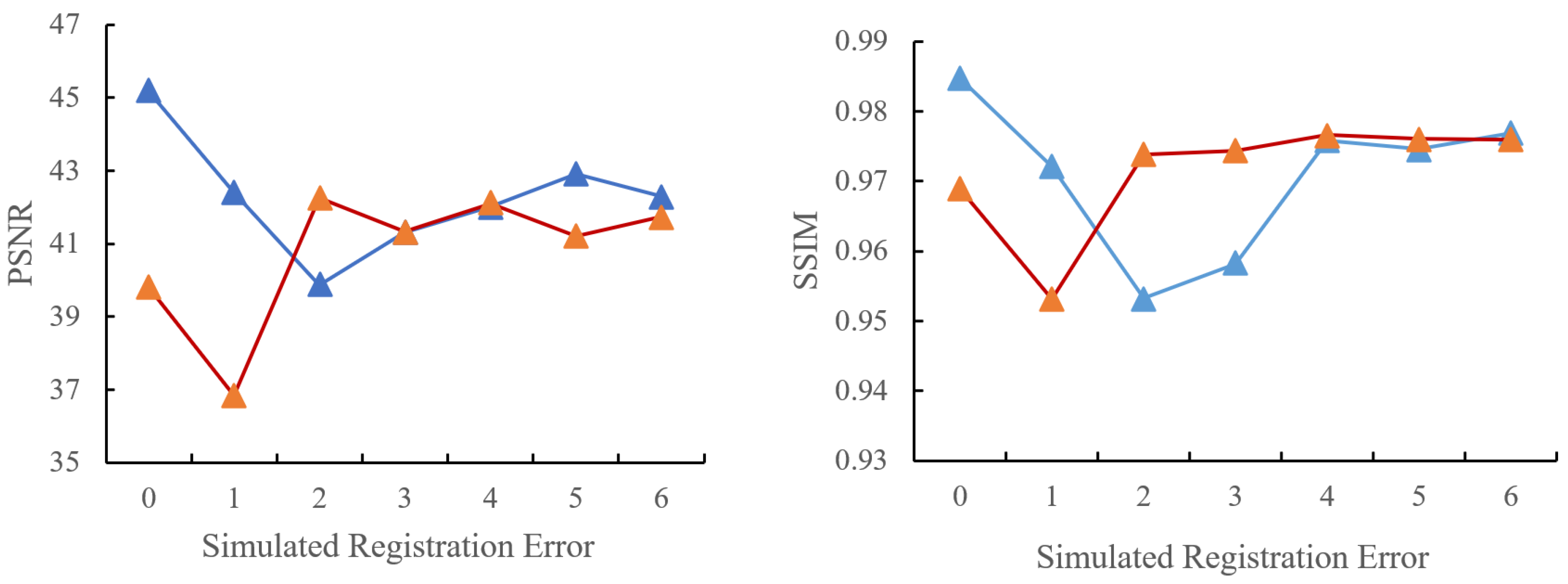
Effects of simulated registration errors on fusion

Registration errors are common in data fusion and may have great effects on fusion accuracy. Thus, resilience to registration error is important for fusion methods and spectral-super-resolution methods. In order to evaluate methods’ resistance to registration error, we set up seven experiments with simulated registration errors, ranging from 0 to 6. Simulation is conducted by moving hyperspectral data towards the x and y axes by a distance of 0 to 6. The simulation process is shown in Figure 8. The orange square represents multispectral data and these blue squares represent different groups of hyperspectral data. After simulation, seven experiment groups are established.

Seven experiments were conducted between SRE-ResNet and ResNet for the two datasets. There are 21 experiment results overall. Figure 9 and Figure 10 show the different indices results for the two datasets. They are PSNR, SSIM, RMSE and SAM. For Dataset I, SRE-ResNet and ResNet both perform well when it comes to different simulated registration errors. This proves that SRE-ResNet can restore original data without decreasing too much original spatial and spectral information. For Dataset II, SRE-ResNet outperforms ResNet in all six simulated registration errors, and still, we can come to the conclusion that SRE-ResNet can preserve information both spectrally and spatially, even when registration errors occur. We can see that ResNet results are better than SRE-ResNet in Dataset I with some registration errors. This may be due to the land cover types in the whole scene, which may affect the projection of PCA transformation. Still, however, when it comes to no registration error, SRE-ResNet performs better than ResNet overall, which makes SRE-ResNet a better choice.

(3)

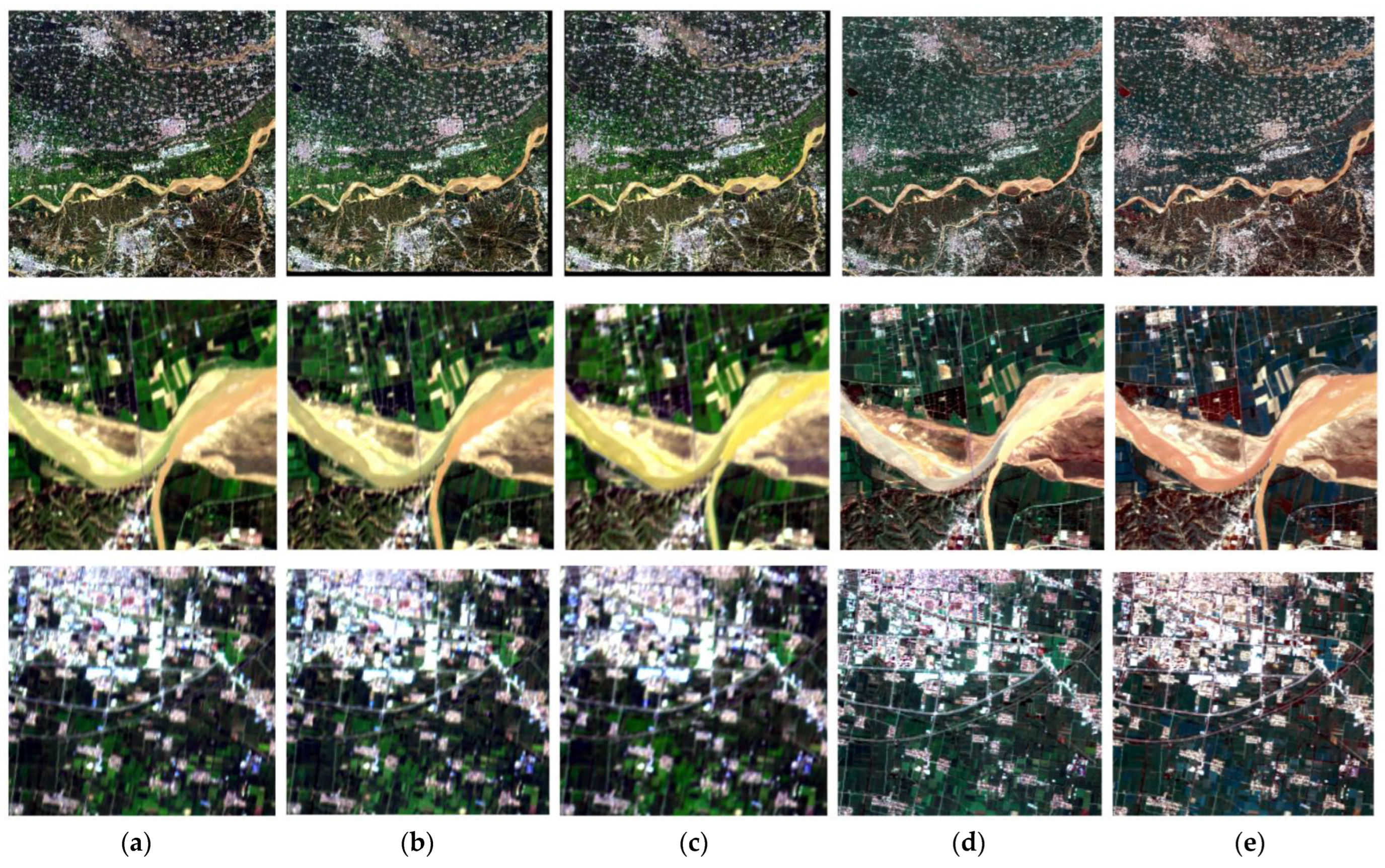
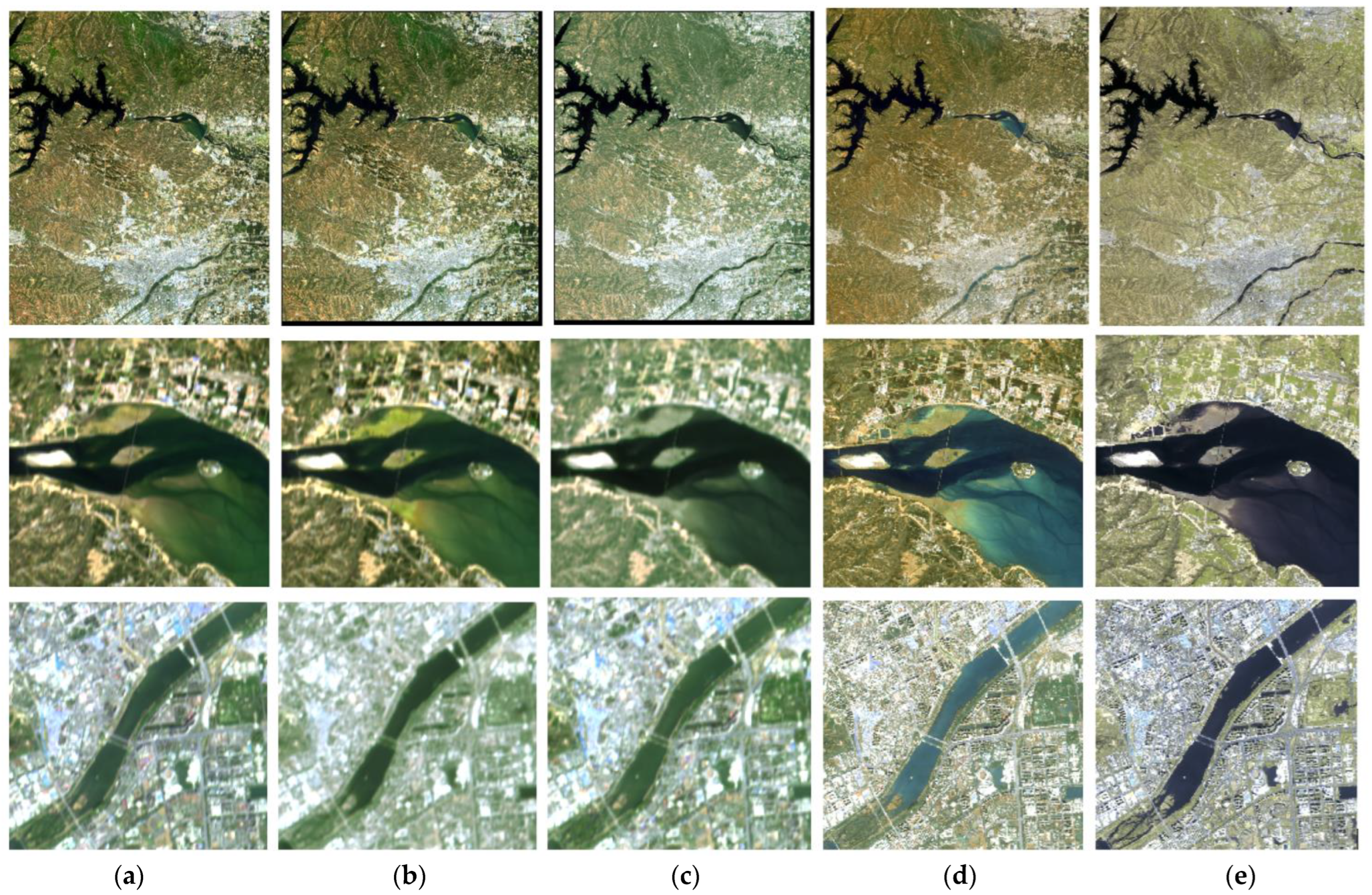
Comparison with state-of-the-art methods

In order to show the advantage of our method, we chose three spectral super-resolution methods as a comparison group. They are HSCNN, coupled nonnegative matrix factorization method (CNMF) and joint sparse and low-rank learning method (J-SLoL). HSCNN is a typical deep learning method, which first upsamples the RGB input to a hyperspectral image using a spectral interpolation algorithm. This spectrally upsampled image has the same number of bands as the expected hyperspectral output. Then, the network takes the spectrally upsampled image as input and predicts the missing details (residuals) by learning a stack of convolutional layers [28]. CNMF and J-SLoL are the traditional machine learning method. CNMF built a sensor observation model using a combination of spectral response and point spread function (PSF) and used paired non-negative matrix iterative decomposition to obtain reconstructed hyperspectral data [10]. J-SLoL spectrally enhances multispectral images by jointly learning low-rank hyperspectral–multispectral dictionary pairs from overlapped regions [26]. As J-SLoL was written in MATLAB and due to the inherent processing attributes of MATLAB, J-SLoL is not able to process large datasets. Thus, training samples were randomly chosen to be 2/3 of the overlapping areas when the model was trained. Similar to the experiment settings in (2), 0–6 simulated registration errors were set.

We calculated the fusion index of each method with seven different simulated registration errors and the results are shown in Figure 11 and Figure 12. For Dataset I, SRE-ResNet and ResNet are the best among all methods, followed by HSCNN. Judging by the slope of each line, neural network methods appear to be a flatter curve, which are more resilient to simulated registration error compared to traditional methods. Similar conclusions can also be drawn in the results of Dataset II. The reason why deep learning methods are more resilient to spatial registration error is that multilayers of convolution bring large receptive fields, which traditional methods do not possess. This brings robustness to spatial coregistration error. SRE-ResNet performed best among all methods and was more resilient to spatial registration error than other methods.

4. Results

Here, the fusion results of different methods are shown. Figure 13 and Figure 14 show the typical band for Dataset I and Dataset II. We can see that all methods can seemingly remove stripe noise in the hyperspectral data. However, SRE-ResNet shows the most similar spatial characteristics compared to the original dataset. Figure 15 and Figure 16 show RGB composite of fusion results for Dataset I and Dataset II. SRE-ResNet shows the most similar texture and tones to the original hyperspectral data. HSCNN’s result shows similar texture yet a little diffusion in tones. CNMF and J-SLoL’s results show better details than the original hyperspectral data. This is due to the fact that both CNMF and J-SLoL use paired matrices or dictionaries to characterize common information in both hyperspectral and multispectral data, rather than learning the mappings between multispectral data and hyperspectral data. Thus, it is a common inherent feature of CNMF and J-SLoL to bring multispectral spatial information into the fusion result. This may yield better results in the spatial domain, yet the hyperspectral sensor’s characteristics are partly lost. When it comes to multi-temporal applications, this may bring errors, with some scenes’ hyperspectral data being injected with multispectral data’s texture information.

Quantitative fusion evaluation results from Dataset I and Dataset II were recorded in

Table 4. Quantitative fusion evaluation results of Dataset I.

	SRE-ResNet	HSCNN	CNMF	J-SLoL
PSNR	45.18373	38.26820	37.42987	36.28148
SAM	0.03000	0.06527	0.10819	0.12937
SSIM	0.98466	0.94734	0.94292	0.90949
RMSE	34.91505	65.09146	110.92780	169.33570
Time(s)	242	415	8628	7291

and

Table 5. Quantitative fusion evaluation of Dataset II.

	SRE-ResNet	HSCNN	CNMF	J-SLoL
PSNR	42.10580	36.14708	37.93763	35.76092
SAM	0.03656	0.07635	0.09107	0.10593
SSIM	0.96790	0.90099	0.92941	0.89520
RMSE	38.83331	90.78757	71.98587	105.00250
Time(s)	346	495	13951	8327

. We can see from the table that SRE-ResNet shows the best performance in both the spatial and spectral domain. In addition, running times, including training and predicting, were also recorded. Although SRE-ResNet uses deep learning tools, this method uses the least time, which is more suitable for real applications.

5. Conclusions

The article uses SRE-ResNet to extend the swath of ZY1-02D hyperspectral data with the help of auxiliary multispectral data. The method is based on the idea of learning the mappings between multispectral data and hyperspectral data, which uses ResNet and principal component analysis (PCA). With the help of PCA, stripe noise and collage can be removed. Experiments are designed to test the effect of PCA and the method’s resilience to registration error by simulating 0–6 pixels of registration error. The results show that adding PCA can effectively improve the accuracy of swath reconstruction and resilience to registration error. SNR comparisons also show that SRE-ResNet can improve SNR, but without PCA, the SNR may decrease in some bands. SRE-ResNet was also compared with the state-of-art methods, which are HSCNN, CNMF and J-SLoL. Experiments showed that SRE-ResNet performs the best, relatively, among all the methods. Overall, training and prediction time show that SRE-ResNet uses the least time.

Thus, we can come to the conclusion that SRE-ResNet has the following advantages: (1) removes the collage effect and stripe noise in the ZY1-02D shortwave bands; (2) ignores the effect of mis-coregistration and is more applicable to real applications; (3) extends the swath of hyperspectral data; thus, it can increase the area coverage and revisit time of ZY1-02D hyperspectral data. This method is time saving, of high accuracy and more applicable to real applications.

References

1. Camps-Valls, G.; Tuia, D.; Bruzzone, L.; Benediktsson, J.A. Advances in hyperspectral image classification. IEEE Signal Process. Mag. 2014, 31, 45–54. [Google Scholar] [CrossRef] [Green Version]
2. Eismann, M.T.; Meola, J.; Hardie, R.C. Hyperspectral Change Detection in the Presenceof Diurnal and Seasonal Variations. IEEE Trans. Geosci. Remote Sens. 2008, 46, 237–249. [Google Scholar] [CrossRef]
3. Koponen, S.; Pulliainen, J.; Kallio, K.; Hallikainen, M. Lake water quality classification with airborne hyperspectral spectrometer and simulated MERIS data. Remote Sens. Environ. 2002, 79, 51–59. [Google Scholar] [CrossRef]
4. Zarco-Tejada, P.J.; Ustin, S.L.; Whiting, M.L. Temporal and Spatial Relationships between within-field Yield variability in Cotton and High-Spatial Hyperspectral Remote Sensing Imagery. Agron. J. 2005, 97, 641–653. [Google Scholar] [CrossRef] [Green Version]
5. Sun, W.; Liu, K.; Ren, G.; Liu, W.; Yang, G.; Meng, X.; Peng, J. A simple and effective spectral-spatial method for mapping large-scale coastal wetlands using China ZY1-02D satellite hyperspectral images. Int. J. Appl. Earth Obs. Geoinf. 2021, 104, 102572. [Google Scholar] [CrossRef]
6. Chang, M.; Meng, X.; Sun, W.; Yang, G.; Peng, J. Collaborative Coupled Hyperspectral Unmixing Based Subpixel Change Detection for Analyzing Coastal Wetlands. IEEE J. Sel. Top. Appl. Earth Obs. Remote Sens. 2021, 14, 8208–8224. [Google Scholar] [CrossRef]
7. Yuan, Q.; Wei, Y.; Meng, X.; Shen, H.; Zhang, L. A Multiscale and Multidepth Convolutional Neural Network for Remote Sensing Imagery Pan-Sharpening. IEEE J. Sel. Top. Appl. Earth Obs. Remote Sens. 2018, 11, 978–989. [Google Scholar] [CrossRef] [Green Version]
8. Gross, H.N.; Schott, J.R. Application of Spectral Mixture Analysis and Image Fusion Techniques for Image Sharpening. Remote Sens. Environ. 1998, 63, 85–94. [Google Scholar] [CrossRef]
9. Huang, Z.; Yu, X.; Wang, G.; Wang, Z. Application of Several Non-negative Matrix Factorization-Based Methods in Remote Sensing Image Fusion. In Proceedings of the 5th International Conference on Fuzzy Systems & Knowledge Discovery (FSKD), Jinan, China, 18–20 October 2008. [Google Scholar]
10. Yokoya, N.; Yairi, T.; Iwasaki, A. Coupled Nonnegative Matrix Factorization Unmixing for Hyperspectral and Multispectral Data Fusion. IEEE Trans. Geosci. Remote Sens. 2012, 50, 528–537. [Google Scholar] [CrossRef]
11. Hardie, R.; Eismann, M.; Wilson, G. MAP Estimation for Hyperspectral Image Resolution Enhancement Using an Auxiliary Sensor. IEEE Trans Image Process. 2004, 13, 1174–1184. [Google Scholar] [CrossRef]
12. Eismann, M.T.; Hardie, R. Resolution enhancement of hyperspectral imagery using coincident panchromatic imagery and a stochastic mixing model. In Proceedings of the IEEE Workshop on Advances in Techniques for Analysis of Remotely Sensed Data, Greenbelt, MD, USA, 27–28 October 2003. [Google Scholar]
13. Eismann, M.T.; Hardie, R. Hyperspectral resolution enhancement using high-resolution multispectral imagery with arbitrary response functions. IEEE Trans. Geosci. Remote Sens. 2005, 43, 455–465. [Google Scholar] [CrossRef]
14. ZhiRong, G.; Bin, W.; LiMing, Z. Remote sensing image fusion based on Bayesian linear estimation. Sci. China. Ser. F Inf. Sci. 2007, 50, 227–240. [Google Scholar]
15. Wei, Q.; Dobigeon, N.; Tourneret, J.-Y. Bayesian fusion of hyperspectral and multispectral images. In Proceedings of the 2014 IEEE International Conference on Acoustics, Speech and Signal Processing (ICASSP), Florence, Italy, 4–9 May 2014; pp. 3176–3180. [Google Scholar]
16. Wei, Q.; Dobigeon, N.; Tourneret, J.-Y. Bayesian fusion of multispectral and hyperspectral images with unknown sensor spectral response. In Proceedings of the 2014 IEEE International Conference on Image Processing (ICIP), Paris, France, 27–30 October 2014; pp. 698–702. [Google Scholar]
17. Li, S.; Yang, B. A New Pan-Sharpening Method Using a Compressed Sensing Technique. IEEE Trans. Geosci. Remote Sens. 2011, 49, 738–746. [Google Scholar] [CrossRef]
18. Huang, B.; Song, H.; Cui, H.; Peng, J.; Xu, Z. Spatial and Spectral Image Fusion Using Sparse Matrix Factorization. IEEE Trans. Geosci. Remote Sens. 2014, 52, 1693–1704. [Google Scholar] [CrossRef]
19. Han, C.; Zhang, H.; Gao, C.; Jiang, C.; Sang, N.; Zhang, L. A Remote Sensing Image Fusion Method Based on the Analysis Sparse Model. IEEE J. Sel. Top. Appl. Earth Obs. Remote Sens. 2016, 9, 439–453. [Google Scholar] [CrossRef]
20. Huang, W.; Xiao, L.; Wei, Z.; Liu, H.; Tang, S. A New Pan-Sharpening Method With Deep Neural Networks. IEEE Geosci. Remote Sens. Lett. 2015, 12, 1037–1041. [Google Scholar] [CrossRef]
21. Giuseppe, M.; Davide, C.; Luisa, V.; Giuseppe, S. Pansharpening by Convolutional Neural Networks. Remote Sens. 2016, 8, 594. [Google Scholar]
22. Azarang, A.; Ghassemian, H. A new pansharpening method using multi resolution analysis framework and deep neural networks. In Proceedings of the 2017 3rd International Conference on Pattern Recognition & Image Analysis (IPRIA), Shahrekord, Iran, 19–20 April 2017. [Google Scholar]
23. Wei, Y.; Yuan, Q.; Shen, H.; Zhang, L. Boosting the Accuracy of Multispectral Image Pansharpening by Learning a Deep Residual Network. IEEE Geosci. Remote Sens. Lett. 2017, 14, 1795–1799. [Google Scholar] [CrossRef] [Green Version]
24. Palsson, F.; Sveinsson, J.R.; Ulfarsson, M.O. Multispectral and Hyperspectral Image Fusion Using a 3-D-Convolutional Neural Network. IEEE Geosci. Remote Sens. Lett. 2017, 14, 639–643. [Google Scholar] [CrossRef] [Green Version]
25. Sun, X.; Zhang, L.; Yang, H.; Wu, T.; Cen, Y.; Guo, Y. Enhancement of Spectral Resolution for Remotely Sensed Multispectral Image. IEEE J. Sel. Top. Appl. Earth Obs. Remote Sens. 2015, 8, 2198–2211. [Google Scholar] [CrossRef]
26. Gao, L.; Hong, D.; Yao, J.; Zhang, B.; Gamba, P.; Chanussot, J. Spectral Superresolution of Multispectral Imagery with Joint Sparse and Low-Rank Learning. IEEE Trans. Geosci. Remote Sens. 2020, 59, 2269–2280. [Google Scholar] [CrossRef]
27. Xiong, Z.; Shi, Z.; Li, H.; Wang, L.; Liu, D.; Wu, F. HSCNN: CNN-Based Hyperspectral Image Recovery from Spectrally Undersampled Projections. In Proceedings of the 2017 IEEE International Conference on Computer Vision Workshop (ICCVW), Venice, Italy, 22–29 October 2017. [Google Scholar]
28. Shi, Z.; Chen, C.; Xiong, Z.; Liu, D.; Wu, F. HSCNN+: Advanced CNN-Based Hyperspectral Recovery from RGB Images. In Proceedings of the 2018 IEEE/CVF Conference on Computer Vision and Pattern Recognition Workshops (CVPRW), Salt Lake City, UT, USA, 18–22 June 2018. [Google Scholar]
29. Richards, A.J. Remote Sensing Digital Image Analysis; Springer: Berlin/Heidelberg, Germany, 1993. [Google Scholar]
30. Farrell, M.D.; Mersereau, R.M., Jr. On the impact of PCA dimension reduction for hyperspectral detection of difficult targets. IEEE Geosci. Remote Sens. Lett. 2005, 2, 192–195. [Google Scholar] [CrossRef]
31. He, K.; Zhang, X.; Ren, S.; Sun, J. Deep Residual Learning for Image Recognition. In Proceedings of the IEEE Conference on Computer Vision and Pattern Recognition (CVPR), San Francisco, CA, USA, 18–20 June 1996; pp. 770–778. [Google Scholar]
32. Bishop, C.M. Neural Networks for Pattern Recognition. Adv. Comput. 1993, 37, 119–166. [Google Scholar]
33. Huynh-Thu, Q.; Ghanbari, M. Scope of validity of PSNR in image/video quality assessment. Electron. Lett. 2008, 44, 800–801. [Google Scholar] [CrossRef]
34. Zhang, Y.; De Backer, S.; Scheunders, P. Noise-Resistant Wavelet-Based Bayesian Fusion of Multispectral and Hyperspectral Images. IEEE Trans. Geosci. Remote Sens. 2009, 47, 3834–3843. [Google Scholar] [CrossRef]
35. Alparone, L.; Wald, L.; Chanussot, J.; Thomas, C.; Gamba, P.; Bruce, L.M. Comparison of Pansharpening Algorithms: Outcome of the 2006 GRS-S Data Fusion Contest. IEEE Trans. Geosci. Remote Sens. 2007, 45, 3012–3021. [Google Scholar] [CrossRef] [Green Version]
36. Wang, Z. Image Quality Assessment: From Error Visibility to Structural Similarity. IEEE Trans. Image Process. 2004, 13, 600–612. [Google Scholar] [CrossRef]
37. Fiete, R.D.; Tantalo, T. Comparison of SNR image quality metrics for remote sensing systems. Opt. Eng. 2001, 40, 574–585. [Google Scholar]
Figure 1. Examples of defects in ZY1-02D hyperspectral data. (a) Band 129 (1880.13 nm), (b) band 166 (2501.08 nm).
Remotesensing 14 05890 g001
Figure 2. Basic framework of SRE-ResNet.
Remotesensing 14 05890 g002
Figure 3. ResNet structure in SRE-ResNet framework. (a) Residual Learning, (b) SRE-ResNet.
Remotesensing 14 05890 g003
Figure 4. RGB composite of fusion result comparison between SRE-ResNet and ResNet for Dataset I. (ac) are the whole scene of ground truth, prediction of SRE-ResNet and ResNet. (df) are the detailed scene of ground truth, prediction of SRE-ResNet and ResNet.
Remotesensing 14 05890 g004
Figure 5. RGB composite of fusion result comparison between SRE-ResNet and ResNet for Dataset II. (ac) are the whole scene of ground truth, prediction of SRE-ResNet and ResNet. (df) are the detailed scene of ground truth, prediction of SRE-ResNet and ResNet.
Remotesensing 14 05890 g005
Figure 6. SNR comparison between SRE-ResNet and ResNet for Dataset I. (a) SRE-ResNet, (b) ResNet.
Remotesensing 14 05890 g006aRemotesensing 14 05890 g006b
Figure 7. Quantitative fusion result comparison between SRE-ResNet and ResNet for Dataset II. (a) SRE-ResNet, (b) SRE-ResNet.
Remotesensing 14 05890 g007
Figure 8. Simulation of registration errors between hyperspectral data and multispectral data.
Remotesensing 14 05890 g008
Figure 9. Quantitative fusion result comparison between SRE-ResNet and ResNet for Dataset I.
Remotesensing 14 05890 g009aRemotesensing 14 05890 g009b
Figure 10. Quantitative fusion result comparison between SRE-ResNet and ResNet for Dataset II.
Remotesensing 14 05890 g010
Figure 11. Quality assessment result of Dataset I with different simulated registration error.
Remotesensing 14 05890 g011
Figure 12. Quality assessment result of Dataset II with different simulated registration error.
Remotesensing 14 05890 g012
Figure 13. Image of Band 125 of dataset I. (a) Original Image, (b) SRE-ResNet, (c) HSCNN, (d) CNMF, (e) J-SLoL.
Remotesensing 14 05890 g013
Figure 14. Image of Band 125 of dataset II. (a) Original Image, (b) SRE-ResNet, (c) HSCNN, (d) CNMF, (e) J-SLoL.
Remotesensing 14 05890 g014
Figure 15. RGB Composites of fusion results comparison dataset I. (a) Original Image, (b) SRE-ResNet, (c) HSCNN, (d) CNMF, (e) J-SLoL.
Remotesensing 14 05890 g015
Figure 16. RGB Composites of fusion results comparison dataset II. (a) Original Image, (b) SRE-ResNet, (c) HSCNN, (d) CNMF, (e) J-SLoL.
Remotesensing 14 05890 g016