1. Introduction
Landslides are the widely distributed and most influential geological disasters in southern China. According to statistics, a total of 7840 geological disasters occurred in China in 2020, including 4810 landslide disasters, causing 117 deaths and direct economic losses of more than 700 million dollars [
1]. Landslide disasters can be prevented at a low cost by conducting all-weather monitoring and early warning of landslides with potential risks using the Internet of Things (IoT), sensors, Remote Sensing (RS), and other technologies [
2,
3,
4]. The development of automatic monitoring technology has led to a dramatic increase in the amount of monitoring data, which also provides data support for the prediction of the evolution process of landslide displacement. It has become a research trend in recent years to fully mine the evolution characteristics of landslides in the enormous monitoring data and predict the failure process.
Landslide deformation exhibits completely non-linear characteristics and is influenced by some internal factors, such as geological structure, physical properties of soil, and material composition, as well as by external factors, such as rainfall, vibration, temperature, vegetation cover, and water circulation [
5,
6,
7,
8]. The internal factors play a decisive role among the two factors, and the external factors play an induced role. The landslide deformation will be triggered only when the internal and external factors work together. Many scholars have also proposed some models that can predict the evolution of landslide displacements based on the characteristics of these internal and external factors. The prediction based on the mechanism of landslide internal factors is called “physics-based” prediction [
9,
10,
11]. However, it is very expensive and difficult to sample and analyze various parameters inside the landslide, which makes it difficult to achieve near-real-time prediction. The prediction based on monitoring data from external factors is called “data-based” prediction. In this way, the data collection cost is relatively low, and the types and volumes of data are very rich. Therefore, more and more significant studies have used long-term monitoring data to predict landslide deformation process, especially for landslides affected by rainfall and reservoir water, which are widely distributed in southern China [
12,
13,
14,
15,
16,
17].
Modeling research on “data-based” prediction has gone through four stages: empirical models, statistical models, nonlinear models, and artificial intelligence models [
18]. In the first three stages, the proposed models are limited by the model properties and often only use cumulative displacements for analysis and prediction. Such models have no way to consider other features in the landslide deformation process, and thus, have limited prediction effects. The development of artificial intelligence, especially deep learning technology, has also provided new ideas for landslide displacement prediction in recent years. Numerous researchers have suggested a variety of models to completely account for the multi-source monitoring data connected to the landslide deformation process, and the prediction effect has significantly improved. These models can be generally classified into three major categories: machine learning prediction models, Recurrent Neural Network (RNN) prediction models, and Graph Neural Network (GNN) prediction models.
Machine learning prediction models mainly include Extreme Learning Machines (ELM) [
19,
20,
21,
22,
23], Backpropagation (BP) neural networks [
24,
25], Support Vector Machines (SVM) [
26,
27,
28,
29], and their improved models. These models are simple to implement, fast to compute, and can use multi-source monitoring data as the input to the model, effectively improving the prediction model’s ability to integrate multi-source monitoring data. However, these machine learning prediction models are often referred to as static models because they typically only take into account the input state at the current time and ignore the impact of the past state in the future. Landslide deformation is a continuous and dynamic process. The past state plays a significant role in the future state evolution of the landslide and should be considered. The RNN and Long Short-Term Memory (LSTM) realize the prediction models to “remember” and “forget” the past states by their internal gate construction to integrate the past state information into the prediction process and enhance the continuity of the prediction process. Many scholars have already developed landslide prediction models using RNN, LSTM and their improvements, and some representative models include GRU [
30], simple LSTM [
18], EMD-LSTM [
31], LMD-BiLSTM [
32], VMD-Stacked LSTM-TAR [
33], VMD-BiLSTM [
34], CEEMDAN-AMLSTM [
35], and so on. These models realize the transformation of landslide displacement prediction from static to dynamic, but there are two problems. First, RNN and LSTM only consider the temporal correlation in landslide deformation prediction, but not the spatial correlation. Landslide failures tend to respond on a larger spatial scale, so landslide monitoring also tends to deploy sensors over a larger area to obtain monitoring data on a larger spatial scale. The monitoring data from these sensors present a correlation not only in time but also in space, which helps to improve the perceptive ability and prediction effect of the prediction model on a large-scale space in the prediction model, considering spatial correlation. Because the GNN, which has emerged in recent years, can consider the spatial correlation between multiple nodes via weighted adjacency matrices, it has been used by many scholars in the field of landslide displacement prediction, and the more representative models are primarily Attentive-GNN [
36], GC-GRU-N [
37], T-GCN [
38], and so on. However, GNN requires high data integrity resulting in high data collection cost. There is a lack of complete public datasets leading to fewer applications of GNNs. Second, there is a correlation between multi-source monitoring data from different sensors in the short term before landslides occur, which cannot be considered by traditional RNN or LSTM. Lai et al. [
39] presented the Long and Short-Term Time-Series Network (LSTNet) as a solution to this problem. In LSTNet, the RNN and the Convolutional Neural Network (CNN) are combined. The CNN extracts the correlation features of the input variables, and the extracted features are then input into the RNN for prediction. Therefore, the LSTNet has good applicability and prediction effects for multivariate time series prediction problems.
The current studies on landslide displacement prediction mainly focus on deterministic point prediction, that is, predicting the specific value of landslide displacement at a certain time in the future. Few studies have explored the uncertainty of such predictions, that is, how to construct Prediction Intervals (PIs). PIs can not only reflect the deformation trend of landslide displacement in the future but also get the upper and lower bounds of predicted displacement. It is helpful for decision-makers to evaluate the uncertainty of the prediction and make more accurate decisions. Therefore, constructing PIs is more meaningful than point prediction. Conventional methods for constructing PIs include delta, Mean-Variance Estimation (MVE), and Bayesian. These methods are ineffective because they not only require that the data satisfy the Gaussian noise distribution but also that the inverse of the Hessian matrix will be continually calculated. Additionally, the Lower Upper Bound Estimation (LUBE) and bootstrap are popular because they do not make any prior assumptions. At present, there is little research on constructing PIs of landslide displacement. Lian et al. [
40,
41,
42,
43] used bootstrap and LUBE to construct PIs of landslide displacements for various machine learning models, such as ANN, ELM, SVM, and RVFLN, which were validated in several landslides in the Three Gorges reservoir area. This is the earliest study on constructing PIs for landslide displacements that can be found. Since then, Ma et al. [
44], Wang et al. [
45,
46,
47], Ge et al. [
48], and Li et al. [
49] conducted similar studies and achieved many valuable and meaningful research results. However, these current studies are based on static models of machine learning to construct PIs and have not yet considered the dynamic characteristics of time series and the correlation between input variables. The generated PIs will perform better if the bootstrap method can be used in combination with the LSTNet model to predict landslide displacement.
This study suggested a landslide displacement prediction model that combines Variational Mode Decomposition (VMD) with LSTNet to address the aforementioned problems. It also used the bootstrap to create PIs to quantify the uncertainty of the proposed model. The proposed model first decomposes the cumulative displacement into trend displacement, periodic displacement, and random displacement using the VMD algorithm. Then, an improved polynomial fitting method is employed for trend displacement prediction. The LSTNet model is employed to predict the periodic and random displacements. By summing the prediction results from the three displacements, the point prediction results of the cumulative displacement are obtained. Finally, the bootstrap method is used to evaluate the uncertainty of point prediction results and construct PIs. In this study, the Baishuihe landslide in the Three Gorges reservoir area in southern China was selected as the study case, and the monitoring data from two monitoring stations, ZG118 and XD01, were predicted using the proposed model. To verify that the proposed model is effective and competitive, its prediction results were compared to those of three baseline models: LSSVR, BP, and LSTM.
2. Methods
2.1. Time Series Decomposition
The cumulative displacements
of landslides are the coupled responses of numerous factors both inside and outside the landslide, and these coupled responses mainly consist of three parts: trend displacement
, periodic displacement
, and random displacement
, i.e.,
Among them, the trend displacement, which plays a decisive role in the process of landslide deformation, is the surface displacement response caused by internal factors, such as rock and soil properties and geological structure inside the landslide. The main characteristics are that the displacement increases monotonically with time and the time series complexity is very low. Periodic displacement is caused by external rainfall, reservoir level, and other factors, which often have seasonal periodicity, so periodic displacement also has seasonal periodicity. Random displacement is mainly the remaining residual component, which characterizes the effect of random factors such as human activities and vibration on landslide displacement.
In this study, the cumulative displacement is decomposed by the VMD algorithm with minimum sample entropy constraint. The VMD [
50] is an adaptive and fully non-recursive signal processing method that can adaptively match the optimal center frequency and finite bandwidth of each mode to achieve the effective separation of the Intrinsic Modal Functions (IMFs) and the division of the signal frequency domain, and then obtain the effective decomposition components of the signal. The core idea of VMD is to construct and solve the variational problem. Assuming that the original signal
will be decomposed into
components, the corresponding constrained variational expressions are:
where
denotes the decomposed components,
denotes the actual center frequency of each IMF component,
denotes the Dirac function, * denotes the convolution operation,
denotes the analyzed signal of each component, and
denotes the estimated center frequency of each analyzed signal.
The Lagrangian multiplication operator
is introduced to solve Equation (2), thus, transforming the constrained variation problem into an unconstrained variation problem. We have:
where
is the penalty factor, which can effectively reduce the interference of Gaussian noise. The alternating direction multiplier iterative algorithm is used to solve it iteratively. The core equations of the algorithm are as follows:
where
is the noise tolerance, and
,
,
, and
correspond to the Fourier transforms of
,
,
, and
, respectively. The final
and
are output when the convergence criterion of the following equation is satisfied by iterating
,
, and
through Equations (3)–(6) continuously.
where
is the accuracy convergence criterion. For the decomposition of the landslide cumulative displacement using VMD, three IMFs can be obtained by setting
= 3, which just corresponds to trend displacement, periodic displacement, and random displacement [
51,
52].
2.2. LSTNet
For the prediction problem of multivariate time series, Lai et al. [
39] proposed the LSTNet deep learning model, and the structure of this network is shown in
Figure 1. For a multivariate time series, the LSTNet network first uses a sliding window approach to create the dataset. Then, a CNN layer is used to extract short-term dependence patterns and local characteristics among the variables, and a recurrent and recurrent-skip layer is used to capture the long-term dependence patterns. The final prediction results are obtained by summing the output of the fully connected layer with the output of the traditional autoregressive model, which can be used to solve the problem of scale insensitivity of traditional models.
2.2.1. Sliding Window and Dataset Processing
Original time series must be organized according to the study purpose because they cannot be utilized directly as inputs and outputs for deep learning models. At present, the sliding window approach is the most popular technique. For a time series, the data are captured at a fixed time interval from the beginning of the time series, and this interval is called the “window”. This window continuously moves towards the end at a specific time step and continuously captures the data in the window. This process is called “sliding”. Compared with the processing method that only relies on the current moment’s monitoring data as the input, the sliding window approach fully takes into account the dynamic process of the previous period and has more sufficient information. After processing by the sliding window approach, the original time series can be transformed into a dataset for LSTNet model training and prediction.
For the created deep learning dataset, the training dataset and the test dataset should be divided according to a certain ratio. Additionally, due to the inconsistency in magnitude between the input features, the training dataset should be normalized with the following equation:
where
denotes the normalized data,
denotes the unnormalized data,
denotes the maximum value, and
denotes the minimum value.
All training data are scaled between 0 and 1 after normalization. It should be emphasized that data normalization can only be performed on the training dataset after the dataset has been divided. If normalization is performed on the unsegmented dataset, the information from the training dataset will leak into the test dataset, and such results are unreliable.
2.2.2. Convolution Layer
For each sample in the created dataset, LSTNet first uses a convolutional neural network without pooling to obtain short-term patterns and local dependencies between variables. The convolution kernel used in the convolution layer is calculated with the input multidimensional time series according to the following equation:
where ∗ represents the convolution operation,
denotes the convolution kernel weight matrix,
denotes the input multidimensional time series feature matrix,
denotes the bias weight,
denotes the output vector, and
is the activation function.
2.2.3. Recurrent and Recurrent-Skip Layer
The recurrent and recurrent-skip layers instantly take the output of the convolutional component as their input. To better capture the long-term dependence patterns of the time series, LSTM units are used in the recurrent layer in this study instead of the GRU units used by Lai et al. [
39] In comparison to traditional RNN, the LSTM designs the forget gate, input gate, output gate, and memory unit to achieve the removal and addition of past information, thus, resolving the long-term dependency problem of conventional RNN. The input gate can control which information will be input into the memory cell. The forget gate can control which information in the memory cell will be deleted for “forget”, and the output gate can control which information will be passed to the hidden state of the next LSTM cell. The forward calculation process of the LSTM is as follows:
where
,
,
denote the values of input gate, forget gate and output gate, respectively;
denotes the value of memory cell;
,
,
, and
denote their corresponding biases, respectively.
denotes the weight between input node and hidden node,
denotes the weight between hidden layer and memory cell,
denotes the weight between memory cell to output node.
LSTM can capture the dependency patterns of long-term sequences by “memory” and “forget”. However, as the length of time series increases, the gradient gradually decreases or even disappears, and the ability of LSTM to capture ultra-long-term dependency patterns decreases sharply or even disappears. Therefore, Lai et al. [
39] proposed increasing the network’s ability to capture ultra-long-term dependency patterns by adding a recurrent-skip layer. The update process for the recurrent-skip layer can be expressed as:
where the parameter
is generally equal to the average period length of the time series,
denotes the value of the memory cell before
time steps, and
denotes the state of the hidden layer before
time steps. The prediction problems of time series with a steady period are better suited for this recurrent skip layer. Since most landslides in south China are influenced by seasonal rainfall and the deformation velocity characteristics are periodic, LSTNet has strong application.
A fully connected layer is required at the end of LSTNet to integrate the output of the hidden states of the recurrent and recurrent-skip layers. The calculation formula is as follows:
where
denotes the hidden state of the recurrent component.
denotes the hidden state of the recurrent skip component.
denotes the output.
and
are the weights to be learned, and
denotes the bias to be learned.
2.2.4. Autoregressive Component
Both CNN and RNN are fully nonlinear deep learning networks with poor scale sensitivity to the input features. To alleviate the scale insensitivity problem, an autoregressive (
AR) path is added to LSTNet.
AR can be viewed as a multiple linear regression model. The forward calculation formula is as follows:
where
denotes the output of the
AR component,
denotes the input of the
AR component,
and
denote the autoregressive coefficients and bias of the
AR component.
The final output of LSTNet is the sum of the outputs of the
AR component, and the recurrent and recurrent-skip component, which is:
2.3. Bootstrap and PI
According to Equation (1), the cumulative displacement can be expressed as the sum of trend, periodic, and random displacements. When the proposed model is used for landslide displacement prediction, each displacement component is used with different characteristics, so Equation (1) can be rewritten as:
where
is the output at the
moment.
and
are the predictions of the trend displacement and the periodic displacement at the
moment.
denotes the prediction of the random displacement, which can generally be assumed to obey a standard normal distribution.
,
and
are the input feature matrixes used to predict the trend displacement, the periodic displacement, and the random displacement, respectively. Assuming that the estimated outputs of the prediction models for trend displacement and periodic displacement are
and
, respectively, the overall prediction error can be expressed as:
According to Ma et al. [
44] and Jiang et al. [
53], the errors of the prediction model are statistically independent; then, the variance
of the total error of the prediction model can be expressed as:
where
,
and
denote the variance of the errors in the predicted trend displacement, periodic displacement, and random displacement, respectively. Since the improved polynomial regression prediction model used for the prediction of trend displacement is a deterministic prediction model, and the
input for each prediction is also fixed, the
is 0. For a specific significance level
, the prediction interval
with a confidence level of
can be expressed as:
where
and
are the lower and upper bounds of PI, respectively, and the calculation formula is as follows:
where
is the critical value of the standard normal distribution.
In this research, the bootstrap method is used to create and evaluate PI, which mainly includes three parts: pseudo-dataset generation, model training, and PIs construction (
Figure 2). Taking periodic displacement prediction as an example, in the pseudo-dataset generation part, the original dataset
is first normalized and divided into the training dataset and test dataset. Then, the bootstrap method is used for repeated sampling of the training dataset, and B pseudo-datasets are generated. In the model training part, B LSTNet models are first trained separately using B pseudo-datasets. After that, the test dataset of the original dataset
is predicted, and the output of the
model is
. The same method is used for the random displacement data dataset
and the model output is denoted as
. The final mean and variance of the cumulative displacement predictions for each of the B models can be obtained, respectively, as follows:
By combining Equations (29) and (30) with Equations (27) and (28), the PI under a specific confidence level can be obtained, where can be used as the result of point prediction.
2.4. Sample Entropy
Sample entropy is an evaluation index to measure the complexity of time series. For a time series , the sample entropy can be calculated as follows:
Step 1: Select a window of length and use the sliding window approach to generate a set of vector sequences with dimension , where .
Step 2: Define as the value with the largest absolute value of the difference between the corresponding elements of and .
Step 3: Given a minimum distance threshold
, define
as the number of elements satisfying
, then, we have:
Step 4: Make
, repeat Step 1 to Step 3; then, we can get:
Step 5: Calculate the sample entropy using the following equation:
When N is a finite and deterministic value, it can be estimated by the following equation:
2.5. The Proposed PI Construction Algorithm for Landslide Displacement
Figure 3 shows the specific flow diagram of bootstrap–VMD–LSTNet proposed in this paper, which mainly includes three parts: data preprocessing, feature engineering, and training and prediction.
In the data preprocessing part, the original monitoring data, such as cumulative displacement, rainfall, and reservoir level, need to be preprocessed first, mainly including anomaly detection and rejection, missing data interpolation, and equal time interval processing. Then, the processed data are used to construct the feature factor’s database and displacement target’s database for the subsequent steps.
In the feature engineering part, the cumulative displacement after data preprocessing is decomposed by the VMD algorithm to obtain trend displacement, periodic displacement, and random displacement. The feature factors are decomposed into low-frequency components and high-frequency components. Then, the grey relational analysis algorithm is used to calculate the grey relational degree between the low-frequency component and the periodic displacement and the grey relational degree between the high-frequency component and the random displacement, respectively, so as to select the factors with the higher correlation as the input feature of the LSTNet model.
In the training and prediction part, an improved polynomial function fitting algorithm is used to predict the trend displacement, and the improved measure is to determine the best power by combining the sample entropy and threshold. The low-frequency components of the selected feature factors are employed as input features for the prediction of periodic displacement. The high-frequency components of the feature factors are employed as the model’s input features for the prediction of the random displacement. Finally, the predicted trend displacement, periodic displacement, and random displacement are summed to the final point prediction result. To assess the uncertainty of such point predictions, the bootstrap method was used to analyze the mean and variance of the predicted periodic displacement and random displacement, and then to construct the PIs.
The monitoring data from the Baishuihe landslide in the Three Gorges reservoir area are used for predictions in this paper, and the proposed bootstrap–VMD–LSTNet model is compared with three baseline models, LSSVR, BP, and LSTM, to validate model performance.
2.6. Model Performance Evaluation
This study mainly consists of two parts: point prediction and interval prediction. Different evaluation indexes should be used to evaluate the prediction effect. For point prediction, the three main indexes, RSME, MAE, and R
2, are used and calculated as follows:
where
denotes the measured value,
denotes the predicted value, and
denotes the average value.
For interval prediction, Prediction Interval Coverage Probability (PICP) and Mean Prediction Interval Width (MPIW) are mainly used as evaluation indexes. The calculation formula is as follows:
where
is the number of samples in the test dataset, and
is a Boolean-type variable. The PICP describes the reliability of PI. A higher PICP means a higher reliability of PI. A lower MPIW value indicates a narrower PI and higher quality. However, when it comes to the actual application, PICP and MPIW frequently appear to be in conflict, meaning that increasing one index must occur at the expense of raising the other. The Coverage Width-Based Criterion (CWC), which was developed to address this issue, is defined as follows:
where
are generally consistent with the confidence level. When
is taken as 0, the exponential term in CWC is eliminated, and CWC is exactly equal to MPIW. Conversely, the exponential term is retained, where the penalty parameter is, to sharply amplify the difference between PICP and CWC, which leads to the rapid amplification of CWC.
3. Study Area: Baishuihe Landslide
3.1. Geological Conditions
The Baishuihe landslide is located in Shazhenxi Town, Zigui County, Yichang City, Hubei Province, China (longitude: 110°32′09″, latitude: 31°01′34″), in a wide river valley on the south bank of the Yangtze River, 56 km upstream of the Three Gorges Dam (
Figure 4). The landslide has a north–south length of 600 m, an east–west width of 700 m, an average thickness of 30 m, and a volume of 1.26 × 10
7 m
3. The terrain of the landslide is shown in
Figure 5, which generally presents a ladder shape of “high in the south and low in the north”. The trailing edge of the landslide is about 410 m, the leading edge is adjacent to the Yangtze River, and the slope is about 30°. The geological profile of the 2-2’ survey line in
Figure 5 is shown in
Figure 6, and the landslide belongs to an accumulation landslide and bedding slope. The upper part of the Baishuihe landslide is mainly Quaternary sediments, including gravelly soil and silty clay; the lower part is bedrock composed of Jurassic silty mudstone, silty siltstone, and siltstone, with a bedrock dip of 36° and a direction of 15°; the interface between the bedrock and the overburden is the sliding surface.
The Baishuihe landslide is an ancient landslide which is frequently revived. The Global Positioning System (GPS) was used to track the surface displacement of the landslide since the landslide deformation became obvious following the first impoundment of the Three Gorges Dam in June 2003.
Figure 5 shows the location of the monitoring stations, where eleven GPS surface displacement monitoring stations are placed on the landslide’s four monitoring profiles. The GPS monitoring station mainly includes a Tianbao GPS receiver, a DTU communication module, a battery, and so on. The plane accuracy of displacement measurement is 5 mm ± 1 ppm. The data collection frequency is once a month. If abnormal acceleration occurs, the collection frequency will be accelerated. Rainfall monitoring data for the Baishuihe landslide were obtained from the Zigui County Meteorological Bureau’s Shazhenxi Station, and the specific location is shown in
Figure 4a.
3.2. Deformation Characteristics
According to the crack distribution and monitoring data, the warning area of the Baishuihe landslide can be delineated as shown in
Figure 5 and
Figure 6. The deformation of two monitoring stations, ZG118 and XD01, in the warning area is very representative, and the data from these two stations are more complete than other monitoring stations during the monitoring period from January 2007 to December 2012, so the monitoring data from these two stations are selected for subsequent analysis and prediction studies (
Figure 7). The data were provided by the National Cryosphere Desert Data Center of China. From
Figure 7, it can be found that the deformation process of the Baishuihe landslide has several distinctive features, as follows:
The data curves of displacement, rainfall, and reservoir level of the Baishuihe landslide show strong temporal correlation with each other. The displacement curves of the two monitoring stations are relatively similar in shape; not only do they show a step-like characteristic, but also the change in deformation rate shows synchronization. Each of the accelerated deformation processes at both monitoring stations occurred during the rainy season from May to September each year, while the landslide deformation was slow or even non-deformed during the dry season from October to April of the next year. This indicates that the stability of the landslide is closely related to rainfall infiltration. Spatially, the displacement of monitoring station ZD01 is significantly larger than that of monitoring station ZG118, indicating that the deformation of the landslide is spatially heterogeneous, and the degree of deformation on the east side is larger than that on the west side.
The reservoir level fluctuated between 145 m and 155 m until August 2008, during which the cumulative displacement of the landslide was nearly 1 m. After August 2008, the reservoir level increased sharply and remained between 145 m and 175 m. The landslide also underwent a series of accelerated displacement processes. In terms of time, each accelerated deformation occurred after the reservoir water level dropped, presumably because the rise and fall of the water table inside the landslide lagged behind the reservoir water level change, and an outward hydrodynamic pressure was formed inside the landslide after each reservoir water level drop, resulting in a decrease in landslide stability.
Based on the comprehensive analysis of the above two characteristics, it can be considered that the external inducing factors of the Baishuihe landslide deformation are mainly rainfall infiltration and the change in reservoir water level.
4. Results
4.1. Feature Engineering
4.1.1. Constructing Feature Factors Database
In order to get better prediction results, it is necessary to select features with more significant relevance to the prediction targets to build the feature factor database, i.e., feature engineering. The purpose of this study is to predict the cumulative displacement of a landslide using multi-source monitoring data. The cumulative displacement of landslides is the coupled response of trend displacement caused by internal factors, periodic displacement caused by external factors, and random displacement caused by random factors. The targeted enhancement of each displacement prediction can improve the overall cumulative displacement prediction.
By analyzing the deformation characteristics of the Baishuihe landslide, the external factors inducing the deformation of the Baishuihe landslide are rainfall infiltration and the change in reservoir water level. Rainfall infiltration is a continuous and slow process. The intensity and duration of rainfall and even historical rainfall events will affect the deformation of landslides. In this study, the four characteristics of cumulative rainfall for the current month (), maximum daily rainfall for the current month (), maximum continuous effective rainfall for the month (), and cumulative rainfall for two months () were selected as the characteristic factors representing rainfall. For the reservoir water level factors, the change in water level has a more significant impact on landslide deformation than the water level itself. Therefore, the change in water level in the current month (), the change in maximum daily water level in the current month (), and the change in average water level in the current month compared with the previous month () were selected to represent the feature factors of reservoir water level in this study.
The internal state of a landslide is the determining factor for landslide deformation. However, it is very difficult to collect monitoring data for various parameters inside the landslide. The multi-physics field theory of landslides suggests that the deformation field of a landslide is the external expression of the coupling action of multiple physical fields in the structural field of the geological body [
54]. The size and distribution of the deformation field and its changes reflect the degree and effects of the coupling action between the structural field of the geological body and various physical fields, so the deformation field already contains the internal state information of the landslide. It has also been shown that when a landslide is in a stable state, extremely large external excitation may not have any effect [
51,
52]. However, when the landslide is in an unstable state, a very small external excitation may initiate the deformation process of the landslide. Therefore, the deformation field data of the landslide in the past period can be used as the feature factors of the internal state. In this study, three deformation field features of the current month’s displacement increment (
), two-month displacement increment (
), and three-month displacement increment (
) are selected to represent the internal state of the landslide.
4.1.2. Decomposition of Cumulative Displacement
The landslide cumulative displacement is the comprehensive response of the coupling effect of internal and external factors, and better prediction results can be obtained by predicting the response generated by both separately. According to Liu et al. [
51], Guo et al. [
52], it is necessary to decompose the monitoring data before splitting the dataset to prevent information from the training dataset leaking into the test dataset. For the cumulative displacements of ZG118 and XD01, the monitoring data of the first 60 months (January 2007–December 2011) were used as training samples, and the monitoring data of the last 12 months (January 2012–December 2012) were used as test samples. In this study, VMD is used to decompose the cumulative displacement into three components: trend displacement, periodic displacement, and random displacement. The trend displacement reflects the internal state of the landslide, the periodic displacement reflects the action of external factors, and the random displacement is the remaining decomposition component. In order to accurately obtain the three IMFs to match the three displacement components obtained from the decomposition, the parameter
in the VMD algorithm is set as 3. The trend displacement represents the long-term evolutionary trend of the landslide, and the complexity of its time series should be the lowest, that is, its sample entropy should be the smallest. Therefore, the best penalty parameter α can be determined by the optimization algorithm. In this study, α was determined to be 1.20 for ZG118 and 1.25 for XD01 by the violent trial calculation. Other parameters refer to the study by Liu et al. [
51] and Guo et al. [
52]. The time step is set as 0.1, the central frequency is initially set as 0, the termination condition is set as 10
−6, and all the omegas are started in a uniformly distributed manner.
The decomposition results of the cumulative displacements of ZG118 and XD01 are shown in
Figure 8. It can be found that the trend displacement characterized by the overall deformation trend of the landslide shows obvious monotonicity and low complexity of the time series. The periodic displacement shows an obvious and stable fluctuation period, with the peak in the rainy season and the trough in the dry season, indicating the contribution of external hydrological factors to the landslide displacement. The random displacement has no stable period and shows an obvious randomness.
4.1.3. Decomposition of the Triggering Factors
According to Liu et al. [
51] and Guo et al. [
52], the proposed model’s prediction can be improved by using the high-frequency component and low-frequency component obtained from the decomposition of the feature factors in place of the total value of the feature factors as the input features. In this study, the VMD algorithm is still used to decompose the feature factors, and the number of IMFs is set as two. The penalty factor α is determined optimally using a violent trial calculation, and the objective function of the trial calculation is to minimize the sample entropy of the low-frequency components obtained by the decomposition. Other parameters are the same as in the previous section. The decomposition results of the rainfall factors and reservoir factors are shown in
Figure 9. It can be found that the period and amplitude of the low-frequency component curves obtained from the decomposition of the feature factors are more stable and have some similarity with the curves of the periodic displacements, so the low-frequency components of the feature factors can be used as the input features of the periodic displacements. The curves of the high-frequency components fluctuate drastically without obvious periods and have some similarity with the curves of the random displacements, so the high-frequency components of the feature factors can be used as the input features of the random displacements.
4.1.4. Grey Relational Analysis
In deep learning, different features of the same dataset have different effects on the model. Before making deep learning predictions, it is necessary to select the features that are very important for the prediction results, and this process is called feature selection. Feature selection is an important part of feature engineering, which directly determines the prediction results. For each feature in the feature factors database, grey relational analysis was used to calculate the GRDs between the decomposition components of the feature factors and the displacement components, respectively, and the calculation results are shown in
Table 1. Factors with GRD greater than 0.6 are usually considered as input features for deep learning models. From
Table 1, it can be found that all factors have GRD greater than 0.6, so all these factors can be used as input features for the proposed model.
4.2. Predicted Prediction Results
4.2.1. Prediction of Trend Displacement
A landslide’s internal geological condition mostly determines its trend displacement, which has a smooth curve, low time series complexity, and small sample entropy. As a result, the least squares fitting polynomials have been used for prediction in a variety of studies [
18,
51,
52,
53]. However, the Runge phenomenon often occurs in polynomial function fitting, that is, as the power of the interpolation polynomial increases, the fitting error at the edge of the interpolation interval will become larger and larger. An improved algorithm combining time window and threshold is proposed in this study to solve this problem. The main goal of the algorithm is to make the difference between the coefficients of the highest power term of the polynomial to be solved and the coefficients of the next highest power term less than a certain threshold to avoid the presence of high-power terms, thus, avoiding the Runge phenomenon as much as possible. The algorithm’s specific flow is as follows:
Step 1: Given a time window , the last time steps of the training dataset are used as the training data to make the prediction more focused on the recent landslide deformation state. The initial highest power is set as 1, and the threshold is set as 0.1.
Step 2: Construct a polynomial function with the highest power , fit the training data by the least squares method, and calculate the coefficients of each item in the polynomial.
Step 3: Calculate the absolute value of the difference between the coefficient of the highest power term and the coefficient of the second-highest power term. If is less than the set threshold , the calculation is stopped; otherwise, the highest power is increased by 1, and Step 2 and Step 3 are repeated.
Step 4: Using the polynomial obtained in Step 3 to predict the test dataset, we can obtain the prediction results of trend displacement.
The polynomial functions fitted to the trend displacements of ZG118 and XD01 by the improved algorithm are Equations (42) and (43), respectively, and the prediction results for the test dataset are shown in
Figure 10. Although we cannot quantitatively evaluate the prediction results because we cannot get the test data of the decomposition component in the strict mode, it can be found from
Figure 10 that the prediction results of the two monitoring stations have well continued the monotonically increasing characteristics of trend displacement, which is in line with reality.
4.2.2. Prediction of Periodic Displacement
The low-frequency components of the feature factor decomposition can be used as the input features of the periodic displacement prediction model. In this section, we construct the LSTNet prediction model based on
Section 2.3, and then use a random search algorithm to determine the best hyperparameters for the model:
ZG118: The time step is set as 35, the number of the recurrent layers is set as 190, the parameter of the recurrent-skip layers is set as 11, the number of recurrent-skip layers is set as 142, the number of convolutional layers is set as 119, and the convolutional kernel is set as 5.
XD01: The time step is set as 35, the number of the recurrent layers is set as 69, the parameter of recurrent-skip layers is set as 13, the number of recurrent-skip layers is set as 65, the number of convolutional layers is set as 147, and the convolutional kernel is set as 9.
The loss function is set as MSELoss. The epochs are set as 5000, the learning rate is dynamically adjusted during the training process, the initial learning rate is 0.001, and the learning rate is changed to half of the original rate every 1000 epochs.
To evaluate the uncertainty of the trained prediction models, 200 pseudo-training sets were first generated using the bootstrap method with put-back sampling of the training set. These 200 pseudo-training sets were then used to train 200 models, each of which made predictions on the test set. Finally, the prediction results at each time step are analyzed and PIs are calculated (
Figure 11).
According to
Figure 11, the predicted values for ZG118 and XD01 are clustered close to the mean at each time step, and the predicted results furthest from the mean have a smaller probability of occurring, showing a better normal distribution. Taking the mean value as the point prediction result, it can be found that the predicted periodic displacement shows a good periodic characteristic. The peaks of the predicted periodic displacement curves are mainly distributed in the rainy season and the troughs are mainly distributed in the dry season, which is also consistent with the actual situation. Compared with the traditional point prediction, the interval prediction provides an uncertainty description of the point prediction results, which enhances the reliability of the prediction results.
4.2.3. Prediction of Random Displacement
The high-frequency components obtained from the feature factors can be used as input features for the random displacement prediction model. In this section, the random search algorithm is also used to determine the best hyperparameters of the prediction model:
ZG118: The time step is set as 35, the number of the recurrent layers is set as 88, the parameter of recurrent-skip layers is set as 14, the number of recurrent-skip layers is set as 137, the number of convolutional layers is set as 73, and the convolutional kernel is set as 3.
XD01: The time step is set as 35, the number of the recurrent layers is set as 58, the parameter of recurrent-skip layers is set as 17, the number of recurrent-skip layers is set as 130, the number of convolutional layers is set as 62, and the convolutional kernel is set as 10.
The loss function is set as MSELoss. The epochs are set as 5000. The learning rate is dynamically adjusted during the training process. The initial learning rate is 0.001, and the learning rate is changed to half of the original rate every 1000 epochs.
The bootstrap was also used for point prediction and uncertainty analysis of random displacements, and the results are shown in
Figure 12. It can be found from
Figure 12 that the prediction results of random displacements of ZG118 and XD01 at different time steps also show normal distribution characteristics. From the upper and lower bounds of the box plots, the distribution range of ZG118 is mainly ±10, and that of XD01 is mainly ±15. On the whole, it presents the random feature with 0 as the mean, which represents the error distribution of the decomposition residual components.
4.2.4. Prediction of Cumulative Displacement
The point prediction and interval prediction results of ZG118 and XD01 can be obtained according to
Section 2.5. The statistical results of the predicted cumulative displacements on the test dataset are shown in
Figure 13, and the calculated evaluation indexes of the point prediction and interval prediction for the two monitoring stations are shown in
Table 2. According to
Figure 13 and
Table 2, in terms of point prediction, the RMSE, MAE, and R
2 of the prediction model proposed in this study on ZG118 are 12.90, 11.03, and 0.95, respectively, and those on XD01 are 23.09, 17.76, and 0.96, respectively. It shows that the model proposed in this paper can well predict the specific value of cumulative displacement. In addition, the point prediction results can well reflect the accelerated deformation process of the landslide in the rainy season from May to September, and the prediction results are consistent with the actual situation.
In terms of interval prediction, the PICP of PIs of the two monitoring stations is 100% at 95% and 99% confidence levels. At a 90% confidence level, the PICP of ZG118 is also 100%, while XD01 also reaches 91.7%.
Figure 13b shows that the predicted value not included in the PI is the predicted displacement value of July 2012, but it does not exceed the PI too much. These indicate that the PIs obtained by the model proposed in this study are very reliable. The MPIW of both monitoring stations showed a certain degree of increase with the increase in the confidence level. However, even at the 99% confidence level, the MPIW of ZG118 did not exceed 100 mm, and that of XD01 was only about 150 mm, indicating that the quality of PIs was also very good.
4.3. Comparison with the Other Prediction Models
To further validate the performance of the proposed models, the three baseline models of LSSVR, BP, and LSTM were trained and predicted using the same method for the same dataset. The hyperparameters of the three baseline models were still determined using the random search method, and the prediction results are shown in
Figure 14, and the evaluation indexes are shown in
Table 2. From
Figure 14, it can be found that although the three baseline models can also basically realize the point prediction and interval prediction of landslide displacements, they have advantages and disadvantages in different evaluation indexes.
In terms of point prediction, although LSTNet, LSTM, BP, and LSSVR can all predict the cumulative displacement of ZG118 and XD01 with good intuitive effect, the prediction effect of LSTNet is significantly better than the other three baseline models from the perspective of objective evaluation indicators such as RMSE, MAE, and R2. The prediction effect of LSTM is slightly better than BP, and the prediction effect of LSSVR is the worst.
In terms of interval prediction, when the confidence level is 90%, 95%, and 99%, the PICP of LSTNet outperforms the other three baseline models. The PICP of LSTM is the same as that of LSSVR, while the PICP of BP is the worst, indicating that the PI’s reliability obtained by LSTNet is the highest, followed by LSTM and LSSVR. BP has the worst reliability. In terms of MPIW and CWC indicators, although the MPIW of BP is the smallest at 90%, 95%, and 99% confidence levels, the lower PICP leads to a sharp increase in CWC, and the comprehensive performance is not as good as other models. The MPIW of LSTNet is smaller than that of LSTM and LSSVR, and the comprehensive performance of CWC is the best because of the higher PICP, indicating that the PIs obtained by LSTNet have not only a higher reliability but also a higher quality. In addition, the MPIW of LSTM is smaller than that of LSSVR, indicating that it is necessary for the prediction process to consider the continuity of time steps. In summary, LSTNet performs better than the baseline model in both point prediction and interval prediction.
5. Discussion
With the continuous development of landslide monitoring technology in the direction of automation, low-cost, and innovation, landslide monitoring data in the future will certainly become more multi-source, massive, and complex. It is an inevitable development direction in the future to use deep learning technology to fully mine massive and multi-source monitoring data and realize the future evolution prediction of landslides. Current research mainly focuses on the point prediction of landslide displacement, that is, predicting the specific value of cumulative displacements in the future period, but the point prediction does not consider the uncertainty of the prediction process. Compared with point prediction, interval prediction can provide richer and more reliable information to decision-makers. However, the current research on interval prediction mainly focuses on static models based on machine learning, which do not consider the dynamic characteristics of time series and the correlation between multivariate variables.
In this study, a landslide displacement prediction model based on VMD and LSTNet was proposed, and the PIs of cumulative landslide displacement were constructed by the bootstrap method. The cumulative displacement prediction results of ZG118 and XD01 of the Baishuihe landslide in the Three Gorges reservoir area show that the proposed model is not only better than the LSSVR, BP, and LSTM baseline models in point prediction, but also better than other baseline models in the reliability and quality of PIs constructed.
The core of the model proposed in this study is LSTNet. Compared with LSSVR, BP, and LSTM, the advantages of LSTNet are mainly reflected in four aspects: First, compared with LSSVR and BP, LSTNet improves its learning ability for time series continuity features through the internal recurrent and recurrent-skip layers. Second, compared with LSTM, LSTNet adds a recurrent-skip component to improve its ability to capture the long-term dependence of time series. Third, LSTNet extracts the short-term, local dependencies between the input variables through the convolutional layer, which enhances its learning ability for the short-term, local features of the time series. Fourth, the presence of the autoregressive layer makes LSTNet sensitive to the input feature scales.
In addition to the use of LSTNet, the proposed model has been optimized in several aspects in order to obtain higher accuracy and more reliable predictions. First, the VMD algorithm is used to decompose the cumulative displacement into trend displacement, periodic displacement, and random displacement. This processing method decomposes the coupled, complex prediction targets into multiple prediction targets with different physical meanings, thus, improving the cumulative displacement prediction effect by enhancing the prediction effect of each target. Second, the VMD algorithm using the minimum sample entropy constraint also decomposes the feature factors into low-frequency and high-frequency components as well, while using grey relational analysis to filter out features that are more relevant to the prediction targets, which has a positive effect on improving the prediction ability of the model. Finally, for the prediction of trend displacement, an improved algorithm combining time window and threshold is used to determine the best power to avoid the Runge phenomenon in polynomial fitting prediction.
Although the point prediction and interval prediction abilities and effectiveness are enhanced by the proposed model for landslide cumulative displacement prediction in this study using a variety of optimization techniques, further research is still required in three areas. First, the recurrent-skip layer requires a good periodicity for prediction targets, and the determination of the period has a significant impact on the prediction results. Relying on subjective experience to determine is not universal, and the introduction of the attention mechanism in this part can be considered in the future to determine the period adaptively by learning. Second, the proposed model is suitable for the medium- and long-term displacement prediction of landslides affected by rainfall and reservoir levels, and the short-term prediction effect of daily-scale or hourly scale monitoring data lacks verification because of the lack of actual measurement data. In the future, sufficient time is needed to collect data to carry out validation work on prediction effects and to optimize for sample imbalance in the monitoring dataset. Finally, the bootstrap method used in the construction of PIs for the prediction model proposed in this study requires the training of many models, which is computationally intensive and very time-consuming. Targeted optimization is needed in the future to ensure the high quality and reliability of the constructed PIs while improving computational efficiency.
6. Conclusions
Aiming at the problem of point prediction and interval prediction of landslide displacement, this study proposed a prediction model combining VMD and LSTNet for cumulative landslide displacement, and used the bootstrap algorithm for interval prediction to quantify the uncertainty of the proposed model. The proposed model used the monitoring data of ZG118 and XD01 of the Baishuihe landslide in the Three Gorges reservoir area to verify the performance of point prediction and interval prediction, and the following conclusions were obtained:
The cumulative displacement of the Baishuihe landslide is the result of the joint response of its internal geological structure and external factors such as rainfall, water level, etc. The VMD algorithm can decompose the displacement generated by these two responses and obtain three displacement components with different characteristics: trend displacement, periodic displacement, and random displacement. After the prediction is carried out for each displacement component, the prediction results of each component are added up to the final prediction, which can effectively improve the prediction effect of the cumulative displacement.
The proposed model not only enhances its ability to capture the long-term dependence patterns, short-term dependence patterns, and local correlations of input feature variables for periodic and random displacements on time series through LSTNet, but also reduces the influence of the Runge phenomenon in trend displacement prediction by combining the polynomial best power determination method with time windows and thresholds.
The point prediction results of the proposed model in the Baishuihe landslide are better than those of the LSSVR, BP, and LSTM baseline models in the three evaluation indexes of RMSE, MAE, and R2. In terms of interval prediction, the comprehensive performance of each evaluation index of PIs constructed by the proposed model at the three confidence levels of 90%, 95%, and 99% is also better than that of the LSSVR, BP, and LSTM baseline models. The proposed model has great application potential in the prediction of landslide displacement induced by rainfall and reservoir levels.
The proposed model can predict landslide displacements affected by rainfall and water levels in the medium and long term. Further research is needed in the future for short-term predictions using daily-scale monitoring data or even hourly scale monitoring data, the adaptive determination of period parameters of recurrent-skip components, and the improvement of computational efficiency.
Author Contributions
Conceptualization, D.B. and G.L.; methodology, D.B.; software, D.B.; validation, D.B. and J.F.; formal analysis, D.B.; investigation, D.B.; resources, Z.Z.; data curation, D.B.; writing—original draft preparation, D.B.; writing—review and editing, G.L., Z.Z., X.Z., C.T., J.F. and Y.L.; visualization, D.B., X.Z., C.T. and Y.L.; supervision, G.L.; project administration, G.L.; funding acquisition, G.L. All authors have read and agreed to the published version of the manuscript.
Funding
This research was funded by the National Natural Science Foundation of China, grant number: 41974148. Key research and development program of Hunan Province of China, grant number: 2020SK2135. Natural Resources Research Project in Hunan Province of China, grant number: 2021-15. Department of Transportation of Hunan Province of China, grant number: 202012.
Data Availability Statement
Not applicable.
Acknowledgments
We would like to thank the editor and the reviewers for helping us improve the quality of the manuscript. We also thank National Cryosphere Desert Data Center (
http://www.ncdc.ac.cn, accessed on 22 October 2021) for providing the monitoring data of Baishuihe landslide.
Conflicts of Interest
The authors declare no conflict of interest.
References
- National Bureau of Statistics of the People’s Republic of China. China Statistical Yearbook-2021; China Statistics Press: Beijing, China, 2021. [Google Scholar]
- Bai, D.; Tang, J.; Lu, G.; Zhu, Z.; Liu, T.; Fang, J. The Design and Application of Landslide Monitoring and Early Warning System Based on Microservice Architecture. Geomat. Nat. Hazards Risk 2020, 11, 928–948. [Google Scholar] [CrossRef]
- Bai, D.; Lu, G.; Zhu, Z.; Zhu, X.; Tao, C.; Fang, J. A Hybrid Early Warning Method for the Landslide Acceleration Process Based on Automated Monitoring Data. Appl. Sci. 2022, 12, 6478. [Google Scholar] [CrossRef]
- Bai, D.; Lu, G.; Zhu, Z.; Zhu, X.; Tao, C.; Fang, J. Using Electrical Resistivity Tomography to Monitor the Evolution of Landslides’ Safety Factors under Rainfall: A Feasibility Study Based on Numerical Simulation. Remote Sens. 2022, 14, 3592. [Google Scholar] [CrossRef]
- Scoppettuolo, M.R.; Cascini, L.; Babilio, E. Typical Displacement Behaviours of Slope Movements. Landslides 2020, 17, 1105–1116. [Google Scholar] [CrossRef]
- Guo, Y.; Cui, Y.; Xie, J.; Luo, Y.; Zhang, P.; Liu, H.; Liu, J. Seepage Detection in Earth-Filled Dam from Self-Potential and Electrical Resistivity Tomography. Eng. Geol. 2022, 306, 106750. [Google Scholar] [CrossRef]
- Liu, W.; Wang, H.; Xi, Z.; Zhang, R.; Huang, X. Physics-Driven Deep Learning Inversion with Application to Magnetotelluric. Remote Sens. 2022, 14, 3218. [Google Scholar] [CrossRef]
- Peranić, J.; Mihalić Arbanas, S.; Arbanas, Ž. Importance of the Unsaturated Zone in Landslide Reactivation on Flysch Slopes: Observations from Valići Landslide, Croatia. Landslides 2021, 18, 3737–3751. [Google Scholar] [CrossRef]
- Cogan, J.; Gratchev, I. A Study on the Effect of Rainfall and Slope Characteristics on Landslide Initiation by Means of Flume Tests. Landslides 2019, 16, 2369–2379. [Google Scholar] [CrossRef]
- Saneiyan, S.; Slater, L. Complex Conductivity Signatures of Compressive Deformation and Shear Failure in Soils. Eng. Geol. 2021, 291, 106219. [Google Scholar] [CrossRef]
- Giri, P.; Ng, K.; Phillips, W. Laboratory Simulation to Understand Translational Soil Slides and Establish Movement Criteria Using Wireless IMU Sensors. Landslides 2018, 15, 2437–2447. [Google Scholar] [CrossRef]
- Ye, F.; Fu, W.-X.; Zhou, H.-F.; Liu, Y.; Ba, R.-J.; Zheng, S. The “8·21” Rainfall-Induced Zhonghaicun Landslide in Hanyuan County of China: Surface Features and Genetic Mechanisms. Landslides 2021, 18, 3421–3434. [Google Scholar] [CrossRef]
- Mao, J.; Liu, X.; Zhang, C.; Jia, G.; Zhao, L. Runout Prediction and Deposit Characteristics Investigation by the Distance Potential-Based Discrete Element Method: The 2018 Baige Landslides, Jinsha River, China. Landslides 2021, 18, 235–249. [Google Scholar] [CrossRef]
- Li, C.; Long, J.; Liu, Y.; Li, Q.; Liu, W.; Feng, P.; Li, B.; Xian, J. Mechanism Analysis and Partition Characteristics of a Recent Highway Landslide in Southwest China Based on a 3D Multi-Point Deformation Monitoring System. Landslides 2021, 18, 2895–2906. [Google Scholar] [CrossRef]
- Zhang, S.; Yin, Y.; Hu, X.; Wang, W.; Zhu, S.; Zhang, N.; Cao, S. Initiation Mechanism of the Baige Landslide on the Upper Reaches of the Jinsha River, China. Landslides 2020, 17, 2865–2877. [Google Scholar] [CrossRef]
- Wang, J.; Xiao, L.; Zhang, J.; Zhu, Y. Deformation Characteristics and Failure Mechanisms of a Rainfall-Induced Complex Landslide in Wanzhou County, Three Gorges Reservoir, China. Landslides 2020, 17, 419–431. [Google Scholar] [CrossRef]
- Ma, S.; Xu, C.; Xu, X.; He, X.; Qian, H.; Jiao, Q.; Gao, W.; Yang, H.; Cui, Y.; Zhang, P.; et al. Characteristics and Causes of the Landslide on 23 July 2019 in Shuicheng, Guizhou Province, China. Landslides 2020, 17, 1441–1452. [Google Scholar] [CrossRef]
- Yang, B.; Yin, K.; Lacasse, S.; Liu, Z. Time Series Analysis and Long Short-Term Memory Neural Network to Predict Landslide Displacement. Landslides 2019, 16, 677–694. [Google Scholar] [CrossRef]
- Wang, H.-B.; Liu, X.; Song, P.; Tu, X.-Y. Sensitive Time Series Prediction Using Extreme Learning Machine. Int. J. Mach. Learn. Cybern. 2019, 10, 3371–3386. [Google Scholar] [CrossRef]
- Du, H.; Song, D.; Chen, Z.; Shu, H.; Guo, Z. Prediction Model Oriented for Landslide Displacement with Step-like Curve by Applying Ensemble Empirical Mode Decomposition and the PSO-ELM Method. J. Clean. Prod. 2020, 270, 122248. [Google Scholar] [CrossRef]
- Liao, K.; Wu, Y.; Miao, F.; Li, L.; Xue, Y. Using a Kernel Extreme Learning Machine with Grey Wolf Optimization to Predict the Displacement of Step-like Landslide. Bull. Eng. Geol. Environ. 2020, 79, 673–685. [Google Scholar] [CrossRef]
- Shihabudheen, K.V.; Peethambaran, B. Landslide Displacement Prediction Technique Using Improved Neuro-Fuzzy System. Arab. J. Geosci. 2017, 10, 502. [Google Scholar] [CrossRef]
- Peethambaran, B.; Anbalagan, R.; Shihabudheen, K.V.; Goswami, A. Robustness Evaluation of Fuzzy Expert System and Extreme Learning Machine for Geographic Information System-Based Landslide Susceptibility Zonation: A Case Study from Indian Himalaya. Environ. Earth Sci. 2019, 78, 231. [Google Scholar] [CrossRef]
- Pradhan, B.; Lee, S. Landslide Susceptibility Assessment and Factor Effect Analysis: Backpropagation Artificial Neural Networks and Their Comparison with Frequency Ratio and Bivariate Logistic Regression Modelling. Environ. Model. Softw. 2010, 25, 747–759. [Google Scholar] [CrossRef]
- Rajabi, A.M.; Khodaparast, M.; Mohammadi, M. Earthquake-Induced Landslide Prediction Using Back-Propagation Type Artificial Neural Network: Case Study in Northern Iran. Nat. Hazards 2022, 110, 679–694. [Google Scholar] [CrossRef]
- Li, J.; Wang, W.; Han, Z. A Variable Weight Combination Model for Prediction on Landslide Displacement Using AR Model, LSTM Model, and SVM Model: A Case Study of the Xinming Landslide in China. Environ. Earth Sci. 2021, 80, 386. [Google Scholar] [CrossRef]
- Ma, J.; Xia, D.; Guo, H.; Wang, Y.; Niu, X.; Liu, Z.; Jiang, S. Metaheuristic-Based Support Vector Regression for Landslide Displacement Prediction: A Comparative Study. Landslides 2022, 19, 2489–2511. [Google Scholar] [CrossRef]
- Panahi, M.; Gayen, A.; Pourghasemi, H.R.; Rezaie, F.; Lee, S. Spatial Prediction of Landslide Susceptibility Using Hybrid Support Vector Regression (SVR) and the Adaptive Neuro-Fuzzy Inference System (ANFIS) with Various Metaheuristic Algorithms. Sci. Total Environ. 2020, 741, 139937. [Google Scholar] [CrossRef]
- Paryani, S.; Neshat, A.; Pradhan, B. Improvement of Landslide Spatial Modeling Using Machine Learning Methods and Two Harris Hawks and Bat Algorithms. Egypt. J. Remote Sens. Space Sci. 2021, 24, 845–855. [Google Scholar] [CrossRef]
- Zhang, W.; Li, H.; Tang, L.; Gu, X.; Wang, L.; Wang, L. Displacement Prediction of Jiuxianping Landslide Using Gated Recurrent Unit (GRU) Networks. Acta Geotech. 2022, 17, 1367–1382. [Google Scholar] [CrossRef]
- Xu, S.; Niu, R. Displacement Prediction of Baijiabao Landslide Based on Empirical Mode Decomposition and Long Short-Term Memory Neural Network in Three Gorges Area, China. Comput. Geosci. 2018, 111, 87–96. [Google Scholar] [CrossRef]
- Lin, Z.; Ji, Y.; Liang, W.; Sun, X. Landslide Displacement Prediction Based on Time-Frequency Analysis and LMD-BiLSTM Model. Mathematics 2022, 10, 2203. [Google Scholar] [CrossRef]
- Gao, Y.; Chen, X.; Tu, R.; Chen, G.; Luo, T.; Xue, D. Prediction of Landslide Displacement Based on the Combined VMD-Stacked LSTM-TAR Model. Remote Sens. 2022, 14, 1164. [Google Scholar] [CrossRef]
- Zhang, K.; Zhang, K.; Cai, C.; Liu, W.; Xie, J. Displacement Prediction of Step-like Landslides Based on Feature Optimization and VMD-Bi-LSTM: A Case Study of the Bazimen and Baishuihe Landslides in the Three Gorges, China. Bull. Eng. Geol. Environ. 2021, 80, 8481–8502. [Google Scholar] [CrossRef]
- Wang, J.; Nie, G.; Gao, S.; Wu, S.; Li, H.; Ren, X. Landslide Deformation Prediction Based on a GNSS Time Series Analysis and Recurrent Neural Network Model. Remote Sens. 2021, 13, 1055. [Google Scholar] [CrossRef]
- Kuang, P.; Li, R.; Huang, Y.; Wu, J.; Luo, X.; Zhou, F. Landslide Displacement Prediction via Attentive Graph Neural Network. Remote Sens. 2022, 14, 1919. [Google Scholar] [CrossRef]
- Jiang, Y.; Luo, H.; Xu, Q.; Lu, Z.; Liao, L.; Li, H.; Hao, L. A Graph Convolutional Incorporating GRU Network for Landslide Displacement Forecasting Based on Spatiotemporal Analysis of GNSS Observations. Remote Sens. 2022, 14, 1016. [Google Scholar] [CrossRef]
- Ma, Z.; Mei, G.; Prezioso, E.; Zhang, Z.; Xu, N. A Deep Learning Approach Using Graph Convolutional Networks for Slope Deformation Prediction Based on Time-Series Displacement Data. Neural Comput. Appl. 2021, 33, 14441–14457. [Google Scholar] [CrossRef]
- Lai, G.; Chang, W.-C.; Yang, Y.; Liu, H. Modeling Long- and Short-Term Temporal Patterns with Deep Neural Networks. In Proceedings of the SIGIR ‘18: The 41st International ACM SIGIR Conference on Research & Development in Information Retrieval, Ann Arbor, MI, USA, 8–12 July 2018. [Google Scholar]
- Lian, C.; Zhu, L.; Zeng, Z.; Su, Y.; Yao, W.; Tang, H. Constructing Prediction Intervals for Landslide Displacement Using Bootstrapping Random Vector Functional Link Networks Selective Ensemble with Neural Networks Switched. Neurocomputing 2018, 291, 1–10. [Google Scholar] [CrossRef]
- Lian, C.; Zeng, Z.; Yao, W.; Tang, H.; Chen, C.L.P. Landslide Displacement Prediction with Uncertainty Based on Neural Networks with Random Hidden Weights. IEEE Trans. Neural Netw. Learn. Syst. 2016, 27, 2683–2695. [Google Scholar] [CrossRef]
- Lian, C.; Chen, C.L.P.; Zeng, Z.; Yao, W.; Tang, H. Prediction Intervals for Landslide Displacement Based on Switched Neural Networks. IEEE Trans. Reliab. 2016, 65, 1483–1495. [Google Scholar] [CrossRef]
- Lian, C.; Zeng, Z.; Wang, X.; Yao, W.; Su, Y.; Tang, H. Landslide Displacement Interval Prediction Using Lower Upper Bound Estimation Method with Pre-Trained Random Vector Functional Link Network Initialization. Neural Netw. 2020, 130, 286–296. [Google Scholar] [CrossRef] [PubMed]
- Ma, J.; Tang, H.; Liu, X.; Wen, T.; Zhang, J.; Tan, Q.; Fan, Z. Probabilistic Forecasting of Landslide Displacement Accounting for Epistemic Uncertainty: A Case Study in the Three Gorges Reservoir Area, China. Landslides 2018, 15, 1145–1153. [Google Scholar] [CrossRef]
- Wang, Y.; Tang, H.; Wen, T.; Ma, J. A Hybrid Intelligent Approach for Constructing Landslide Displacement Prediction Intervals. Appl. Soft Comput. 2019, 81, 105506. [Google Scholar] [CrossRef]
- Wang, Y.; Tang, H.; Wen, T.; Ma, J.; Zou, Z.; Xiong, C. Point and Interval Predictions for Tanjiahe Landslide Displacement in the Three Gorges Reservoir Area, China. Geofluids 2019, 2019, 1–14. [Google Scholar] [CrossRef]
- Wang, H.; Long, G.; Liao, J.; Xu, Y.; Lv, Y. A New Hybrid Method for Establishing Point Forecasting, Interval Forecasting, and Probabilistic Forecasting of Landslide Displacement. Nat. Hazards 2022, 111, 1479–1505. [Google Scholar] [CrossRef]
- Ge, Q.; Sun, H.; Liu, Z.; Yang, B.; Lacasse, S.; Nadim, F. A Novel Approach for Displacement Interval Forecasting of Landslides with Step-like Displacement Pattern. Georisk Assess. Manag. Risk Eng. Syst. Geohazards 2021, 16, 1–15. [Google Scholar] [CrossRef]
- Li, L.; Wu, Y.; Miao, F.; Xue, Y.; Huang, Y. A Hybrid Interval Displacement Forecasting Model for Reservoir Colluvial Landslides with Step-like Deformation Characteristics Considering Dynamic Switching of Deformation States. Stoch. Environ. Res. Risk Assess. 2021, 35, 1089–1112. [Google Scholar] [CrossRef]
- Dragomiretskiy, K.; Zosso, D. Variational Mode Decomposition. IEEE Trans. Signal Process. 2014, 62, 531–544. [Google Scholar] [CrossRef]
- Liu, Q.; Lu, G.; Dong, J. Prediction of Landslide Displacement with Step-like Curve Using Variational Mode Decomposition and Periodic Neural Network. Bull. Eng. Geol. Environ. 2021, 80, 3783–3799. [Google Scholar] [CrossRef]
- Guo, Z.; Chen, L.; Gui, L.; Du, J.; Yin, K.; Do, H.M. Landslide Displacement Prediction Based on Variational Mode Decomposition and WA-GWO-BP Model. Landslides 2020, 17, 567–583. [Google Scholar] [CrossRef]
- Jiang, Y.; Xu, Q.; Lu, Z.; Luo, H.; Liao, L.; Dong, X. Modelling and Predicting Landslide Displacements and Uncertainties by Multiple Machine-Learning Algorithms: Application to Baishuihe Landslide in Three Gorges Reservoir, China. Geomat. Nat. Hazards Risk 2021, 12, 741–762. [Google Scholar] [CrossRef]
- Shi, B. On fields and their coupling in engineering geology. J. Eng. Geol. 2013, 21, 673–680. [Google Scholar]
Figure 1.
The schematic of the LSTNet.
Figure 1.
The schematic of the LSTNet.
Figure 2.
Schematic diagram of constructing and evaluating PI using the bootstrap.
Figure 2.
Schematic diagram of constructing and evaluating PI using the bootstrap.
Figure 3.
Flowchart of the proposed bootstrap–VMD–LSTNet model.
Figure 3.
Flowchart of the proposed bootstrap–VMD–LSTNet model.
Figure 4.
Location and site photo of the Baishuihe landslide. (a) The location of the Baishuihe landslide in the Three Gorges Reservoir area. (b) The site photo of the Baishuihe landslide. (c) The location of the Three Gorges Reservoir area.
Figure 4.
Location and site photo of the Baishuihe landslide. (a) The location of the Baishuihe landslide in the Three Gorges Reservoir area. (b) The site photo of the Baishuihe landslide. (c) The location of the Three Gorges Reservoir area.
Figure 5.
Topography and monitoring scheme of the Baishuihe landslide.
Figure 5.
Topography and monitoring scheme of the Baishuihe landslide.
Figure 6.
Geological profile of the 2-2’ survey line of the Baishuihe landslide.
Figure 6.
Geological profile of the 2-2’ survey line of the Baishuihe landslide.
Figure 7.
Monitoring data of cumulative displacement, rainfall, and reservoir level of the Baishuihe landslide.
Figure 7.
Monitoring data of cumulative displacement, rainfall, and reservoir level of the Baishuihe landslide.
Figure 8.
Decomposition results of the cumulative displacements of ZG118 and XD01. (a) Trend displacement of ZG118; (b) trend displacement of XD01; (c) periodic displacement of ZG118; (d) periodic displacement of XD01; (e) random displacement of ZG118; (f) random displacement of XD01.
Figure 8.
Decomposition results of the cumulative displacements of ZG118 and XD01. (a) Trend displacement of ZG118; (b) trend displacement of XD01; (c) periodic displacement of ZG118; (d) periodic displacement of XD01; (e) random displacement of ZG118; (f) random displacement of XD01.
Figure 9.
Comparison of decomposition components of the feature factors with displacement components. (a) Low-frequency components of rainfall factors versus periodic displacements. (b) High-frequency components of rainfall factors versus random displacements. (c) Low-frequency components of water level factors versus periodic displacements. (d) Low-frequency components of water level factors versus random displacements.
Figure 10.
Trend displacement prediction results for ZG118 and XD01.
Figure 10.
Trend displacement prediction results for ZG118 and XD01.
Figure 11.
Distribution statistics of the predicted periodic displacement results for ZG118 and XD01 at each time step. (a) ZG118; (b) XD01.
Figure 11.
Distribution statistics of the predicted periodic displacement results for ZG118 and XD01 at each time step. (a) ZG118; (b) XD01.
Figure 12.
Distribution statistics of the random displacement prediction results for ZG118 and XD01 at each time step. (a) ZG118; (b) XD01.
Figure 12.
Distribution statistics of the random displacement prediction results for ZG118 and XD01 at each time step. (a) ZG118; (b) XD01.
Figure 13.
Point prediction and interval prediction results of the proposed model for cumulative displacements. (a) ZG118; (b) XD01.
Figure 13.
Point prediction and interval prediction results of the proposed model for cumulative displacements. (a) ZG118; (b) XD01.
Figure 14.
Point prediction and interval prediction results of the baseline models for the cumulative displacements of the two monitoring stations. (a) Cumulative displacement prediction results of ZG118 using LSSVR. (b) Cumulative displacement prediction results of XD01 using LSSVR (c) Cumulative displacement prediction results of ZG118 using BP. (d) Cumulative displacement prediction results of XD01 using BP. (e) Cumulative displacement prediction results of ZG118 using LSTM. (f) Cumulative displacement prediction results of XD01 using LSTM.
Table 1.
The GRDs between the decomposition components of the feature factors and the displacement components.
Table 1.
The GRDs between the decomposition components of the feature factors and the displacement components.
| Feature | GRD of ZG118 | GRD of XD01 |
|---|
Periodic
Displacement | Random
Displacement | Periodic
Displacement | Random
Displacement |
|---|
| 0.72049 | 0.88975 | 0.74553 | 0.89384 |
| 0.72048 | 0.88166 | 0.74551 | 0.89544 |
| 0.72049 | 0.89852 | 0.74553 | 0.91514 |
| 0.72054 | 0.90643 | 0.74563 | 0.92285 |
| 0.72533 | 0.84617 | 0.75308 | 0.85007 |
| 0.72089 | 0.90505 | 0.74612 | 0.92103 |
| 0.72491 | 0.70956 | 0.75218 | 0.71196 |
| 0.72050 | 0.90050 | 0.74559 | 0.91567 |
| 0.72059 | 0.89950 | 0.74568 | 0.91578 |
| 0.72066 | 0.90151 | 0.74577 | 0.91814 |
Table 2.
Evaluation indexes of point prediction and interval prediction for all models for ZG118 and XD01.
Table 2.
Evaluation indexes of point prediction and interval prediction for all models for ZG118 and XD01.
| Models | Monitoring Stations | Point Prediction Results | Interval Prediction Results |
|---|
| RMSE | MAE | R2 | Confidence Level of 90% | Confidence Level of 95% | Confidence Level of 99% |
|---|
| PICP/% | MPIW/mm | CWC/mm | PICP/% | MPIW/mm | CWC/mm | PICP/% | MPIW/mm | CWC/mm |
|---|
| LSSVR | ZG118 | 36.28 | 27.08 | 0.57 | 100.0% | 162.27 | 162.27 | 100.0% | 193.35 | 193.35 | 100.0% | 254.11 | 254.11 |
| XD01 | 49.26 | 37.87 | 0.82 | 83.3% | 160.69 | 4665.19 | 91.7% | 191.48 | 1205.26 | 100.0% | 251.65 | 251.65 |
| BP | ZG118 | 23.54 | 19.98 | 0.82 | 25.0% | 28.01 | 3.65 × 10¹⁵ | 33.3% | 33.38 | 8.21 × 10¹⁴ | 58.3% | 43.86 | 2.97 × 10¹⁰ |
| XD01 | 33.32 | 30.17 | 0.92 | 25.0% | 45.40 | 5.91 × 10¹⁵ | 58.3% | 54.10 | 4.96 × 10⁹ | 75.0% | 71.09 | 1.16 × 10⁷ |
| LSTM | ZG118 | 14.74 | 12.31 | 0.93 | 100.0% | 69.10 | 69.10 | 100.0% | 80.91 | 80.91 | 100.0% | 103.98 | 103.98 |
| XD01 | 34.29 | 27.85 | 0.91 | 83.3% | 112.63 | 3269.95 | 91.7% | 134.21 | 844.80 | 100.0% | 176.38 | 176.38 |
| Ours | ZG118 | 12.90 | 11.03 | 0.95 | 100.0% | 60.65 | 60.65 | 100.0% | 72.27 | 72.27 | 100.0% | 94.98 | 94.98 |
| XD01 | 23.09 | 17.76 | 0.96 | 91.7% | 97.70 | 97.70 | 100.0% | 116.41 | 116.41 | 100.0% | 152.99 | 152.99 |
| Publisher’s Note: MDPI stays neutral with regard to jurisdictional claims in published maps and institutional affiliations. |
© 2022 by the authors. Licensee MDPI, Basel, Switzerland. This article is an open access article distributed under the terms and conditions of the Creative Commons Attribution (CC BY) license (https://creativecommons.org/licenses/by/4.0/).


 ,
, 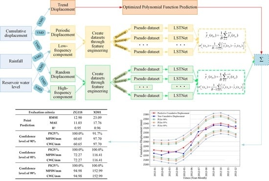
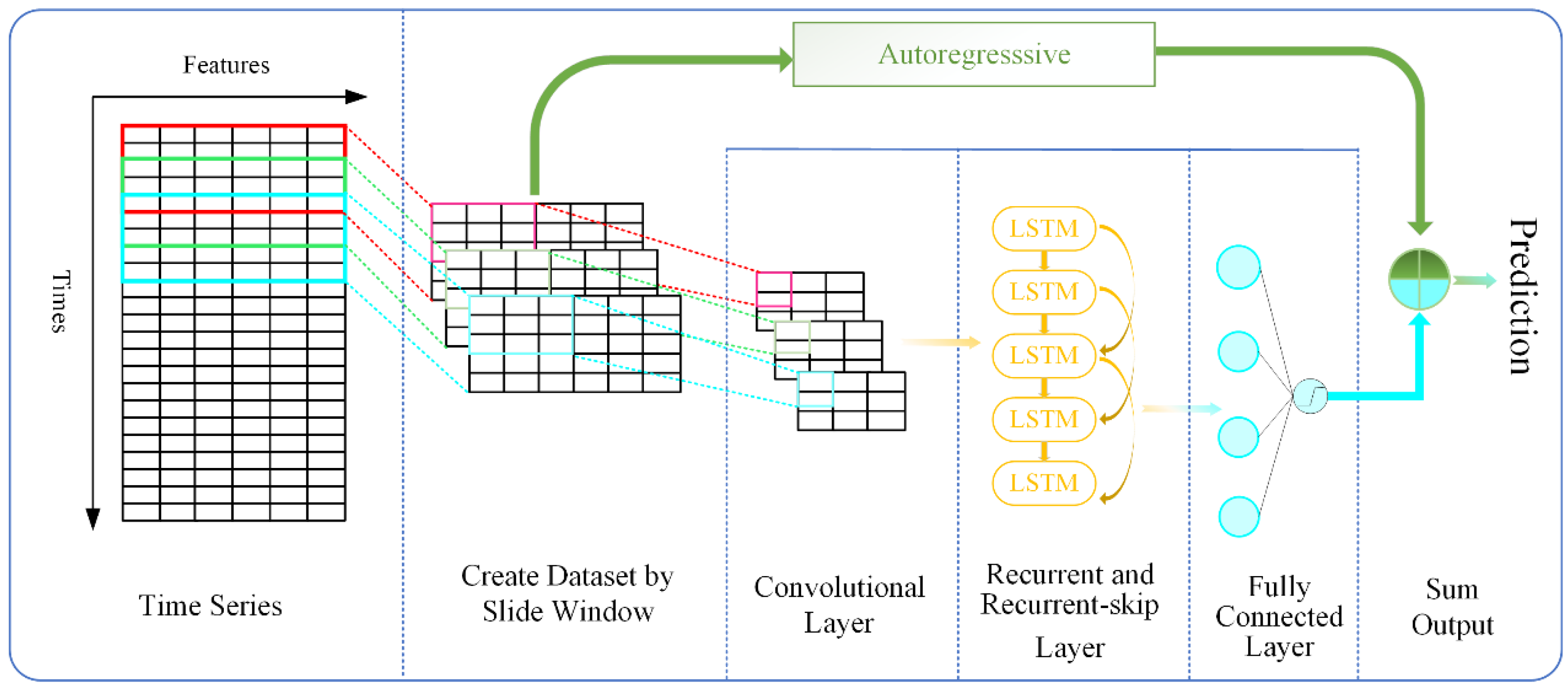


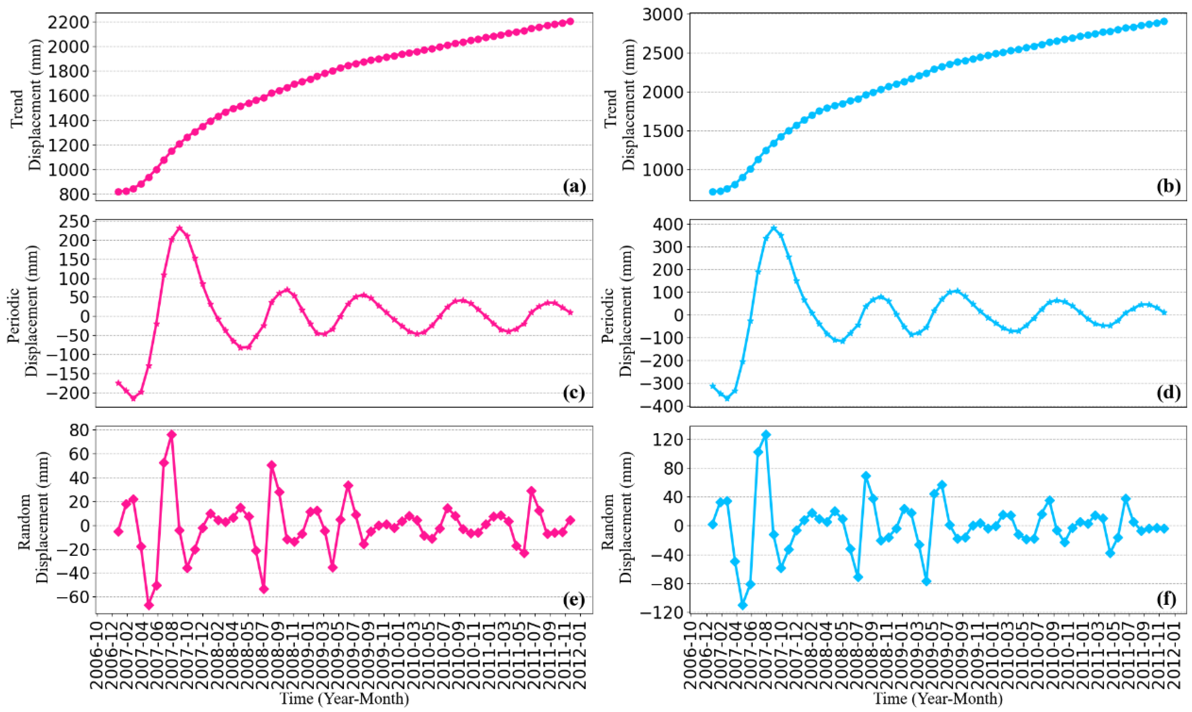

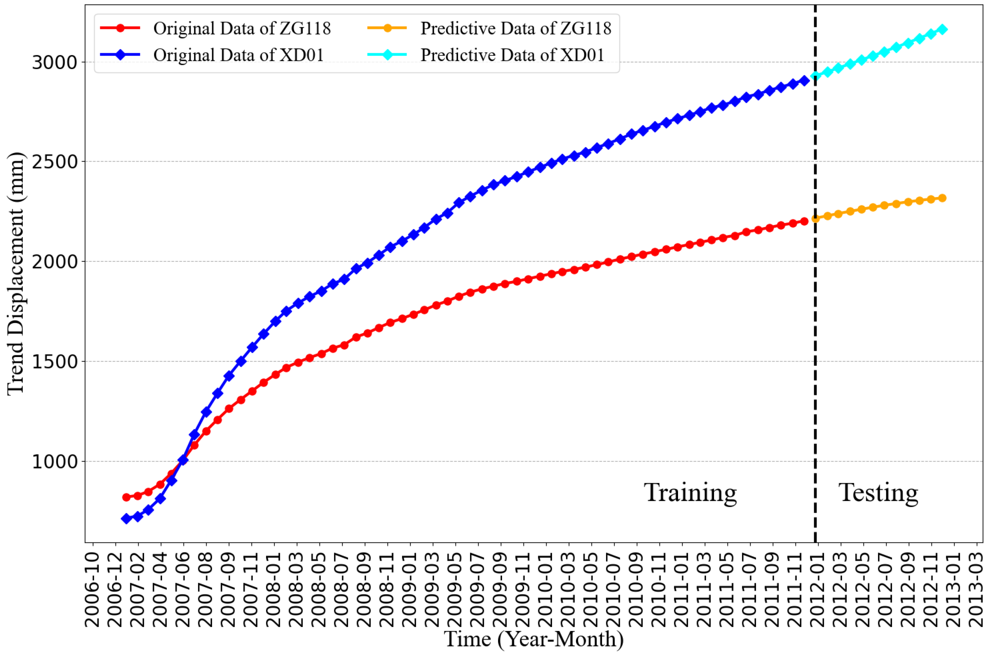

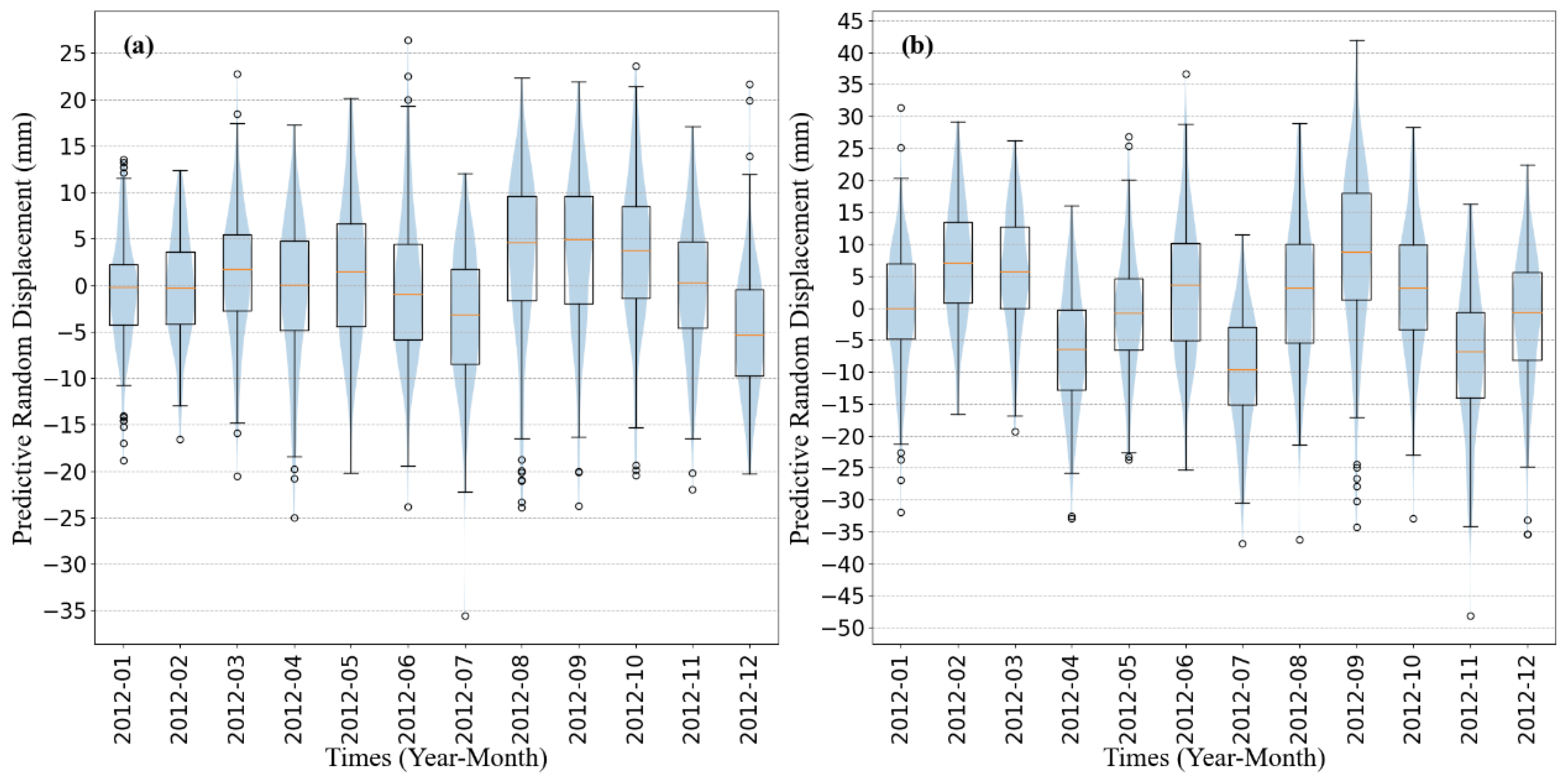


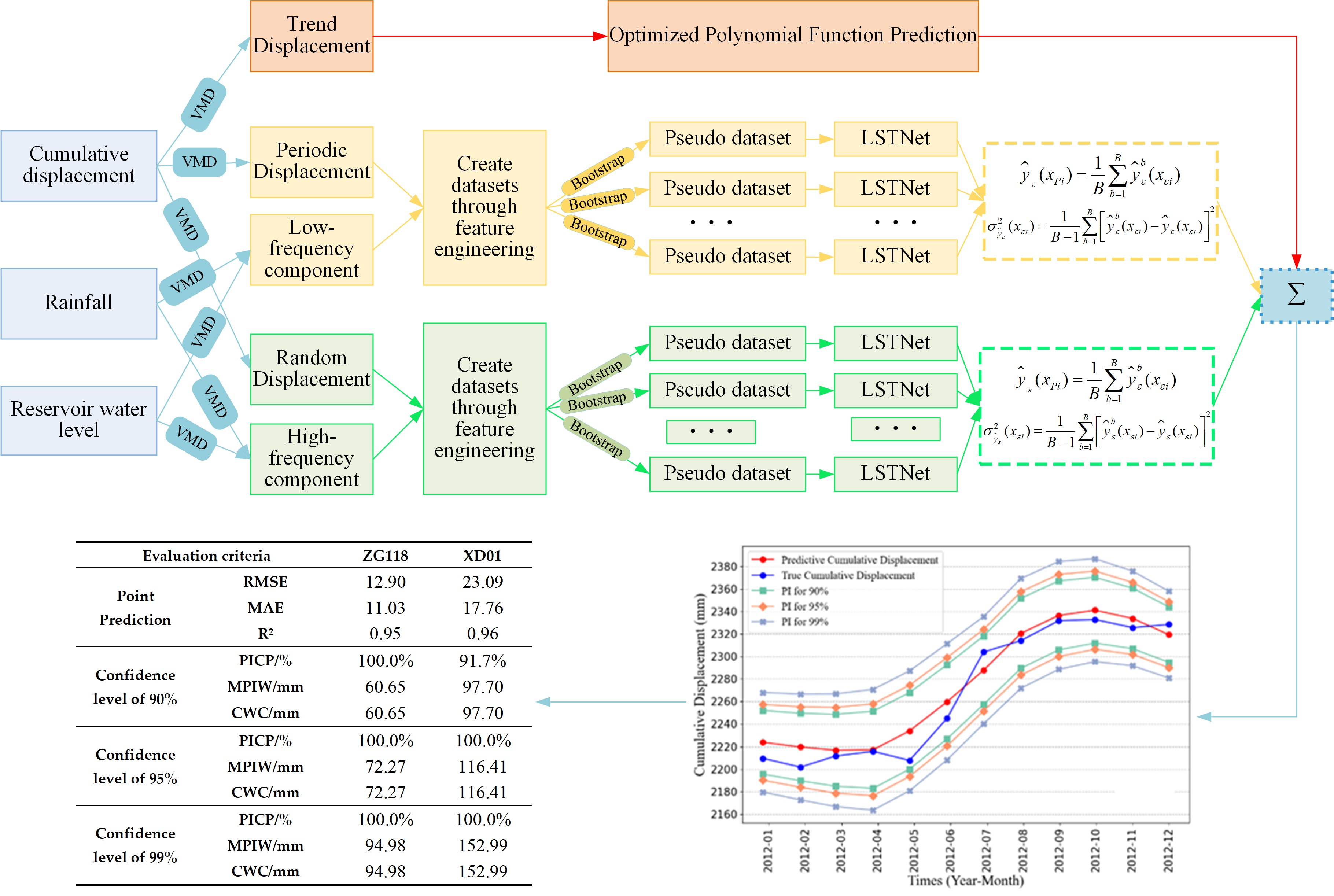
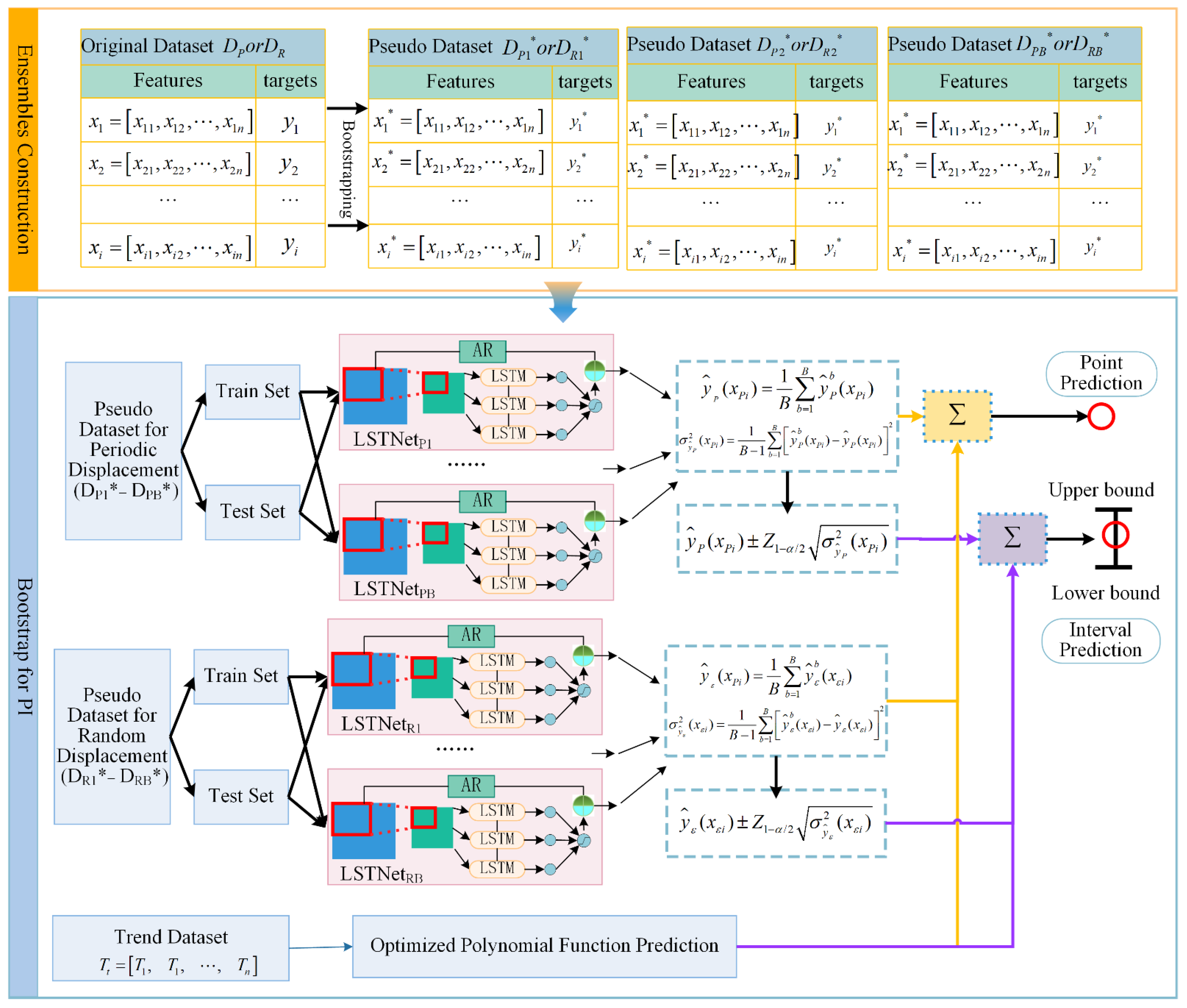
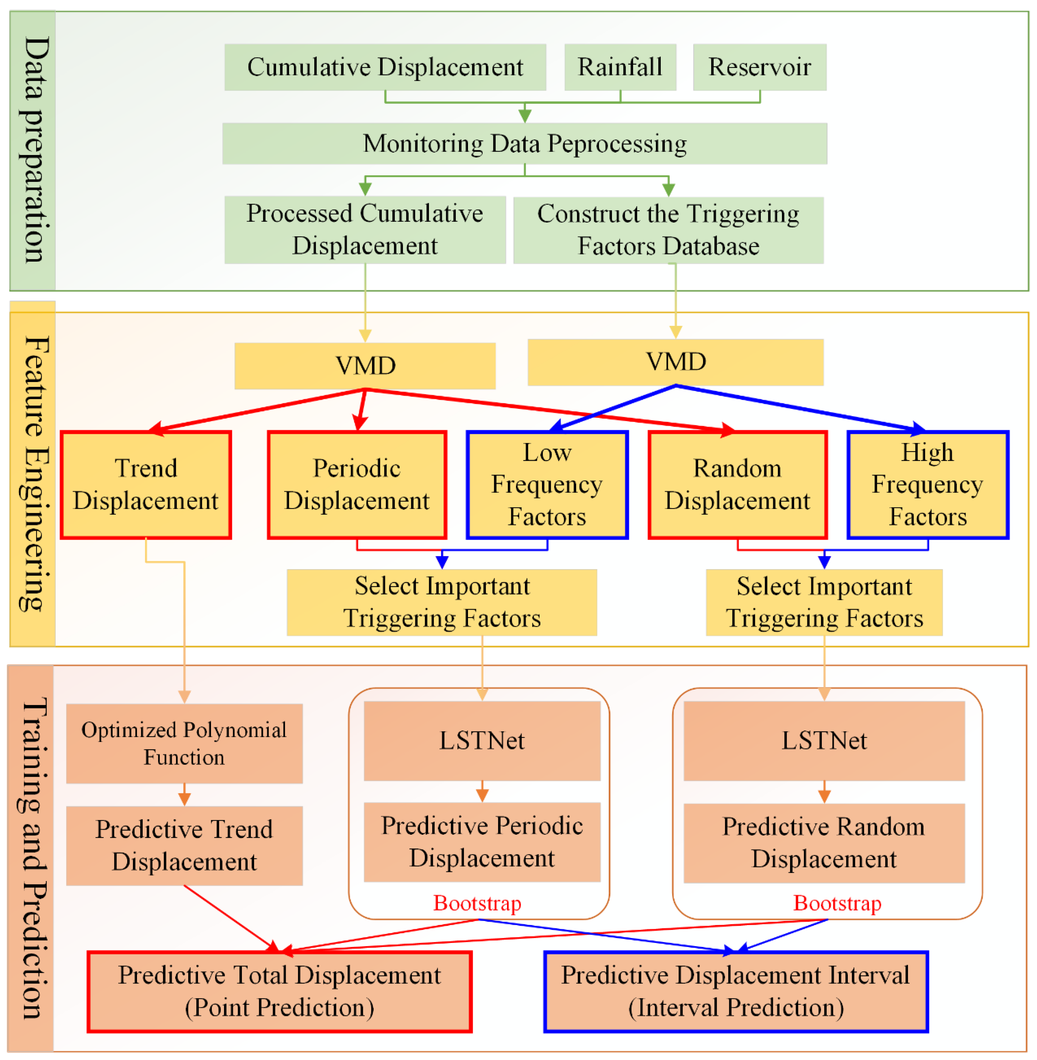
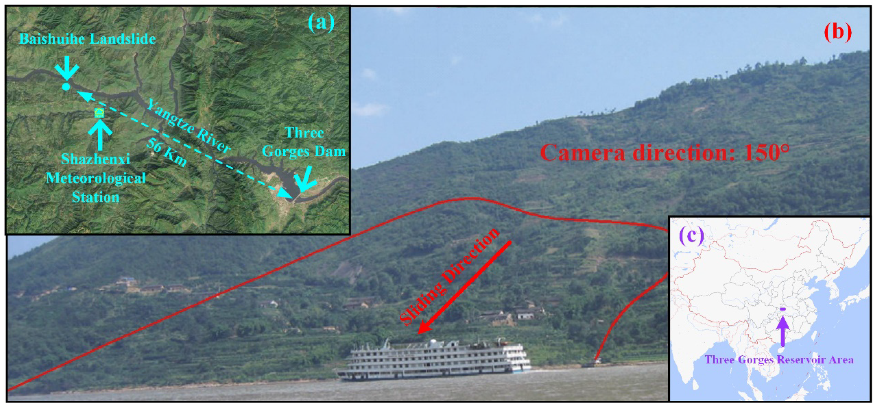
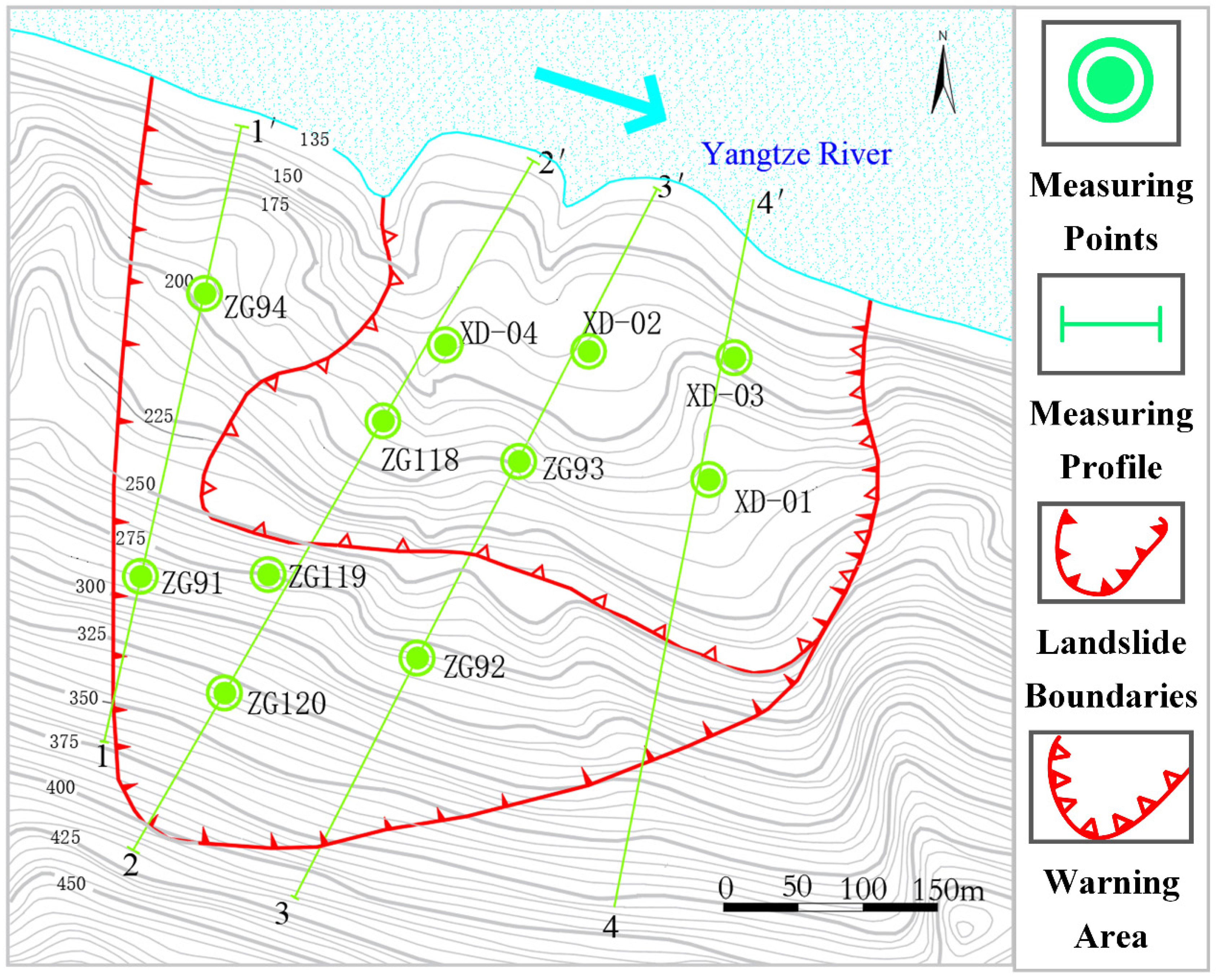
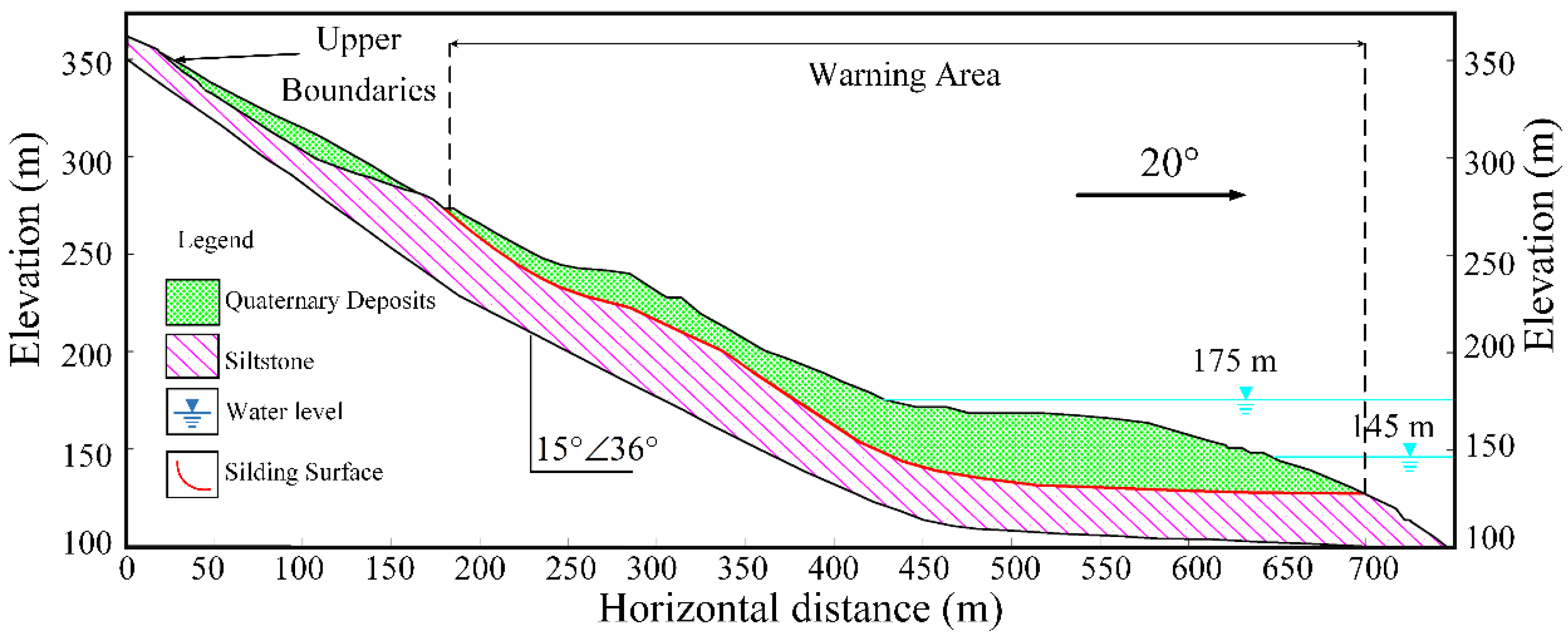
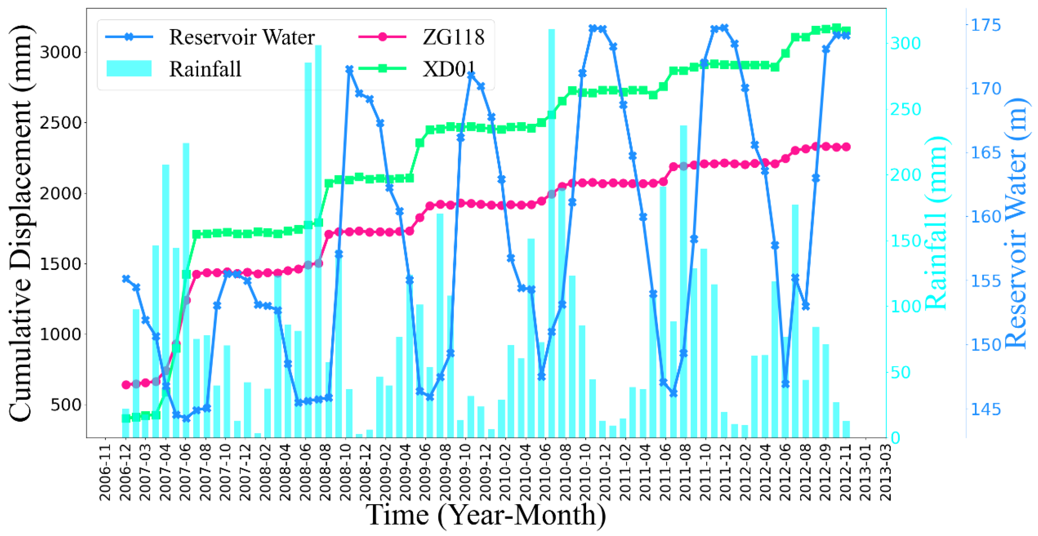
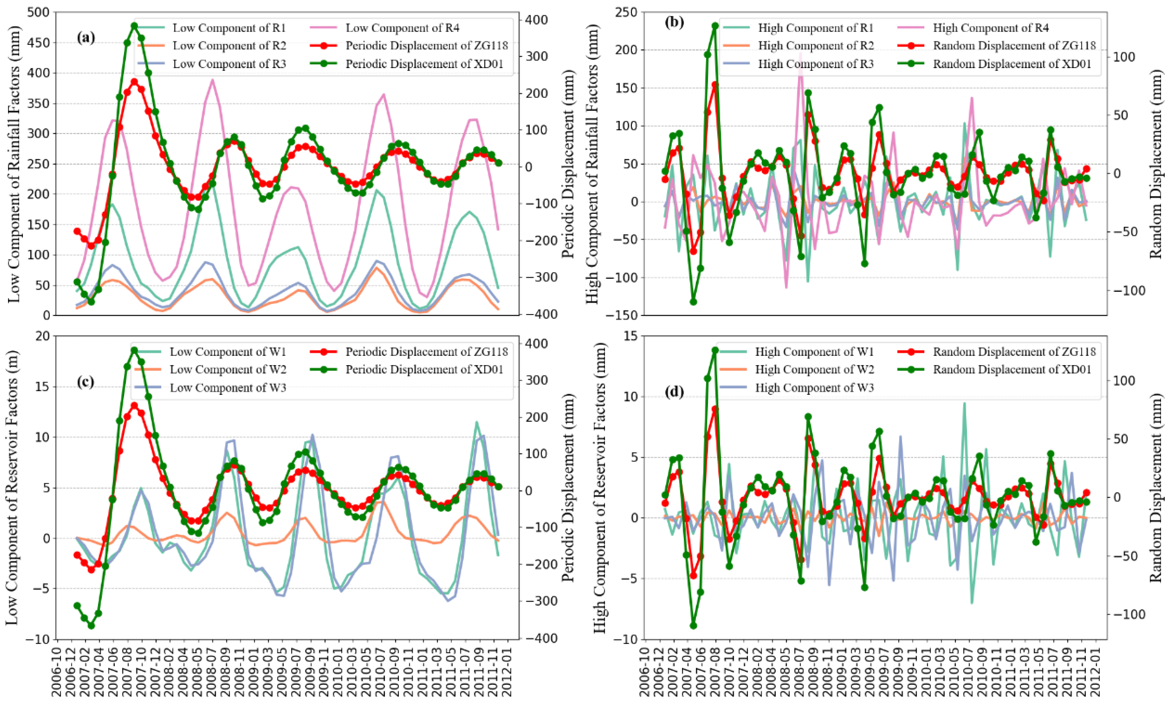
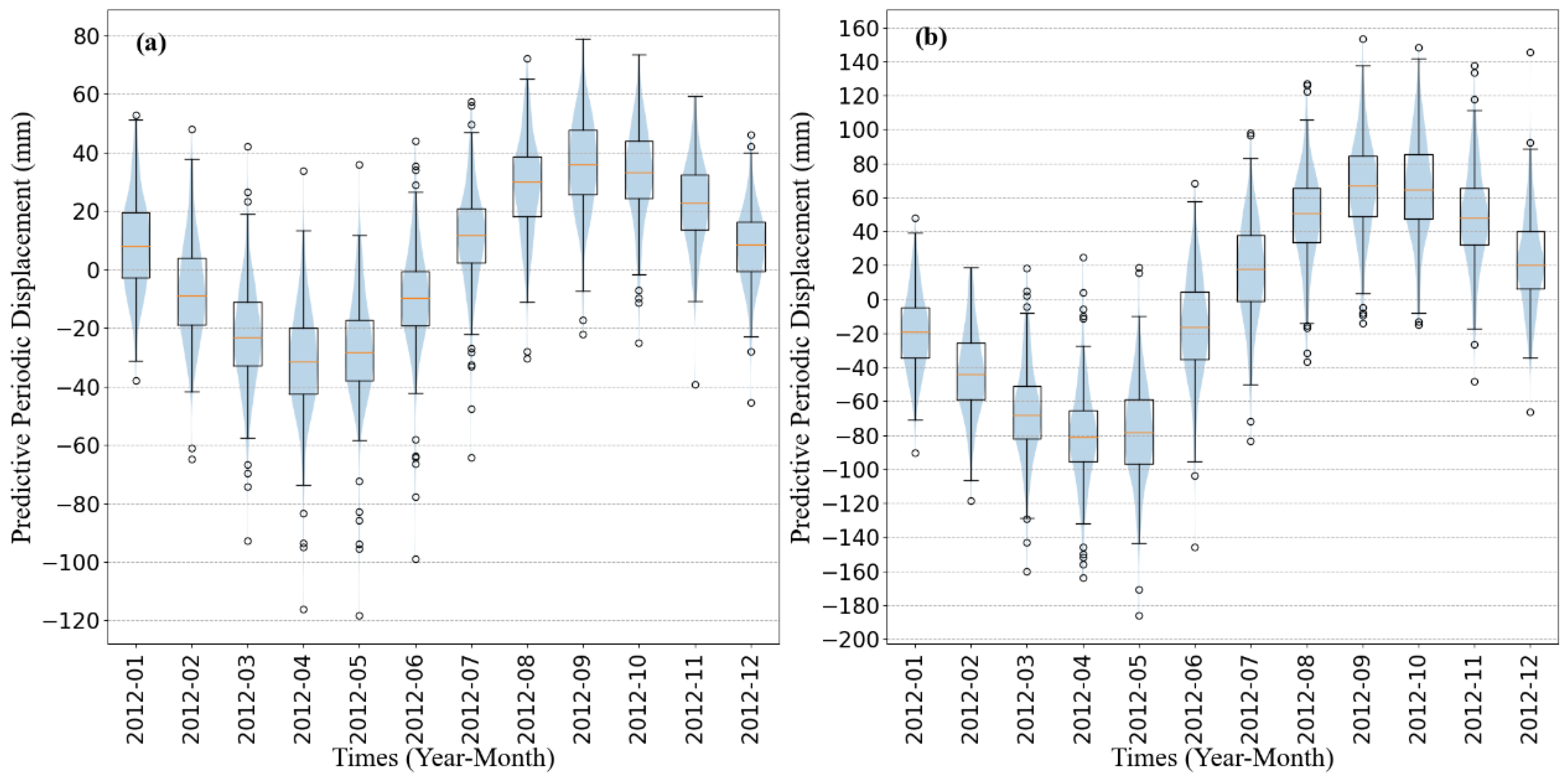
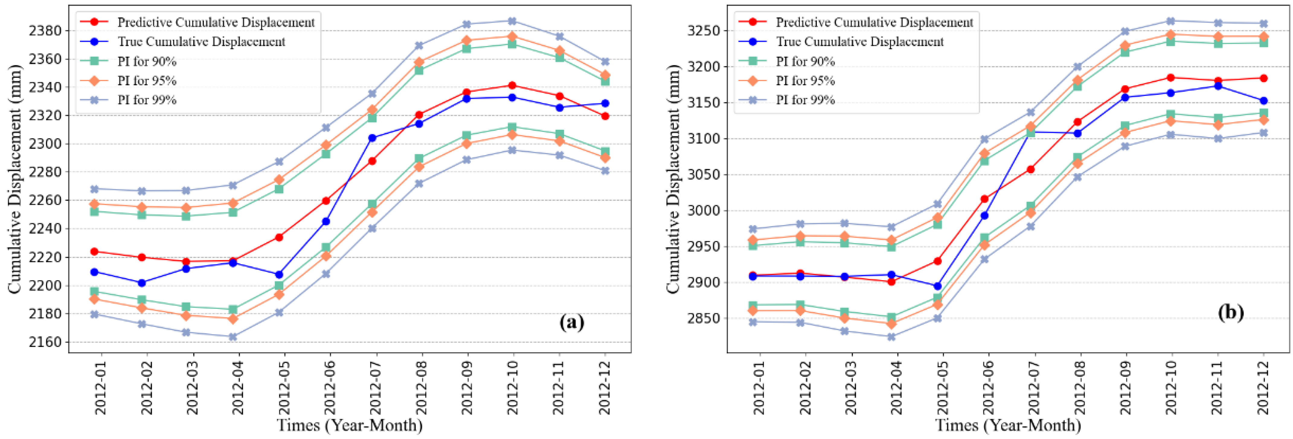
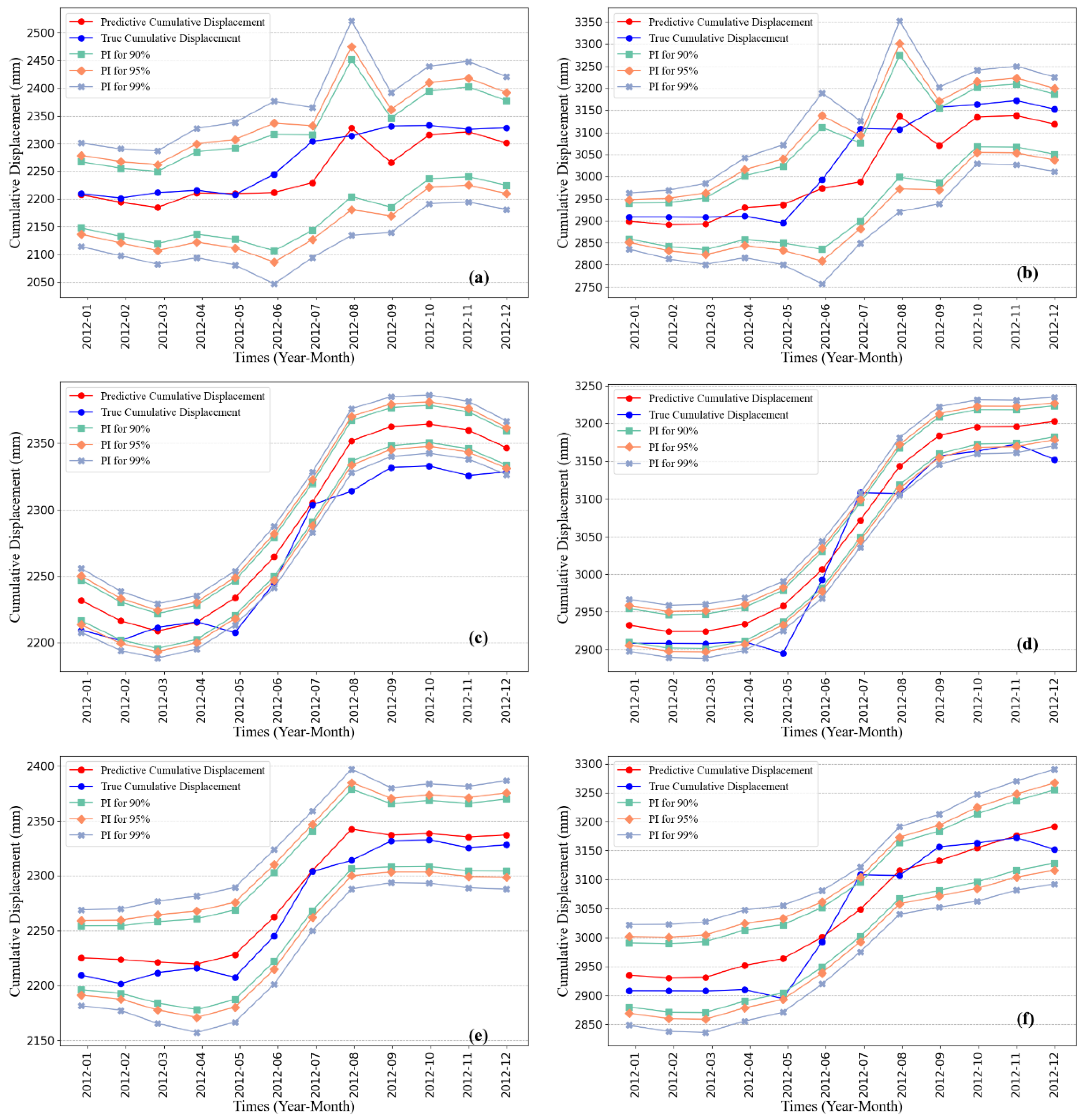