
Monitoring and Integrating the Changes in Vegetated Areas with the Rate of Groundwater Use in Arid Regions †


Abstract

1. Introduction
2. Materials
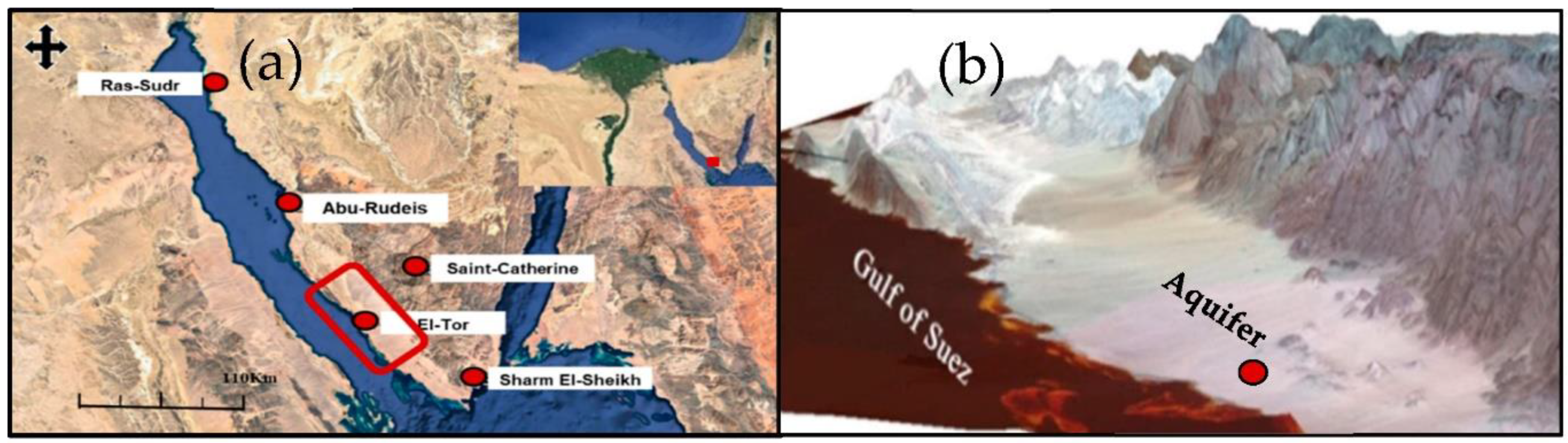
2.1. Study Area
2.2. Landsat 7 & 8
2.3. Sentinel 2A
2.4. Site Measurements
2.5. Software
3. Methods
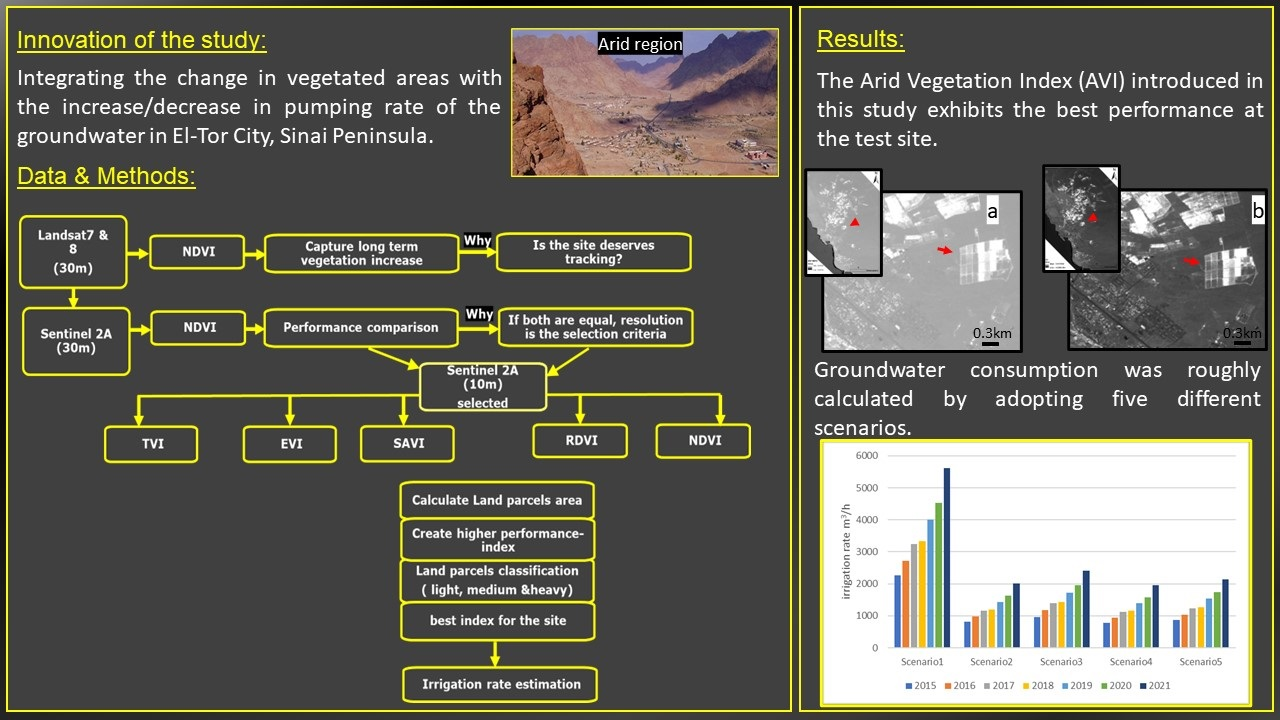
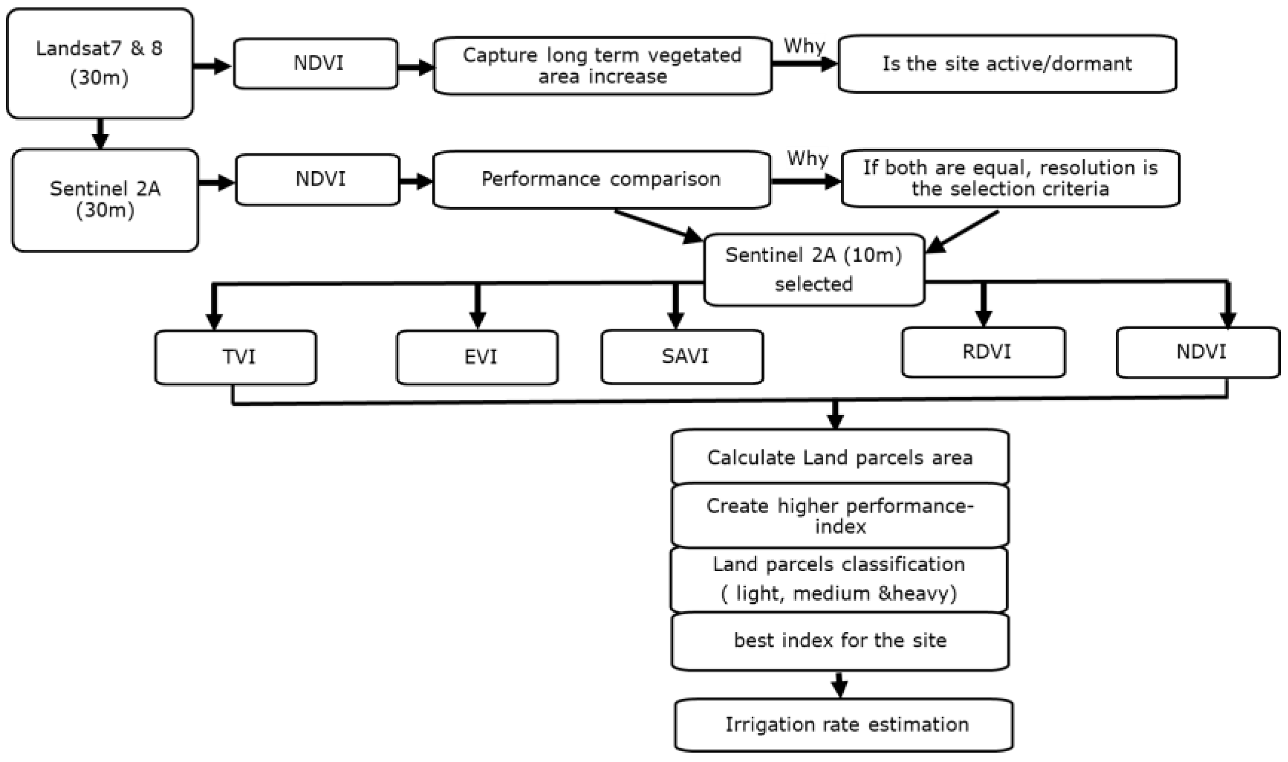
3.1. Tracking the Increase/Decrease in Vegetated Areas
3.2. Testing Different Vegetation Indices
3.3. The Arid Vegetation Index (AVI)
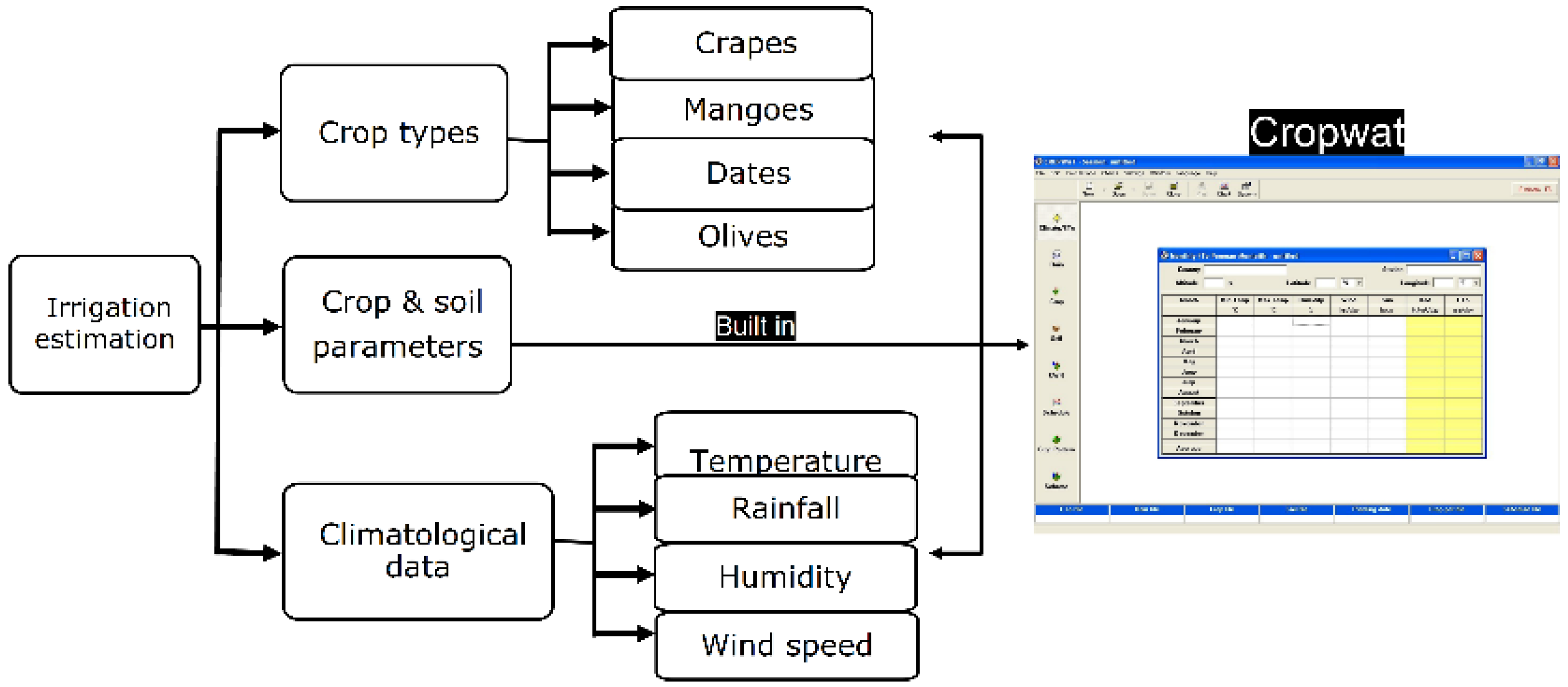
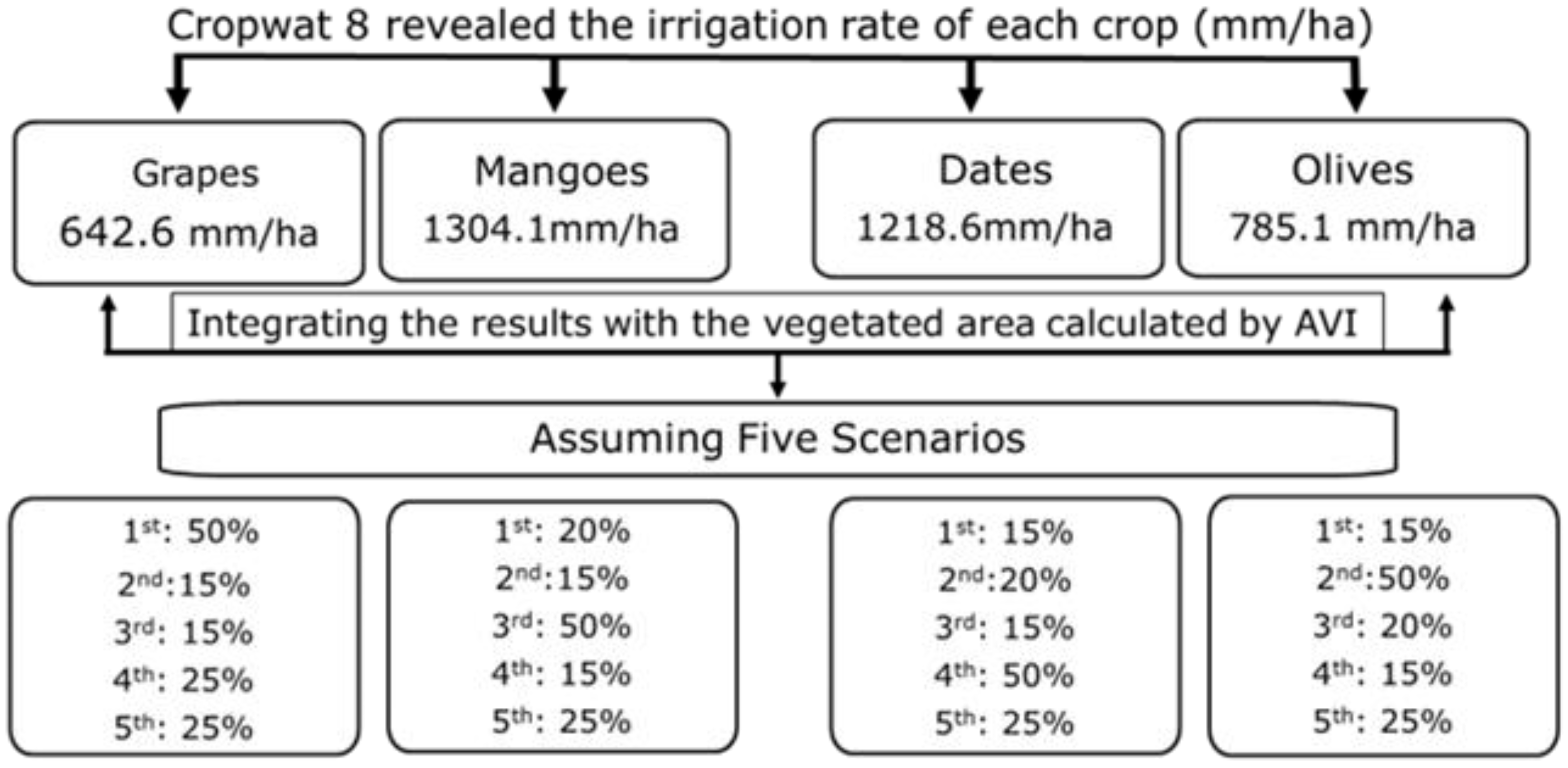
3.4. Crop Consumption Rate Measurements
4. Results
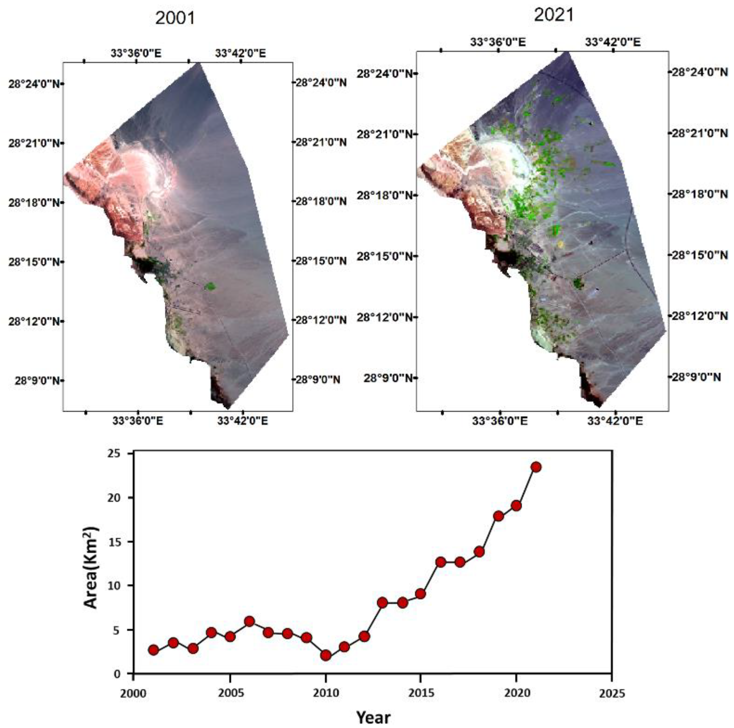
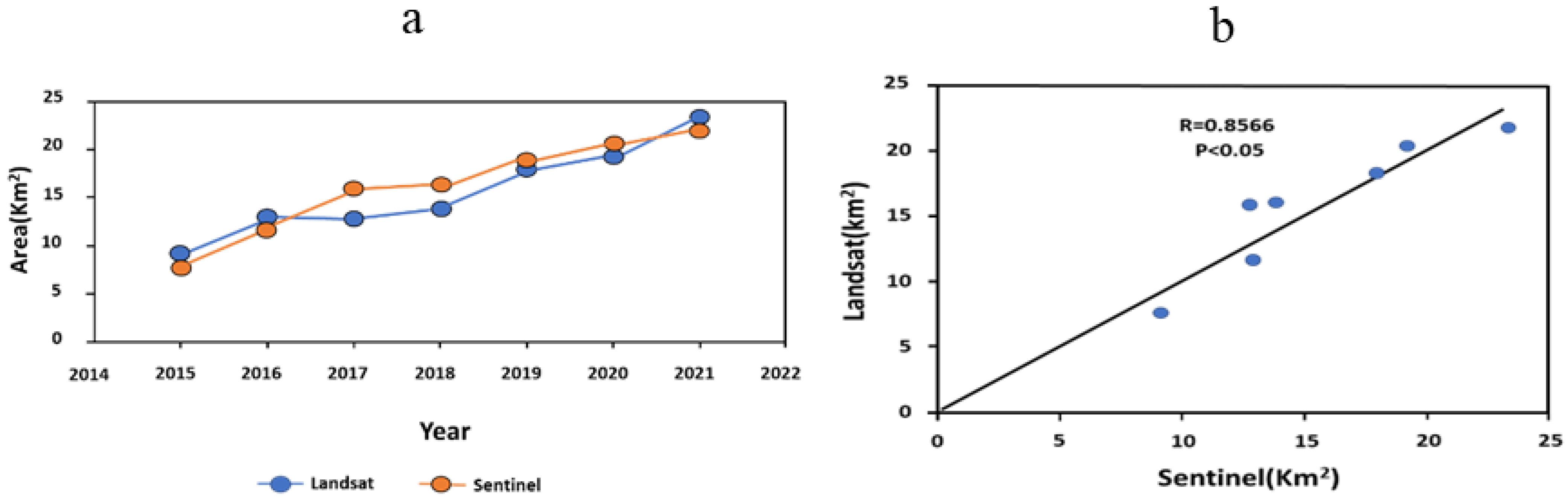
4.1. Tracking Increase/Decrease in Vegetated Areas
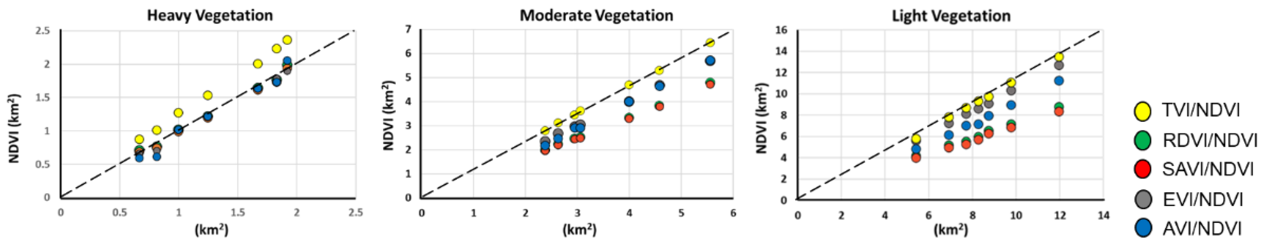
4.2. Testing Different Vegetation Indices
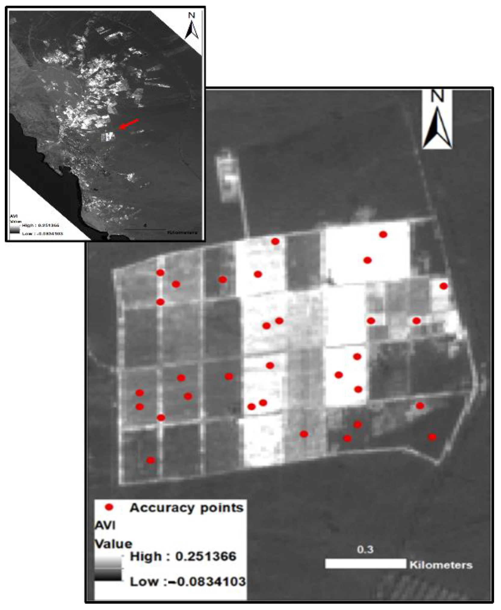
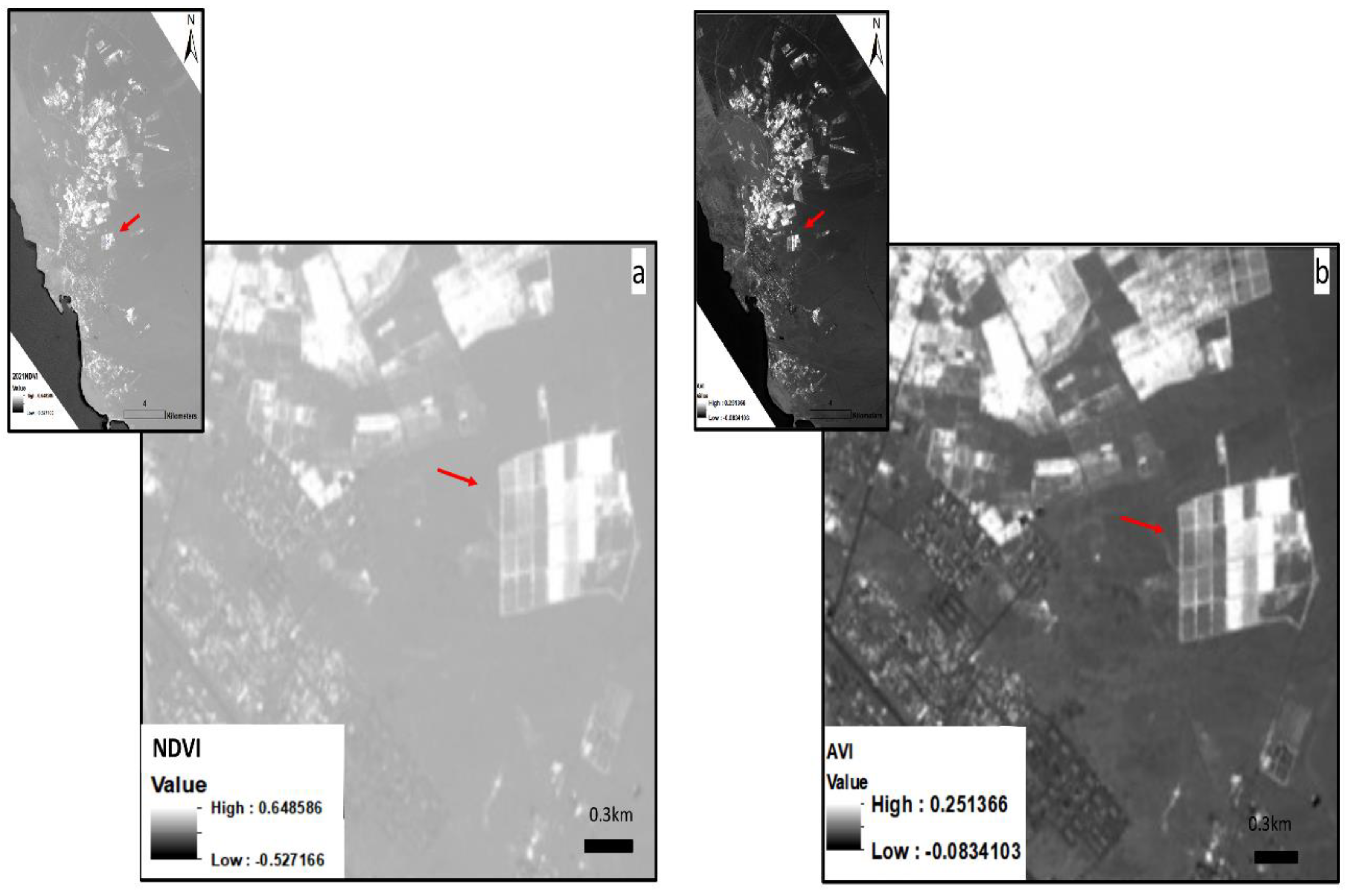
4.3. Testing the Accuracy of AVI
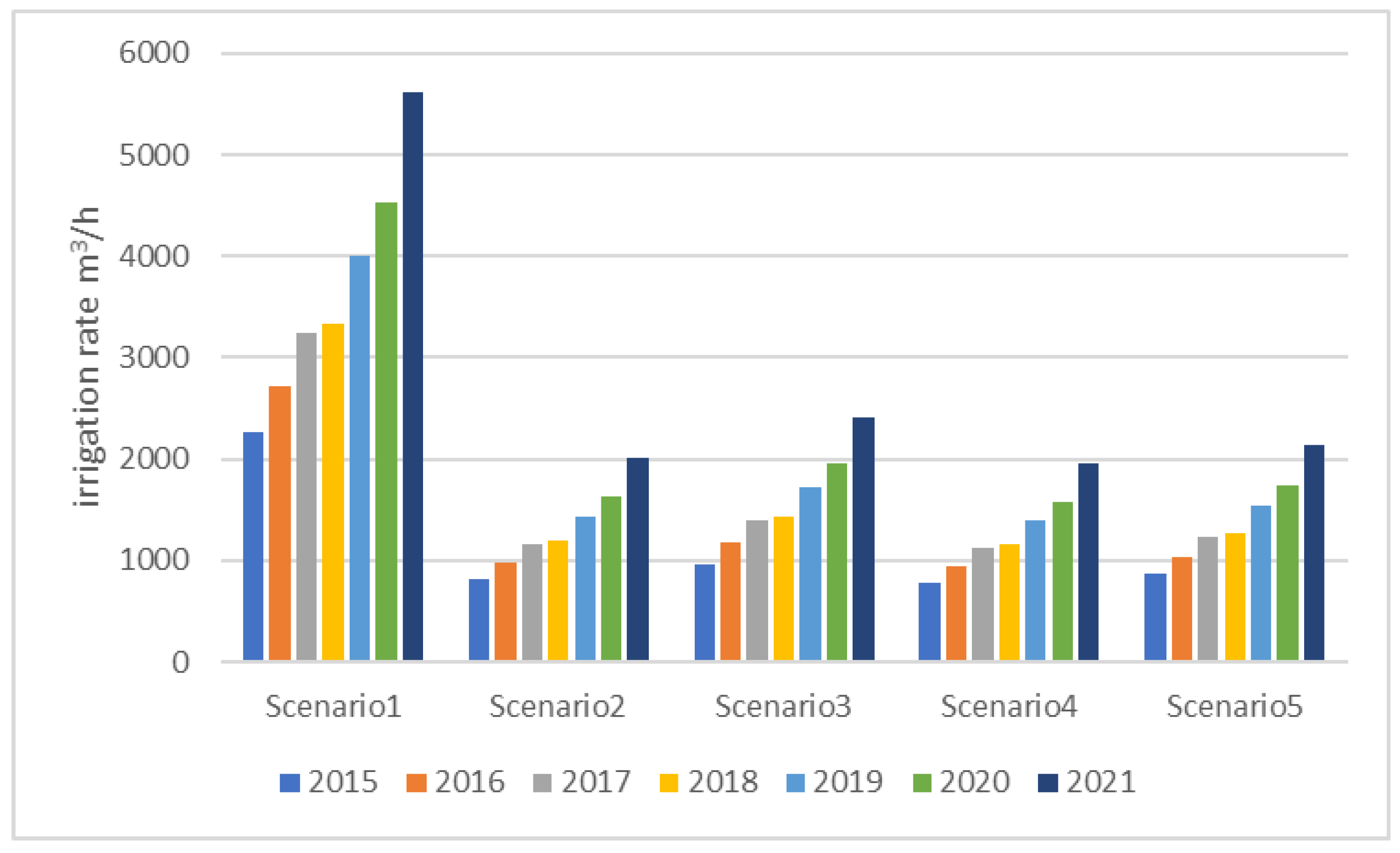
4.4. Crop Consumption Rate Measurements
5. Discussion
6. Concluding Remarks
Author Contributions
Funding
Data Availability Statement
Acknowledgments
Conflicts of Interest
References
- Dregne, H.; Kassas, M.; Rozanov, B. A New Assessment of the World Status of Desertification. Desertif. Control Bull. 1991, 20, 6–29. [Google Scholar]
- Scanlon, B.R.; Keese, K.E.; Flint, A.L.; Flint, L.E.; Gaye, C.B.; Edmunds, W.M.; Simmers, I. Global Synthesis of Groundwater Recharge in Semiarid and Arid Regions. Hydrol. Process. 2006, 20, 3335–3370. [Google Scholar] [CrossRef]
- Yin, L.; Zhang, E.; Wang, X.; Wenninger, J.; Dong, J.; Guo, L.; Huang, J. A GIS-Based DRASTIC Model for Assessing Groundwater Vulnerability in the Ordos Plateau, China. Environ. Earth Sci. 2013, 69, 171–185. [Google Scholar] [CrossRef]
- Morsy, M.; Scholten, T.; Michaelides, S.; Borg, E.; Sherief, Y.; Dietrich, P. Comparative Analysis of TMPA and IMERG Precipitation Datasets in the Arid Environment of El-Qaa Plain, Sinai. Remote Sens. 2021, 13, 588. [Google Scholar] [CrossRef]
- Sheffield, J.; Wood, E.F.; Pan, M.; Beck, H.; Coccia, G.; Serrat-Capdevila, A.; Verbist, K. Satellite Remote Sensing for Water Resources Management: Potential for Supporting Sustainable Development in Data-Poor Regions. Water Resour. Res. 2018, 54, 9724–9758. [Google Scholar] [CrossRef]
- Morsy, M.; Taghizadeh-Mehrjardi, R.; Michaelides, S.; Scholten, T.; Dietrich, P.; Schmidt, K. Optimization of Rain Gauge Networks for Arid Regions Based on Remote Sensing Data. Remote Sens. 2021, 13, 4243. [Google Scholar] [CrossRef]
- Makhamreh, Z.; Hdoush, A.A.A.; Ziadat, F.; Kakish, S. Detection of Seasonal Land Use Pattern and Irrigated Crops in Drylands Using Multi-Temporal Sentinel Images. Environ. Earth Sci. 2022, 81, 120. [Google Scholar] [CrossRef]
- Weber, C.; Puissant, A. Urbanization Pressure and Modeling of Urban Growth: Example of the Tunis Metropolitan Area. Remote Sens. Environ. 2003, 86, 341–352. [Google Scholar] [CrossRef]
- Li, H.; Zheng, L.; Lei, Y.; Li, C.; Liu, Z.; Zhang, S. Estimation of Water Consumption and Crop Water Productivity of Winter Wheat in North China Plain Using Remote Sensing Technology. Agric. Water Manag. 2008, 95, 1271–1278. [Google Scholar] [CrossRef]
- Coppin, P.R.; Bauer, M.E. Digital Change Detection in Forest Ecosystems with Remote Sensing Imagery. Remote Sens. Rev. 1996, 13, 207–234. [Google Scholar] [CrossRef]
- Adhikary, P.P.; Chandrasekharan, H.; Dubey, S.K.; Trivedi, S.M.; Dash, C.J. Electrical Resistivity Tomography for Assessment of Groundwater Salinity in West Delhi, India. Arab. J. Geosci. 2015, 8, 2687–2698. [Google Scholar] [CrossRef]
- Elavarasi, S.A.; Akilandeswari, J.; Sathiyabhama, B. A Survey on Partition Clustering Algorithms. Available online: http://www.ijecbs.com/January2011/N6Jan2011.pdf (accessed on 21 August 2021).
- Sherief, Y. Flash Floods and Their Effects on the Development in El-Qaá Plain Area in South Sinai, Egypt, a Study in Applied Geomorphology Using GIS and Remote Sensing. Available online: https://openscience.ub.uni-mainz.de/handle/20.500.12030/2211 (accessed on 11 November 2022).
- EL-Refai, A.A. Water Resources of Southern Sinai, Egypt; Geomorphological and Hydrogeological Studies; University of Cairo: Giza, Egypt, 1992. [Google Scholar]
- El-Fakharany, M.A. Geophysical and Hydrogeochemical Investigations of the Quaternary Aquifer at the Middle Part of El Qaa-Plain SW Sinai, Egypt. Egypt. J. Geol. 2016, 47, 1003–1022. [Google Scholar]
- Ahmed, M.; Sauck, W.; Sultan, M.; Yan, E.; Soliman, F.; Rashed, M. Geophysical Constraints on the Hydrogeologic and Structural Settings of the Gulf of Suez Rift-Related Basins: Case Study from the El Qaa Plain, Sinai, Egypt. Surv. Geophys. 2014, 35, 415–430. [Google Scholar] [CrossRef]
- Rashed, M.; Sauck, W.; Soliman, F. Gravity, Magnetic, and Geoelectric Survey on EL-Qaa Plain, Southwest Sinai, Egypt. In Proceedings of the 8th Conference Geology of Sinai for Development, Ismailia, Egypt, 3 December 2007; pp. 15–20. [Google Scholar]
- Wahid, A.; Madden, M.; Khalaf, F.; Fathy, I. Geospatial Analysis for the Determination of Hydro-Morphological Characteristics and Assessment of Flash Flood Potentiality in Arid Coastal Plains: A Case in Southwestern Sinai, Egypt. Earth Sci. Res. J. 2016, 20, E1–E9. [Google Scholar] [CrossRef]
- Massoud, U.; Santos, F.; El Qady, G.; Atya, M.; Soliman, M. Identification of the Shallow Subsurface Succession and Investigation of the Seawater Invasion to the Quaternary Aquifer at the Northern Part of El Qaa Plain, Southern Sinai, Egypt by Transient Electromagnetic Data. Geophys. Prospect. 2010, 58, 267–277. [Google Scholar] [CrossRef]
- Goward, S.N.; Masek, J.G.; Williams, D.L.; Irons, J.R.; Thompson, R.J. The Landsat 7 Mission: Terrestrial Research and Applications for the 21st Century. Remote Sens. Environ. 2001, 78, 3–12. [Google Scholar] [CrossRef]
- Irons, J.R.; Dwyer, J.L.; Barsi, J.A. The next Landsat Satellite: The Landsat Data Continuity Mission. Remote Sens. Environ. 2012, 122, 11–21. [Google Scholar] [CrossRef]
- Drusch, M.; Del Bello, U.; Carlier, S.; Colin, O.; Fernandez, V.; Gascon, F.; Hoersch, B.; Isola, C.; Laberinti, P.; Martimort, P.; et al. Sentinel-2: ESA’s Optical High-Resolution Mission for GMES Operational Services. Remote Sens. Environ. 2012, 120, 25–36. [Google Scholar] [CrossRef]
- Gascon, F.; Bouzinac, C.; Thépaut, O.; Jung, M.; Francesconi, B.; Louis, J.; Lonjou, V.; Lafrance, B.; Massera, S.; Gaudel-Vacaresse, A.; et al. Copernicus Sentinel-2A Calibration and Products Validation Status. Remote Sens. 2017, 9, 584. [Google Scholar] [CrossRef]
- Clerici, N.; Valbuena Calderón, C.A.; Posada, J.M. Fusion of Sentinel-1a and Sentinel-2A Data for Land Cover Mapping: A Case Study in the Lower Magdalena Region, Colombia. J. Maps 2017, 13, 718–726. [Google Scholar] [CrossRef]
- Shekhar, S.; Kumar, S.; Sinha, R.; Gupta, S.; Densmore, A.; Rai, S.P.; Kumar, M.; Singh, A.; Van Dijk, W.; Joshi, S.; et al. Efficient Conjunctive Use of Surface and Groundwater Can Prevent Seasonal Death of Non-Glacial Linked Rivers in Groundwater Stressed Areas. In Clean and Sustainable Groundwater in India; Springer: Singapore, 2018; pp. 117–124. [Google Scholar] [CrossRef]
- Jia, K.; Li, Y.; Liang, S.; Wei, X.; Yao, Y. Combining Estimation of Green Vegetation Fraction in an Arid Region from Landsat 7 ETM+ Data. Remote Sens. 2017, 9, 1121. [Google Scholar] [CrossRef]
- Nutini, F.; Boschetti, M.; Brivio, P.A.; Bocchi, S.; Antoninetti, M. Land-Use and Land-Cover Change Detection in a Semi-Arid Area of Niger Using Multi-Temporal Analysis of Landsat Images. Int. J. Remote Sens. 2013, 34, 4769–4790. [Google Scholar] [CrossRef]
- Pettorelli, N.; Vik, J.O.; Mysterud, A.; Gaillard, J.M.; Tucker, C.J.; Stenseth, N.C. Using the Satellite-Derived NDVI to Assess Ecological Responses to Environmental Change. Trends Ecol. Evol. 2005, 20, 503–510. [Google Scholar] [CrossRef] [PubMed]
- Chen, J.M. Evaluation of Vegetation Indices and a Modified Simple Ratio for Boreal Applications. Can. J. Remote Sens. 1996, 22, 229–242. [Google Scholar] [CrossRef]
- Huete, A.R. A Soil-Adjusted Vegetation Index (SAVI). Remote Sens. Environ. 1988, 25, 295–309. [Google Scholar] [CrossRef]
- Huete, A.; Didan, K.; Miura, T.; Rodriguez, E.P.; Gao, X.; Ferreira, L.G. Overview of the Radiometric and Biophysical Performance of the MODIS Vegetation Indices. Remote Sens. Environ. 2002, 83, 195–213. [Google Scholar] [CrossRef]
- Mutanga, O.; Skidmore, A.K. Narrow Band Vegetation Indices Overcome the Saturation Problem in Biomass Estimation. Int. J. Remote Sens. 2004, 25, 3999–4014. [Google Scholar] [CrossRef]
- Tan, M.; Zheng, L. Different Irrigationwater Requirements of Seed Corn and Field Corn in the Heihe River Basin. Water 2017, 9, 606. [Google Scholar] [CrossRef]
- Allen, R.G.; Pruitt, W.O.; Wright, J.L.; Howell, T.A.; Ventura, F.; Snyder, R.; Itenfisu, D.; Steduto, P.; Berengena, J.; Yrisarry, J.B.; et al. A Recommendation on Standardized Surface Resistance for Hourly Calculation of Reference ETo by the FAO56 Penman-Monteith Method. Agric. Water Manag. 2006, 81, 1–22. [Google Scholar] [CrossRef]
- Karnieli, A.; Shachak, M.; Tsoar, H.; Zaady, E.; Kaufman, Y.; Danin, A.; Porter, W. The Effect of Microphytes on the Spectral Reflectance of Vegetation in Semiarid Regions. Remote Sens. Environ. 1996, 57, 88–96. [Google Scholar] [CrossRef]
- Saravanan, K.; Saravanan, R. Determination of Water Requirements of Main Crops in the Tank Irrigation Command Area Using CROPWAT 8.0. Int. J. Interdiscip. Multidiscip. Stud. (IJIMS) 2014, 1, 266–272. [Google Scholar]
- Zhu, Y.; Luo, P.; Zhang, S.; Sun, B. Spatiotemporal Analysis of Hydrological Variations and Their Impacts on Vegetation in Semiarid Areas from Multiple Satellite Data. Remote Sens. 2020, 12, 4177. [Google Scholar] [CrossRef]
- Huang, F.; Zhang, D.; Chen, X. Vegetation Response to Groundwater Variation in Arid Environments: Visualization of Research Evolution, Synthesis of Response Types, and Estimation of Groundwater Threshold. Int. J. Environ. Res. Public Health 2019, 16, 1849. [Google Scholar] [CrossRef]
- Halipu, A.; Wang, X.; Iwasaki, E.; Yang, W.; Kondoh, A. Quantifying Water Consumption through the Satellite Estimation of Land Use/Land Cover and Groundwater Storage Changes in a Hyper-Arid Region of Egypt. Remote Sens. 2022, 14, 2608. [Google Scholar] [CrossRef]
- Wei, S.; Xu, T.; Niu, G.Y.; Zeng, R. Estimating Irrigation Water Consumption Using Machine Learning and Remote Sensing Data in Kansas High Plains. Remote Sens. 2022, 14, 3004. [Google Scholar] [CrossRef]
- Basack, S.; Loganathan, M.K.; Goswami, G.; Khabbaz, H. Saltwater Intrusion into Coastal Aquifers and Associated Risk Management: Critical Review and Research Directives. J. Coast. Res. 2022, 38, 654–672. [Google Scholar] [CrossRef]
- Nigatu, Z.M.; Fan, D.; You, W.; Melesse, A.M.; Pu, L.; Yang, X.; Wan, X.; Jiang, Z. Crop Production Response to Soil Moisture and Groundwater Depletion in the Nile Basin Based on Multi-Source Data. Sci. Total Environ. 2022, 825, 154007. [Google Scholar] [CrossRef]


| Index | NDVI | SAVI | EVI | RDVI | TVI | AVI |
|---|---|---|---|---|---|---|
| Accuracy | 83.3% | 66.6% | 86.6% | 76.6% | 80% | 96.6% |
| EFF (mm) | ETC (mm) | IR (mm) | ||
|---|---|---|---|---|
| Group | Grapes | 7.9 | 655.6 | 642.6 |
| Mangoes | 7.9 | 1322.6 | 1304.1 | |
| Dates | 7.9 | 1237.5 | 1218.6 | |
| Olives | 3.8 | 789 | 785.1 | |
Publisher’s Note: MDPI stays neutral with regard to jurisdictional claims in published maps and institutional affiliations. |
© 2022 by the authors. Licensee MDPI, Basel, Switzerland. This article is an open access article distributed under the terms and conditions of the Creative Commons Attribution (CC BY) license (https://creativecommons.org/licenses/by/4.0/).
Share and Cite
Morsy, M.; Michaelides, S.; Scholten, T.; Dietrich, P. Monitoring and Integrating the Changes in Vegetated Areas with the Rate of Groundwater Use in Arid Regions. Remote Sens. 2022, 14, 5767. https://doi.org/10.3390/rs14225767
Morsy M, Michaelides S, Scholten T, Dietrich P. Monitoring and Integrating the Changes in Vegetated Areas with the Rate of Groundwater Use in Arid Regions. Remote Sensing. 2022; 14(22):5767. https://doi.org/10.3390/rs14225767
Chicago/Turabian StyleMorsy, Mona, Silas Michaelides, Thomas Scholten, and Peter Dietrich. 2022. "Monitoring and Integrating the Changes in Vegetated Areas with the Rate of Groundwater Use in Arid Regions" Remote Sensing 14, no. 22: 5767. https://doi.org/10.3390/rs14225767
APA StyleMorsy, M., Michaelides, S., Scholten, T., & Dietrich, P. (2022). Monitoring and Integrating the Changes in Vegetated Areas with the Rate of Groundwater Use in Arid Regions. Remote Sensing, 14(22), 5767. https://doi.org/10.3390/rs14225767